A two-component jet model for the tidal disruption event Swift J164449.3+573451

Abstract

We analyze both the early and late time radio and X-ray data of the tidal disruption event Swift J1644+57. The data at early times ($\lesssim 5$ days) necessitates separation of the radio and X-ray emission regions, either spatially or in velocity space. This leads us to suggest a two component jet model, in which the inner jet is initially relativistic with Lorentz factor $\Gamma\approx 15$, while the outer jet is trans-relativistic, with $\Gamma\lesssim 1.2$. This model enables a self-consistent interpretation of the late time radio data, both in terms of peak frequency and flux. We solve the dynamics, radiative cooling and expected radiation from both jet components. We show that while during the first month synchrotron emission from the outer jet dominates the radio emission, at later times radiation from ambient gas collected by the inner jet dominates. This provides a natural explanation to the observed re-brightening, without the need for late time inner engine activity. After $100$ days, the radio emission peak is in the optically thick regime, leading to a decay of both the flux and peak frequency at later times. Our model’s predictions for the evolution of radio emission in jetted tidal disruption events can be tested by future observations.

1 Introduction

A stray star, when passing near a massive black hole (MBH) can be torn apart by gravitational forces, leading to a tidal disruption event (TDE). Such an event would be observed as bright emission from a previously dormant MBH, as it is being fed by temporary mass accretion established after the tidal disruption of a passing star (Hills, 1975; Rees, 1988; Evans & Kochanek, 1989). On 28 March 2011, an unusual transient source Swift J164449.3+573451 (hereafter Sw J1644+57) was reported, potentially representing such an event (Burrows et al., 2011; Levan et al., 2011). This event was found to be in positional coincidence ($\lesssim 0.2$ kpc) with a previously dormant host galaxy nucleus, at redshift $z=0.354$ (Levan et al., 2011; Fruchter et al., 2011; Berger et al., 2011).

The rapid variability seen in the X-rays, of $\sim 78$ s (Burrows et al., 2011; Bloom et al., 2011), implies a compact source size $\lesssim 0.15$ AU, which is a few times the Schwarzschild radius of $10^{6}M_{\odot}$ MBH (see also Mïller & Gültekin, 2011). When combined with the very high $\gamma$-ray and X-ray luminosity, $\approx 10^{47}\,{\rm erg\,s^{-1}}$ (Burrows et al., 2011; Bloom et al., 2011), which is 2 - 3 orders of magnitude above the Eddington limit of such a MBH, it was concluded that the X-ray emission must originate from a relativistic jet of Lorentz factor $\Gamma\gtrsim 10$ (Bloom et al., 2011) (see, however, Krolik & Piran, 2011; Ouyed et al., 2011; Quataert & Kasen, 2012; Socrates, 2012, for alternative models).

While early works that investigated the expected signal (optical/UV emission) from such an event were focused on the signal from the accreting material of the stellar debris (Rees, 1988; Loeb & Ulmer, 1997; Ulmer, 1999; Bogdanović et al., 2004; Guillochon et al., 2009; Strubbe & Quataert, 2009), recently, the observational signature from a newly formed jet was considered (Giannios & Metzger, 2011; van Velzen et al., 2011; Wang & Cheng, 2012; Metzger et al., 2012; De Colle et al., 2012; Stone & Loeb, 2012). The basic mechanism suggested in these works is similar to the mechanism that is thought to operate in gamma-ray bursts (GRBs), namely energy dissipation by either internal shock waves (Rees & Meszaros, 1994; Paczynski & Xu, 1994) or by an external (forward) shock wave, accompanied at early stages by a reverse shock wave (Rees & Meszaros, 1992; Meszaros & Rees, 1993; Piran et al., 1993; Sari & Piran, 1995). These shock waves, in turn, are believed to accelerate particles and generate strong magnetic fields, thereby producing synchrotron radiation, accompanied by synchrotron self Compton (SSC) emission at high energies.

Indeed, shortly after its discovery, an extensive radio campaign showed that the X-ray emission is accompanied by bright radio emission (Zauderer et al., 2011), which was interpreted as synchrotron emission from the jetted material, thereby supporting this hypothesis. However, a careful analysis revealed that the radio emitting material propagates at a more modest Lorentz factor, $\Gamma\gtrsim 1$ (Zauderer et al., 2011), and therefore the X-ray and radio emission cannot have similar origin. This had led to the suggestion that the X-rays may originate from internal dissipation (Wang & Cheng, 2012), while the radio may originate from the forward shock that propagates into the surrounding material (Metzger et al., 2012; Cao & Wang, 2012).

Late time radio monitoring, extending up to $\approx 582$ days (Berger et al., 2012; Zauderer et al., 2013), revealed an unexpected behavior: after about $\sim 30$ days (observed time), the radio emission showed re-brightening, which lasted up to $\sim 100$ days, after which the radio flux decayed. This re-brightening was not accompanied by re-brightening in the X-ray flux, and is not expected in the context of the forward shock models. This led Berger et al. (2012) to conclude that the radio re-brightening resulted from late time energy injection (however, for alternative views, see Kumar et al. (2013); Barniol Duran & Piran (2013)). Thus, a comprehensive model that considers the temporal as well as combined radio and X-ray spectral data is still lacking.

Any such model must take into account the fact that the emitting material is mildly relativistic at most. First, the radio emitting material propagates at Lorentz factor $\Gamma\gtrsim 1$. Second, while the X-ray emitting material propagates at initial Lorentz factor $\Gamma\simeq 10-20$, its velocity becomes trans-relativistic on the relevant time scale of tens of days, as surrounding material is collected. The dynamics of such trans-relativistic propagation was recently considered by Pe’er (2012).

Here, we propose a new model that considers simultaneously the emission of both the radio and the X-rays, their spectrum as well as temporal evolution. We re-derive the constraints set by both radio and X-ray observations, and confirm that indeed at early times (first few days) these must have a separate origin. We calculate the dynamics of the X-ray emitting plasma as it collects material from the surrounding and decelerates. We show that after $\sim 30$ days (observed time), synchrotron emission from this plasma peaks at radio frequencies, thereby providing a natural explanation to the re-brightening seen at radio frequencies at these times, without the need for late time internal engine activity. Moreover, we show that the decay of the radio flux after $\sim 100$ days is naturally explained by synchrotron self absorption. At this stage, the flow is in the trans-relativistic regime ($\Gamma-1\simeq 1$).

This paper is organized as follows. In §2, we carefully revise the observed data of both the radio and X-ray emission at early times (up to five days). While our treatment is more general than previous works, we confirm earlier conclusions that indeed the radio and X-ray emission must have separate origins. In §3 we consider the temporal evolution of the X-ray emitting material as it slows and cools, and show that it can be the source of the re-brightening at radio frequencies seen after $\sim 30$ days. We further consider radiative cooling in §3.2. We show that the very late ($\gtrsim 100$ days) decay of the radio flux is naturally attributed to emission in the optically thick regime: as the electrons cool, eventually the peak of the synchrotron becomes obscured. We compare our model to the late time radio data of Sw J1644+57 using two scenarios: spherical expansion and lateral expansion in §4, before summarizing our main results in §5.

2 Early time radio and X-ray emission and its interpretation

Sw J1644+57 is a long-lived (duration $\gtrsim$ months) X-ray outburst source, accompanied by bright radio emission, interpreted as synchrotron radiation. During the first few days of observations, the isotropic X-ray luminosity ranged from $\sim 3\times 10^{45}\,{\rm erg\,s^{-1}}$ to a peak as high as $\sim 3\times 10^{48}\,{\rm erg\,s^{-1}}$ (Burrows et al., 2011) with average X-ray luminosity $\approx few\times 10^{47}\,{\rm erg\,s^{-1}}$. The X-ray emission peaked at frequency $\sim 2\times 10^{18}$ Hz, with estimated uncertainty up to two orders of magnitude above this value (Zauderer et al., 2011). During the first few days, the X-ray lightcurve was complex and highly variable, with variability time scale as short as $\sim 100$ s (Burrows et al., 2011; Levan et al., 2011). On the high frequency side ($\sim$ GeV emission), the Fermi LAT upper limits are two orders of magnitude below the X-ray luminosity (Burrows et al., 2011).

This source triggered a radio campaign, that began a few days after its initial discovery. Radio observations showed that the peak frequency occurs at $\sim 8\times 10^{11}\eta$ Hz with uncertainty $1\leq\eta\leq 10$, and peak luminosity $\nu L_{\nu}\gtrsim 10^{43.5}\,{\rm erg\,s^{-1}}$ during the first few days. The spectral energy distribution (SED) at the radio band ($<345$ GHz$)$ at $\Delta t^{\rm ob}\approx 5$ days is well described by a power law, $F_{\nu}\propto\nu^{1.3}$ up to $F_{\nu}(|_{\nu=345{\rm GHz}})\approx 35$ mJy. The steep power law index requires self-absorbed synchrotron emission, with self absorption frequency $\nu_{a}\gtrsim 10^{11}$ Hz (Zauderer et al., 2011; Berger et al., 2012). Within two weeks, the X-rays maintained a more steady level, albeit with episodic brightening and fading spanning more than an order of magnitude in flux, while the low frequency (radio) emission decreased markedly in this period (Levan et al., 2011; Zauderer et al., 2011).

In this section, we interpret the publicly available radio and X-ray data at 5 days in the framework of the synchrotron (radio) and the inverse Compton (X-rays) model. As we show below, in spite of the relatively large number of free model parameters, the constraints set by the existing early time data exclude this model: the same electrons cannot be responsible for simultaneous emission of both the radio and X-ray photons in the framework of this model. We provide in table 1 below constraints on (some of the) free model parameters derived from existing data, and show that either of the three: the emission radius (corresponding to observed time of 5 days), the bulk motion Lorentz factor or the emitting electrons characteristic Lorentz factor cannot be the same for the two (radio and X-rays) emitting regions. This leads us to suggest an alternative model, that of the structured jet, to be discussed below.

2.1 Interpretation of early radio emission

The radio emission observed from Swift J1644+57 is assumed to have synchrotron origin. The synchrotron emitting plasma can be described by five free parameters: the source size $R$, bulk Lorentz factor $\Gamma$, total number of radiating electrons $N_{\rm e}$, magnetic field strength $B$, and the characteristic electron Lorentz factor (as is measured in the plasma frame), $\gamma_{e}$. Calculations of the values of these parameters appear in Zauderer et al. (2011). Here, we generalize the treatment in Zauderer et al. (2011) by removing the equipartition assumption used in that work.

Existing data provides the following four constraints. The observed characteristic frequency and total luminosity of synchrotron emission, $\nu_{m}^{\rm ob}$ and $\nu L_{\nu}$ are given by (Rybicki & Lightman, 1979)

$$\begin{array}[]{lcl}\nu_{m}^{\rm ob}&=&\frac{3}{4\pi}\frac{q_{e}B}{m_{\rm e}c}\gamma_{e}^{2}\Gamma=4.20\times 10^{6}\;B\,\gamma_{e}^{2}\,\Gamma=8\times 10^{11}~{}{\rm Hz};\\ \nu L_{\nu}&\approx&N_{e}P_{\rm syn}=\frac{4}{3}N_{e}\sigma_{T}c\gamma_{e}^{2}U_{B}\Gamma^{2}=1.06\times 10^{-15}\;N_{e}\,\gamma_{e}^{2}\,B^{2}\,\Gamma^{2}=3\times 10^{43}~{}{\rm erg~{}s^{-1}}.\end{array}$$ (1)

Here and below, $P_{\rm syn}$ is the total synchrotron radiation power, $\sigma_{T}$ is the Thomson cross section, $U_{B}\equiv B^{2}/8\pi$ is the magnetic energy density and CGS units are used. In deriving equation (1), spherical explosion was assumed.

A third condition is the synchrotron self absorption frequency, $\nu_{a}\approx 2\times 10^{11}$ Hz. For $\nu_{a}<\nu_{m}$, as is the case here, the self absorption coefficient scales as $\alpha_{\nu}\propto\nu^{-5/3}$ (see Rybicki & Lightman, 1979, equation (6.50)), thus $\tau_{\nu}/\tau_{\nu_{m}}=\alpha_{\nu}/\alpha_{\nu_{m}}=\left(\nu/\nu_{m}\right)^{-5/3}$. Here, $\tau_{\nu}\propto\alpha_{\nu}$ is the optical depth, $\tau_{\nu_{m}}\equiv\tau_{\nu}(\nu=\nu_{m})=\alpha_{\nu_{m}}R^{\prime}$, and $R^{\prime}=R/\Gamma$ is the co-moving size of the synchrotron emitting region. In calculating $\alpha_{\nu_{m}}$ we use equation (6.53) in Rybicki & Lightman (1979), which assumes power law distribution of electrons above $\gamma_{e}$. We use power law index $p=2$, although the result is found not to be sensitive to neither the power law distribution assumption or the power law index; a similar result is obtained if the electrons assume a thermal distribution. Since, by definition, $\tau_{\nu_{a}}\equiv\tau_{\nu}(\nu=\nu_{a})=1$, the synchrotron self absorption frequency $\nu_{a}$ is

$$\frac{\nu_{a}^{\rm ob}}{\nu_{m}^{ob}}=2.46\times 10^{-6}N_{e}^{3/5}R^{-6/5}B^{-3/5}\gamma_{e}^{-3}\simeq{1\over 4}~{}.$$ (2)

Here, the observed value of the self absorption frequency $\nu_{a}^{\rm ob}\approx 2\times 10^{11}$ Hz is used.

As a fourth condition we use the assumption of ballistic expansion of the source, similar to Zauderer et al. (2011). We consider constant bulk expansion velocity of the source $\beta=\left(1-\Gamma^{-2}\right)^{1/2}$ and head-on emission. At redshift $z=0.354$, an observed time $\Delta t^{\rm ob}=5$ days corresponds to source frame time $\Delta t^{\rm ob}/(1+z)=3.7$ days. Due to relativistic time compression, the actual time that the source would have expanded is $[\Delta t^{\rm ob}/(1+z)]/(1-\beta)$. Thus, the emission radius is related to the observed time by

$$R=\frac{\Delta t^{\rm ob}}{(1+z)}\cdot\frac{\beta c}{(1-\beta)}$$ (3)

The four constraints derived in equations (1) – (3) are insufficient to fully determine the values of the five free model parameters. We therefore choose the source size $R$ at $\Delta t^{\rm ob}=5$ days as a free variable, and determine the values of the other four free parameters. The results of our calculation are shown in Figure 1. We present the bulk Lorentz factor $\Gamma$ (black), bulk momentum $\Gamma\beta$ (cyan), magnetic field $B$ (green), characteristic electron Lorentz factor $\gamma_{e}$ (red) and the number density of the radiating particles, in the observer’s frame, $n_{e}$ (blue).

Figure 1: Dependence of the free model parameters: the bulk Lorentz factor, $\Gamma$ (black), the bulk momentum, $\Gamma\beta$ (cyan), the magnetic field, $B$ (green), the typical Lorentz factor of electrons, $\gamma_{e}$ (red) and the number density of electrons $n_{e}$ (in the observer’s frame) (blue) on the emission radius of the radio photons, $R$, under the assumption that the radio photons originating from synchrotron emission.

In order to constrain the allowed parameter space region, we use two additional assumptions: (1) In Fermi-type acceleration, the typical Lorentz factor of the energetic electrons $\gamma_{e}\leq m_{p}/m_{e}=1836$ in the rest frame of the plasma. This assumption follows an equipartition assumption between the energy given to the accelerated electrons and protons; (2) As the emission radius is large, the magnetic field must be produced at the shock front. Thus, the ratio of magnetic energy density, $B^{2}/8\pi$ to the photon energy density, $L/(4\pi R^{2}\Gamma^{2}c)$ (often denoted by $\epsilon_{B}$), is smaller than unity. These constraints which are commonly used in modeling, e.g., emission from GRBs, are shown by the dashed lines in Figure 1.

After adding these two constraints, we conclude that the radio emission zone at early times fulfills the following conditions: (i) The emission radius is in the range $3.0\times 10^{15}~{}{\rm cm}\lesssim R\lesssim 1.0\times 10^{16}$ cm. (ii) The outflow is trans-relativistic, with $1.04\lesssim\Gamma\lesssim 1.2$, and $0.24\lesssim\beta\lesssim 0.55$. (iii) The magnetic field is poorly constrained by the data, and could range from $5.0\times 10^{-2}$ G to $7.0$ G. (iv) The electrons are hot, with minimum random Lorentz factor exceeding $\gamma_{e}\gtrsim 150$. (v) The emitting region is dense: $3.0\times 10^{3}~{}{\rm cm}^{-3}<n_{e}<3.0\times 10^{7}~{}{\rm cm}^{-3}$. This result likely excludes shocked external ISM material as the source of the radio emission, as the typical densities of the ISM, $\approx 1-10~{}{\rm cm}^{-3}$ (Baganoff et al., 2003), even after compressed by mild-relativistic shock waves - are much lower than these values. (vi) The total number of radiating particles is at the range $1.0\times 10^{52}<N_{e}<3.4\times 10^{54}$, with likely value of $\sim 10^{53}$. These results are consistent with the results derived by Zauderer et al. (2011).

2.2 Interpretation of early X-ray emission

Our underlying assumption is that the origin of the X-ray emission at early times is mainly due to inverse Compton (IC) scattering of the synchrotron radio photons by relativistic electrons. As we show here, these electrons must be located in a different region than the radio-emitting electrons. Following the treatment by Pe’er & Loeb (2012), two constraints can be put by the data: (I) the ratio of the IC and synchrotron peak frequencies is given by

$$\frac{\nu_{\rm peak,IC}^{\rm ob}}{\nu_{\rm peak,syn}^{\rm ob}}=\frac{4}{3}\left(\gamma_{\rm e[IC]}\Gamma\right)^{2}\simeq{2\times 10^{18}\over 8\times 10^{11}},$$ (4)

and, (II) the ratio of IC to synchrotron peak fluxes is

$$\frac{F_{\nu,\rm IC}}{F_{\nu,\rm syn}}={(\nu F_{\nu,peak,IC}/\nu_{\rm peak,IC})\over(\nu F_{\nu,peak,syn}/\nu_{\rm peak,syn})}=n_{e[IC]}r\sigma_{\rm T}\simeq 4\times 10^{-3}.$$ (5)

Here, $\gamma_{e[IC]}$ and $n_{e[IC]}$ are the typical Lorentz factor and number density of electrons (in the observer’s frame) that emit the IC photons, and $r$ and $\Gamma$ are the typical size and the bulk Lorentz factor of the IC emission region. In estimating the ratio of the peak frequencies and fluxes, we used $\nu_{\rm peak,IC}^{\rm ob}\simeq 2\times 10^{18}$ Hz, $\nu_{\rm peak,syn}^{\rm ob}\simeq 8\times 10^{11}$ Hz, $\nu F_{\nu,peak,IC}\approx 3\times 10^{47}~{}{\rm erg~{}s^{-1}}$, and $\nu F_{\nu,peak,syn}\approx 3\times 10^{43}~{}{\rm erg~{}s^{-1}}$. Similar to the analysis of the radio data, spherical explosion was assumed here as well.

The rapid variability observed in X-rays on a time scale $\delta t^{\rm ob}\sim 100$ s constraints the size of the emitting region, $r$. While the time during which this variability is observed does not correspond directly to five days, we use it here as an order of magnitude estimate. This variability implies a relation between the emission radius of the X-rays and the bulk Lorentz factor,

$$r=\left(\frac{\delta t^{ob}}{1+z}\right)\frac{\beta c}{1-\beta}\approx 2\Gamma^{2}c\frac{\delta t^{ob}}{1+z}$$ (6)

Equations (4), (5) and (6) exhibit three restrictive conditions provided by the observed data. As there are four free model parameters, $\Gamma$, $\gamma_{e[IC]}$, $n_{e[IC]}$ (or $N_{e}$) and $r$, a full solution cannot be obtained. However, we can apply a similar method to the one used in §2.1, namely take $r$ as a free parameter and obtain the values of the other three unknowns. The results of this analysis are presented in Figure 2. In this figure, we present the values of $\Gamma$ (black), $\gamma_{e[IC]}$ (red) and $n_{e[IC]}$ (blue) as a function of $r$, where $\delta t^{ob}=100$ s is considered.

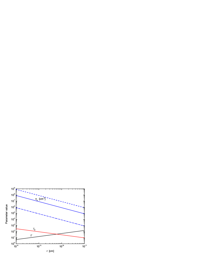
Figure 2: Dependence of the free model parameters of the X-ray emitting region: the bulk Lorentz factor, $\Gamma$ (black) the typical Lorentz factor of electrons, $\gamma_{e}$ (red) and the number density of electrons in the observer’s frame, $n_{e}$ (blue) on the radius of source, $r$. The solid, the dashed and the dash-dotted lines represent the averaged X-ray luminosity $3\times 10^{47}~{}{\rm erg~{}s^{-1}}$, the maximum luminosity $\sim 3\times 10^{48}\,{\rm erg\,s^{-1}}$ and the minimum luminosity $\sim 3\times 10^{45}\,{\rm erg\,s^{-1}}$, respectively. We assume that IC scattering of the radio photons are the main source of X-rays.

The X-ray luminosity varies in the range $\sim 3\times 10^{45}\,{\rm erg\,s^{-1}}$ — $\sim 3\times 10^{48}\,{\rm erg\,s^{-1}}$. This uncertainty leads to an uncertainty in the number density (or the total number of) electrons. However, the derived values of the bulk Lorentz factor and the typical Lorentz factor of electrons (Equations 4 and 6) are not affected by this uncertainty. In the results presented in Figure 2, we thus present three values of the number density (as a function of $r$), obtained by taking different observed fluxes of the X-rays: The solid blue line corresponds to the average X-ray flux, $3\times 10^{47}~{}{\rm erg~{}s^{-1}}$, while the dash and dash-dotted lines correspond to the maximum and minimum observed X-ray flux, respectively.

From the results of Figure 2 one can put several constraints on the X-ray emission zone: First, there is no strong constraint on the size of the emitting region, $r$. Any value in the range $10^{15}~{}{\rm cm}<r<10^{16}~{}{\rm cm}$, which is compatible with the size of the emission zone of the synchrotron photons, is acceptable. The main constraint originates from equation (6), as large radius implies large bulk Lorentz factor, since $\Gamma\simeq r^{1/2}/(2.1\times 10^{6})$. Thus, value of $r\approx 10^{16}$ cm imply $\Gamma\approx 50$, much larger than the value obtained for the radio emission zone. Even value of $r=10^{15}$ cm implies $\Gamma\approx 15$, inconsistent with the finding for the radio emitting zone. Thus, while the size of the radio and X-ray emitting regions can be comparable, the X-ray emitting region must propagate at much larger Lorentz factor than the radio emitting region. Second, the IC emitting electrons are not as hot as the radio emitting electrons. For $r\gtrsim 10^{15}$ cm, $\Gamma\gtrsim 15$, which, using equation (4) imply $\gamma_{e[IC]}\lesssim 100$. Third, the number density of the radiating electrons, $10^{4}{\rm\,cm^{-3}}\lesssim n\lesssim 10^{8}{\rm\,cm^{-3}}$ is comparable to the number density of the radio emitting particles, and is thus likely too high to be explained by compression of the external material. A similar conclusion holds for the total number of the radiating particles.

Thus, we conclude that while the two emission regions can have a comparable size, the X-ray emission zone must have a much larger Lorentz factor than the radio emission zone; moreover, the electrons in the X-ray emitting region must be colder than the electrons that emit at radio frequencies. Alternatively, the bulk motion may be similar, but only if the X-ray emitting region is at much smaller distance, $10^{12.5}$ cm. These results are summarized in Table LABEL:tab01. The numbers for the X-ray emission region in Table 1 are obtained by taking the average X-ray luminosity, $L_{x}=3\times 10^{47}\,{\rm erg\,s^{-1}}$.

Table 1: Summary of key properties of both radio and X-ray emission zones of Swift J164449.3+573451

	$R\,{\rm[cm]}$	$\Gamma$	$\gamma_{e}$	$n_{e}\,{\rm[cm^{-3}]}$	$N_{e}$
Radio emission
zone	$3\times 10^{15}-10^{16}$	$\lesssim 1.2$	$150-2000$	$10^{3.5}-10^{7.5}$	$10^{52}-10^{54.5}$
X-ray emission
zone	$10^{15}-10^{16}$	$15-50$	$30-100$	$10^{5}-10^{8}$	$10^{52}-10^{54.5}$
(alternative)	$10^{12.5}$	$\lesssim 1.2$	$\sim 1000$	$10^{9.5}$	$10^{47.5}$

Notes. — In the table, the model parameters $R$: source radius, $\Gamma$: bulk Lorentz factor, $\gamma_{e}$: typical Lorentz factor of relativistic electrons, $n_{e}$: number density of emitting electrons, and $N_{e}$: total number of electrons in the observer’s frame.

Similarly, although order-of-magnitude variations in brightness are seen in the X-rays, the detailed radio light curve does not reveal the coincident variations that would be expected for SSC (Zauderer et al., 2011; Levan et al., 2011). We therefore conclude that the X-ray emission must originate from a region separated than the radio emission region.

While observations made in the first few days cannot discriminate between the two alternatives for the X-ray emitting region, we show in §3 below that the re-brightening observed at radio flux after tens of days can be naturally explained as resulting from material collected by the X-ray emitting plasma, provided that it travels at $\Gamma\approx 10-20$. Thus, the first model, in which the X-ray emission region is separated from the radio emission region in velocity space is preferred. This leads us to a proposed two component jet, in which the fast, X-ray emitting material, is surrounded by a slower, radio emitting material. A cartoon demonstrating this model is shown in Figure 3.

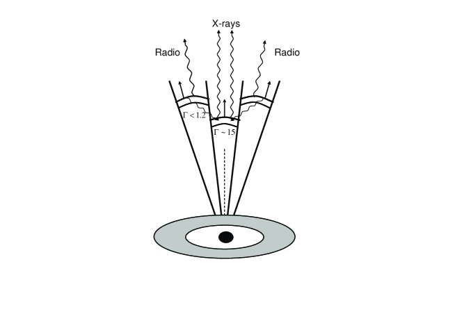
Figure 3: Sketch of geometrical configuration and emission regions for TDE Swift 1644+57. The inner jet has a Lorentz factor $\Gamma\approx 15$, and is responsible for the early times X-ray emission. The outer jet has Lorentz factor $\lesssim 1.2$, and is the source of the early times radio emission. As the inner jet propagates through the ISM it collects material and cools. Synchrotron emission from the collected material is the source of the re-brightening seen in radio frequencies after $\approx 30$ days.

2.3 Constraints on GeV emission

In the framework of the two-component jet model proposed here, a strong $\sim$ GeV flux is produced. This results from inverse Compton scattering of the X-ray photons produced in the inner jet by energetic electrons in the same region. Using the outflow parameters derived above (see Table LABEL:tab01), we find that the X-ray photons (of characteristic observed energy $\sim 10$ keV) will be upscattered to observed energies $\sim\gamma_{e}^{2}h\nu_{x}\sim 100$ MeV. Accordingly, the luminosity of this sub-GeV emission is expected to be $L_{\rm GeV}/L_{x}=Y=n_{e}\sigma_{T}r\gamma_{e}^{2}\gtrsim 10$, where $Y$ is Compton parameter. Using the observed X-ray luminosity $L_{x}\sim 3\times 10^{47}~{}{\rm erg/s}$, one can naively expect $L_{\rm GeV}\gtrsim 10^{48}~{}{\rm erg/s}$, which exceeds the limits set by Fermi (Burrows et al., 2011) by about two orders of magnitude.

This GeV emission, however, is strongly suppressed by annihilating with the X-ray photons, and cannot, therefore, be detected. Photons at $\sim 1$ GeV (observed energy) will annihilate with photons at observed energies in the X-ray band, of $\gtrsim 50$ keV (assuming bulk Lorentz factor $\Gamma\sim 15$). The (comoving) number density of these X-ray photons is $n_{x}^{\prime}\approx L_{x}/(4\pi r^{2}\Gamma^{2}c\langle\epsilon^{\prime}\rangle)\approx 7\times 10^{11}~{}{\rm\,cm^{-3}}$, where we have assumed $r\simeq 10^{15}$ cm, $\Gamma\approx 15$ and $\langle\epsilon^{\prime}\rangle\approx 3$ keV is the comoving energy of the X-ray photons. The optical depth for pair production is thus $\tau_{\gamma\gamma}\approx(r/\Gamma)n_{x}^{\prime}{\sigma}_{\gamma\gamma}=5$, where the cross section for $\gamma-\gamma$ annihilation is ${\sigma}_{\gamma\gamma}\sim 10^{-25}~{}{\rm cm}^{2}$. This attenuation can explain the lack of detection of GeV photons by Fermi (Burrows et al., 2011).

We further point that $\approx 100$ MeV photons annihilate with photons at $\sim 500$ KeV, whose flux may be lower than that of 50 keV photons. However, the Fermi upper limits are obtained on the integrated flux between 100 MeV and 10 GeV; Moreover, as the XRT bandwidth is limited to below 150 keV, no observational constraints exist on the number density of photons, hence on the optical depth for annihilation at these energies.

3 Late time radio evolution

The two component jet model presented above has a distinct prediction. As the plasma expands into the interstellar material (ISM), it collects material, slows and cools. This situation is similar to the afterglow phase in GRBs (e.g., Zhang & MacFadyen, 2009; Granot & Piran, 2012; van Eerten & MacFadyen, 2012; van Eerten, 2013, and references therein). Thus, using similar assumptions, one can predict the late time synchrotron emission from the decelerating plasma. One notable difference from GRB afterglow, though, is that the X-ray emitting plasma is mildly relativistic, while the radio emitting plasma is trans-relativistic. Thus, when calculating the dynamics, one cannot rely on the ultra-relativistic scheme (Blandford & McKee, 1976), but has to consider the transition to the Newtonian regime.

3.1 Dynamics and radiation from an expanding jet

The dynamics of plasma expanding through the ISM is well studied in the literature (Blandford & McKee, 1976; Katz & Piran, 1997; Chiang & Dermer, 1999; Piran, 1999; Huang et al., 1999; van Paradijs et al., 2000; Pe’er, 2012; Nava et al., 2012). Here we briefly review the basic theory, which we then utilize in calculating the expected late time radio emission from TDE Swift 1644+57.

We assume that by the relevant times (tens of days), the reverse shock had crossed the plasma, and thus only the forward shock exists. The evolution of the bulk Lorentz factor of the expanding plasma is given by (Pe’er, 2012)

$$\frac{{\rm d}\Gamma}{{\rm d}m}=-\frac{\hat{\gamma}\left(\Gamma^{2}-1\right)-\left(\hat{\gamma}-1\right)\Gamma\beta^{2}}{M+\epsilon m+\left(1-\epsilon\right)m\left[2\hat{\gamma}\Gamma-\left(\hat{\gamma}-1\right)\left(1+\Gamma^{-2}\right)\right]}.$$ (7)

Here, $M$ is the mass of the ejected matter, $m$ is the mass of the collected ISM, $\Gamma$ is the bulk Lorentz factor of the flow, $\hat{\gamma}$ is the adiabatic index and $\epsilon$ is the fraction of the shock-generated thermal energy that is radiated ($\epsilon=0$ in the adiabatic case and $\epsilon=1$ in the radiative case). Note that equation (7) holds for any value of $\Gamma$, both in the ultra-relativistic ($\Gamma\gg 1$) and the sub-relativistic ($\beta\ll 1$) limits.

Under the assumption of constant ISM density, the collected ISM mass is related to the distance ${\rm d}R$ and observed time ${\rm d}t$ via

$$\begin{array}[]{lcl}{\rm d}m&=&4\pi R^{2}n_{\rm ISM}m_{\rm p}{\rm d}R;\\ {\rm d}R&=&\Gamma\beta c\left(\Gamma+\Gamma\beta\right){\rm d}t=\frac{\beta}{1-\beta}c{\rm d}t,\end{array}$$ (8)

where $m_{p}$ is the proton’s rest mass and $n_{\rm ISM}$ is the ISM density. In deriving the second line in equation (8), we have explicitly assumed that the observed photons are emitted from a plasma that propagates towards the observer. A more comprehensive calculation which considers the integrated emission from different angles to the line of sight results in a similar solution, up to a numerical factor of a few (Waxman, 1997; Pe’er & Wijers, 2006).

In order to predict the synchrotron emission, one needs to calculate the magnetic field, $B$ and characteristic electron’s Lorentz factor, $\gamma_{\rm el}$. This calculation is done as follows. By solving the shock jump conditions, one gets the energy density behind the shock (Blandford & McKee, 1976),

$$u_{2}=\left(\Gamma-1\right)\frac{\hat{\gamma}\Gamma+1}{\hat{\gamma}-1}n_{\rm ISM}m_{\rm p}c^{2}~{}.$$ (9)

Equation (9) is exact for any velocity, including both the ultra-relativistic and the Newtonian limits. A useful approximation for the adiabatic index is $\hat{\gamma}=(4\Gamma+1)/(3\Gamma)$ (e.g., Dai et al., 1999). In the ultra-relativistic limit, $\Gamma\gg 1$, $\hat{\gamma}=4/3$ and equation (9) takes the form $u_{2}\approx 4\Gamma^{2}n_{\rm ISM}m_{\rm p}c^{2}$; While in the Newtonian limit, $\beta\ll 1$ and $\hat{\gamma}=5/3$, equation (9) becomes $u_{2}\approx 2\beta^{2}n_{\rm ISM}m_{\rm p}c^{2}$.

The shock-generated magnetic field assumes to carry a fraction $\epsilon_{\rm B}$ of the post-shock thermal energy, $B^{2}/8\pi=\epsilon_{\rm B}u_{2}$,

$$B=\left\{\begin{array}[]{ll}(32\pi\epsilon_{\rm B}n_{\rm ISM}m_{\rm p}c^{2})^{1/2}\Gamma&({\rm relativistic~{}limit}),\\ \left(16\pi\epsilon_{\rm B}n_{\rm ISM}m_{\rm p}c^{2}\right)^{1/2}\beta&({\rm Newtonian~{}limit}).\end{array}\right.$$ (12)

Similarly, a constant fraction $\epsilon_{\rm e}$ of the post-shock thermal energy is assumed to be carried by energetic electrons, resulting in $\gamma_{\rm el}m_{\rm e}c^{2}=\epsilon_{\rm e}(u_{2}/n_{2})$, where the number density in the shocked region is $n_{2}=n_{\rm ISM}(\hat{\gamma}\Gamma+1)/(\hat{\gamma}-1)$. This leads to

$$\gamma_{\rm el}=\left\{\begin{array}[]{ll}\epsilon_{\rm e}\Gamma\left(\frac{m_{\rm p}}{m_{\rm e}}\right)&({\rm relativistic~{}limit}),\\ \epsilon_{\rm e}\frac{\beta^{2}}{2}\left(\frac{m_{\rm p}}{m_{\rm e}}\right)&({\rm Newtonian~{}limit}).\end{array}\right.$$ (13)

In order to calculate the observed peak frequency and flux, we discriminate between two cases:

(i) In the optically thin emission, $\nu_{a}<\nu_{m}$, i.e., $\tau_{\nu_{m}}<1$, the peak synchrotron frequency is $\nu_{p}^{\rm ob}=\nu_{m}^{\rm ob}=(3/4\pi)(q_{e}B/m_{e}c)\gamma_{\rm el}^{2}\Gamma$ and the peak flux $F_{\nu_{p}}=F_{\nu_{m}}\approx(N_{e}/4\pi d_{L}^{2})(2\sigma_{T}m_{e}c^{2}B\Gamma/9q_{e})$ (e.g., Sari et al., 1998). Here, $d_{L}$ is the luminosity distance and $N_{e}\propto R^{3}$ is the total number of radiating electrons (originating both at the explosion, as well as collected ISM). In the limit where the total number of swept-up ISM material is much larger than the original ejected material, analytic scaling laws can be obtained in the ultra-relativistic and Newtonian limits. In the relativistic regime, $\Gamma\gg 1$, $\Gamma\propto t^{-3/8}$ and $R\propto t^{1/4}$, and thus $\nu_{p}^{\rm ob}\propto t^{-3/2}$ and $F_{\nu_{p}}\propto t^{0}$. On the other hand, in the Newtonian limit, $\beta\propto t^{-3/5}$ and $R\propto t^{2/5}$, one finds $\nu_{p}^{\rm ob}\propto t^{-3}$ and $F_{\nu_{p}}\propto t^{3/5}$.

The temporal evolution of the self absorption frequency is calculated using the relation between $\nu_{a}$ and $\nu_{m}$ (Equation 2), the scaling laws of $B$ and $\gamma_{el}$ derived in Equations 12 and 13, the relation $N_{e}\propto R^{3}$ and the scaling laws of $R$ and $\Gamma$. Using the results of Equation 2, one can write $\nu_{a}\propto\nu_{p}^{\rm ob}N_{e}^{3/5}R^{-6/5}B^{-3/5}\gamma_{el}^{-3}$. In the ultra-relativistic case, $B\propto\Gamma$, $\gamma_{el}\propto\Gamma$, $\Gamma\propto t^{-3/8}$ and $R\propto t^{1/4}$, and therefore $\nu_{a}\propto t^{0}$, namely time-independent. In the other extreme of Newtonian motion, $B\propto\beta$, $\gamma_{el}\propto\beta^{2}$, $\beta\propto t^{-3/5}$ and $R\propto t^{2/5}$, leading to an increase of the self absorption frequency with time, $\nu_{a}\propto t^{6/5}$.

(ii) In the optically thick regime, $\nu_{a}>\nu_{m}$, i.e., $\tau_{\nu_{m}}>1$, the observed peak frequency $\nu_{p}$ and the peak flux $F_{\nu_{p}}$ are at the self absorption frequency, $\nu_{a}$. For a power law distribution of electrons above $\gamma_{\rm el}$ with power law index $p$, these are given by

$$\begin{array}[]{rcl}\nu_{p}^{\rm ob}=\nu_{a}^{\rm ob}=\nu_{m}^{\rm ob}\tau_{\nu_{m}}^{2/(p+4)}&=&\frac{3}{4\pi}\frac{q_{e}B}{m_{\rm e}c}\gamma_{\rm el}^{2}\Gamma\tau_{\nu_{m}}^{2/(p+4)}~{},\\ F_{\nu_{p}}=F_{\nu_{m}}\left(\frac{\nu_{a}}{\nu_{m}}\right)^{-\frac{p-1}{2}}&=&F_{\nu_{m}}\tau_{\nu_{m}}^{-\frac{p-1}{p+4}}\approx\frac{N_{\rm e}}{\rm 4\pi d_{L}^{2}}\frac{2}{9}\frac{\sigma_{\rm T}m_{\rm e}c^{2}}{q_{e}}B\Gamma\tau_{\nu_{m}}^{-\frac{p-1}{p+4}}~{}.\end{array}$$ (14)

The optical depth at $\nu_{m}$, $\tau_{\nu_{m}}$ is calculated as follows. We first point out that the comoving number density of the electrons in the shocked plasma frame is $n_{2}\simeq 4\Gamma n_{\rm ISM}$. Using equation (6.52) in Rybicki & Lightman (1979), we find that $\tau_{\nu_{m}}=\alpha_{\nu_{m}}(R/\Gamma)=f(p)n_{\rm ISM}B^{-1}\gamma_{\rm el}^{-5}R$ (see also Pe’er & Waxman, 2004). Here, $f(p)=(p-1)(8\pi\sqrt{3}q_{e}/9)2^{p/2}\Gamma((2p+2)/12)\Gamma((3p+22)/12)$ is a function of the power law index, $p$ of the accelerated electrons above $\gamma_{\rm el}$, and $\Gamma(x)$ is $\Gamma$ function of argument $x$. Using this result in equation (14), one can obtain analytic scaling laws for the temporal evolution of $\nu_{p}^{\rm ob}$ and $F_{\nu_{p}}$ in both the ultra-relativistic and Newtonian limits, in a similar way to the derived expressions in the optically thin limit above. In the relativistic regime, $\nu_{p}^{\rm ob}\propto t^{-(3p+2)/2(p+4)}\propto t^{-2/3}\,(p=2)$ and $F_{\nu_{p}}\propto t^{5(1-p)/2(p+4)}\propto t^{-5/12}\,(p=2)$. In the Newtonian limit, one finds $\nu_{p}^{\rm ob}\propto t^{(2-3p)/(p+4)}\propto t^{-2/3}\,(p=2)$ and $F_{\nu_{p}}\propto t^{(47-32p)/5(p+4)}\propto t^{-17/30}\,(p=2)$.

The scaling laws presented above are derived under the assumption that the origin of the magnetic field and the source of energy of energetic particles originates from randomization of the kinetic energy at the shock front. As such, these scaling laws are valid for the collected ISM plasma. However, we argue that similar scaling laws hold for the plasma originally ejected in the jet, at least at late times (after a few days) when the ejecta radii is much larger than its original radii, and the motion becomes self similar.

The ejected material and the collected ISM are separated by a contact discontinuity. By definition, the energy densities at both sides of the discontinuity are the same. Thus, using the common assumption that constant fractions of the energy density are used in generating magnetic fields and accelerating particles, one must conclude similar values at both sides of the contact discontinuity. Moreover, the contact discontinuity is unstable, implying a mixture of materials at both its sides (Duffell & MacFadyen, 2014). Thus, even if the values of the physical parameters were initially different at both sides of the discontinuity, we expect them to average out at late times.

3.2 Radiative cooling of the electrons

In the calculation presented in §3.1 (in particular, equation (13) above), we considered heating of the ISM plasma as it crosses the shock front. Once the ISM particles cross the shock front, they lose their energy by radiative cooling. Hence, their typical Lorentz factor $\gamma_{\rm el}$ decreases with time. Similarly, the original ejected material from the tidally disrupted star cools with time.

Within the context of our double jet model, this cooling has a more pronounced effect on the lightcurve originating from the outer jet, that is responsible for the early time radio emission. This is because this region is composed of a dense plasma, that propagates at trans-relativistic velocities (see Table LABEL:tab01). The contribution of the swept-up ISM material to the emission during the first $\sim$ month from this region is therefore minor, as opposed to the contribution of the collected ISM to the emission from the inner jet. This can be seen by noting that during Newtonian expansion, $R\propto t^{2/5}$. Thus, between five and thirty days, the radius of the radio emitting region is increased by a factor $\approx 2$, and therefore cannot exceed $\approx 2\times 10^{16}$ cm. As a result, unless the ISM density is much larger than $\sim 10^{3}\,\rm{cm^{-3}}$, contribution from the collected ISM to the emission from the outer jet is subdominant.

Although the total number of collected ISM particle within the first month is considerably smaller than the number of particle that existed initially in the outer jet, the collection of the ISM material caused the jet to slow. Our underlying assumption is that by 5 days, the outer jet have already reached its self-similar phase, whose scaling laws we derived above. The slowing down and expansion of the jet leads to a decrease in the energy density, hence of both the photon and magnetic field with time. This, in turn, modifies the electrons cooling rate. The cooling of the electrons, in turn, leads to a decay of the radio emission (from the electrons that initially exist in the outer jet). Here we calculate the temporal evolution of the electron’s Lorentz factor, resulting from this radiative decay. We stress that in the framework of our model, both the initially ejected outer jet material and collected ISM material radiate, under similar conditions (same magnetic field, etc.). While this may only be a crude approximation (e.g., Duffell & MacFadyen, 2014), the results obtained are consistent with the data, implying that this assumption may be valid.

The radio emitting electrons cool due to synchrotron and inverse Compton scattering. The radiated power from a relativistic electron with Lorentz factor $\gamma_{\rm el}$ is $P=P_{\rm syn}+P_{\rm IC}=(4/3)c\sigma_{T}\left(U_{B}+U_{\rm ph}\right)\gamma_{\rm el}^{2}$, where $U_{B}$ and $U_{\rm ph}$ are the magnetic and radiative field energy densities, respectively.

Both $U_{B}$ and $U_{\rm ph}$ decrease with radius (and time). As discussed in §3.1 above, during the Newtonian expansion phase $B\propto\beta\propto t^{-3/5}$ (see equation (12)), and thus $U_{B}\propto t^{-6/5}$. Similarly, $U_{\rm ph}=L/(4\pi R^{2}\Gamma^{2}c)$, where the luminosity is $L\propto N_{e}\gamma_{\rm el}^{2}B^{2}\Gamma^{2}\propto\beta^{6}\propto t^{-18/5}$ (assuming that most radiative particles are from the original ejecta). This leads to $U_{\rm ph}\propto t^{-22/5}$, namely the IC component decreases much faster than the synchrotron component.

We can therefore write $P\approx(4/3)c\sigma_{T}U_{B,0}(t/t_{0})^{-6/5}\gamma_{\rm el}^{2}$, where $U_{B,0}$ is the magnetic field energy density at fiducial time, $t_{0}$ which is taken in the calculations below to be five days (observed time). The characteristic particles Lorentz factor at any given time $t>t_{0}$ is given by

$$\gamma_{\rm el}(t)=\frac{\gamma_{\rm el,0}}{1+{20\over 3}{\sigma_{T}\over m_{e}c}U_{B,{0}}\gamma_{\rm el,0}t_{0}\left[1-\left(t/t_{0}\right)^{-1/5}\right]}~{},$$ (15)

where $\gamma_{\rm el,0}$ is the electron’s Lorentz factor at $t_{0}$. The temporal evolution of the electron’s Lorentz factor and the decay law of the magnetic field allow calculation of the late time evolution of both the peak radio frequency and peak radio flux from the outer jet region.

3.3 Lateral expansion

The temporal evolution of the observed peak frequency and peak flux were derived above under the assumption of spherical expansion. In a jetted outflow, initially the sideways expansion can be neglected; however, once the outflow decelerates to $\Gamma\approx\theta_{j}^{-1}$ (where $\theta_{j}$ is the initial jet opening angle), lateral expansion becomes significant. The flow expands sideways during its trans-relativistic phase, which lasts a typical observed time of few - few hundred days before asymptoting to a spherical, Newtonian expansion described by the Sedov-Taylor solutions discussed above (Livio & Waxman, 2000; van Eerten et al., 2011; Wygoda et al., 2011).

In a jetted outflow with $\theta_{j}\ll 1$, the true jet energy is $E_{j}\approx E_{iso}\theta_{j}^{2}/2$. One can derive the temporal evolution of the peak frequency and peak flux during the lateral expansion phase, by noting that during this phase, the jet opening angle scales with the radius roughly as $\theta\propto R$, irrespective of the initial jet opening angle, $\theta_{j}$ (van Eerten et al., 2011). Conservation of energy implies that

$$E_{j}\propto R^{3}\theta^{2}u_{2}\propto R^{5}\Gamma^{2}\beta^{2}=Const,$$ (16)

where we used the fact that the energy density behind the shock front, $u_{2}\propto\Gamma^{2}\beta^{2}$ (see Equation 9), which is valid for expansion into $r$-independent ISM density profile.

In the Newtonian regime, $\beta\ll 1$, which is a good approximation during this phase, one thus finds that the temporal evolution of the radius and velocity are $R\propto t^{2/7}$ and $\beta\propto t^{-5/7}$. Using these results in Equations 12 and 13, one finds $B\propto\beta\propto t^{-5/7}$ and $\gamma_{\rm el}\propto\beta^{2}\propto t^{-10/7}$. Moreover, the total number of radiating electrons collected from the ISM is $N_{e}\propto R^{3}\theta^{2}\propto R^{5}\propto t^{10/7}$.

Repeating the same arguments as in section 3.1 above, one finds that in the optically thin regime, $\nu_{p}^{\rm ob}\propto B\gamma_{\rm el}^{2}\Gamma\propto t^{-25/7}$ and $F_{\nu_{p}}\propto N_{e}B\propto t^{5/7}$. In the optically thick regime, $\nu_{p}^{\rm ob}\propto\nu_{a}^{\rm ob}\propto\Gamma B^{{P+2\over P+4}}\gamma_{\rm el}^{{2p-2\over p+4}}R^{{2\over p+4}}\propto t^{14-25p\over 7(p+4)}\propto t^{-6/7}$, where the last equality holds for $p=2$. Similarly, in this regime, $F_{\nu_{p}}\propto N_{e}R^{-{p-1\over p+4}}B^{2p+3\over p+4}\gamma_{\rm el}^{5(p-1)\over p+4}\Gamma\propto t^{77-52p\over 7(p+4)}\propto t^{-9/14}$ (for $p=2$).

4 Interpretation of the late time radio emission of Sw J1644+57

The temporal evolution of the radio flux and peak radio frequency of Sw J1644+57 up to 582 days from the initial outburst are presented in Figures 4, 5 (data taken from Berger et al., 2012; Zauderer et al., 2013). Three separate regimes are identified in both figures: (I) At early times, $\lesssim 30$ days, the flux decreases from $\sim 40~{}{\rm mJy}$ at $\sim 5$ days to $\sim 15~{}{\rm mJy}$ at $\sim 30$ days. During this period, $\nu_{p}^{\rm ob}$ rapidly decays, with a decay law consistent with $\nu_{p}^{\rm ob}\propto t^{-\alpha}$ and $\alpha\approx 2.0$. (II) Between $30-100$ days, the flux increases by a factor of $\sim 1.8$ (from $\sim 20~{}{\rm mJy}$ to $\sim 35~{}{\rm mJy}$). At the beginning of this epoch, at $t^{\rm ob}\sim 30-45$ days, the radio peak frequency $\nu_{p}^{\rm ob}$ increases by a factor of a $few$, while during the rest of this epoch it shows a similar decay law as is seen at early times, $\nu_{p}^{\rm ob}\propto t^{-\alpha}$ with $\alpha\approx 2.0$. (III) Finally, at very late times, $\gtrsim 100$ days, the flux decays again. This decay is accompanied by a slow decay in the peak radio frequency, much slower than the decay observed at earlier phases. We point out that the increase in the radio flux observed at epoch (II) led Berger et al. (2012) to suggest that late time energy injection may take place.

Based on the discussion presented in the previous sections, we suggest the following interpretation to the late time radio emission of Sw J1644+57: (I) During the early decay phase, $t^{\rm ob}<30$ days, the emission is dominated by synchrotron radiation from the same electrons that emitted the radio emission at early times; this is the outer jet component in our model (see Figure 3). This emission is thus a continuation of the emission observed at early times. The observed decay of both the flux and peak frequency is due to the decreasing of magnetic field and the radiative cooling of these electrons. (II) At $t^{\rm ob}\approx 30$ days, there is a transition: the inner jet plasma, that originally emitted the X-ray photons, expands into the ISM, collects ISM material and cools. At this time, synchrotron emission from this plasma becomes the dominant component at radio frequencies. Initially, the inner jet propagates at relativistic speeds, with $\Gamma\gtrsim 15$ (see discussion in §2.2 and Table LABEL:tab01). However, as it propagates into the ISM, the plasma collects material from the surrounding ISM and slows; the collected material contributes to the radio emission, resulting in an increase in the radio flux. (III) Finally, at $t^{\rm ob}\sim 100$ days, the emission becomes optically thick (self absorption frequency is larger than the peak frequency), which causes the late time decay.

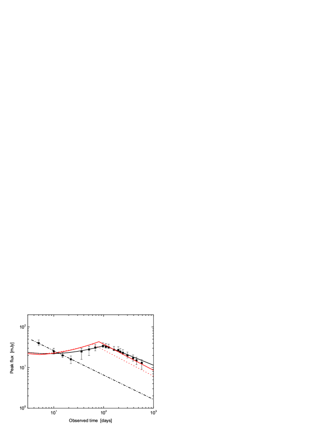
Figure 4: Temporal evolution of peak flux of the radio emission of Swift 1644+57. Data is taken from Berger et al. (2012) and Zauderer et al. (2013). The vertical bars represent the uncertainties in determining the exact value of the peak flux from the data provided by Berger et al. (2012) and Zauderer et al. (2013), and not statistical errors, which are not publicly available. Dash-dotted line is the contribution of the outer (slower) jet, while black solid line is the contribution from the inner (faster) jet in the spherical scenario. The red lines represent fits to the data obtained when lateral expansion is considered, when the inner jet Lorentz factor reaches $\Gamma\leq 2$. The red solid line assumes the initial parameters described in §4.3, while the red dotted line uses the same initial parameters as in the spherical scenario. As the inner jet propagates into the ISM, it collects material and cools; thus, after $\sim 30$ days, radio emission from this region dominates the radio flux. At $\sim 100$ days, the peak flux enters the optically thick regime ($\tau_{\nu_{p}}>1$), which causes the decay seen at these times. The values of the free model parameters used are presented in the text.

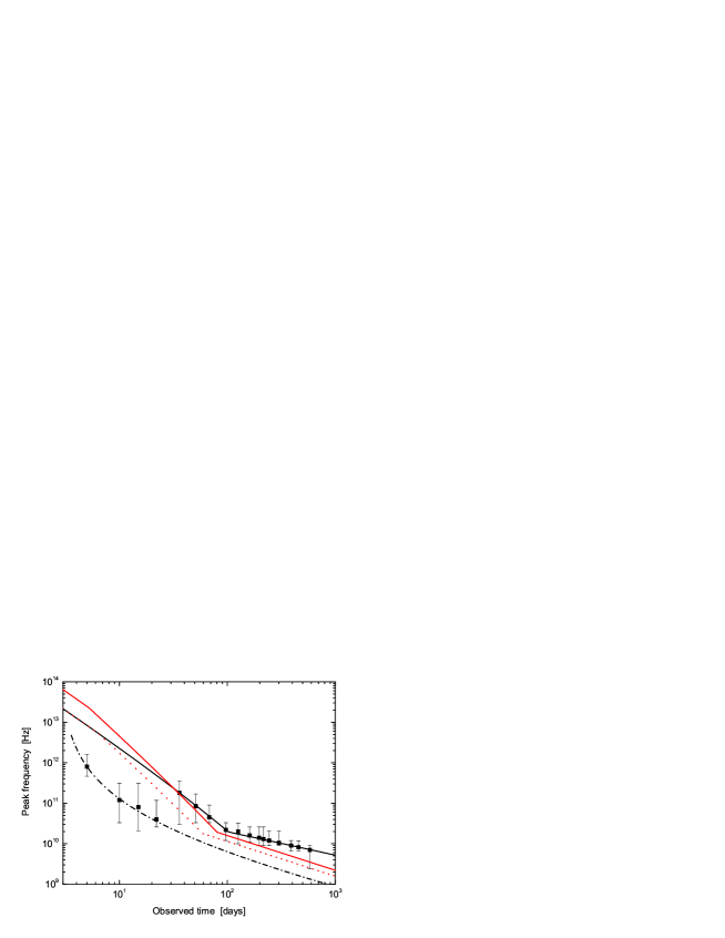
Figure 5: Temporal evolution of peak frequency for the radio emission of Swift 1644+57. Observed data taken from Berger et al. (2012) and Zauderer et al. (2013). Lines have the same meaning as in Figure 4. Three distinctive regimes are clearly seen.

Fits to the temporal evolution of the peak radio frequency and peak flux are shown in Figures 4 and 5. The black solid curves represent fits done using spherically symmetric scenario, while in the red solid and dotted curves we fit the data using the lateral expansion scaling laws derived in §3.3, which are used when the Lorentz factor drops below $\Gamma\leq 2$.

Consider first the spherical scenario, presented by the black solid curves. In producing the fits, we use the following parameters, which match the early and late time properties of the flow. For the outer jet, we use initial expansion radius (at observed time $t_{0}^{\rm ob}=5$ days) $R_{0}=10^{16}$ cm. The typical electron’s Lorentz factor is taken to be $\gamma_{\rm el,0}=190$, magnetic field $B_{0}=4.5$ G, and initial bulk Lorentz factor $\Gamma(t_{0}^{\rm ob})\simeq 1.18$. These values correspond to $\epsilon_{\rm e}\approx 0.58$ and $\epsilon_{\rm B}\approx 0.13$, and imply total number of radiating particles $N_{e}(t_{0})=1.25\times 10^{53}$. These values are consistent with the findings in §2.1 (see Table LABEL:tab01). These parameters result in initial peak synchrotron frequency $\nu_{p,0}^{\rm ob}=8.0\times 10^{11}$ Hz, and peak observed flux $F_{\nu_{p},0}=39.4$ mJy.

For the inner jet, we find that the best fit is obtained when using initial bulk Lorentz factor $\Gamma(t^{\rm ob}=100~{}\rm{s})=17$, $\epsilon_{\rm e}=0.54$, $\epsilon_{\rm B}=0.54$ and $r(t^{\rm ob}=100~{}\rm{s})\simeq 1.2\times 10^{15}$ cm. We point out that the value of $\epsilon_{B}$ is not constrained by early X-ray data. Moreover, here the collected ISM plays a significant role. Thus, we could constrain the ISM density to be $n_{\rm ISM}=2.7~{}{\rm cm^{-3}}$. We further assume that the shocked ISM have a power law distribution above $\gamma_{\rm el}$ with power law index $p=2$. When calculating the dynamics in equation (7), we consider adiabatic expansion, namely $\epsilon=0$.

4.1 The transition at 30 days

Within the context of our model there are four separated regimes that contribute to the emission. (I) Emission from matter ejected at the outer (slower) jet dominates before $\sim 30$ days, as is shown by the fits; (II) contribution from ISM material collected by the outer jet, which is sub-dominant, as the amount of ISM material collected in the first month is significantly smaller than the material that originated in the outer jet (see discussion in §3.2); (III) contribution of emission from material originated in the inner jet (which, as we show below, can not be constrained by the data); and (IV) contribution of ISM material collected by the inner jet, which becomes the dominant source of radio emission after $\sim 30$ days, and causes the rise in the radio flux observed at later times.

At $\approx 30$ days a transition occurs, as contribution from the inner jet (and ISM material collected by it) becomes the dominant source of radio emission. Using equations 7, 8, one finds that at that time, the inner jet is at radius $\sim 4.2\times 10^{17}$ cm and the number of the collected ISM protons is $\sim 8.4\times 10^{53}$, which is much larger than the number of particles that initially existed in the jet, $N_{\rm initial}=5.5\times 10^{52}$ in the fits presented. Therefore, the contribution of the collected ISM to radio emission from the inner jet is dominant (under the assumption of similar magnetic fields and similar Lorentz factor of the radiative electrons at both the ejected plasma and the collected ISM).

We note that a significant deceleration of the inner jet occurs much earlier. The deceleration becomes significant when the collected mass from the ISM is $\approx N_{\rm initial}m_{p}/\Gamma$ (e.g., Pe’er, 2012). This occurs at radius $R\sim 7\times 10^{16}$ cm, corresponding to observed time $R/(\Gamma^{2}c)\approx 8000$ s (assuming initial inner jet properties $\Gamma=17$ and $N_{\rm initial}=5.5\times 10^{52}$, as discussed above and in Figure 2). Therefore, a significant decrease in the inner jet Lorentz factor occurs already after a few hours. Using Equations 7, 8, we find that the inner jet Lorentz factor drops to $\Gamma\leq 2$ after $\approx 6$ days (observed time). At this epoch, lateral expansion may be significant; see discussion in §4.3 below.

The collected ISM contributes to the radio emission from the inner jet. Its contribution to the radio flux becomes comparable to that of the outer jet after $\gtrsim 10$ days, and dominant after $\sim 30$ days (see Figures 4, 5). At early times, however, the radio emission from the inner jet peaks at higher frequencies than those observed (see Figures 5 and 6). Figure 6 shows the temporal evolution of the three characteristic synchrotron frequencies: peak frequency $\nu_{m}$, self absorption frequency $\nu_{a}$ and cooling frequency, $\nu_{c}$ of emission from the inner jet. In the figure we use the same parameters as of the spherical scenario discussed above, i.e., $\Gamma_{\rm initial}=17$, $N_{\rm initial}=5.5\times 10^{52}$ and $n_{\rm ISM}=2.7~{}{\rm cm}^{-3}$. For example, at $\sim 20$ days, emission from the inner jet is expected to be peaked at $\sim 6\times 10^{11}$ Hz, with peak flux of $F_{\nu_{p}}\approx 20$ mJy. Available data at these times is limited to lower frequencies, $\leq 230$ GHz (Berger et al., 2012). The observed flux at 230 GHz, $\approx 10$ mJy, is lower than the expected flux at the peak frequency of $\sim 600$ GHz, as it should; It is in agreement with the expectations from synchrotron theory, $F_{\nu}/F_{\nu_{p}}=(\nu/\nu_{p})^{1/3}$ for $\nu_{a}<\nu<\nu_{p}$. Since at an even earlier times the peak flux of radio emission from the inner jet is at higher frequencies (see Figure 6), its contribution at the flux at the observed bands of 230 GHZ and below is further reduced.

At $\sim 30$ days, the peak frequency from the inner jet (And the ISM material collected by it) is $\nu_{m}^{\rm ob}\approx 2.5\times 10^{11}$ Hz and the self-absorption frequency is $\nu_{a}\approx 1.0\times 10^{10}$ Hz, namely the radio emission is in the optically thin regime (see Figure 6). We point out that these results are, in fact not far from the fits done by Berger et al. (2012) (see their table 2) for that time epoch, and therefore our model can equally well fit the existing spectrum (Figure 2 in Berger et al., 2012).

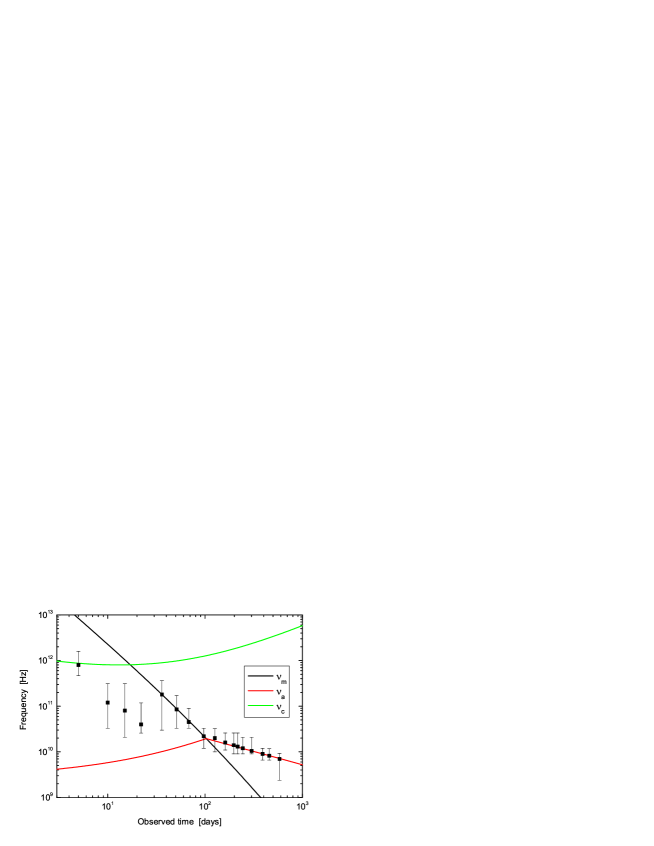
Figure 6: Temporal evolution of characteristic synchrotron frequencies: peak frequency $\nu_{m}$, self absorption frequency $\nu_{a}$ and cooling frequency, $\nu_{c}$ of emission from the inner jet, are plotted on top of the data. At the epoch 30-100 days, the emission is in the optically thin region, while at $t^{\rm ob}>100$ days it is in the optically thick regime. In producing the figure, we used the same parameters as in the spherical scenario, namely $\Gamma_{\rm initial}=17$, $N_{\rm initial}=5.5\times 10^{52}$ and $n_{\rm ISM}=2.7~{}{\rm cm}^{-3}$.

4.2 The transition at 100 days

The peak emission frequency (From the inner jet) drops faster than the self absorption frequency (see discussion in section 3.1 above, and Figure 6). At observed time $t^{\rm ob}=100$ days, the radio emission becomes optically thick, implying a change in the temporal decay of the observed peak flux and peak frequency, which are consistent with observations.

Using Equations 7, 8, we find that at observed time $t^{\rm ob}=100$ days, the inner jet reaches radius $R\sim 6.0\times 10^{17}~{}{\rm cm}$, with bulk Lorentz factor $\Gamma\sim 1.15$. At this time, the magnetic field is $B\sim 0.19$ G and the characteristic electrons Lorentz factor is $\gamma_{\rm el}\approx 150$. These result in $\nu_{p}^{\rm ob}=2.06\times 10^{10}$ Hz and $F_{\nu_{p}}=34.4$ mJy. However, at this time, $\tau_{\nu_{p}}\approx 1$, which implies that from this time onward synchrotron radiation is in the optically thick regime, and its late time properties are described by equations (14). The black solid lines in Figures 4, 5 represent the expected peak frequency and flux in the optically thin region at early times, and optically thick regions at $t^{\rm ob}>100$ days.

It should be emphasized that the fits presented here are different than those used by Berger et al. (2012) and Zauderer et al. (2013). In these works, spectral fits for the long-term radio data (up to $\sim$ 582 days) was done based on the formulae of the synchrotron spectrum model described in Metzger et al. (2012), or equation 4 in Berger et al. (2012). These, in turn, assume relativistic motion, $\Gamma\gg 1$. The obtained values of the fitted parameters vary with time; variation of the luminosity had led Berger et al. (2012) to propose late time energy injection. Furthermore, Berger et al. (2012) found $\nu_{a}<\nu_{m}$ even at late times. However, we point out that in their fits, they find $\nu_{a}\approx\nu_{m}$ at these epoch (see their table 2). Since the spectra at high frequencies $\nu\gg\max\{\nu_{a},\nu_{m}\}$ and at low frequencies, $\nu\ll\min\{\nu_{a},\nu_{m}\}$ is similar in the optically thin and optically thick cases, it is of no surprise that our model is also capable of reproducing the spectra.

In our model the late time radio emission after $\sim 30$ days originates from the interaction between the inner jet with ISM. Using the initial mass and bulk Lorentz factor of inner jetted outflow obtained by the analysis for the early X-rays in §2, we obtain good fits to the late time radio data presented in Figures 4, 5, without the need for late energy injection.

4.3 Lateral Expansion

We next consider a scenario in which lateral expansion takes place. These are shown by the red solid and dotted curves in Figures 4, 5. Such an expansion will take place once a jetted outflow slows down to $\Gamma\sim 1/\theta_{j}$. Since the initial jet opening angle $\theta_{j}$ is not constrained by the data, we cannot evaluate the significance of this effect. We therefore rely on the results of the recent simulations carried by (van Eerten et al., 2012), which indicate that sideways expansion becomes significant for $\Gamma\simeq 2.0$. Thus, in our fittings, the lateral expansion is considered when the Lorentz factor of the inner jet drops below 2. As explained above, this is expected after $\approx 6$ days (observed time).

When fitting the data, we use the scaling laws described in §3.3 to calculate the fits for temporal evolution of the peak radio frequency and peak flux after $\sim 30$ days. We make two fits to the data, shown by the red solid and red dotted lines in Figures 4 and 5. In the solid curve, we use the physical parameters $\Gamma(t_{0}^{\rm ob})=15$, $\epsilon_{\rm e}=0.84$, $\epsilon_{\rm B}=1.65$, $n_{\rm ISM}=2.6~{}{\rm cm}^{-3}$ and $r(t_{0}^{\rm ob})\simeq 1.0\times 10^{15}$ cm. We find that at observed time $t^{\rm ob}\approx 81$ days, the radio emission enters the optically thick regime with peak frequency $\nu_{p}^{\rm ob}=1.92\times 10^{10}$ Hz and peak flux $F_{\nu_{p}}=43.4$ mJy. At this time, the outflow reaches radius $R\sim 3.63\times 10^{17}~{}{\rm cm}$, with bulk Lorentz factor $\Gamma\sim 1.074$, magnetic field $B\sim 0.25$ G and characteristic electrons Lorentz factor $\gamma_{\rm el}\approx 127$.

In order to estimate the sole effect of the lateral expansion, we show in the red dotted curve the results of the fit made using similar parameters to those adopted in the spherical scenario, with lateral expansion taking place for $\Gamma\leq 2$. The results of the fits indicate that lateral expansion has a minor effect on the obtained data.

We can thus conclude that the results presented in Figures 4 and 5 indicate that both the spherical expansion and the sideways expansion scenarios enable us to obtain good fits to the late times radio data, within the context of the two component jet model proposed here. Moreover, we find that in both scenarios, similar values of the free model parameters are obtained.

5 Conclusions and Discussions

In this paper, we studied the early and late time emission of the TDE Sw J1644+57, both at radio and X-ray frequencies. Based on our analysis, we propose a two-component jet model (see Figure 3) that fits the observations. Our model contains both dynamical and radiative parts, and give a satisfactory interpretation for the origin of both the early time X-ray and radio emission, as well as the complex late time radio behavior. This model also predicts that the GeV emission, originated from second Compton scattering of the X-ray photons in the inner jet, is markedly suppressed by $\gamma-\gamma$ annihilation. While we present here the basic ingredients of the model, as well as the key break frequencies, we leave a detailed study of the full temporal and spectral evolution to a future work.

By analyzing the early time ($t^{\rm ob}\lesssim 5$ days) data, we conclude that the radio and X-ray photons must have separate origins (see §2, Table LABEL:tab01). This conclusion is based on the assumption that the X-rays are produced by relativistic electrons through inverse Compton scattering of the radio photons. We are able to put strong constraints on the properties of the radio emitting plasma (see §2.1 and Figure 1), and somewhat weaker constraints on the properties of the X-ray emitting plasma (§2.2 and Figure 2). Stronger constraints on the initial properties of the X-ray emitting plasma are obtained when considering late time radio emission.

The results of our analysis, as presented in Table LABEL:tab01, indicate that the electrons in the outer jet region are hotter than those in the inner jet, namely a larger fraction of kinetic energy is used to accelerate electrons to relativistic energies in the outer jet region. This is in spite of the fact that the outer jet region is slower than that of the inner jet. However, we point out that it is possible that the slower, outer jet is simply the boundary layer between the fast jet and the ambient medium. Since viscous friction between the fast jet core and the static ambient medium converts kinetic energy into heat, it would be natural for the slow outer jet to be hotter. Moreover, understanding of particle acceleration in (trans)-relativistic outflows is far from complete, and currently no theory is fully developed that it enables a connection between the bulk outflow motion and the characteristic energy of the accelerated electrons. Our results, based on data analysis, could thus serve as a guideline in constructing such a theory.

Our jet within a jet model naturally explains the complex temporal evolution of the radio emission at late times (up to $\sim 600$ days). We solved in §3 the dynamics and expected radiation from the jet propagating into the ISM. We stress that as the initial Lorentz factor of the inner jet is mild (our best fit gives $\Gamma\approx 17$), one has to consider the transition between the relativistic and the Newtonian expansion phases, and cannot rely on analysis of ultra-relativistic outflows, as is the case in GRBs. We further consider the radiative cooling of particles behind the shock front.

We demonstrated how our model can be used to fit the data in §4. Our key idea is that the observed signal can be split into three separate regions: at early times, radio emission is dominated by the outer jet. The decay of the peak frequency and flux is attributed to radiative cooling of the electrons and the declining of magnetic field. Between $30-100$ days, the radio emission is dominated by the inner jet, in the optically thin regime. The inner jet propagates at relativistic speeds and collects material from the surrounding ISM. The addition of the collected material results in the increase of radio flux. Finally, at very late time, $t^{\rm ob}\gtrsim 100$ days, the radio emission is dominated by the inner jet, in the optically thick regime. This causes the observed late time decay of peak flux and frequency. Our conclusions are not changed when considering lateral expansion of the inner jet. Comparing the results of spherical expansion and lateral expansion, we find that the values of the free model parameters are similar. We point out that in the late stage ($t^{\rm ob}\gtrsim 100$ days) of a lateral expansion, the expansion becomes spherical (van Eerten et al., 2012).

When analyzing the early time data, we use the common interpretation of the radio emission as originating from synchrotron radiation. We find that the bulk Lorentz factor of the synchrotron emitting plasma is $\Gamma\lesssim 1.2$. Our analysis method is similar to that used by Zauderer et al. (2011), albeit being more general, as we avoid the equipartition assumption used in that work. The X-ray emission is interpreted as IC scattering of the radio photons, however our analysis indicates that the bulk motion of the X-ray emitting region is much higher, $\Gamma\gtrsim 15$; alternatively, the emission radius is much smaller, $r\sim 10^{12.5}$ cm. We thus conclude that radio and X-ray emission zones are completely separated, either spatially or in velocity space. This is consistent with the separate temporal behavior observed at early times, as the observed X-rays maintained a more constant level after the first 48 hours (albeit with episodic brightening and fading spanning more than an order of magnitude in flux; see Levan et al., 2011), whereas the low frequency emission decreased markedly.

Within the context of our model, one can estimate the total energy of both the inner and outer jets at early times, using the fitted parameters obtained in §2. The (initial) kinetic energy of the inner jet is $E_{\rm initial}=N_{\rm initial}(\Gamma m_{p}c^{2})\approx 3\times 10^{51}$ erg, where we have used $\Gamma\sim 20$ and $N_{\rm initial}\sim 10^{53}$ (see Table 1). This value is derived by considering material ejection during an observed variability time of $\sim 100$ s. As the averaged observed X-ray luminosity during the first three days is $\sim 3\times 10^{47}~{}{\rm erg~{}s^{-1}}$, with flaring activities (lasting $\lesssim 100$ s) of about an order of magnitude higher (Burrows et al., 2011), we conclude that the kinetic energy in the inner jet is at least an order of magnitude larger than the observed energy in an X-ray flare. There are several dozens of flaring activities observed at the X-ray band during the first three days, during which total energy of $\gtrsim 10^{53}$ erg is inferred from observations at this band (Burrows et al., 2011). Thus, conservatively, we can conclude that the (isotropic equivalent) kinetic energy injected in the inner jet during this period is $>10^{54}$ erg.

For the outer jet, the estimated kinetic energy is $(\Gamma-1)m_{p}c^{2}N_{e}\approx 3.4\times 10^{49}$ erg, where $\Gamma=1.18$ and $N_{e}=1.25\times 10^{53}$ are taken, and the electron’s thermal energy is $\gamma m_{e}c^{2}N_{e}=1.95\times 10^{49}$ erg (using $\gamma_{e}=190$). This gives outer jet energy of $\approx 5.4\times 10^{49}$ erg. The averaged observed luminosity of the radio emission within the first 5 days is $\approx 3\times 10^{43}~{}{\rm erg~{}s^{-1}}$, implying total energy release at radio frequencies of $\sim 10^{48.5}$ erg during this period. We can therefore conclude that the estimated kinetic energy contained in both the inner as well as the outer jets in our model is at least an order of magnitude larger than the observed energy released at radio and X-bands, more than enough to explain these observations. Moreover, we point out that these values are consistent with a few - few tens of percents efficiency in conversion of kinetic energy to radiative energy estimated in observations of jets from gamma-ray burst (e.g., Pe’er et al., 2012).

Our calculated X-ray luminosity can match the observed X-ray luminosity of TDE Sw J1644+57, $L_{X}\approx 10^{47.5}~{}{\rm erg~{}sec^{-1}}$, exceeding the radio emission by a factor $\sim 10^{3}-10^{4}$. If the emission is isotropic, the X-ray luminosity of Sw J1644+57 corresponds to the Eddington luminosity of an $\sim 10^{9}~{}M_{\odot}$ MBH, which is incompatible with the upper limit $\sim 10^{7}~{}M_{\odot}$ of the MBH mass derived from variability (Bloom et al., 2011; Burrows et al., 2011), so the source is required to be relativistically beamed. We have obtained the bulk Lorentz factor of the relativistic jetted outburst $\Gamma\sim 15$, which is very close to the typical value inferred in blazars (Jiang et al., 1998). Therefore, if the beaming angle of the jet $\theta_{j}\approx 1/\Gamma\sim 0.1$, the beaming-corrected luminosity $f_{\rm b}L_{X}\sim 10^{45}~{}{\rm erg~{}sec^{-1}}$ ($f_{\rm b}=\left(1-\cos\theta_{j}\right)$ is the beaming factor) becomes consistent with the Eddington luminosity of a $\sim 10^{7}~{}M_{\odot}$ MBH (see also Bloom et al., 2011).

Berger et al. (2012) and Zauderer et al. (2013) present the continued radio observations of the TDE Sw J1644+57 extending to $\sim 582$ days. In the work of Berger et al. (2012), they fitted the data using the model of Granot & Sari (2002), and concluded that the re-brightening seen after $\sim 30$ days cannot be explained in the framework of that model. They thus conclude that an increase in the energy by about an order of magnitude is required. As discussed above, the re-brightening is very natural in our scenario due to the increase in the collected material when the jetted outburst propagates through the ISM.

Recent observation (Zauderer et al., 2013) reveals a sharp drop in the X-rays flux of this object at time $\delta t\lesssim 500$ days, while a similar behavior in the radio emission is absent. This result supports our conclusions that the radio and X-ray emission have separate origins (see §2, Table LABEL:tab01). In our model, the early X-rays originate from the IC scattering of radio photons by fast electrons in the inner jet, possibly located at the radius $r\sim 10^{15}-10^{16}~{}{\rm cm}$ (see Table LABEL:tab01), consistent with the result of De Colle et al. (2012). These electrons later cool, contributing to the radio emission.

In the framework of the two-component jet model, the SSC process in outer jet cannot be responsible for the early X-ray emission, as discussed in Zauderer et al. (2011). We have computed the SSC emission from electrons that produce the radio emission at $\sim 500$ days (the outflow reaches the radius $\sim 10^{18}$ cm), and find the peak occurs $\sim 10^{-3}-10^{-2}$ eV and the luminosity at the peak is about $\sim 2.0\times 10^{38}~{}{\rm erg~{}s^{-1}}$, which are both much lower than the observed values.

In the framework of our model, we thus consider two possible explanations of the rapid decline in the X-ray emission. One possibility is that the late time X-ray emission has a completely separate origin, e.g., from the accreted stellar debris. In such a scenario, shut off of the inner engine can lead to the decay of the X-ray flux; this idea is somewhat similar to that discussed by Zauderer et al. (2013). Alternatively, if the origin of the late-time X-rays is SSC by electrons accelerated in the inner jet, possibly located at the disrupted radius $r\sim 10^{15}-10^{16}~{}{\rm cm}$ (note that late time radio and X-ray emission have different emission regions. At $\sim 500$ days, the jetted material for producing late radio emission reaches the radius $\sim 10^{18}$ cm), the rapid decline can potentially be explained by jet precession, which forces the inner jet to move away from our sight.

The idea of jet within a jet was suggested in the past as a way to explain the morphology of high energy emission from active galactic nuclei (AGNs) (Ghisellini et al., 2005; Hardcastle, 2006; Jester et al., 2006; Siemiginowska et al., 2007), and in the context of GRBs in explaining the break observed in the afterglow light curve (Racusin et al., 2008; de Pasquale et al., 2009; Filgas et al., 2011), as well as some of the properties of the prompt emission (Lundman et al., 2013, 2014). While the theory of jet launching is still incomplete, clearly, jets, being collimated outflows are expected to have lateral velocity gradient. The analysis done here suggests that such a velocity gradient exists in jets originating from TDEs. In principle, the outer jet may also represent a cylindrical boundary layer owing to the interaction of the inner jet with the ambient gas.

Recently, a two component jet model for Sw J1644+57 was proposed by Wang et al. (2014). In difference from our model, the early radio emission is assumed to originate from the inner jet, while the outer jet is responsible for the late radio emission; both the inner and outer jets contribute to the X-ray emission.

While Sw J1644+57 is the first TDE event from which the existence of relativistic jets is inferred, and the most widely discussed one in this context, it is possible that other such events were detected. Recently, Cenko et al. (2012) reported a second event, Sw J2058.4+0516 which is a potential candidate for a relativistic flare. While currently, no late time radio lightcurve is currently available, we can predict that if such a lightcurve becomes available it should show the same complex behavior of Sw J1644+57.

References

- Baganoff et al. (2003) Baganoff, F. K., Maeda, Y., Morris, M., Bautz, M. W., Brandt, W. N., Cui, W., Doty, J. P., Feigelson, E. D., Garmire, G. P., Pravdo, S. H., Ricker, G. R. & Townsley, L. K. 2003, ApJ, 591, 891
- Barniol Duran & Piran (2013) Barniol Duran, R., & Piran, T. 2013, ApJ, 770, 146
- Berger et al. (2011) Berger, E., Levan, A., Tanvir, N. R., Zauderer, A., Soderberg, A. M., & Frail, D. A. 2011, GRB Coordinates Network, 11854, 1
- Berger et al. (2012) Berger, E., Zauderer, A., Pooley, G. G., Soderberg, A. M., Sari, R., Brunthaler, A., & Bietenholz, M. F. 2012, ApJ, 748, 36
- Blandford & McKee (1976) Blandford, R. D. & McKee, C. F. 1976, Physics of Fluids, 19, 1130
- Bloom et al. (2011) Bloom, J. S., Giannios, D., Metzger, B. D., Cenko, S. B., Perley, D. A., Butler, N. R., Tanvir, N. R., Levan, A. J., O’Brien, P. T., Strubbe, L. E., De Colle, F., Ramirez-Ruiz, E., Lee, W. H., Nayakshin, S., Quataert, E., King, A. R., Cucchiara, A., Guillochon, J., Bower, G. C., Fruchter, A. S., Morgan, A. N., & van der Horst, A. J. 2011, Science, 333, 203
- Bogdanović et al. (2004) Bogdanović, T., Eracleous, M., Mahadevan, S., Sigurdsson, S., & Laguna, P. 2004, ApJ, 610, 707
- Burrows et al. (2011) Burrows, D. N., Kennea, J. A., Ghisellini, G., Mangano, V., Zhang, B., Page, K. L., Eracleous, M., Romano, P., Sakamoto, T., Falcone, A. D., Osborne, J. P., Campana, S., Beardmore, A. P., Breeveld, A. A., Chester, M. M., Corbet, R., Covino, S., Cummings, J. R., D’Avanzo, P., D’Elia, V., Esposito, P., Evans, P. A., Fugazza, D., Gelbord, J. M., Hiroi, K., Holland, S. T., Huang, K. Y., Im, M., Israel, G., Jeon, Y., Jeon, Y.-B., Jun, H. D., Kawai, N., Kim, J. H., Krimm, H. A., Marshall, F. E., P. Mészáros, Negoro, H., Omodei, N., Park, W.-K., Perkins, J. S., Sugizaki, M., Sung, H.-I., Tagliaferri, G., Troja, E., Ueda, Y., Urata, Y., Usui, R., Antonelli, L. A., Barthelmy, S. D., Cusumano, G., Giommi, P., Melandri, A., Perri, M., Racusin, J. L., Sbarufatti, B., Siegel, M. H., & Gehrels, N. 2011, Nature, 476, 421
- Cao & Wang (2012) Cao, D. & Wang, X. Y. 2012, ApJ, 761, 111
- Cenko et al. (2012) Cenko, S. B., Krimm, H. A., Horesh, A., Rau, A., Frail, D. A., Kennea, J. A., Levan, A. J., Holland, S. T., Butler, N. R., Quimby, R. M., Bloom, J. S., Filippenko, A. V., Gal-Yam, A., Greiner, J., Kulkarni, S. R., Ofek, E. O., Olivares E., F., Schady, P., Silverman, J. M., Tanvir, N. R., & Xu, D. 2012, ApJ, 753, 77
- Chiang & Dermer (1999) Chiang, J. & Dermer, C. D. 1999, ApJ, 512, 699
- Dai et al. (1999) Dai, Z. G., Huang, Y. F., & Lu, T. 1999, ApJ, 520, 634
- De Colle et al. (2012) De Colle, F., Guillochon, J., Naiman, J., & Ramirez-Ruiz, E. 2012, ApJ, 760, 103
- de Pasquale et al. (2009) de Pasquale, M., Evans, P., Oates, S., Page, M., Zane, S., Schady, P., Breeveld, A., Holland, S., Kuin, P., Still, M., Roming, P., & Ward, P. 2009, MNRAS, 392, 153
- Duffell & MacFadyen (2014) Duffell, P. & MacFadyen, A. 2014, preprint (arXiv:1403.6895)
- Evans & Kochanek (1989) Evans, C. R. & Kochanek, C. S. 1989, ApJ, 346, L13
- Filgas et al. (2011) Filgas, R., Krühler, T., Greiner, J., Rau, A., Palazzi, E., Klose, S., Schady, P., Rossi, A., Afonso, P. M. J., Antonelli, L. A., Clemens, C., Covino, S., D’Avanzo, P., Küpcü Yoldaş, A., Nardini, M., Nicuesa Guelbenzu, A., Olivares, F., Updike, E. A. C., & Yoldaş, A. 2011, A&A, 526, A113
- Fruchter et al. (2011) Fruchter, A., Misra, K., Graham, J., Levan, A., Tanvir, N., & Bloom, J. 2011, GRB Coordinates Network, 11881, 1
- Ghisellini et al. (2005) Ghisellini, G., Tavecchio, F., & Chiaberge, M. 2005, A&A, 432, 401
- Giannios & Metzger (2011) Giannios, D. & Metzger, B. D. 2011, MNRAS, 416, 2102
- Granot & Sari (2002) Granot, J. & Sari, R. 2002, ApJ, 568, 820
- Granot & Piran (2012) Granot, J. & Piran, T. 2012, MNRAS, 421, 570
- Guillochon et al. (2009) Guillochon, J., Ramirez-Ruiz, E., Rosswog, S., & Kasen, D. 2009, ApJ, 705, 844
- Hardcastle (2006) Hardcastle, M. J. 2006, MNRAS, 366, 1465
- Hills (1975) Hills, J. G. 1975, Nature, 254, 295
- Huang et al. (1999) Huang, Y. F., Dai, Z. G., & Lu, T. 1999, MNRAS, 309, 513
- Jester et al. (2006) Jester, S., Harris, D. E., Marshall, H. L., & Meisenheimer, K. 2006, ApJ, 648, 900
- Jiang et al. (1998) Jiang, D. R., Cao, X. W., & Hong, X. Y. 1998, ApJ, 494, 139
- Katz & Piran (1997) Katz, J. I. & Piran, T. 1997, ApJ, 490, 772
- Krolik & Piran (2011) Krolik, J. H. & Piran, T. 2011, ApJ, 743, 134
- Kumar et al. (2013) Kumar, P., Barniol Duran, R., Bos̆njak, Z̆., & Piran, T. 2013, MNRAS, 434, 3078
- Levan et al. (2011) Levan, A. J., Tanvir, N. R., Cenko, S. B., Perley, D. A., Wiersema, K., Bloom, J. S., Fruchter, A. S., Postigo, A. d. U., O’Brien, P. T., Butler, N., van der Horst, A. J., Leloudas, G., Morgan, A. N., Misra, K., Bower, G. C., Farihi, J., Tunnicliffe, R. L., Modjaz, M., Silverman, J. M., Hjorth, J., Thöne, C., Cucchiara, A., Cerón, J. M. C., Castro-Tirado, A. J., Arnold, J. A., Bremer, M., Brodie, J. P., Carroll, T., Cooper, M. C., Curran, P. A., Cutri, R. M., Ehle, J., Forbes, D., Fynbo, J., Gorosabel, J., Graham, J., Hoffman, D. I., Guziy, S., Jakobsson, P., Kamble, A., Kerr, T., Kasliwal, M. M., Kouveliotou, C., Kocevski, D., Law, N. M., Nugent, P. E., Ofek, E. O., Poznanski, D., Quimby, R. M., Rol, E., Romanowsky, A. J., Sánchez-Ramírez, R., Schulze, S., Singh, N., van Spaandonk, L., Starling, R. L. C., Strom, R. G., Tello, J. C., Vaduvescu, O., Wheatley, P. J., Wijers, R. A. M. J., Winters, J. M., & Xu, D. 2011, Science, 333, 199
- Livio & Waxman (2000) Livio, M. & Waxman, E. 2000, ApJ, 538, 187
- Loeb & Ulmer (1997) Loeb, A. & Ulmer, A. 1997, ApJ, 489, 573
- Lundman et al. (2013) Lundman, C., Pe’er, A., & Ryde, F. 2013, MNRAS, 428, 2430
- Lundman et al. (2014) Lundman, C., Pe’er, A., & Ryde, F. 2013, MNRAS, 440, 3292
- Meszaros & Rees (1993) Meszaros, P. & Rees, M. J. 1993, ApJ, 405, 278
- Metzger et al. (2012) Metzger, B. D., Giannios, D., & Mimica, P. 2012, MNRAS, 420, 3528
- Mïller & Gültekin (2011) Mïller, J. M. & Gültekin, K. 2011, ApJ, 738, L13
- Nava et al. (2012) Nava, L., Sironi, L., Ghisellini, G., Celotti, A., & Ghirlanda, G. 2012, ArXiv e-prints
- Ouyed et al. (2011) Ouyed, R., Staff, J., & Jaikumar, P. 2011, ApJ, 743, 116
- Paczynski & Xu (1994) Paczynski, B. & Xu, G. 1994, ApJ, 427, 708
- Pe’er (2012) Pe’er, A. 2012, ApJ, 752, L8
- Pe’er & Loeb (2012) Pe’er, A. & Loeb, A. 2012, J. Cosmology Astropart. Phys, 3, 7
- Pe’er et al. (2012) Pe’er, A., Zhang, B.-B., Ryde, F., McGlynn, S., Zhang, B., Preece, R. D. & Kouveliotou, C., 2012, MNRAS, 420, 468+
- Pe’er & Waxman (2004) Pe’er, A. & Waxman, E. 2004, ApJ, 613, 448
- Pe’er & Wijers (2006) Pe’er, A. & Wijers, R. A. M. J. 2006, ApJ, 643, 1036
- Piran (1999) Piran, T. 1999, Phys. Rep., 314, 575
- Piran et al. (1993) Piran, T., Shemi, A., & Narayan, R. 1993, MNRAS, 263, 861
- Quataert & Kasen (2012) Quataert, E. & Kasen, D. 2012, MNRAS, 419, L1
- Racusin et al. (2008) Racusin, J. L., Karpov, S. V., Sokolowski, M., Granot, J., Wu, X. F., Pal’Shin, V., Covino, S., van der Horst, A. J., Oates, S. R., Schady, P., Smith, R. J., Cummings, J., Starling, R. L. C., Piotrowski, L. W., Zhang, B., Evans, P. A., Holland, S. T., Malek, K., Page, M. T., Vetere, L., Margutti, R., Guidorzi, C., Kamble, A. P., Curran, P. A., Beardmore, A., Kouveliotou, C., Mankiewicz, L., Melandri, A., O’Brien, P. T., Page, K. L., Piran, T., Tanvir, N. R., Wrochna, G., Aptekar, R. L., Barthelmy, S., Bartolini, C., Beskin, G. M., Bondar, S., Bremer, M., Campana, S., Castro-Tirado, A., Cucchiara, A., Cwiok, M., D’Avanzo, P., D’Elia, V., Della Valle, M., de Ugarte Postigo, A., Dominik, W., Falcone, A., Fiore, F., Fox, D. B., Frederiks, D. D., Fruchter, A. S., Fugazza, D., Garrett, M. A., Gehrels, N., Golenetskii, S., Gomboc, A., Gorosabel, J., Greco, G., Guarnieri, A., Immler, S., Jelinek, M., Kasprowicz, G., La Parola, V., Levan, A. J., Mangano, V., Mazets, E. P., Molinari, E., Moretti, A., Nawrocki, K., Oleynik, P. P., Osborne, J. P., Pagani, C., Pandey, S. B., Paragi, Z., Perri, M., Piccioni, A., Ramirez-Ruiz, E., Roming, P. W. A., Steele, I. A., Strom, R. G., Testa, V., Tosti, G., Ulanov, M. V., Wiersema, K., Wijers, R. A. M. J., Winters, J. M., Zarnecki, A. F., Zerbi, F., Mészáros, P., Chincarini, G., & Burrows, D. N. 2008, Nature, 455, 183
- Rees (1988) Rees, M. J. 1988, Nature, 333, 523
- Rees & Meszaros (1992) Rees, M. J. & Meszaros, P. 1992, MNRAS, 258, 41P
- Rees & Meszaros (1994) —. 1994, ApJ, 430, L93
- Rybicki & Lightman (1979) Rybicki, G. B. & Lightman, A. P. 1979, Radiative processes in astrophysics
- Sari & Piran (1995) Sari, R. & Piran, T. 1995, ApJ, 455, L143
- Sari et al. (1998) Sari, R., Piran, T., & Narayan, R. 1998, ApJ, 497, L17
- Siemiginowska et al. (2007) Siemiginowska, A., Stawarz, L., Cheung, C. C., Harris, D. E., Sikora, M., Aldcroft, T. L., & Bechtold, J. 2007, ApJ, 657, 145
- Socrates (2012) Socrates, A. 2012, ApJ, 756, L1
- Stone & Loeb (2012) Stone, N. & Loeb, A. 2012, Physical Review Letters, 108, 061302
- Strubbe & Quataert (2009) Strubbe, L. E. & Quataert, E. 2009, MNRAS, 400, 2070
- Ulmer (1999) Ulmer, A. 1999, ApJ, 514, 180
- van Eerten (2013) van Eerten, H. J., 2013, preprint (arXiv:1309.3869)
- van Eerten & MacFadyen (2012) van Eerten, H., & MacFadyen, A. 2012, ApJ, 767, 141
- van Eerten et al. (2011) van Eerten, H. J., Meliani, Z., Wijers, R. A. M. J., & Keppens, R. 2011, MNRAS, 410, 2016
- van Eerten et al. (2012) van Eerten, H., van der Horst, A., & MacFadyen, A. 2012, ApJ, 749, 44
- van Paradijs et al. (2000) van Paradijs, J., Kouveliotou, C., & Wijers, R. A. M. J. 2000, ARA&A, 38, 379
- van Velzen et al. (2011) van Velzen, S., Körding, E., & Falcke, H. 2011, MNRAS, 417, L51
- Wang & Cheng (2012) Wang, F. Y. & Cheng, K. S. 2012, MNRAS, 421, 908
- Wang et al. (2014) Wang, J. Z., Lei, W. H., Wang, D. X., Zou, Y. C., Zhang, B., Gao, H., & Huang, C. Y. 2014, ApJ, 788, 32
- Waxman (1997) Waxman, E. 1997, ApJ, 491, L19
- Wygoda et al. (2011) Wygoda, N., Waxman, E., & Frail, D. A. 2011, ApJ, 738, L23
- Zauderer et al. (2011) Zauderer, B. A., Berger, E., Soderberg, A. M., Loeb, A., Narayan, R., Frail, D. A., Petitpas, G. R., Brunthaler, A., Chornock, R., Carpenter, J. M., Pooley, G. G., Mooley, K., Kulkarni, S. R., Margutti, R., Fox, D. B., Nakar, E., Patel, N. A., Volgenau, N. H., Culverhouse, T. L., Bietenholz, M. F., Rupen, M. P., Max-Moerbeck, W., Readhead, A. C. S., Richards, J., Shepherd, M., Storm, S., & Hull, C. L. H. 2011, Nature, 476, 425
- Zauderer et al. (2013) Zauderer, B. A., Berger, E., Margutti, R., Pooley, G. G., Sari, R., Soderberg, A. M., Brunthaler, A., & Bietenholz, M. F. 2013, ApJ, 767, 152
- Zhang & MacFadyen (2009) Zhang, W. & MacFadyen, A. 2009, ApJ, 698, 1261