Lie-Trotter method for abstract semilinear
evolution equations.

Abstract

In this paper we present a unified picture concerning Lie-Trotter method for solving a large class of semilinear problems: nonlinear Schrödinger, Schröginger–Poisson, Gross–Pitaevskii, etc. This picture includes more general schemes such as Strang and Ruth–Yoshida. The convergence result is presented in suitable Hilbert spaces related with the time regularity of the solution and is based on Lipschitz estimates for the nonlinearity. In addition, with extra requirements both on the regularity of the initial datum and on the nonlinearity we show the linear convergence of the method.

Keywords: Lie-Trotter; splitting integrators; semilinear problems.

AMS Subject Classification: 65M12, 35Q55, 35Q60.

1 Introduction

Let us consider the semilinear evolution equation

$$\begin{cases}u_{t}+iAu+iB\left(u\right)=0,\\ u\left(0\right)=u_{0}\in\mathsf{H}_{1},\end{cases}$$ (1.1)

where $A$ is a self-adjoint operator in the Hilbert space $\mathsf{H}_{1}$ and $B:\mathsf{H}_{1}\to\mathsf{H}_{1}$ is a locally Lipschitz map. Since a large number of problems fall under this situation, at least we can mention the nonlinear Schrödinger, Schröginger–Poisson, Gross–Pitaevskii (see [4] for more details), and a large amount of articles are devoted to the numerical study of time-splitting methods, most of them concerning Lie-Trotter and Strang schemes, see [1, 3, 5, 6, 7, 8], we shall present in this article a unified picture of time-splitting methods. This means that we shall show general results concerning both the order of convergence, and the regularity required for initial data. Despite the fact that we are mainly interested in time discretization, note that the standard result for Lie–Trotter schemes developed in the literature expresses that the convergence is globally linear in the time step, we also take under consideration discretization in space (see subsection 3.4). In addition, we also show that under the (weaker) assumptions made above on the operators the method is well defined and converges in the smaller space $\mathsf{H}_{1}$.

To see this we first show how to solve the problem (1.1) by means of a generic time-splitting scheme. Note that any solution of (1.1) verifies the fixed point integral equation

$$u\left(t\right)={\Phi^{A}\left(t\right)}u_{0}-i\int_{0}^{t}\Phi^{A}\left(t-t^{\prime}\right)B\left(u\left(t^{\prime}\right)\right)dt^{\prime},$$ (1.2)

where $\Phi^{A}$ denotes the strongly continuous one-parameter unitary group generated by $-iA$, this means that: $v\left(t\right)=\Phi^{A}\left(t\right)v_{0}$ is the solution of the linear problem

$$\begin{cases}v_{t}+iAv=0,\\ v\left(0\right)=v_{0}.\end{cases}$$ (1.3)

The following well-posedness result of (1.2) is well-known, for proof and details, see [4].

Proposition 1.1.

Let $B$ be a locally Lipschitz map defined on the Hilbert space $\mathsf{H}_{1}$ with $B\left(0\right)=0$. Then for any $u_{0}\in\mathsf{H}_{1}$ there exists $T^{*}=T^{*}(u_{0})>0$ and a unique solution $u\in C\left([0,T^{*}(u_{0})),\mathsf{H}_{1}\right)$ of equation (1.2). Moreover, the map $T^{*}:\mathsf{H}_{1}\to C\left([0,T^{*}(u_{0})),\mathsf{H}_{1}\right)$ is lower semicontinuous, and for any $T<T^{*}(u_{0})$ the map $\mathsf{H}_{1}\mapsto C\left([0,T],\mathsf{H}_{1}\right)$ given by $u_{0}\mapsto u$ is continuous, i.e.: given $\varepsilon>0$, there exists $\delta>0$ such that if $\left\|u_{0}-\tilde{u}_{0}\right\|<\delta$ then $T<T^{*}\left(\tilde{u}_{0}\right)$ and $\left\|u\left(t\right)-\tilde{u}\left(t\right)\right\|<\varepsilon$ for $t\in[0,T]$, where $\tilde{u}$ is the solution of (1.2) with $\tilde{u}\left(0\right)=\tilde{u}_{0}$. Finally, is also valid the blow-up alternative:

1. $T^{*}(u_{0})=\infty$ ($u$ is globally defined).

2. $T^{*}(u_{0})<\infty$ and $\lim\limits_{t\uparrow T^{*}(u_{0})}\left\|u\left(t\right)\right\|=\infty$.

Since $B$ is a locally Lipschitz map, there exists a flow $\Phi^{B}$, defined locally in time, generated by the problem

$$\begin{cases}w_{t}+iB\left(w\right)=0,\\ w\left(0\right)=w_{0}.\end{cases}$$ (1.4)

Let $\Phi$ be the flow of the equation $-i(A+B)$ defined by $\Phi\left(t\right)\left(u_{0}\right)=u\left(t\right)$, where $u$ is the solution of (1.2). The idea of time-splitting methods is to approximate $\Phi$, the exact flow, by combining the exact flows $\Phi^{A}$ and $\Phi^{B}$, in the following sense: for any (small) time step $h>0$, the discrete flow is defined by

$$\Phi_{h}=\Phi^{B}\left(b_{m}h\right)\circ\Phi^{A}\left(a_{m}h\right)\circ\cdots\circ\Phi^{B}\left(b_{1}h\right)\circ\Phi^{A}\left(a_{1}h\right),$$

where the splitting scheme given by $a_{1},\ldots,a_{m}$, $b_{1},\ldots,b_{m}$ verifies $a_{1}+\cdots+a_{m}=b_{1}+\cdots+b_{m}=1$. Let us mention that for $m=1$ (therefore $a_{1}=b_{1}=1$) we get the Lie-Trotter scheme; and for $m=2$ and $a_{1}=a_{2}=1/2,b_{1}=1,b_{2}=0$ we get the Strang scheme. Other Yoshida schemes (see details in [13]) are represented similarly.

For fixed $u_{0}\in\mathsf{H}_{1}$ and $T<T^{*}(u_{0})$, the convergence result expresses that $\{u_{0},\Phi_{h}(u_{0}),\ldots,\Phi_{h}^{n}(u_{0})\}$ converges in some sense to the exact solution at time $t=kh$, i.e. $\{u_{0},\Phi(h)(u_{0}),\ldots,\Phi(nh)(u_{0})\}$, when the time step $h=T/n$ goes to $0$. We note that the splitting scheme given by $a_{1},\ldots,a_{m}$ and $b_{1},\ldots,b_{m}$ is performed $n$ times before reaching the value $t=T$. Clearly, the scaling $t\to Tt$ allows us to restrict our attention to the normalized case $T=1$, and this will be the case in the sequel. We therefore set $\alpha,\beta$ as the $1$-periodic functions defined by:

$$\alpha\left(t\right)=\begin{cases}2ma_{j}&\text{, if }j-1\leq m\left(t-[t]\right)<j-1/2\\ 0&\text{, if }j-1/2\leq m\left(t-[t]\right)<j\end{cases}$$

$$\beta\left(t\right)=\begin{cases}0&\text{, if }j-1\leq m\left(t-[t]\right)<j-1/2\\ 2mb_{j}&\text{, if }j-1/2\leq m\left(t-[t]\right)<j.\end{cases}$$

It is, then, a straightforward computation to verify that for $n\in\mathbb{N}$ and $\alpha_{n}\left(t\right)=\alpha\left(nt\right),\beta_{n}\left(t\right)=\beta\left(nt\right)$, the continuous flow generated by the (non-autonomous) operator $-i\left(\alpha_{n}A+\beta_{n}B\right)$, denoted by $\Phi_{n}$, verifies $\Phi_{n}(1/n)=\Phi_{h}$. Therefore, the convergence (in time) of the splitting scheme is expressed as $\Phi_{n}\left(t\right)$ converges to $\Phi\left(t\right)$ as the time step $h=1/n$ goes to 0. In what follows we shall refer to an abstract time-splitting method when we are given a pair of $T$-periodic functions $\alpha,\beta$.

Finally, we also take into consideration the convergence in space. It is a common practice to solve the problem (1.3) by means of spectral methods, which consists of solving the problem on a finite dimensional invariant subspace (generated by eigenfunctions of the linear operator $A$). Since invariant subspaces of $A$ are not necessarily $\Phi^{B}$-invariant, the approximated solution is projected before the application of $\Phi^{A}$; this gives the (finite dimensional) discrete flow:

$$\widetilde{\Phi}_{h}=\Phi^{B}\left(b_{s}h\right)\circ\Phi^{A}\left(a_{s}h\right)\circ P\circ\cdots\circ P\circ\Phi^{B}\left(b_{1}h\right)\circ\Phi^{A}\left(a_{1}h\right)\circ P,$$

where $P$ is the orthogonal projection onto the finite dimensional invariant subspace.

In a more general setting, if we take $\widetilde{\Phi}_{A}$ as an approximation of the exact flow $\Phi_{A}$, this gives the discrete flow:

$$\widetilde{\Phi}_{h}=\Phi^{B}\left(b_{s}h\right)\circ\tilde{\Phi}^{A}\left(a_{s}h\right)\circ\cdots\circ\Phi^{B}\left(b_{1}h\right)\circ\tilde{\Phi}^{A}\left(a_{1}h\right).$$ (1.5)

1.1 Notation and Main Results

Throughout this paper the evolution problem is given by equation (1.1)

$$\begin{cases}&u_{t}+iAu+iB\left(u\right)=0,\\ &u\left(0\right)=u_{0},\end{cases}$$

for $u_{0}\in\mathsf{H}_{1}$, where $A$ is a self-adjoint operator in $\mathsf{H}_{1}$, and $B:\mathsf{H}_{1}\to\mathsf{H}_{1}$ is a locally Lipschitz map. The problem under consideration is to find the generated flow $\Phi(t)$ in a compact interval $[0,T]$, where the solution exists. The abstract time-splitting method to solve the evolution problem (1.1) for $t\in[0,T]$, i.e. to get the flow $\Phi(t)$, is thus described as follows:

1. Set $\alpha,\beta\in L^{1}_{\rm loc}$ T-periodic bounded functions with total integral

   $$\int_{0}^{T}\alpha=\int_{0}^{T}\beta=1.$$

2. Fix $n\in\mathbb{N}$ and the step size $h_{n}=T/n$ (the choice $T=1$ shall be used in the sequel).

3. Set the sequences $\alpha_{n}(t)=\alpha(nt)$ and $\beta_{n}(t)=\beta(nt)$.

4. Get the flow $\Phi_{h_{n}}$ of the non-autonomous equation $u_{t}=-i\left(\alpha_{n}A+\beta_{n}B\right)u$.

Under this situation we show:

Theorem 3.1 (Convergence).

Let $u_{0}\in\mathsf{H}_{1}$ and $T<T^{*}(u_{0})$, then there exists $n_{0}\in\mathbb{N}$ such that for any $n\geq n_{0}$, the function $\Phi_{n}(t)u_{0}$ is defined for $t\in[0,T]$, and $\lim\limits_{n\to\infty}\max\limits_{t\in[0,T]}\left\|u\left(t\right)-u_{n}\left(t\right)\right\|=0$.

In order to get the order of convergence for abstract methods some extra regularity both on the time derivative and on the nonlinearity is needed. The basic assumption is as follows: let $\mathsf{H}_{0}$ be a Hilbert space such that $\mathsf{H}_{1}\subseteq\mathsf{H}_{0}$, with continuous embedding, we asume

1. The solution $u$ of (1.2) verifies $u\in W^{1,\infty}\left([0,T],\mathsf{H}_{0}\right)$.

2. There exists a bounded map $B^{\prime}:\mathsf{H}_{1}\mapsto\mathcal{B}\left(\mathsf{H}_{0}\right)$ such that, for $\varepsilon>0$ and $u\in\mathsf{H}_{1}$, the estimate

   $$\left\|B\left(u+w\right)-B\left(u\right)-B^{\prime}\left(u\right)w\right\|_{\mathsf{H}_{0}}\leq\varepsilon\left\|w\right\|_{\mathsf{H}_{0}}$$

   holds for some $\delta>0$ and for any $w\in H_{1}$ with $\left\|w\right\|_{\mathsf{H}_{1}}<\delta$.

Theorem 3.9 (Local error).

Let $u_{0}\in\mathsf{H}_{1}$ and $T<T^{*}(u_{0})$, then there exists a constant $C>0$ and $n_{0}\in\mathbb{N}$ such that for $n\geq n_{0}$, the following estimate holds for the time step $h_{n}=T/n$

$$\left\|\Phi\left(h_{n}\right)u_{0}-\Phi_{n}\left(h_{n}\right)u_{0}\right\|_{\mathsf{H}_{0}}\leq Ch_{n}^{2}.$$

Theorem 3.10 (Global error).

Let $u_{0}\in\mathsf{H}_{1}$ and $T<T^{*}(u_{0})$, then there exists a constant $C>0$ and $n_{0}\in\mathbb{N}$ such that, for $n\geq n_{0}:$

$$\max\limits_{0\leq k\leq n}\left\|\Phi\left(kh_{n}\right)u_{0}-\Phi_{n}\left(kh_{n}\right)u_{0}\right\|_{\mathsf{H}_{0}}\leq Ch_{n}.$$

2 Auxiliary Results

This section is devoted to present some basic results that we use to prove the convergence theorems. We start with the following notion. We say that a sequence $\{\alpha_{n}\}_{n\in\mathbb{N}}$ of functions in $L_{\text{loc}}^{1}\left(\mathbb{R}\right)$ converges weakly to $\alpha\in L_{\text{loc}}^{1}\left(\mathbb{R}\right)$, denoted by $\alpha_{n}\rightharpoonup\alpha$, if for any compact interval $I\subset\mathbb{R}$ and $\theta\in C\left(I\right)$, the following estimate holds

$$\lim_{n\to\infty}\int_{I}\alpha_{n}\left(t\right)\theta\left(t\right)dt=\int_{I}\alpha\left(t\right)\theta\left(t\right)dt.$$

Lemma 2.1.

Let $\alpha_{n},\alpha,\bar{\alpha}\in L_{\text{loc}}^{1}\left(\mathbb{R}\right)$, $n\in\mathbb{N}$, such that $\alpha_{n}\rightharpoonup\alpha$ and $\left|\alpha_{n}\right|\leq\bar{\alpha}$. Then for any $\theta\in C\left([0,T]\right)$ the sequence $\Theta_{n}\left(t\right)=\displaystyle{\int_{0}^{t}}\alpha_{n}\left(t^{\prime}\right)\theta\left(t^{\prime}\right)dt^{\prime}$ converges uniformly to $\Theta\left(t\right)=\displaystyle{\int_{0}^{t}}\alpha\left(t^{\prime}\right)\theta\left(t^{\prime}\right)dt^{\prime}$, on $[0,T]$.

Proof.

Suppose $\Theta_{n}$ does not converge to $\Theta$ uniformly, then there exists $\varepsilon>0$ and a subsequence $\Theta_{n_{k}}$ such that $\max\limits_{0\leq t\leq T}\left|\Theta\left(t\right)-\Theta_{n_{k}}\left(t\right)\right|\geq\varepsilon$. Using the estimate

$$\left|\Theta_{n_{k}}\left(t\right)\right|\leq\max\limits_{0\leq t\leq T}\left|\theta\left(t\right)\right|\left\|\bar{\alpha}\right\|_{L^{1}\left([0,T]\right)},$$

we have that the sequence $\left\{\Theta_{n_{k}}\right\}_{n\geq 1}$ is uniformly bounded in $C\left([0,T]\right)$. A similar argument allows us to conclude that the sequence $\left\{\Theta_{n_{k}}\right\}_{n\geq 1}$ is equicontinuous. By Arzelá-Ascoli theorem, we obtain that (a subsequence of) $\Theta_{n_{k}}$ converges uniformly to $\Theta^{*}\neq\Theta$ on $[0,T]$. But $\Theta_{n_{k}}$ converges pointwise to $\Theta$, which is a contradiction. This finishes the proof. ∎

For any real valued function $\alpha\in L_{\text{loc}}^{1}\left(\mathbb{R}\right)$, we define the propagator operator $\Phi^{A,\alpha}\left(t_{1},t_{0}\right)=\Phi^{A}\left(\tau\left(t_{1},t_{0}\right)\right)$, where $\tau\left(t_{1},t_{0}\right)=\displaystyle{\int_{t_{0}}^{t_{1}}}\alpha\left(t\right)dt$. It is clear that the propagator $\Phi^{A,\alpha}\left(t_{1},t_{0}\right)$ verifies:

1. $\Phi^{A,\alpha}\left(t_{0},t_{0}\right)=I$.

2. $\Phi^{A,\alpha}\left(t_{2},t_{0}\right)=\Phi^{A,\alpha}\left(t_{2},t_{1}\right)\Phi^{A,\alpha}\left(t_{1},t_{0}\right)$.

3. If $u\in D\left(A\right)$, then $\partial_{t}\Phi^{A,\alpha}\left(t,t_{0}\right)u=-i\alpha\left(t\right)A\Phi^{A,\alpha}\left(t,t_{0}\right)u$.

Observe that if $u_{0}\in D\left(A\right)$, then $u\left(t\right)=\Phi^{A,\alpha}\left(t,0\right)u_{0}$ is the solution of the linear evolution Cauchy problem $iu_{t}=\alpha(t)\,Au$ with initial condition $u\left(0\right)=u_{0}$.

Proposition 2.2.

Let $\{\alpha_{n}\}_{n\in\mathbb{N}}$ be a sequence of real valued functions in $L_{\text{loc}}^{1}\left(\mathbb{R}\right)$ such that $\alpha_{n}\rightharpoonup 1$, then $\Phi^{A,n}\left(t,t^{\prime}\right)=\Phi^{A,\alpha_{n}}\left(t,t^{\prime}\right)$ converges strongly to $\Phi^{A}\left(t-t^{\prime}\right)$. Moreover, if $\left|\alpha_{n}\right|\leq\bar{\alpha}\in L_{\text{loc}}^{1}\left(\mathbb{R}\right)$, then the convergence is uniform for $t^{\prime},t$ on bounded intervals.

Proof.

Let $I\subseteq\mathbb{R}$ be a compact interval and $\tau_{n}:I\times I\to\mathbb{R}$ defined by $\alpha_{n}$. Since $\alpha_{n}\rightharpoonup 1$, we have $\tau_{n}\left(t,t^{\prime}\right)\to t-t^{\prime}$, thus $\lim\limits_{n\to\infty}\Phi^{A,n}\left(t,t^{\prime}\right)u=\Phi^{A}\left(t-t^{\prime}\right)u$. If $\left|\alpha_{n}\right|\leq\bar{\alpha}$, from Lemma 2.1 it follows that the sequence $\tau_{n}(t,t^{\prime})$ converges to $t-t^{\prime}$ uniformly on $I\times I$. For any $u\in D\left(A\right)$, the estimate

$$\left\|\Phi^{A,n}\left(t,t^{\prime}\right)u-\Phi^{A}\left(t-t^{\prime}\right)u\right\|\leq\left|\tau_{n}\left(t,t^{\prime}\right)-\left(t-t^{\prime}\right)\right|\left\|Au\right\|,$$

is verified. Since $D(A)$ is dense in $\mathsf{H}_{1}$, using an $\varepsilon/3$ argument we finish the proof. ∎

Lemma 2.3.

Let $v\in C\left([0,T],\mathsf{H}_{1}\right)$ and $\varepsilon>0$. Then there exist $\theta_{j}\in C\left([0,T]\right)$ and $z_{j}\in\mathsf{H}_{1}$, $0\leq j\leq m$, such that the function

$$z\left(t\right)=\sum\limits_{0\leq j\leq m}\theta_{j}\left(t\right)z_{j}$$ (2.1)

satisfies $\max\limits_{t\in[0,T]}\left\|v\left(t\right)-z\left(t\right)\right\|<\varepsilon$.

Proof.

Let $\delta>0$ be such that $\left\|v\left(t\right)-v\left(t^{\prime}\right)\right\|<\varepsilon/2$ if $\left|t-t^{\prime}\right|<\delta$, and let $t_{-1}<t_{0}=0<t_{1}<\cdots<t_{m}=T<t_{m+1}$ be a partition with $t_{j}-t_{j-1}<\delta$. Let also $\theta_{j}\in C\left(I\right)$ be such that $0\leq\theta_{j}\leq 1$, $\sum\limits_{0\leq j\leq m}\theta_{j}=1$ and $\mathrm{supp}\left(\theta_{j}\right)\subset\left(t_{j-1},t_{j+1}\right)$. Taking $z_{j}=v\left(t_{j}\right)$ we have for $t\in[t_{j-1},t_{j}]$

$$\left\|v\left(t\right)-z\left(t\right)\right\|= \left\|\left(\theta_{j-1}\left(t\right)+\theta_{j}\left(t\right)\right)v\left(t\right)-\theta_{j-1}\left(t\right)z_{j-1}-{\theta_{j}\left(t\right)z_{j}}\right\|$$

$$\leq \left\|v\left(t\right)-v\left(t_{j-1}\right)\right\|+\left\|v\left(t\right)-v\left(t_{j}\right)\right\|.$$

Since $\left|t-t_{j-1}\right|,\left|t-t_{j-1}\right|<\delta$, the proof is finished. ∎

Corollary 2.4.

Let $\beta_{n}$ be a sequence of real valued functions in $L_{\text{loc}}^{1}\left(\mathbb{R}\right)$ such that $\beta_{n}\rightharpoonup 0$ with $\left|\beta_{n}\right|\leq\bar{\beta}\in L_{\text{loc}}^{1}\left(\mathbb{R}\right)$, and let $v\in C\left([0,T],\mathsf{H}_{1}\right)$. Define $V_{n}(t)$ as follows

$$V_{n}\left(t\right)=\displaystyle{\int_{0}^{t}}\beta_{n}\left(t^{\prime}\right)v\left(t^{\prime}\right)dt^{\prime}$$ (2.2)

Then $V_{n}\in C\left([0,T],\mathsf{H}_{1}\right)$ and $\lim\limits_{n\to\infty}\max\limits_{t\in[0,T]}\left\|V_{n}\left(t\right)\right\|=0$.

Proof.

Let $\varepsilon>0$ and let $z(t)$ be the function given by Lemma 2.3. We define

$$Z_{n}\left(t\right)=\displaystyle{\int_{0}^{t}}\beta_{n}\left(t^{\prime}\right)z\left(t^{\prime}\right)dt^{\prime}=\sum\limits_{0\leq j\leq m}\Theta_{j,n}\left(t\right)z_{j},$$

where $\Theta_{j,n}\left(t\right)=\displaystyle{\int_{0}^{t}}\beta_{n}\left(t^{\prime}\right)\theta_{j}\left(t^{\prime}\right)dt^{\prime}$. From Lemma 2.1, $\lim\limits_{n\to\infty}\max\limits_{t\in[0,T]}\left\|Z_{n}\left(t\right)\right\|=0$. On the other hand, from Lemma 2.3 we have $\max\limits_{t\in[0,T]}\left\|V_{n}\left(t\right)-Z_{n}\left(t\right)\right\|\leq\varepsilon\left\|\bar{\beta}\right\|_{L^{1}\left([0,T]\right)}$ which proves the result. ∎

Corollary 2.5.

Let $v\in C\left(I,\mathsf{H}_{1}\right)$ and $\{\alpha_{n}\}_{n\in\mathbb{N}}$ a sequence of real valued functions in $L_{\text{loc}}^{1}\left(\mathbb{R}\right)$ such that $\alpha_{n}\rightharpoonup 1$ and $\left|\alpha_{n}\right|\leq\bar{\alpha}\in L_{\text{loc}}^{1}\left(\mathbb{R}\right)$. Then $\Phi^{A,n}\left(t,t^{\prime}\right)v\left(t^{\prime}\right)$ converges uniformly to $\Phi^{A}\left(t-t^{\prime}\right)v\left(t^{\prime}\right)$ on $I\times I$.

Proof.

Let $z(t)$ be as in Lemma 2.3, then

$$\left(\Phi^{A,n}\left(t,t^{\prime}\right)-\Phi^{A}\left(t-t^{\prime}\right)\right)v\left(t^{\prime}\right)= \,\Phi^{A,n}\left(t,t^{\prime}\right)\left(v\left(t^{\prime}\right)-z\left(t^{\prime}\right)\right)$$

$$+\,\Phi^{A}\left(t-t^{\prime}\right)\left(v\left(t^{\prime}\right)-z\left(t^{\prime}\right)\right)$$

$$+\,\left(\Phi^{A,n}\left(t,t^{\prime}\right)-\Phi^{A}\left(t-t^{\prime}\right)\right)z\left(t^{\prime}\right).$$

Since $\Phi^{A,n}\left(t,t^{\prime}\right),\Phi^{A}\left(t-t^{\prime}\right)$ are unitary operators, the first and the second term on the right-hand side are bounded by $\varepsilon$. From definition of $z$, it is easy to see that

$$\left\|\left(\Phi^{A,n}\left(t,t^{\prime}\right)-\Phi^{A}\left(t-t^{\prime}\right)\right)z\left(t^{\prime}\right)\right\| \leq\max_{1\leq j\leq m}\max_{t^{\prime}\in I}\left|\theta_{j}\left(t^{\prime}\right)\right|\times$$

$$\sum_{1\leq j\leq m}\left\|\left(\Phi^{A,n}\left(t,t^{\prime}\right)-\Phi^{A}\left(t-t^{\prime}\right)\right)z_{j}\right\|.$$

Using Proposition 2.2, we obtain the result. ∎

Let $\beta$ be a bounded, $1$-periodic, function. For $n\in\mathbb{N}$ we define $\beta_{n}\left(t\right)=\beta\left(nt\right)$, we note that $\beta_{n}\rightharpoonup\langle\beta\rangle=\displaystyle{\int_{0}^{1}}\beta\left(t\right)dt$. Then, under additional hypotheses on $v$, we obtain an estimate for the order of convergence in Corollary 2.2.

Lemma 2.6.

Let $v\in W^{1,\infty}\left([0,h_{n}],H\right)$, $V_{n}(t)$ be given by (2.2) and $w_{n}=V_{n}(h_{n})$. If $\langle\beta\rangle=0$ or $v\left(0\right)=0$, then $w_{n}$ satisfies $|w_{n}|\leq\dfrac{1}{2}\left\|\beta\right\|_{L^{\infty}}\left\|v_{t}\right\|_{L^{\infty}\left([0,h_{n}],\mathsf{H}_{1}\right)}h_{n}^{2}$.

Proof.

Using $v\left(t\right)=v\left(0\right)+\displaystyle{\int_{0}^{t}}v_{t}\left(t^{\prime}\right)dt^{\prime}$, we obtain

$$w_{n}= \langle\beta\rangle v\left(0\right)h_{n}+\int_{0}^{h_{n}}\int_{0}^{t}\beta_{n}\left(t\right)v_{t}\left(t^{\prime}\right)dt^{\prime}dt$$

$$= \int_{0}^{h_{n}}\int_{0}^{t}\beta_{n}\left(t\right)v_{t}\left(t^{\prime}\right)dt^{\prime}dt,$$

then $\left\|V_{n}\left(h_{n}\right)\right\|\leq{\displaystyle{\int_{0}^{h_{n}}\int_{0}^{t}}\left|\beta_{n}\left(t\right)\right|\left\|v_{t}\left(t^{\prime}\right)\right\|dt^{\prime}dt}$ and an easy estimation implies the result. ∎

3 Main Results

3.1 Convergence in $\mathsf{H}_{1}$

Let $\{\alpha_{n}\}_{n\in\mathbb{N}},\{\beta_{n}\}_{n\in\mathbb{N}}$ be two sequences of real valued functions in $L_{\text{loc}}^{1}\left(\mathbb{R}\right)$ such that $\alpha_{n},\beta_{n}\rightharpoonup 1$, $\left|\alpha_{n}\right|\leq\bar{\alpha}$ and $\left|\beta_{n}\right|\leq\bar{\beta}$, with $\bar{\alpha},\bar{\beta}\in L_{\text{loc}}^{1}\left(\mathbb{R}\right)$. For $n\in\mathbb{N}$ we consider the approximated evolution problem,

$$\begin{cases}iw_{t}+\left(\alpha_{n}A+\beta_{n}B\right)w=0\\ w(0)=u_{0}\end{cases}$$ (3.1)

related with the abstract splitting scheme defined by these sequences, and we denote by $\Phi_{n}$ the related flow. (The exact flow will be denoted by $\Phi$.) Let $u_{0}\in\mathsf{H}_{1}$ be given and let $u_{n}=\Phi_{n}u_{0}$ be the solution of the problem (3.1), we recall below the integral expression for $u_{n}$

$$u_{n}\left(t\right)=\Phi^{A,n}\left(t,0\right)u_{0}-i\int_{0}^{t}\beta_{n}\left(t^{\prime}\right)\Phi^{A,n}\left(t,t^{\prime}\right)B\left(u_{n}\left(t^{\prime}\right)\right)dt^{\prime}\,.$$ (3.2)

We are now in position to give the first result concerning the uniform convergence of $\Phi_{n}(t)u_{0}$ to $\Phi(t)u_{0}$ for $t\in[0,T]$ and for any $u_{0}\in\mathsf{H}_{1}$.

Theorem 3.1 (Convergence).

Let $u_{0}\in\mathsf{H}_{1}$ and $T<T^{*}(u_{0})$, then there exists $n_{0}\in\mathbb{N}$ such that for any $n\geq n_{0}$, the function $\Phi_{n}(t)u_{0}$ is defined for $t\in[0,T]$, and $\lim\limits_{n\to\infty}\max\limits_{t\in[0,T]}\left\|u\left(t\right)-u_{n}\left(t\right)\right\|=0$.

Proof.

For $t<\min\left\{T,T^{*}_{n}(u_{0})\right\}$, we write

$$u\left(t\right)-u_{n}\left(t\right)= I_{1,n}\left(t\right){-i}\left(\Phi^{A}\left(t\right)I_{2,n}\left(t\right)+I_{3,n}\left(t\right)+I_{4,n}\left(t\right)\right),$$ (3.3)

where

$$I_{1,n}\left(t\right)= \left(\Phi^{A}\left(t\right)-\Phi^{A,n}\left(t,0\right)\right)u_{0},$$

$$I_{2,n}\left(t\right)= \int_{0}^{t}\left(1-\beta_{n}\left(t^{\prime}\right)\right)\Phi^{A}\left(-t^{\prime}\right)B\left(u\left(t^{\prime}\right)\right)dt^{\prime},$$

$$I_{3,n}\left(t\right)= \int_{0}^{t}\beta_{n}\left(t^{\prime}\right)\left(\Phi^{A}\left(t-t^{\prime}\right)-\Phi^{A,n}\left(t,t^{\prime}\right)\right)B\left(u\left(t^{\prime}\right)\right)dt^{\prime},$$

$$I_{4,n}\left(t\right)= \int_{0}^{t}\beta_{n}\left(t^{\prime}\right)\Phi^{A,n}\left(t,t^{\prime}\right)\left(B\left(u\left(t^{\prime}\right)\right)-B\left(u_{n}\left(t^{\prime}\right)\right)\right)dt^{\prime}.$$

We shall prove that $I_{j,n}\left(t\right)\to 0$ as $n\to\infty$ uniformly on $[0,T]$.

From Proposition 2.2 we get $\lim\limits_{n\to\infty}\max\limits_{t\in[0,T]}\left\|I_{1,n}\left(t\right)\right\|=0$. From Corollary 2.4 we deduce $\lim\limits_{n\to\infty}\max\limits_{t\in[0,T]}\left\|I_{2,n}\left(t\right)\right\|=0$.

For $j=3$ we have the estimate

$$\left\|I_{3,n}\left(t\right)\right\|\leq\left\|\bar{\beta}\right\|_{L^{1}\left([0,T]\right)}\max_{t,t^{\prime}\in[0,T]}\left\|\left(\Phi^{A}\left(t-t^{\prime}\right)-\Phi^{A,n}\left(t,t^{\prime}\right)\right)B\left(u\left(t^{\prime}\right)\right)\right\|.$$

Using Corollary 2.5 we obtain $\lim\limits_{n\to\infty}\left\|I_{3,n}\left(t\right)\right\|=0$.

Let $R=\max\limits_{t\in[0,T]}\left\|u\left(t\right)\right\|$, and let $L$ be some Lipschitz constant of $B$ on the ball of radius $2R$ centered at the origin. Then there exists $n_{0}\in\mathbb{N}$ such that for $n\geq n_{0}$ is valid the estimate

$$\max\limits_{t\in[0,T]}\sum_{j=1}^{3}\left\|I_{j,n}\left(t\right)\right\|\leq\varepsilon\exp\left(-L\left\|\bar{\beta}\right\|_{L^{1}\left([0,T]\right)}\right).$$

Thus, we have

$$\left\|u\left(t\right)-u_{n}\left(t\right)\right\|\leq \,\varepsilon\exp\left(-L\left\|\bar{\beta}\right\|_{L^{1}\left([0,T]\right)}\right)$$

$$+L\int_{0}^{t}\bar{\beta}\left(t^{\prime}\right)\left\|u\left(t^{\prime}\right)-u_{n}\left(t^{\prime}\right)\right\|dt^{\prime},$$

from Gronwall inequality we obtain $\left\|u\left(t\right)-u_{n}\left(t\right)\right\|\leq\varepsilon$, and then $T<T^{*}_{n}(u_{0})$. This finishes the proof. ∎

3.2 Error estimate

In this section we obtain local and global in time error estimates for general time-splitting methods. These results are optimal for Lie-Trotter schemes, whose local convergence in the whole space is quadratic in the time step. Let $\alpha,\beta$ be $1$-periodic, bounded functions, with $\langle\alpha\rangle=\langle\beta\rangle=1$, and set $\alpha_{n}\left(t\right)=\alpha\left(nt\right)$, $\beta_{n}\left(t\right)=\beta\left(nt\right)$, with $h=1/n\downarrow 0$. We recall that, under this situation $\alpha_{n},\beta_{n}\rightharpoonup 1$. In order to get these error estimates we impose some regularity both on the time derivative of the solution and on the nonlinearity $B$, which is accomplished as follows. We consider a Hilbert space $\mathsf{H}_{0}$ such that $\mathsf{H}_{1}$ is continuously embedded in $\mathsf{H}_{0}$, and there exists a self-adjoint extension of the operator $A:D\to\mathsf{H}_{0}$ with $\mathsf{H}_{1}\subseteq D$. We can see that for $u_{0}\in\mathsf{H}_{1}$, the solution $u$ of (1.2) or (3.2) verifies $u\in W^{1,\infty}\left([0,T],\mathsf{H}_{0}\right)$. We also assume that there exists a map $B^{\prime}:\mathsf{H}_{1}\mapsto\mathcal{B}\left(\mathsf{H}_{0}\right)$ such that for $R,\varepsilon>0$, it can be chosen $C,\delta>0$ verifying

$$\left\|B^{\prime}(u)\right\|_{\mathcal{B}\left(\mathsf{H}_{0}\right)}\leq C,$$ (3.4a)

$$\left\|B\left(u+w\right)-B\left(u\right)-B^{\prime}\left(u\right)w\right\|_{\mathsf{H}_{0}}\leq\varepsilon\left\|w\right\|_{\mathsf{H}_{0}},$$ (3.4b)

for $u,w\in H_{1}$, $\left\|u\right\|_{\mathsf{H}_{1}}\leq R$ and $\left\|w\right\|_{\mathsf{H}_{1}}<\delta$.

From conditions (3.4) it is clear that for $R>0$, there exists $L>0$ such that $\left\|B\left(u\right)-B\left(v\right)\right\|_{\mathsf{H}_{0}}\leq L\left\|u-v\right\|_{\mathsf{H}_{0}}$ for any $u,v\in\mathsf{H}_{1}$ with $\left\|u\right\|_{\mathsf{H}_{1}},\left\|v\right\|_{\mathsf{H}_{1}}\leq R$. Let $u_{0},\tilde{u}_{0}\in\mathsf{H}_{1}$, $T<\min\left\{T^{*}\left(u_{0}\right),T^{*}\left(\tilde{u}_{0}\right)\right\}$, $\varepsilon>0$ and $R>0$ such that

$$\left\|\Phi\left(t\right)u_{0}\right\|_{L^{\infty}\left([0,T],\mathsf{H}_{1}\right)},\left\|\Phi\left(t\right)\tilde{u}_{0}\right\|_{L^{\infty}\left([0,T],\mathsf{H}_{1}\right)}\leq R$$

since $\Phi^{A}\left(t-t^{\prime}\right)$ ($\Phi^{A,n}\left(t,t^{\prime}\right)$) is an unitary operator of $\mathsf{H}_{0}$, we deduce that

$$\left\|\Phi\left(t\right)u_{0}-\Phi\left(t\right)\tilde{u}_{0}\right\|_{\mathsf{H}_{0}}\leq\left\|u_{0}-\tilde{u}_{0}\right\|_{\mathsf{H}_{0}}+L\displaystyle{\int_{0}^{t}}\left\|\Phi\left(t^{\prime}\right)u_{0}-\Phi\left(t^{\prime}\right)\tilde{u}_{0}\right\|_{\mathsf{H}_{0}}dt^{\prime}.$$

Therefore, we have the estimate

$$\left\|\Phi\left(t\right)u_{0}-\Phi\left(t\right)\tilde{u}_{0}\right\|_{\mathsf{H}_{0}}\leq e^{Lt}\left\|u_{0}-\tilde{u}_{0}\right\|_{\mathsf{H}_{0}}.$$ (3.5)

We now define for a fixed $T>0$ the space $\mathrm{X}_{T}=C\left([0,T],\mathsf{H}_{1}\right)\cap W^{1,\infty}\left([0,T],\mathsf{H}_{0}\right)$. Since $B$ is a locally Lipschitz map and conditions (3.4) we can see that $u\mapsto B\circ u$ is a well–defined bounded map in $\mathrm{X}_{T}$ and $\left(B\circ u\right)_{t}=B^{\prime}\left(u\right)u_{t}$.

The following lemma deals with local nonlinearities.

Lemma 3.2 (Local nonlinearities).

Let $f:\mathbb{C}\to\mathbb{C}$ be a smooth map in the real sense, (i.e.: if $f=f^{\left(r\right)}+if^{\left(i\right)}$, then the map $\left(\xi,\eta\right)\mapsto\left(f^{\left(r\right)}\left(\xi+i\eta\right),f^{\left(i\right)}\left(\xi+i\eta\right)\right)$ is smooth on $\mathbb{R}^{2}$). Let also $\mathsf{H}_{1}=H^{s}\left(\mathbb{R}^{d}\right)$, with $s>d/2$, and $\mathsf{H}_{0}=L^{2}\left(\mathbb{R}^{d}\right)$. Then $B:\mathsf{H}_{1}\mapsto\mathsf{H}_{1}$ given by $B(u)=f(u)$ is a well-defined map, in addition $B^{\prime}:\mathsf{H}_{1}\mapsto\mathcal{B}\left(\mathsf{H}_{0}\right)$ given by $B^{\prime}(u)(v)=f^{\prime}(u)v$ is well-defined and verifies (3.4).

Proof.

From Schauder lemma (see Theorem 6.1 in [11]), for $s>d/2$, it follows that $B:H^{s}\left(\mathbb{R}^{d}\right)\mapsto H^{s}\left(\mathbb{R}^{d}\right)$ is a well-defined, locally Lipschitz map. Taking norm in the identity

$$f^{\prime}\left(u\right).w=\left(f_{\xi}^{\left(r\right)}\left(u\right)w^{\left(r\right)}+f_{\eta}^{\left(r\right)}\left(u\right)w^{\left(i\right)}\right)+i\left(f_{\xi}^{\left(i\right)}\left(u\right)w^{\left(r\right)}+f_{\eta}^{\left(i\right)}\left(u\right)w^{\left(i\right)}\right),$$

we obtain $\left\|B^{\prime}\left(u\right)w\right\|_{L^{2}\left(\mathbb{R}^{d}\right)}\leq C\left(\left\|u\right\|_{L^{\infty}\left(\mathbb{R}^{d}\right)}\right)\left\|w\right\|_{L^{2}\left(\mathbb{R}^{d}\right)}$, with $C\left(R\right)=\max\limits_{\left|u\right|\leq R}\left|f^{\prime}\left(u\right)\right|$. Using $\left|f\left(u+w\right)-f\left(u\right)-f^{\prime}\left(u\right).w\right|<\varepsilon\left|w\right|$ if $\left|u\right|\leq R$ and $\left|w\right|<\delta$, we get the required inequality. This finishes the proof. ∎

In order to add Hartree-type nonlinearities we first collect some useful estimates.

Lemma 3.3.

Let $W_{1}\in L^{\infty}\left(\mathbb{R}^{d}\right),W_{2}\in L^{p}\left(\mathbb{R}^{d}\right)$, with $p\geq 2$, $p>d/4$. Let also $u\in H^{s}\left(\mathbb{R}^{d}\right)$, with $s>d/2$, and $v\in L^{2}\left(\mathbb{R}^{d}\right)$. Then the following estimates do hold, with $C$ depending only on $s$:

• $\left\|W_{1}\ast\mathrm{Re}\left(u^{*}v\right)\right\|_{L^{\infty}\left(\mathbb{R}^{d}\right)}\leq\left\|W_{1}\right\|_{L^{\infty}\left(\mathbb{R}^{d}\right)}\left\|v\right\|_{L^{2}\left(\mathbb{R}^{d}\right)}\left\|u\right\|_{L^{2}\left(\mathbb{R}^{d}\right)}$

• $\left\|W_{2}\ast\mathrm{Re}\left(u^{*}v\right)\right\|_{L^{\infty}\left(\mathbb{R}^{d}\right)}\leq C\left\|W_{2}\right\|_{L^{p}\left(\mathbb{R}^{d}\right)}\left\|v\right\|_{L^{2}\left(\mathbb{R}^{d}\right)}\left\|u\right\|_{H^{s}\left(\mathbb{R}^{d}\right)}^{\theta}\left\|u\right\|_{L^{2}\left(\mathbb{R}^{d}\right)}^{1-\theta}$

• $\left\|W_{1}\ast|u|^{2}\right\|_{L^{\infty}\left(\mathbb{R}^{d}\right)}\leq\left\|W_{1}\right\|_{L^{\infty}\left(\mathbb{R}^{d}\right)}\left\|u\right\|_{L^{2}\left(\mathbb{R}^{d}\right)}^{2}$

• $\left\|W_{2}\ast|u|^{2}\right\|_{L^{\infty}\left(\mathbb{R}^{d}\right)}\leq C\left\|W_{2}\right\|_{L^{p}\left(\mathbb{R}^{d}\right)}\left\|u\right\|_{H^{s}\left(\mathbb{R}^{d}\right)}^{2\theta}\left\|u\right\|_{L^{2}\left(\mathbb{R}^{d}\right)}^{2(1-\theta)}$

Proof.

Estimates (i) and (iii) follows immediately from Young and Hölder inequalities, while estimates (ii) and (iv) also uses Gagliardo-Nirenberg inequality. ∎

Lemma 3.4 (Hartree-type nonlinearities).

Let $W\in L^{\infty}\left(\mathbb{R}^{d}\right)+L^{p}\left(\mathbb{R}^{d}\right)$, with $p\geq 2$, $p>d/4$, let $\mathsf{H}_{1}=H^{s}\left(\mathbb{R}^{d}\right)$, with $s>d/2$, and $\mathsf{H}_{0}=L^{2}\left(\mathbb{R}^{d}\right)$. Then $B:\mathsf{H}_{1}\mapsto\mathsf{H}_{1}$, with $B(u)=\left(W\ast|u|^{2}\right)u$ is a well-defined map, in addition the map $B^{\prime}:\mathsf{H}_{1}\mapsto\mathcal{B}\left(\mathsf{H}_{0}\right)$ given by $B^{\prime}(u)(v)=\left(W\ast\left|u\right|^{2}\right)v+2\left(W\ast\mathrm{Re}\left(u^{*}v\right)\right)u$ is well-defined and verifies estimate (3.4).

Proof.

Since

$$B(u+v)-B(u)= \left(W\ast\left|u\right|^{2}\right)v+2\left(W\ast\mathrm{Re}\left(u^{*}v\right)\right)u$$

$$+2\left(W\ast\mathrm{Re}\left(u^{*}v\right)\right)v+\left(W\ast\left|v\right|^{2}\right)\left(u+v\right),$$

the linear term is given by $B^{\prime}(u)(v)=\left(W\ast\left|u\right|^{2}\right)v+2\left(W\ast\mathrm{Re}\left(u^{*}v\right)\right)u$. The estimate (3.4) follows directly from Lemma 3.3. ∎

Theorem 3.5 (Local error).

Let $u_{0}\in\mathsf{H}_{1}$ and $T<T^{*}(u_{0})$, then there exists a constant $C>0$ and $n_{0}\in\mathbb{N}$ such that for $n\geq n_{0}$, the following estimate holds for the time step $h_{n}=T/n$

$$\left\|\Phi\left(h_{n}\right)u_{0}-\Phi_{n}\left(h_{n}\right)u_{0}\right\|_{\mathsf{H}_{0}}\leq Ch_{n}^{2}.$$

Proof.

Replacing $t=h_{n}$ in Eq. (3.3) and using that $\Phi^{A}\left(h_{n}\right)$ are unitary operators, we see that it is sufficient to show the estimates $\left\|I_{j,n}\left(h_{n}\right)\right\|_{\mathsf{H}_{0}}\leq Ch_{n}^{2}$, where $I_{j,n}$ are defined as in Theorem 3.1. Since $\langle\alpha\rangle=1$, we have

$$I_{1,n}\left(h_{n}\right)=\Phi^{A}\left(h_{n}\right)-\Phi^{A,n}\left(h_{n},0\right)=\Phi^{A}\left(h_{n}\right)-\Phi^{A}\left(h_{n}\langle\alpha\rangle\right)=0.$$

From Theorem 3.1, there exists $n_{0}\in\mathbb{N}$ such that for $n\geq n_{0}$ it holds $T^{*}_{n}>T$ and $\max\limits_{t\in[0,T]}\left\|u_{n}\left(t\right)\right\|<\max\limits_{t\in[0,T]}\left\|u\left(t\right)\right\|+1=R$. Setting $v^{\left(2\right)}\left(t\right)=\Phi^{A}\left(-t\right)B\left(u\left(t\right)\right)$, it is clear that $v^{\left(2\right)}\in\mathrm{X}_{T}$ and

$$v_{t}^{\left(2\right)}\left(t\right)=\Phi^{A}\left(-t\right)\left(iAB\left(u\left(t\right)\right)+{\left(B\left(u\left(t\right)\right)\right)}_{t}\right),$$

from where it follows the estimate $\left\|v_{t}^{\left(2\right)}\right\|_{L^{\infty}\left([0,h_{n}],\mathsf{H}_{0}\right)}\leq C\left(R\right)$.

Using that

$$I_{2,n}\left(h_{n}\right)=\int_{0}^{h_{n}}\left(1-\beta_{n}(s)\right)v^{\left(2\right)}\left(s\right)ds$$

and since $\langle 1-\beta\rangle=0$, from Lemma 2.6 we deduce

$$\left\|I_{2,n}\left(h_{n}\right)\right\|_{\mathsf{H}_{0}}\leq C\left(R\right)\left(1+\left\|\beta\right\|_{L^{\infty}}\right)h_{n}^{2}.$$

We set $v^{\left(3\right)}\left(t\right)=\left(\Phi^{A}\left(h_{n}-t\right)-\Phi^{A,n}\left(h_{n},t\right)\right)B\left(u\left(t\right)\right)$. It is clear that $v^{\left(3\right)}\in\mathrm{X}_{T}$, $v^{\left(3\right)}\left(0\right)=0$, and

$$v^{\left(3\right)}_{t}\left(t\right)= i\left(\Phi^{A}\left(h_{n}-t\right)-\alpha_{n}\left(t\right)\Phi^{A,n}\left(h_{n},t\right)\right)AB\left(u\left(t\right)\right)$$

$$+\left(\Phi^{A}\left(h_{n}-t\right)-\Phi^{A,n}\left(h_{n},t\right)\right){\left(B\left(u\left(t\right)\right)\right)}_{t}.$$

Taking norms, we deduce the estimate $\left\|v^{\left(3\right)}_{t}\right\|_{L^{\infty}\left([0,h_{n}],\mathsf{H}_{0}\right)}\leq C\left(R\right)\left(1+\left\|\alpha\right\|_{L^{\infty}}\right)$. Using Lemma 2.6 again, we obtain

$$\left\|I_{3,n}\left(h_{n}\right)\right\|_{\mathsf{H}_{0}}\leq C\left(R\right)\left(1+\left\|\alpha\right\|_{L^{\infty}}\right){\left\|\beta\right\|_{L^{\infty}}}h_{n}^{2}.$$

We finally set $v^{\left(4\right)}\left(t\right)=\Phi^{A,n}\left(h_{n},t\right)\left(B\left(u\left(t\right)\right)-B\left(u_{n}\left(t\right)\right)\right)$. Since

$$v^{\left(4\right)}_{t}\left(t\right)= \,i\alpha_{n}\left(t\right)\Phi^{A,n}\left(h_{n},t\right)A\left(B\left(u\left(t\right)\right)-B\left(u_{n}\left(t\right)\right)\right)$$

$$+\Phi^{A,n}\left(h_{n},t\right)\left(B\left(u\left(t\right)\right)-{\left(B\left(u_{n}\left(t\right)\right)\right)}\right)_{t}$$

and $u,u_{n}$ are bounded in $X_{T}$, using a similar argument as in previous cases we deduce the estimate for $I_{4,n}\left(h_{n}\right)$. Theorem is thus proven. ∎

Under hypotheses of Theorem 3.5 we formulate the result concerning global error estimate.

Theorem 3.6 (Global error).

Let $u_{0}\in\mathsf{H}_{1}$ and $T<T^{*}(u_{0})$, then there exists a constant $C>0$ and $n_{0}\in\mathbb{N}$ such that, for $n\geq n_{0}:$

$$\max\limits_{0\leq k\leq n}\left\|\Phi\left(kh_{n}\right)u_{0}-\Phi_{n}\left(kh_{n}\right)u_{0}\right\|_{\mathsf{H}_{0}}\leq Ch_{n}.$$

Proof.

Setting $e_{k}=\left\|\Phi\left(kh_{n}\right)u_{0}-\Phi_{n}\left(kh_{n}\right)u_{0}\right\|_{\mathsf{H}_{0}}$, it follows that

$$e_{k+1}\leq \left\|\Phi\left(h_{n}\right)\Phi\left(kh_{n}\right)u_{0}-\Phi\left(h_{n}\right)\Phi_{n}\left(kh_{n}\right)u_{0}\right\|_{\mathsf{H}_{0}}+$$

$$\left\|\Phi\left(h_{n}\right)\Phi_{n}\left(kh_{n}\right){u_{0}}-\Phi_{n}\left(h_{n}\right)\left(\Phi_{n}\left(kh_{n}\right)u_{0}\right)\right\|_{\mathsf{H}_{0}}.$$

Using estimate (3.5) and Theorem 3.5, we deduce $e_{k+1}\leq e^{L{h_{n}}}e_{k}+Ch_{n}^{2}$, from where, by means of an inductive argument, we conclude the estimate, valid for $0\leq k\leq n$,

$$e_{k}\leq Ch_{n}^{2}\sum_{j=0}^{k-1}e^{Lj{h_{n}}}=\dfrac{Ch_{n}^{2}}{e^{Lh_{n}}-1}\left(e^{Lkh_{n}}-1\right)\leq\dfrac{C\left(e^{LT}-1\right)}{L}h_{n}.$$

This finishes the proof. ∎

Corollary 3.7.

Let $\mathsf{H}_{\theta}=[\mathsf{H}_{0},\mathsf{H}_{1}]_{\theta}$ be the interpolation Hilbert space, $\theta\in\left(0,1\right)$ and $u_{0}\in\mathsf{H}_{0}$. If $T<T^{*}$ and $\varepsilon>0$, then there exists $n_{0}\in\mathbb{N}$ such that

$$\max\limits_{0\leq k\leq n}\left\|\Phi\left(kh_{n}\right)u_{0}-\Phi_{n}\left(kh_{n}\right)u_{0}\right\|_{\mathsf{H}_{\theta}}\leq\varepsilon\,h_{n}^{1-\theta},$$

holds for $n\geq n_{0}$.

Remark 3.8.

Let $u_{0},\tilde{u}_{0}\in\mathsf{H}_{0}$, and let $T<\min\left\{T^{*}\left(u_{0}\right),T^{*}\left(\tilde{u}_{0}\right)\right\}$. Using the notation and the result of Theorem 3.6, and the estimate (3.5) we deduce

$$\left\|\Phi\left(kh_{n}\right)u_{0}-\Phi_{n}\left(kh_{n}\right)\tilde{u}_{0}\right\|_{\mathsf{H}_{0}}\leq \left\|\Phi\left(kh_{n}\right)u_{0}-\Phi\left(kh_{n}\right)\tilde{u}_{0}\right\|_{\mathsf{H}_{0}}+$$

$$\quad\left\|\Phi\left(kh_{n}\right)\tilde{u}_{0}-\Phi_{n}\left(kh_{n}\right)\tilde{u}_{0}\right\|_{\mathsf{H}_{0}}$$

$$\leq e^{LT}\left\|u_{0}-\tilde{u}_{0}\right\|_{\mathsf{H}_{0}}+Ch_{n}.$$

3.3 Approximation methods

Assume we can define an approximation $\widetilde{\Phi}^{A}$ for the flow $\Phi^{A}$ such that for any $u\in\mathsf{H}_{1}$, $\left\|\widetilde{\Phi}^{A}(t)u\right\|_{\mathsf{H}_{1}}\leq C\left\|u\right\|_{\mathsf{H}_{1}}$ and for any $u_{0}\in H_{1}$ and a small time step $h$,

$$\left\|{\Phi}^{A}(h)u_{0}-\widetilde{\Phi}^{A}(h)u_{0}\right\|_{\mathsf{H}_{0}}\leq Ch^{2}\left\|u_{0}\right\|_{\mathsf{H}_{1}}.$$ (3.6)

Let $\widetilde{\Phi}_{h}$ be the flow given by (1.5). From the identity $\Phi^{A}\left(t\right)=\widetilde{\Phi}^{A}\left(t\right)+\left(\Phi^{A}\left(t\right)-\widetilde{\Phi}^{A}\left(t\right)\right)$, we get the following decomposition for the discrete flow: $\Phi_{h}=\widetilde{\Phi}_{h}+N_{h}$, where

$$N_{h}=\sum_{\stackrel{{\scriptstyle\gamma\in\left\{0,1\right\}^{s}}}{{\gamma\neq 0}}}\prod_{j=1}^{s}\Phi^{B}\left(b_{j}h\right)\circ\left(\Phi^{A}\left(a_{j}h\right)-\gamma_{j}\widetilde{\Phi}^{A}\left(a_{j}h\right)\right).$$

Proposition 3.9 (Approximation method).

Let $\widetilde{\Phi}^{A}$ be an approximation of the flow $\Phi^{A}$ satisfying (3.6). Let $u_{0}\in\mathsf{H}_{1}$, $T<T^{*}(u_{0})$, then there exists a constant $C>0$ and $n_{0}\in\mathbb{N}$ such that, for $n\geq n_{0}:$

$$\max\limits_{0\leq k\leq n}\left\|\Phi\left(kh_{n}\right)u_{0}-\widetilde{\Phi}_{n}^{k}u_{0}\right\|_{\mathsf{H}_{0}}\leq Ch_{n}.$$

Proof.

Using that $B:\mathsf{H}_{1}\to\mathsf{H}_{1}$ is Lipchitz with constant $L$, then for all $u\in\mathsf{H}_{1}$ and for all $s$

$$\left\|\Phi^{B}(b_{s}h)u\right\|_{\mathsf{H}_{1}}\leq e^{L(b_{s}h)}\left\|u\right\|_{\mathsf{H}_{1}},$$

which combined with inequality (3.6) yields $\left\|N_{h}u_{0}\right\|_{\mathsf{H}_{0}}\leq Ce^{Lh}h^{2}\left\|u_{0}\right\|_{{\mathsf{H}_{1}}}$. Using that

$$\left\|\Phi\left(h\right)u_{0}-\widetilde{\Phi}_{h}u_{0}\right\|_{\mathsf{H}_{0}}\leq\left\|\Phi\left(h\right)u_{0}-\Phi_{h}u_{0}\right\|_{\mathsf{H}_{0}}+\left\|\Phi_{h}u_{0}-\widetilde{\Phi}_{h}u_{0}\right\|_{\mathsf{H}_{0}},$$

and theorem (3.5), we obtain that there exist $n_{0}$ such that for $n\geq n_{0}$

$$\left\|\Phi\left(h_{n}\right)u_{0}-\widetilde{\Phi}_{h_{n}}u_{0}\right\|_{\mathsf{H}_{0}}\leq Ch_{n}^{2},$$

and therefore we deduce the desired inequality. ∎

3.4 Spectral methods

We then turn to the discretization in space variables. Let $R>0$ be fixed, let $E$ be the projection valued spectral measure of $A:\mathsf{H}_{1}\subset D\left(A\right)\to\mathsf{H}_{0}$, and let $P=E([-R,R])$ be the orthogonal projection onto the $A$-invariant subspace $H=P(\mathsf{H}_{0})$. According to previous subsection, we define $\widetilde{\Phi}^{A}={\Phi}^{A}\circ P$ and $\Phi^{A}\left(t\right)=\Phi^{A}\left(t\right)\left(P+I-P\right)=\widetilde{\Phi}^{A}\left(t\right)+\Phi^{A}\left(t\right)\left(I-P\right)$. We get the following decomposition for the discrete flow: $\Phi_{h}=\widetilde{\Phi}_{h}+N_{h}$, where $h>0$ is a small time step and

$$N_{h}=\sum_{\stackrel{{\scriptstyle\gamma\in\left\{0,1\right\}^{s}}}{{\gamma\neq 0}}}\prod_{j=1}^{s}\Phi^{B}\left(b_{j}h\right)\circ\Phi^{A}\left(a_{j}h\right)P^{1-\gamma_{j}}\left(I-P\right)^{\gamma_{j}}.$$

Theorem 3.10 (Spectral approximation).

Let $u_{0}\in\mathsf{H}_{1}$, $T<T^{*}(u_{0})$, and $n\in\mathbb{N}$ be given. Then, for $R>h_{n}^{-2}=(n/T)^{2}$ is valid the estimate:

$$\max\limits_{0\leq k\leq n}\left\|\Phi\left(kh_{n}\right)u_{0}-\widetilde{\Phi}_{n}^{k}u_{0}\right\|_{\mathsf{H}_{0}}\leq Ch_{n}.$$

Proof.

For any $u\in\mathsf{H}_{1}$ we have

$$\left\|u-Pu\right\|_{\mathsf{H}_{0}}^{2}=\int_{\left|\lambda\right|>R}d\left\langle u|E\left(\lambda\right)u\right\rangle_{\mathsf{H}_{0}}\leq R^{-2}\int_{\left|\lambda\right|>R}\lambda^{2}\,d\left\langle u|E\left(\lambda\right)u\right\rangle_{\mathsf{H}_{0}}$$

and then $\left\|u-Pu\right\|_{\mathsf{H}_{0}}\leq R^{-1}\left\|u\right\|_{\mathsf{H}_{1}}$. Being $\Phi^{A}$ a unitary operator, we get that $\left\|\Phi^{A}(I-P)u\right\|_{\mathsf{H}_{0}}\leq R^{-1}\left\|u\right\|_{\mathsf{H}_{1}}$. Taking $R\geq h_{n}^{-2}$ we get the desired inequality from proposition (3.9).

∎

When $\left(A\pm i\right)^{-1}$ are compact operators, there exists a basis $\left\{\varphi_{j}\right\}_{j\geq 0}\subset D\left(A\right)$ of $\mathsf{H}_{0}$ and a sequence $\left\{\lambda_{j}\right\}_{j\geq 0}\subset\mathbb{R}$ with $\left|\lambda_{j}\right|\uparrow\infty$ such that $A\varphi_{j}=\lambda_{j}\varphi_{j}$. The operator $\Phi^{A}\left(t\right)P$ could be written as

$$\Phi^{A}\left(t\right)Pu=\sum_{\left|\lambda_{j}\right|\leq R}e^{-i\lambda_{j}t}\left\langle\varphi_{j}|u\right\rangle_{\mathsf{H}_{0}}\varphi_{j},$$

which represents the approximate solution of (1.3) in terms of the eigenfunctions (which in most cases are explicitly given).

4 Examples

4.1 Nonlinear Schrödinger equation

We consider

$$\begin{cases}iu_{t}+\Delta u+f(\left|u\right|^{2})u+\left(W(x)\ast\left|u\right|^{2}\right)u=0,\\ u\left(0\right)=u_{0},\end{cases}$$

where $f:\mathbb{C}\to\mathbb{C}$ is smooth as a real function, and $W(x)$ is an even function such that $W_{1}\in L^{\infty}\left(\mathbb{R}^{d}\right),W_{2}\in L^{p}\left(\mathbb{R}^{d}\right)$, with $p\geq 2$, $p>d/4$. Taking $\mathsf{H}_{1}=H^{s}\left(\mathbb{R}^{d}\right)$ and $\mathsf{H}_{0}=L^{2}\left(\mathbb{R}^{d}\right)$, with $s>d/2$, $s\geq 2$, we can see that $A=-\Delta$ is a self-adjoint operator, and $B\left(u\right)=-f(\left|u\right|^{2})u-\left(W(x)\ast\left|u\right|^{2}\right)u$ is a locally Lipschitz map (see, Lemmas 3.2 and 3.3). Following these lemmas we can also deduce that, for any $u_{0}\in\mathsf{H_{1}}$, and $T<T^{*}(u_{0})$, the solution verifies $u\in W^{1,\infty}\left([0,T],\mathsf{H_{0}}\right);$ in addition, the nonlinearity $B$ satisfies (3.4). We thus obtain Theorem 4.1 of [3] for Lie-Trotter splitting schemes. Using $H^{2\theta}\left(\mathbb{R}^{d}\right)\hookrightarrow L^{\infty}\left(\mathbb{R}^{d}\right)$ for $\theta>d/4$ and Corollary 3.7, we can see that $\left\|u\left(kh\right)-u_{n}\left(kh\right)\right\|_{L^{\infty}\left(\mathbb{R}^{d}\right)}=o\left(h^{1-\theta}\right)$.

Remark 4.1.

Since, for $d=3$, the Newtonian potential $W(x)=\left|x\right|^{-1}$ verifies the hypotheses of Lemma 3.3, the convergence results are also valid for the 3-D Schrödinger-Poisson equation:

$$\begin{cases}iu_{t}+\Delta u+Vu=0\\ \Delta V=-|u|^{2}\end{cases}$$

Remark 4.2.

In lower dimensions, $d=1,2$, the kernel $W$ is not bounded and therefore Lemma 3.3 does not apply. Actually, the existence of dynamics requires some extra work, see [9, 10], mainly connected with a suitable decomposition of the nonlinearity. However, the conclusions of Theorem 3.1- 3.6 remain valid but their proofs are more involved.

4.2 Gross-Pitaevskii equation with a trapping potential

We consider the $d$-dimensional initial value problem

$$\begin{cases}iu_{t}+\Delta u-\Omega u-\left|u\right|^{2}u=0,\\ u\left(0\right)=u_{0},\end{cases}$$

where $\Omega$ is a positive definite quadratic form. Without loss of generality we can assume $\Omega\left(x\right)=\omega_{1}^{2}x_{1}^{2}+\cdots+\omega_{d}^{2}x_{d}^{2}$. This equation is used to describe Bose-Einstein condensates. The operator $A=-\Delta+\Omega$ has a basis of eigenfunctions (explicitly) given by

$$\varphi_{\mathbf{k}}\left(x\right)=\prod_{j=1}^{d}\varphi_{k_{j}}\left(\omega_{j}x_{j}\right)$$

for $\mathbf{k}=\left(k_{1},\ldots,k_{d}\right)\in\mathbb{N}_{0}^{d}$ with eigenvalues $\lambda_{\mathbf{k}}=d+2\sum\limits_{j=1}^{d}k_{j}\omega_{j}^{2}$, where $\varphi_{k}$ is the $k$-th Hermite function. In [7] the convergence of a split-step method using Hermite expansion is studied, the Hilbert spaces $\tilde{H}^{s}\left(\mathbb{R}^{d}\right)=D\left(A^{s/2}\right)$ are defined as the functions $u$ in $L^{2}\left(\mathbb{R}^{d}\right)$ such that $\left\|u\right\|_{\tilde{H}^{s}\left(\mathbb{R}^{d}\right)}$ is finite, where

$$\left\|u\right\|_{\tilde{H}^{s}\left(\mathbb{R}^{d}\right)}^{2}=\sum_{\mathbf{k}\in\mathbb{N}_{0}^{d}}\lambda_{\mathbf{k}}^{s}\left|\left\langle\varphi_{\mathbf{k}}|u\right\rangle_{L^{2}\left(\mathbb{R}^{d}\right)}\right|^{2}.$$

Since $A\geq-\Delta$, we see $\tilde{H}^{2}\left(\mathbb{R}^{2}\right)\hookrightarrow H^{2}\left(\mathbb{R}^{d}\right)$, in particular $\tilde{H}^{2}\left(\mathbb{R}^{d}\right)\hookrightarrow L^{\infty}\left(\mathbb{R}^{d}\right)$ if $d\leq 3$. In these cases, Lemma 2 in [7] implies $D\left(A\right)=\tilde{H}^{2}\left(\mathbb{R}^{3}\right)$ is an algebra and then $B\left(u\right)=\left|u\right|^{2}u$ is a locally Lipschitz map. Using similar arguments as in the proof of Lemma 3.2, we get (3.4) for the cubic nonlinearity. Therefore, taking $\mathsf{H}_{1}=\tilde{H}^{2}\left(\mathbb{R}^{3}\right)$ and $\mathsf{H}_{0}=L^{2}\left(\mathbb{R}^{3}\right)$, we obtain the convergence result given by Theorem 3.6 and like in the example above $\left\|u\left(kh\right)-u_{n}\left(kh\right)\right\|_{L^{\infty}\left(\mathbb{R}^{d}\right)}=o\left(h^{\theta}\right)$, for $\theta<1-d/4$.

Lemma 4.3.

For any $u\in D\left(A\right)$ the following estimate do hold:

$$c^{-1}\left\langle Au|Au\right\rangle_{L^{2}\left(\mathbb{R}^{d}\right)}\leq\left\|-\Delta u\right\|_{L^{2}\left(\mathbb{R}^{d}\right)}^{2}+\left\|\Omega u\right\|_{L^{2}\left(\mathbb{R}^{d}\right)}^{2}\leq c\left\langle Au|Au\right\rangle_{L^{2}\left(\mathbb{R}^{d}\right)}$$

with $c=\max\left\{2,1+2d^{-2}\sum_{j=1}^{d}\omega_{j}^{2}\right\}$.

Proof.

Since $\mathcal{S}\left(\mathbb{R}^{d}\right)$ is dense in $D\left(A\right)$, we just have to prove the norm equivalence for any Schwartz function

$$\left\langle Au|Au\right\rangle_{L^{2}\left(\mathbb{R}^{d}\right)}= \left\|-\Delta u\right\|_{L^{2}\left(\mathbb{R}^{d}\right)}^{2}+\left\|\Omega u\right\|_{L^{2}\left(\mathbb{R}^{d}\right)}^{2}-2\left\langle\Delta u|\Omega u\right\rangle_{L^{2}\left(\mathbb{R}^{d}\right)}$$

Using $\left\langle\Delta u|\Omega u\right\rangle_{L^{2}\left(\mathbb{R}^{d}\right)}=-\left\langle\nabla\Omega.\nabla u|u\right\rangle-\left\langle\Omega\nabla u|\nabla u\right\rangle$, we get

$$2\left\langle\Delta u|\Omega u\right\rangle_{L^{2}\left(\mathbb{R}^{d}\right)}\leq -2\left\langle\nabla\Omega.\nabla u|u\right\rangle_{L^{2}\left(\mathbb{R}^{d}\right)}=\left\langle\Delta\Omega\,u|u\right\rangle_{L^{2}\left(\mathbb{R}^{d}\right)}$$

$$= 2\sum_{j=1}^{d}\omega_{j}^{2}\left\|u\right\|_{L^{2}\left(\mathbb{R}^{d}\right)}^{2}.$$

Since $\left\langle Au|Au\right\rangle_{L^{2}\left(\mathbb{R}^{d}\right)}\geq d^{2}\left\|u\right\|_{L^{2}\left(\mathbb{R}^{d}\right)}^{2}$, we have

$$\left\|-\Delta u\right\|_{L^{2}\left(\mathbb{R}^{d}\right)}^{2}+\left\|\Omega u\right\|_{L^{2}\left(\mathbb{R}^{d}\right)}^{2}\leq\left(1+2d^{-2}\textstyle{\sum_{j=1}^{d}}\omega_{j}^{2}\right)\left\langle Au|Au\right\rangle_{L^{2}\left(\mathbb{R}^{d}\right)}.$$

From $2\left\langle\Delta u|\Omega u\right\rangle_{L^{2}\left(\mathbb{R}^{d}\right)}\leq\left\|-\Delta u\right\|_{L^{2}\left(\mathbb{R}^{d}\right)}^{2}+\left\|\Omega u\right\|_{L^{2}\left(\mathbb{R}^{d}\right)}^{2}$, we obtain

$$\left\langle Au|Au\right\rangle_{L^{2}\left(\mathbb{R}^{d}\right)}\leq 2\left\|-\Delta u\right\|_{L^{2}\left(\mathbb{R}^{d}\right)}^{2}+2\left\|\Omega u\right\|_{L^{2}\left(\mathbb{R}^{d}\right)}^{2}$$

and then, the lemma follows. ∎

Corollary 4.4.

For $d\leq 3$, $\tilde{H}^{2}\left(\mathbb{R}^{d}\right)$ is an algebra with the pointwise product.

Proof.

From the estimate $\left\|\Omega uv\right\|_{L^{2}\left(\mathbb{R}^{d}\right)}\leq\left\|\Omega u\right\|_{L^{2}\left(\mathbb{R}^{d}\right)}\left\|v\right\|_{L^{\infty}\left(\mathbb{R}^{d}\right)}$ and the embedding $\tilde{H}^{2}\left(\mathbb{R}^{d}\right)\hookrightarrow L^{\infty}\left(\mathbb{R}^{d}\right)$, we obtain $\left\|\Omega uv\right\|_{L^{2}\left(\mathbb{R}^{d}\right)}\leq C\left\|u\right\|_{\tilde{H}^{2}\left(\mathbb{R}^{d}\right)}\left\|v\right\|_{\tilde{H}^{2}\left(\mathbb{R}^{d}\right)}$. Using $-\Delta\left(uv\right)=-\Delta u\,v-u\Delta v-2\nabla u.\nabla v$, we have

$$\left\|-\Delta\left(uv\right)\right\|_{L^{2}\left(\mathbb{R}^{d}\right)}\leq \left\|-\Delta u\right\|_{L^{2}\left(\mathbb{R}^{d}\right)}\left\|v\right\|_{L^{\infty}\left(\mathbb{R}^{d}\right)}+\left\|-\Delta v\right\|_{L^{2}\left(\mathbb{R}^{d}\right)}\left\|u\right\|_{L^{\infty}\left(\mathbb{R}^{d}\right)}$$

$$+2\left\|\nabla u\right\|_{L^{4}\left(\mathbb{R}^{d}\right)}\left\|\nabla v\right\|_{L^{4}\left(\mathbb{R}^{d}\right)}.$$

Since

$$\begin{split}\left\|\nabla u\right\|_{L^{4}\left(\mathbb{R}^{d}\right)}^{2}\leq&C\left\|u\right\|_{L^{2}\left(\mathbb{R}^{d}\right)}^{\left(4-d\right)/4}\left\|-\Delta u\right\|_{L^{2}\left(\mathbb{R}^{d}\right)}^{\left(4+d\right)/4}\\ \leq&C\left(\left\|u\right\|_{L^{2}\left(\mathbb{R}^{d}\right)}^{2}+\left\|-\Delta u\right\|_{L^{2}\left(\mathbb{R}^{d}\right)}^{2}\right)\leq C\left\|u\right\|_{\tilde{H}^{2}\left(\mathbb{R}^{d}\right)}^{2},\end{split}$$ (4.1)

we get $\left\|-\Delta\left(uv\right)\right\|_{L^{2}\left(\mathbb{R}^{d}\right)}\leq C\left\|u\right\|_{\tilde{H}^{2}\left(\mathbb{R}^{d}\right)}\left\|v\right\|_{\tilde{H}^{2}\left(\mathbb{R}^{d}\right)}$ and

$$\left\|uv\right\|_{\tilde{H}^{2}\left(\mathbb{R}^{d}\right)}\leq C\left\|u\right\|_{\tilde{H}^{2}\left(\mathbb{R}^{d}\right)}\left\|v\right\|_{\tilde{H}^{2}\left(\mathbb{R}^{d}\right)},$$

this finishes the proof. ∎

Proposition 4.5.

Let $f$ be as in example 3.2 and $d\leq 3$, then the map $u\mapsto f\left(u\right)$ is bounded and locally Lipschitz on $\tilde{H}^{2}\left(\mathbb{R}^{d}\right)$.

Proof.

Let $R>0$ such that $\left\|u\right\|_{L^{\infty}\left(\mathbb{R}^{d}\right)}\leq R$, since $\left|f\left(u\right)\right|\leq C\left|u\right|$ if $\left|u\right|\leq R$, we have $\left\|\Omega f\left(u\right)\right\|_{L^{2}\left(\mathbb{R}^{d}\right)}\leq C\left\|\Omega u\right\|_{L^{2}\left(\mathbb{R}^{d}\right)}$. Using that $\Delta f\left(u\right)=f^{\prime\prime}\left(u\right)\left|\nabla u\right|^{2}+f^{\prime}\left(u\right)\Delta u$, we obtain

$$\left\|-\Delta f\left(u\right)\right\|_{L^{2}\left(\mathbb{R}^{d}\right)}^{2}+\left\|\Omega f\left(u\right)\right\|_{L^{2}\left(\mathbb{R}^{d}\right)}^{2}\leq C\left(\left\|-\Delta u\right\|_{L^{2}\left(\mathbb{R}^{d}\right)}^{2}\right.$$

$$\left.+\left\|\Omega u\right\|_{L^{2}\left(\mathbb{R}^{d}\right)}^{2}+\left\|\nabla u\right\|_{L^{4}\left(\mathbb{R}^{d}\right)}^{2}\right),$$

from (4.1) and Lemma 4.3 we have

$$\left\langle Af\left(u\right)|Af\left(u\right)\right\rangle_{L^{2}\left(\mathbb{R}^{d}\right)}\leq C\left\|-\Delta f\left(u\right)\right\|_{L^{2}\left(\mathbb{R}^{d}\right)}^{2}+\left\|\Omega f\left(u\right)\right\|_{L^{2}\left(\mathbb{R}^{d}\right)}^{2}$$

$$\leq C\left(\left\|u\right\|_{L^{2}\left(\mathbb{R}^{d}\right)}^{2}+\left\|-\Delta u\right\|_{L^{2}\left(\mathbb{R}^{d}\right)}^{2}\right)\leq C\left\langle Au|Au\right\rangle_{L^{2}\left(\mathbb{R}^{d}\right)}.$$

Let $u,v\in\tilde{H}^{2}\left(\mathbb{R}^{d}\right)$ such that $\left\|u\right\|_{\tilde{H}^{2}\left(\mathbb{R}^{d}\right)},\left\|u\right\|_{\tilde{H}^{2}\left(\mathbb{R}^{d}\right)}\leq R$, then

$$\left\|f\left(u\right)-f\left(v\right)\right\|_{\tilde{H}^{2}\left(\mathbb{R}^{d}\right)}\leq \int_{0}^{1}\left\|f^{\prime}\left(\left(1-t\right)u+tv\right)\right\|_{\tilde{H}^{2}\left(\mathbb{R}^{d}\right)}\left\|u-v\right\|_{\tilde{H}^{2}\left(\mathbb{R}^{d}\right)}dt$$

$$\leq C\left\|u-v\right\|_{\tilde{H}^{2}\left(\mathbb{R}^{d}\right)},$$

which expresses that $f$ is a locally Lipschitz map. ∎

Using similar arguments as those used in the proof of Lemma 3.2, we can see that the nonlinear local term given by $B\left(u\right)=f(\left|u\right|^{2})u$ verifies (3.4) and then the conclusion of Theorem 3.6 holds.

4.3 Nonlinear wave interaction model

Consider the system of evolution equations modelling wave-wave interaction in quadratic nonlinear media (see [2] and references therein). This model describes the nonlinear and nonlocal cross-interaction of two waves in $1+1$ dimensions. The interaction is described by nonlocal (integral) expressions:

$$\begin{cases}u^{\left(1\right)}_{t}-u^{\left(1\right)}_{x}+\nu\,g\,u^{\left(2\right)}=0,\\ u^{\left(2\right)}_{t}+u^{\left(2\right)}_{x}-\nu\,g^{*}\,u^{\left(1\right)}=0,\\ u^{\left(1\right)}\left(0\right)=u^{\left(1\right)}_{0},\,u^{\left(2\right)}\left(0\right)=u^{\left(2\right)}_{0},\end{cases}$$

where $\nu=\pm 1$ and $g_{x}=u^{\left(2\right)*}\,u^{\left(1\right)}$, $g\left(x\right)\to 0$ when $x\to-\infty$. Consider the spaces $\mathsf{H}_{1}=H^{1}\left(\mathbb{R}\right)\times H^{1}\left(\mathbb{R}\right)$, $\mathsf{H}_{0}=L^{2}\left(\mathbb{R}\right)\times L^{2}\left(\mathbb{R}\right)$ and the operator $A=i\partial_{x}\sigma_{z}$. Define $B\left(u\right)=\nu g\left(u\right)\sigma_{y}.u$, with

$$g\left(u\right)\left(x,t\right)=\int_{-\infty}^{x}u^{\left(2\right)*}\left(y,t\right)u^{\left(1\right)}\left(y,t\right)dy$$

and $\sigma_{y},\sigma_{z}$ the Pauli matrices. Taking

$$\left(g^{\prime}\left(u\right)w\right)\left(x,t\right)=\int_{-\infty}^{x}\left(w^{\left(2\right)*}\left(y,t\right)u^{\left(1\right)}\left(y,t\right)+u^{\left(2\right)*}\left(y,t\right)w^{\left(1\right)}\left(y,t\right)\right)dy,$$

we can see that $B^{\prime}\left(u\right)w=\nu g^{\prime}\left(u\right)w\,\sigma_{y}.u+\nu g\left(u\right)\sigma_{y}.w$. From Cauchy inequality, we get $\left\|g^{\prime}\left(u\right)w\right\|_{L^{\infty}\left(\mathbb{R}\right)}\leq\left\|u\right\|_{L^{2}\left(\mathbb{R}\right)}\left\|w\right\|_{L^{2}\left(\mathbb{R}\right)}$. From the expression of $B^{\prime}\left(u\right)w$, we conclude $\left\|B^{\prime}\left(u\right)w\right\|_{L^{2}\left(\mathbb{R}\right)}\leq C\left\|u\right\|_{L^{2}\left(\mathbb{R}\right)}^{2}\left\|w\right\|_{L^{2}\left(\mathbb{R}\right)}$. Then, (3.4) is verified and therefore the conclusions of Theorem 3.5 and Theorem 3.6 are valid.

As an application of these results, we study the behavior of solutions with compact support. If $\mathrm{supp}\left(u_{0}\right)\subset\left(a,b\right)$, since $A$ is a first order linear wave equations and it holds $\mathrm{supp}\left(B\left(u\right)\right)\subset\mathrm{supp}\left(u\right)$, it follows that $\mathrm{supp}\left(\Phi^{A}\left(t\right)u_{0}\right)\subset\left(a-t,b+t\right)$ and $\mathrm{supp}\left(\Phi^{B}\left(t\right)u\right)\subset\mathrm{supp}\left(u\right)$. Therefore, $\mathrm{supp}\left(u_{n}\left(t\right)\right)\subset\left(a-t,b+t\right)$ which implies $\mathrm{supp}\left(u\left(t\right)\right)\subset\left(a-t,b+t\right)$.

5 Numerical example

Consider de Schrödinger–Poisson equation in $\mathbb{T}$, i.e. $u$ is a $1$–periodic solution of

$$\begin{cases}iu_{t}+u_{xx}+\left|u\right|^{2}u+Vu=0,\\ V_{xx}=\mathcal{D}-\left|u\right|^{2},\\ u\left(0\right)=u_{0},\end{cases}$$ (5.1)

where $\mathcal{D}\in C^{\infty}\left(\mathbb{T}\right)$ is a given real–valued function. We assume that neutrality condition is verified:

$$\int_{\mathbb{T}}\mathcal{D}\left(x\right)dx=\left\|u_{0}\right\|_{L^{2}\left(\mathbb{T}\right)}^{2},$$

since $\left\|u\left(t\right)\right\|_{L^{2}\left(\mathbb{T}\right)}^{2}$ is a conserved quantity, this condition holds for any $t$. The potential $V$ can be calculated by $V=-G*\varrho$, where $\varrho=\mathcal{D}-\left|u\right|^{2}$ and $G$ is the Green potential defined as the $1$–periodic function such that $G\left(x\right)=x\left(1-x\right)/2$ on $[0,1]$. We consider $\mathsf{H}_{0}=L^{2}\left(\mathbb{T}\right)$, $\mathsf{H}_{1}=H^{2}\left(\mathbb{T}\right)$, defining the self–adjoint operator $A=-\partial_{xx}$ and

$$B\left(u\right)=-\left|u\right|^{2}u+\left(G*\varrho\right)u,$$

we can write (5.1) in the form (1.1) and from Lemma 3.3, $B$ verifies (3.4).

The linear flow $\Phi^{A}$ can be written as ${\left(\Phi^{A}\left(t\right)u\right)}{(x)}=\sum_{p\in\mathbb{Z}}\hat{u}_{p}e^{-i4\pi^{2}p^{2}t}e^{i2\pi px}$, where

$$\hat{u}_{p}=\int_{\mathbb{T}}u\left(x\right)e^{{-}i2\pi px}dx.$$

Let $w$ be the solution of (1.4) with $w\left(0\right)=u$, using $V$ is a real–valued potential, we can see that $\mathrm{Re}\left(w^{*}w_{t}\right)=0$, which implies $\left|w\right|=\left|u\right|$ and then $V$ is constant in $t$. Therefore $\Phi^{B}\left(t\right)u=e^{it\left(V+\left|u\right|^{2}\right)}u$, where $V$ is calculated using $u$. Observe that if $\varrho=\mathcal{D}-\left|u\right|^{2}$, then it holds $\hat{\varrho}_{0}=0$ and the potential can be expanded by $V\left(x\right)=-\sum_{p\in\mathbb{Z}}\hat{\varrho}_{p}\left(2\pi p\right)^{-2}e^{i2\pi px}$.

5.1 Solving by Discrete Fourier Transform

We show a numerical method using discrete Fourier coefficients. Let $m$ be the odd integer $m=2l+1$ and consider $\left(I_{m}u\right)\left(x\right)=\sum\limits_{p=-{l}}^{{l}}\hat{U}_{p}e^{i2\pi px},$ where $\hat{U}_{p}$ is the discrete Fourier coefficient given by

$$\hat{U}_{p}=\frac{1}{m}\sum_{q=0}^{m-1}U_{q}e^{-i2\pi pq/m}$$

and $U_{q}=u\left(q/m\right)$. Since $e^{-i2\pi pq/m}=e^{-i2\pi q\left(p\pm m\right)/m}$, we have $\hat{U}_{p}=\hat{U}_{p\pm m}$. We also know that

$$U_{q}=\sum_{p=0}^{m-1}\hat{U}_{p}e^{i2\pi pq/m}.$$

It is known that $\left\|u-I_{m}u\right\|_{L^{2}\left(\mathbb{T}\right)}\leq Cm^{-2}\left\|u\right\|_{H^{2}\left(\mathbb{T}\right)}$ (see Lemma 2.2 in [12]) and then we have

Proposition 5.1.

Let $\Phi_{m}^{A}\left(t\right)=\Phi^{{A}}\left(t\right)I_{m}$, for any $u\in H^{2}\left(\mathbb{T}\right)$ it is verified

$$\left\|\Phi^{A}\left(t\right)u-\Phi_{m}^{A}\left(t\right)u\right\|_{L^{2}\left(\mathbb{T}\right)}\leq Cm^{-2}\left\|u\right\|_{H^{2}\left(\mathbb{T}\right)}.$$

We can see $\Phi_{m}^{A}\left(t\right)$ is an approximation of the flow $\Phi^{A}$ that verifies inequality (3.6) in subsection 3.3 for $m\geq n$. From definition of $\Phi_{m}^{A}\left(t\right)$ and $\hat{U}_{p}=\hat{U}_{p\pm m}$, it holds

$$\left(\Phi_{m}^{A}\left(t\right)u\right)\left(q/m\right)= \,\sum_{p=-l}^{l}\hat{U}_{p}e^{-i4\pi^{2}p^{2}t}e^{i2\pi pq/m}$$

$$= \,\sum_{p=l+1}^{m-1}\hat{U}_{p}e^{-i4\pi^{2}\left(m-p\right)^{2}t}e^{i2\pi pq/m}+\sum_{p=0}^{l}\hat{U}_{p}e^{-i4\pi^{2}p^{2}t}e^{i2\pi pq/m}$$

$$= \,\sum_{p=0}^{m-1}\hat{U}_{p}e^{-i\lambda_{p}t}e^{i2\pi pq/m},$$

where $\lambda_{p}=4m^{2}\pi^{2}h\left(p/m\right)$ for $0\leq p\leq m-1$ and $h\left(\nu\right)=\nu^{2}-2\left(\nu-1/2\right)_{+}$.

The solution of (1.4) can be exactly calculated as

$$\left(\Phi^{B}\left(t\right)u\right)\left(q/m\right)=e^{it\left(V_{q}+N_{q}\right)}U_{q},$$

where $N_{q}=\left|U_{q}\right|^{2}$and the potential $V$ is given by

$$V_{q}=-\sum_{p=1}^{m-1}\hat{\varrho}_{p}\lambda_{p}^{-2}e^{i2\pi pq/m},$$

with $\hat{\varrho}_{p}=\hat{\mathcal{D}}_{p}-\hat{N}_{p}$. Observe that the neutrality condition reads as $\hat{\varrho}_{0}=\hat{\mathcal{D}}_{0}-\hat{N}_{0}=0$. Therefore, the Lie–Trotter algorithm can be written as:

• Fix $n$.

• Asign $h=T/n$.

• Fix $m\sim h^{-1}$.

• Transform $D$ to $\hat{D}$ using FFT.

• Compute $\lambda^{-2}$.

• Compute $\exp\left(-i\lambda h\right)$.

• Evaluate $U=u_{0}\left(q/m\right)$ for $q=0,\ldots,m-1$.

• For $k=1,\ldots,n$ do

  1. Transform $U$ to $\hat{U}$ using FFT $\left(m\times\log\left(m\right)\texttt{ ops}\right)$.

  2. Multiple $\hat{U}$ by $\exp\left(-i\lambda h\right)$ $\left(m\texttt{ ops}\right)$.

  3. Obtain $U^{\left(A\right)}$ anti-transforming FFT $e^{-i\lambda h}.\hat{U}$ $\left(m\times\log\left(m\right)\texttt{ ops}\right)$.

  4. Compute $N=\left|U^{\left(A\right)}\right|^{2}$ $\left(m\texttt{ ops}\right)$.

  5. Transform $N$ to $\hat{N}$ using FFT $\left(m\times\log\left(m\right)\texttt{ ops}\right)$.

  6. Compute $\hat{\varrho}$ substracting $\hat{N}$ from $\hat{D}$.

  7. Multiple $\hat{\varrho}$ by $\lambda^{-2}$ $\left(m\texttt{ ops}\right)$.

  8. Obtain $V$ anti-transforming FFT $-\lambda^{-2}.\hat{\varrho}$ $\left(m\times\log\left(m\right)\texttt{ ops}\right)$.

  9. Sum $N$ and $V$.

  10. Evaluate $\exp\left(ih\left(V+N\right)\right)$ $\left(b\times m\texttt{ ops}\right)$.

  11. Obtain $U$ multiplying $\exp\left(ih\left(V+N\right)\right).U^{\left(A\right)}$ $\left(m\texttt{ ops}\right)$.

  12. Asign $U[k]=U$.

The computational cost is proportional to $n\times m\times\log\left(m\right)$.

To illustrate Theorem (3.6) we present a numerical experiment in one space dimension. We use the algorithm described above to discretize the Schrödinger–Poisson equation (5.1) with initial data $u_{0}(x)=\sin^{\frac{3}{2}+\alpha}(\pi x)$ with $\alpha>0$ small so that $u_{0}\in H^{2}$ but $u_{0}\notin H^{2+s}$ for $s>\alpha$, and $\mathcal{D}\left(x\right)=\gamma\left(\alpha\right)\left(1+\left(1+16\pi^{2}\right)\right)\cos\left(4\pi x\right)$, with

$$\gamma\left(\alpha\right)=\frac{\Gamma(\alpha+2)}{\sqrt{\pi}\,\Gamma\left(\alpha+\frac{5}{2}\right)}.$$

Figure $1$ shows the order dependence of the $L^{\infty}$ error at time $T=1$ on the time step-size h. The calculations are performed with a space discretization of $2\times 10^{5}+1$ and compared to the result with a time step-size $h=\frac{10^{-5}}{2}$.

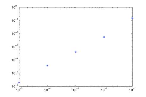
Figure 1: Discretization error for different time step

Figure 2 illustrates the dependence of the $L^{\infty}$ error on the space discretization parameter $n$. Here, we use a fixed time step-size $h=10^{-3}$ and compare the results with the result for $n=2^{14}+1$.

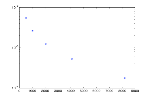
Figure 2: Discretization error for different space discretization

References

- [1] W. Bao and J. Shen, A fourth-order time-splitting Laguerre-Hermite pseudo-spectral method for Bose-Einstein condensates, SIAM J. Sci. Comput. 6 (2005), 2010–2028.
- [2] J. P. Borgna, A. Degasperis, M. De Leo, and D. Rial, Integrability of nonlinear wave equations and solvability of their initial value problem, J. Math. Phys. 53 (2012).
- [3] B. Bidegaray C. Besse and S. Descombes, Order estimates in the time of splitting methods for the nonlinear Schrödinger equation, SIAM J. Numer. Anal 40 (2002), 26–40.
- [4] T. Cazenave and A. Haraux, An introduction to semilinear evolutions equations, Oxford University Press, Clarendon, 1998.
- [5] S. Descombes and M. Thalhammer, The Lie-Trotter splitting method for nonlinear evolutionary problems involving critical parameters. An exact local error representation and application to nonlinear Schrödinger equations in the semi-classical regime, (2011), (in press).
- [6] B. Grébert E. Faou and E. Paturel, Birkhoff normal form for splitting methods applied to semilinear hamiltonian PDEs. Part ii: Abstract splitting, Numerische Mathematik 114 (2009), 459–490.
- [7] L. Gauckler, Convergence of a split-step Hermite method for the Gross-Pitaevskii equation, IMA J. Numer. Anal. 31 (2011), 396–415.
- [8] T. Jahnke and C. Lubich, Error bounds for exponential operator splitting, BIT40 4 (2000), 735–744.
- [9] M. De Leo and D. Rial, Well posedness and smoothing effect of Schrödinger-Poisson equation, J. Math. Phys. 48 (2007).
- [10] S. Masaki, Energy solution to a Schrödinger-Poisson system in the two-dimensional whole space, SIAM J. Math. Anal. 43 (2011), no. 6, 2719–2731.
- [11] J. Rauch, Nonlinear geometric optics, Department of Mathematics, University of Michigan (2000).
- [12] E. Tadmor, The exponential accuracy of Fourier and Chebyshev differencing methods, SIAM J. Numer. Anal. 23 (1986), no. 1, 1–10.
- [13] H. Yoshida, Construction of higher order symplectic integrators, Phys. Lett. A 150 (1990), 262–268.