The Monogenic Synchrosqueezed Wavelet Transform: A tool for the Decomposition/Demodulation of AM-FM images

M. Clausel, T. Oberlin, V. Perrier University of Grenoble and CNRS, Laboratoire Jean Kuntzmann UMR 5224, Saint Martin d’Hères, France.
Abstract

The synchrosqueezing method aims at decomposing 1D functions as superpositions of a small number of “Intrinsic Modes”, supposed to be well separated both in time and frequency. Based on the unidimensional wavelet transform and its reconstruction properties, the synchrosqueezing transform provides a powerful representation of multicomponent signals in the time-frequency plane, together with a reconstruction of each mode.

In this paper, a bidimensional version of the synchrosqueezing transform is defined, by considering a well–adapted extension of the concept of analytic signal to images: the monogenic signal. The natural bidimensional counterpart of the notion of Intrinsic Mode is then the concept of “Intrinsic Monogenic Mode” that we define. Thereafter, we investigate the properties of its associated Monogenic Wavelet Decomposition. This leads to a natural bivariate extension of the Synchrosqueezed Wavelet Transform, for decomposing and processing multicomponent images. Numerical tests validate the effectiveness of the method for different examples.

Keywords: monogenic signal, wavelet transform, directional time-frequency image analysis, synchrosqueezing.
MSC 2010: 65T60, 92C55, 94A08.

1 Introduction

In the past few years, there has been an increasing interest in representing images using spatially varying sinusoidal waves. As the understanding of the theory advanced, amplitude- and frequency-modulation (AM–FM) decompositions have been applied in a large range of problems: for example motion estimation using a flow–optical method based on an assumption of phase–invariance [1, 2, 3], reconstruction of breast cancer images [4, 5], texture analysis [6, 7], or ultrasound image segmentation methods [8] based on the concept of monogenic signal and quadrature filters [9]. A survey of applications of AM–FM decompositions in medical imaging can also be found in [10].

In each case, the main challenge is to decompose any input image s(x)𝑠𝑥s(x) into a sum of bidimensional AM–FM harmonics of the form

(1) s(x1,x2)==1Ls(t)==1LA(x1,x2)cos(φ(x1,x2)),𝑠subscript𝑥1subscript𝑥2superscriptsubscript1𝐿subscript𝑠𝑡superscriptsubscript1𝐿subscript𝐴subscript𝑥1subscript𝑥2subscript𝜑subscript𝑥1subscript𝑥2s(x_{1},x_{2})=\sum_{\ell=1}^{L}s_{\ell}(t)=\sum_{\ell=1}^{L}A_{\ell}(x_{1},x_{2})\cos(\varphi_{\ell}(x_{1},x_{2}))\;,

where A>0subscript𝐴0A_{\ell}>0 denotes a slowly–varying amplitude function, φsubscript𝜑\varphi_{\ell} denotes the phase, and =1,,L1𝐿\ell=1,\cdots,L indexes the different AM–FM harmonics. To each phase function, one can associate an instantaneous frequency vector field defined as ω=φsubscript𝜔subscript𝜑\omega_{\ell}=\nabla\varphi_{\ell}. Finding the components ssubscript𝑠s_{\ell} from the bidimensional signal s𝑠s is called the decomposition problem.

When the decomposition is given, another subsequent problem is to determine for each component ssubscript𝑠s_{\ell} its amplitude, phase and frequency functions involved in (1). The amplitudes can be related to the energy contained at each point of the image, whereas significant texture variations are captured in the frequency content. For example, in the case of a single component, the instantaneous frequency vectors are orthogonal to the isovalue intensity lines of an image, while their magnitudes provide a measure of local frequency content. The problem of estimating the amplitudes, phases and instantaneous frequencies of a signal of the form (1) (bidimensional or not) is called the demodulation problem.

In the one dimensional case, these two problems have been widely investigated both from the theoretical and practical point of view. To address the demodulation problem in the one dimensional setting, a first and necessary step is to define, in a proper way, the concept of amplitude, phase and instantaneous frequency of a given signal. To this end, one can use the well–known Hilbert transform, defined for any fL2()𝑓superscript𝐿2f\in L^{2}(\mathbb{R}) as

For a.e.t,f(t)=limε0(1π|ts|>εf(s)tsds).formulae-sequenceFor a.e.𝑡𝑓𝑡subscript𝜀01𝜋subscript𝑡𝑠𝜀𝑓𝑠𝑡𝑠differential-d𝑠\mbox{For a.e.}~{}t\in\mathbb{R},\,\mathcal{H}f(t)=\lim_{\varepsilon\to 0}\left(\frac{1}{\pi}\int_{|t-s|>\varepsilon}\frac{f(s)}{t-s}~{}\mathrm{d}s\right)\;.

The analytic signal associated to f𝑓f is then the complex–valued function F=(1+i)f𝐹1i𝑓F=(1+\mathrm{i}\mathcal{H})f. Thereafter, one defines amplitude A𝐴A and phase φ𝜑\varphi of f𝑓f as, respectively, the modulus and argument of the analytic signal F𝐹F associated to f𝑓f (the uniqueness of phase being ensured under smoothness assumptions on f𝑓f and under some initial conditions of the form φ(0)=φ0𝜑0subscript𝜑0\varphi(0)=\varphi_{0}). One then obtains

For a.e.t,F(t)=A(t)eiφ(t).formulae-sequenceFor a.e.𝑡𝐹𝑡𝐴𝑡superscriptei𝜑𝑡\mbox{For a.e.}~{}t\in\mathbb{R},\,F(t)=A(t)\mathrm{e}^{\mathrm{i}\varphi(t)}\;.

The instantaneous frequency of f𝑓f is thus the derivative of the phase φsuperscript𝜑\varphi^{\prime} [11]. The practical estimation of amplitude, phase and instantaneous frequency was the subject of numerous studies (see [12] for a survey). The “naive” method, which consists in using the Hilbert transform to estimate A𝐴A and φ𝜑\varphi, is known to be numerically unstable [13]. Alternative methods use the wavelet transform associated to reallocation techniques: in the one dimensional case, the time–frequency localization of wavelets allows to compute robust estimations of instantaneous frequency lines in the time-frequency representation: several approaches have been developed in the 90th, one should cite the method of “wavelet ridges” (see the two pioneer works [14] and [15]), the squeezing method introduced in [16] or the reassignment method [17].

On the other side, the decomposition problem consists in developing decompositions of any signal into a sum of “well–behaved” AM–FM components, and was widely studied. A recent attempt in this context is Empirical Mode Decomposition (EMD), initially introduced by Huang et al. in [18] and later popularized by Flandrin and his co–authors (see e.g. [19] or [20]).

Basically, EMD is the output of an iterative algorithm which provides an adaptive decomposition of any signal into several AM–FM components. It is now used in a wide range of applications including meteorology, structural stability analysis, and medical studies [12]. In spite of its simplicity and its efficiency, this method is hard to analyze mathematically, since it is defined in an empirical way. To tackle this problem, in [21], the authors propose and analyze an alternative method called “synchrosqueezing” derived from reassignment methods: they introduce a class of functions which can be viewed as the superposition of a reasonable number of modes, i.e. which read A(t)eiφ(t)subscriptsubscript𝐴𝑡superscripteisubscript𝜑𝑡\sum_{\ell}A_{\ell}(t)\mathrm{e}^{\mathrm{i}\varphi_{\ell}(t)}, where the amplitude A(t)subscript𝐴𝑡A_{\ell}(t) of each mode is slowly varying with respect to its instantaneous frequency ω(t)=φ(t)subscript𝜔𝑡superscriptsubscript𝜑𝑡\omega_{\ell}(t)=\varphi_{\ell}^{\prime}(t). For each function belonging to this class, the synchrosqueezing provides an estimation of this (unknown) decomposition. Synchrosqueezing presents many similarities with Empirical Mode Decomposition as shown in [21] (see also [22] for a comparison of these two methods or [23] for more about potential applications). In addition, since synchrosqueezing is based on the wavelet transform, it can be used to address simultaneously the decomposition and demodulation problem as done in [21].

In this paper, we will focus on the two dimensional case and extend the synchrosqueezing approach to images. Our first step consists in defining a convenient extension of the concept of analytic signal, in order to properly define the notion of amplitude and phase of an image. Two main generalizations of the analytic signal to the bidimensional setting have been considered in the literature: the hypercomplex and the monogenic signal defined respectively in [24] and [9]. Here, we focus on the monogenic setting, since its characteristics lead to easier interpretation. The monogenic signal associated to an image is defined using the Riesz transform. If we are given a real valued function fL2(2)𝑓superscript𝐿2superscript2f\in L^{2}(\mathbb{R}^{2}), one defines its Riesz transform f𝑓\mathcal{R}f as the following vector–valued function

f=(1f2f),𝑓matrixsubscript1𝑓subscript2𝑓\mathcal{R}f=\begin{pmatrix}\mathcal{R}_{1}f\\ \mathcal{R}_{2}f\end{pmatrix}\;,

where for any i=1,2𝑖12i=1,2 and a.e. x2𝑥superscript2x\in\mathbb{R}^{2} one has

if(x)=limε0(1π|xy|>ε(xiyi)|xy|3f(y)dy).subscript𝑖𝑓𝑥subscript𝜀01𝜋subscript𝑥𝑦𝜀subscript𝑥𝑖subscript𝑦𝑖superscript𝑥𝑦3𝑓𝑦differential-d𝑦\mathcal{R}_{i}f(x)=\lim_{\varepsilon\to 0}\left(\frac{1}{\pi}\int_{|x-y|>\varepsilon}\frac{(x_{i}-y_{i})}{|x-y|^{3}}f(y)~{}\mathrm{d}y\right)\;.

Then, the monogenic signal associated to f𝑓f is

f=(ff).𝑓matrix𝑓𝑓\mathcal{M}f=\begin{pmatrix}f\\ \mathcal{R}f\end{pmatrix}\;.

The characteristics of the monogenic signal are usually defined using the quaternionic formalism (see Appendix A for some background about quaternionic calculus and Appendix B for the main properties of the Riesz transform): the monogenic signal f𝑓\mathcal{M}f associated to f𝑓f can be read

f=f+1fi+2fj,𝑓𝑓subscript1𝑓isubscript2𝑓j\mathcal{M}f=f+\mathcal{R}_{1}f~{}\mathrm{i}+\mathcal{R}_{2}f~{}\mathrm{j}\;,

where (1,i,j,k)1ijk(1,\mathrm{i},\mathrm{j},\mathrm{k}) denotes the canonical basis of the algebra \mathbb{H} of the quaternions. In [9] and [25], it is proved that the monogenic signal can be written as

f=Aeφnθ=A(cosφ+nθsinφ) with nθ=cosθi+sinθj,𝑓𝐴superscripte𝜑subscript𝑛𝜃𝐴𝜑subscript𝑛𝜃𝜑 with subscript𝑛𝜃𝜃i𝜃j\mathcal{M}f=A~{}\mathrm{e}^{\varphi n_{\theta}}=A~{}(\cos\varphi+n_{\theta}\sin\varphi)\mbox{ with }n_{\theta}=\cos\theta~{}\mathrm{i}+\sin\theta~{}\mathrm{j}\;,

where A𝐴A is a positive real valued function and φ𝜑\varphi and θ𝜃\theta are two real valued functions defined in a unique way (under suitable assumptions). The function A𝐴A is called the amplitude of f𝑓f, φ𝜑\varphi its phase and nθsubscript𝑛𝜃n_{\theta} its local orientation. The function ω=φ𝜔𝜑\omega=\nabla\varphi will be called the instantaneous frequency of f𝑓f. To illustrate these definitions, we consider the case where f(x)=A0cos(kx)𝑓𝑥subscript𝐴0𝑘𝑥f(x)=A_{0}\cos(k\cdot x) with k=(k1,k2)𝑘subscript𝑘1subscript𝑘2k=(k_{1},k_{2}) and k1>0subscript𝑘10k_{1}>0. Set θ0=Arctan(k2/k1)subscript𝜃0Arctansubscript𝑘2subscript𝑘1\theta_{0}=\mathrm{Arctan}(k_{2}/k_{1}). One then has

f(x1,x2)=A0(sin(k1x1+k2x2)cosθ0sin(k1x1+k2x2)sinθ0)=A0k|k|sin(kx),𝑓subscript𝑥1subscript𝑥2subscript𝐴0matrixsubscript𝑘1subscript𝑥1subscript𝑘2subscript𝑥2subscript𝜃0subscript𝑘1subscript𝑥1subscript𝑘2subscript𝑥2subscript𝜃0subscript𝐴0𝑘𝑘𝑘𝑥\mathcal{R}f(x_{1},x_{2})=A_{0}\begin{pmatrix}\sin(k_{1}x_{1}+k_{2}x_{2})\cos\theta_{0}\\ \sin(k_{1}x_{1}+k_{2}x_{2})\sin\theta_{0}\end{pmatrix}=A_{0}\frac{k}{|k|}\sin(k\cdot x)\;,

and

f(x)=(f(x)f(x))=A0e(kx)(cosθ0i+sinθ0j).𝑓𝑥matrix𝑓𝑥𝑓𝑥subscript𝐴0superscripte𝑘𝑥subscript𝜃0isubscript𝜃0j\mathcal{M}f(x)=\begin{pmatrix}f(x)\\ \mathcal{R}f(x)\end{pmatrix}=A_{0}\mathrm{e}^{(k\cdot x)(\cos\theta_{0}~{}\mathrm{i}+\sin\theta_{0}~{}\mathrm{j})}\;.

Then for all x2𝑥superscript2x\in\mathbb{R}^{2}, one can set

A(x)=A0,φ(x)=kx,θ(x)=θ0=Arctan(k2/k1).formulae-sequence𝐴𝑥subscript𝐴0formulae-sequence𝜑𝑥𝑘𝑥𝜃𝑥subscript𝜃0Arctansubscript𝑘2subscript𝑘1A(x)=A_{0},\;\varphi(x)=k\cdot x,\;\theta(x)=\theta_{0}=\mathrm{Arctan}(k_{2}/k_{1})\;.

The aim of the present paper is to define the synchrosqueezing of bidimensional images, in the monogenic setting, in order to address both the decomposition and the demodulation problems. To this end, we will consider monogenic signals which are superposition of monogenic waves of the form

(2) A(x)eφ(x)nθ(x),𝐴𝑥superscripte𝜑𝑥subscript𝑛𝜃𝑥A(x)\mathrm{e}^{\varphi(x)n_{\theta(x)}}\;,

where A𝐴A and θ𝜃\theta are slowly varying functions with respect to φ𝜑\varphi.

We will consider successively the two different problems of deconvolution and decomposition. As in [21], our method is based on the continuous wavelet transform. Therefore, in Section 2, we recall a recent extension of the continuous bidimensional wavelet transform to the monogenic setting. We then investigate in Section 3, the problem of estimating the amplitude and instantaneous frequency of a monogenic spectral line of the form (2). Subsequently, we define in Section 4 the bidimensional synchrosqueezing and its application to the decomposition of multicomponent images. Finally, Section 5 gives some insights on the practical implementation of bidimensional synchrosqueezing, and provides numerical experiments. Proofs are postponed to Section 6 to make reading easier.

2 2D-wavelet transform and monogenic wavelet transform

In the one dimensional setting, the synchrosqueezing method is based on the one–dimensional wavelet analysis: indeed, the wavelet transform is used both to decompose an analytic signal into several components, and also to estimate the amplitude and the instantaneous frequency of each component. The main advantage of using the wavelet analysis is to avoid the use of the discrete Hilbert transform, since there is a link between the wavelet coefficients of the analytic signal associated to a real function f𝑓f, and its analytic wavelet coefficients (i.e. the wavelet coefficients of f𝑓f among an analytic wavelet).

In the bidimensional case, it is then quite natural to wonder if this approach can be extended using bidimensional wavelet analysis, replacing the analytic signal by the monogenic signal associated to our data. Since the monogenic signal can be viewed as a 3D vector field, it can be componentwise analyzed by the usual wavelet transform: Section 2.1 recalls first some basics about the bidimensional continuous wavelet transform. Thereafter in Section 2.2, we recall the main characteristics of the monogenic wavelet analysis, which is an extension of the usual wavelet analysis introduced in [26] and [27]. We would like to point out that, for any bidimensional real image f𝑓f, the wavelet coefficients of the monogenic signal f𝑓\mathcal{M}f can be related to the monogenic wavelet coefficients of f𝑓f (see Proposition 2.1 for a precise statement). Then, using monogenic wavelet analysis, one can recover the characteristics of the monogenic signal associated to our data, without estimating it.

In what follows, for any (a,b,α)+××(0,2π)𝑎𝑏𝛼subscriptsuperscript02𝜋(a,b,\alpha)\in\mathbb{R}^{*}_{+}\times\mathbb{R}\times(0,2\pi), we denote by Dasubscript𝐷𝑎D_{a} the dilation operator, Tbsubscript𝑇𝑏T_{b} the translation operator and Rαsubscript𝑅𝛼R_{\alpha} the rotation operator defined on L2(2)superscript𝐿2superscript2L^{2}(\mathbb{R}^{2}) by:

Daf(x)=a1f(x/a),Tbf(x)=f(xb),Rαf(x)=f(rα1x),formulae-sequencesubscript𝐷𝑎𝑓𝑥superscript𝑎1𝑓𝑥𝑎formulae-sequencesubscript𝑇𝑏𝑓𝑥𝑓𝑥𝑏subscript𝑅𝛼𝑓𝑥𝑓superscriptsubscript𝑟𝛼1𝑥D_{a}f(x)=a^{-1}f(x/a),\,T_{b}f(x)=f(x-b),\,R_{\alpha}f(x)=f(r_{\alpha}^{-1}x)\;,

where rαsubscript𝑟𝛼r_{\alpha} is the usual 2×2222\times 2 rotation matrix of angle α𝛼\alpha:

(3) rα=(cosαsinαsinαcosα).subscript𝑟𝛼matrix𝛼𝛼𝛼𝛼r_{\alpha}=\begin{pmatrix}\cos\alpha&-\sin\alpha\\ \sin\alpha&\cos\alpha\end{pmatrix}\;.

2.1 The usual bidimensional wavelet transform

We briefly recall classical definitions about the bidimensional continuous wavelet transform. A (real or complex) function ψL2(2)𝜓superscript𝐿2superscript2\psi\in L^{2}(\mathbb{R}^{2}) is called an admissible wavelet if it satisfies 111The Fourier Transform of ψ𝜓\psi being defined by: ψ^(ξ)=12π2ψ(x)eiξx𝑑x^𝜓𝜉12𝜋subscriptsuperscript2𝜓𝑥superscript𝑒𝑖𝜉𝑥differential-d𝑥\widehat{\psi}(\xi)=\frac{1}{2\pi}\int_{\mathbb{R}^{2}}\psi(x)e^{-i\xi\cdot x}dx :

(4) Cψ=(2π)22|ψ^(ξ)|2|ξ|2𝑑ξ<+subscript𝐶𝜓superscript2𝜋2subscriptsuperscript2superscript^𝜓𝜉2superscript𝜉2differential-d𝜉{C}_{\psi}=(2\pi)^{2}\int_{\mathbb{R}^{2}}\frac{|\widehat{\psi}(\xi)|^{2}}{|\xi|^{2}}~{}d\xi~{}<~{}+\infty

As usual (see [28]), the wavelet family {ψa,α,b}(a,α,b)+×(0,2π)×2subscriptsubscript𝜓𝑎𝛼𝑏𝑎𝛼𝑏subscriptsuperscript02𝜋superscript2\{\psi_{a,\alpha,b}\}_{(a,\alpha,b)\in\mathbb{R}^{*}_{+}\times(0,2\pi)\times\mathbb{R}^{2}} is defined by ψa,α,b=TbRαDaψsubscript𝜓𝑎𝛼𝑏subscript𝑇𝑏subscript𝑅𝛼subscript𝐷𝑎𝜓\psi_{a,\alpha,b}=T_{b}R_{\alpha}D_{a}\psi. One then defines the wavelet coefficients of any fL2(2)𝑓superscript𝐿2superscript2f\in L^{2}(\mathbb{R}^{2}) as follows:

cf(a,α,b)=2f(x)ψa,α,b(x)¯dx.subscript𝑐𝑓𝑎𝛼𝑏subscriptsuperscript2𝑓𝑥¯subscript𝜓𝑎𝛼𝑏𝑥differential-d𝑥c_{f}(a,\alpha,b)=\int_{\mathbb{R}^{2}}f(x)~{}\overline{\psi_{a,\alpha,b}(x)}~{}\mathrm{d}x\;.

If the wavelet is assumed to be isotropic, the wavelet coefficients do not depend on α𝛼\alpha. In this case, we will denote cf(a,b)=cf(a,0,b)subscript𝑐𝑓𝑎𝑏subscript𝑐𝑓𝑎0𝑏c_{f}(a,b)=c_{f}(a,0,b) and ψa,b=ψa,0,bsubscript𝜓𝑎𝑏subscript𝜓𝑎0𝑏\psi_{a,b}=\psi_{a,0,b}.

Any square integrable function f𝑓f can be recovered from its wavelet coefficients using the so–called reconstruction formula:

(5) f(x)=2πCψb2α(0,2π)a(0,+)cf(a,α,b)ψa,α,b(x)daa3dαdb,𝑓𝑥2𝜋subscript𝐶𝜓subscript𝑏superscript2subscript𝛼02𝜋subscript𝑎0subscript𝑐𝑓𝑎𝛼𝑏subscript𝜓𝑎𝛼𝑏𝑥d𝑎superscript𝑎3differential-d𝛼differential-d𝑏f(x)=\frac{2\pi}{C_{\psi}}\int_{b\in\mathbb{R}^{2}}\int_{\alpha\in(0,2\pi)}\int_{a\in(0,+\infty)}c_{f}(a,\alpha,b)~{}\psi_{a,\alpha,b}(x)~{}\frac{\mathrm{d}a}{a^{3}}\mathrm{d}\alpha~{}\mathrm{d}b\;,

where this equality stands in L2(2)superscript𝐿2superscript2L^{2}(\mathbb{R}^{2}). When the wavelet is assumed to be isotropic, we get a simpler expression:

f(x)=1Cψb2a(0,+)cf(a,b)ψa,b(x)daa3db.𝑓𝑥1subscript𝐶𝜓subscript𝑏superscript2subscript𝑎0subscript𝑐𝑓𝑎𝑏subscript𝜓𝑎𝑏𝑥d𝑎superscript𝑎3differential-d𝑏f(x)=\frac{1}{C_{\psi}}\int_{b\in\mathbb{R}^{2}}\int_{a\in(0,+\infty)}c_{f}(a,b)~{}\psi_{a,b}(x)~{}\frac{\mathrm{d}a}{a^{3}}\mathrm{d}b\;.

Other reconstruction formulas are available (see e.g. [28]), among which the pointwise reconstruction formula, obtained by summing over scales only. In the isotropic case, it reads:

(6) f(x)=2πC~ψ0+cf(a,x)daa2 with C~ψ=2ψ^(ξ)¯|ξ|2dξ.𝑓𝑥2𝜋subscript~𝐶𝜓superscriptsubscript0subscript𝑐𝑓𝑎𝑥d𝑎superscript𝑎2 with subscript~𝐶𝜓subscriptsuperscript2¯^𝜓𝜉superscript𝜉2differential-d𝜉\,f(x)=\frac{2\pi}{\tilde{C}_{\psi}}\int_{0}^{+\infty}c_{f}(a,x)~{}\frac{\mathrm{d}a}{a^{2}}\mbox{ with }\tilde{C}_{\psi}=\int_{\mathbb{R}^{2}}\frac{\overline{\widehat{\psi}(\xi)}}{|\xi|^{2}}~{}\mathrm{d}\xi\;.

As in the one dimensional case [21], this formula will play a special role in the bidimensional synchrosqueezing.
For any real function fL2(2)𝑓superscript𝐿2superscript2f\in L^{2}(\mathbb{R}^{2}), one can also define the wavelet transform of its monogenic signal F=f=f+1fi+2fj𝐹𝑓𝑓subscript1𝑓isubscript2𝑓jF=\mathcal{M}f=f+\mathcal{R}_{1}f~{}\mathrm{i}+\mathcal{R}_{2}f~{}\mathrm{j}\;, as:

cF=cf+c1fi+c2fj=(cfc1fc2f).subscript𝑐𝐹subscript𝑐𝑓subscript𝑐subscript1𝑓isubscript𝑐subscript2𝑓jmatrixsubscript𝑐𝑓subscript𝑐subscript1𝑓subscript𝑐subscript2𝑓c_{F}=c_{f}+c_{\mathcal{R}_{1}f}~{}\mathrm{i}+c_{\mathcal{R}_{2}f}~{}\mathrm{j}=\begin{pmatrix}c_{f}\\ c_{\mathcal{R}_{1}f}\\ c_{\mathcal{R}_{2}f}\end{pmatrix}\;.

2.2 The monogenic wavelet transform

We now present the continuous monogenic wavelet transform as defined in [26]. We consider a real admissible wavelet ψ𝜓\psi and define ψ(M)=ψ=(ψ1ψ2ψ)superscript𝜓𝑀𝜓matrix𝜓subscript1𝜓subscript2𝜓\psi^{(M)}=\mathcal{M}\psi=\begin{pmatrix}\psi\\ \mathcal{R}_{1}\psi\\ \mathcal{R}_{2}\psi\end{pmatrix} the associated monogenic wavelet. Observe that ψ(M)superscript𝜓𝑀\psi^{(M)} is also an admissible wavelet (taking values in 3superscript3\mathbb{R}^{3}), since each of its components satisfies relation (4). We define below the monogenic wavelet coefficients of a real function.

Definition 2.1

Let fL2(2)𝑓superscript𝐿2superscript2f\in L^{2}(\mathbb{R}^{2}). The monogenic wavelet coefficients cf(M)(a,α,b)superscriptsubscript𝑐𝑓𝑀𝑎𝛼𝑏c_{f}^{(M)}(a,\alpha,b) of f𝑓f are defined by:

(7) cf(M)(a,α,b)=2f(x)ψa,α,b(M)(x)dx,superscriptsubscript𝑐𝑓𝑀𝑎𝛼𝑏subscriptsuperscript2𝑓𝑥subscriptsuperscript𝜓𝑀𝑎𝛼𝑏𝑥differential-d𝑥c_{f}^{(M)}(a,\alpha,b)=\int_{\mathbb{R}^{2}}f(x)~{}{\psi^{(M)}_{a,\alpha,b}(x)}~{}\mathrm{d}x\;,

where for any (a,α,b)(0,+)×(0,2π)×2𝑎𝛼𝑏002𝜋superscript2(a,\alpha,b)\in(0,+\infty)\times(0,2\pi)\times\mathbb{R}^{2}, ψa,α,b(M)=TbRαDa(ψ)subscriptsuperscript𝜓𝑀𝑎𝛼𝑏subscript𝑇𝑏subscript𝑅𝛼subscript𝐷𝑎𝜓\psi^{(M)}_{a,\alpha,b}=T_{b}R_{\alpha}D_{a}(\mathcal{M}\psi).

Remark 2.1

For any (a,α,b)𝑎𝛼𝑏(a,\alpha,b), cf(M)(a,α,b)superscriptsubscript𝑐𝑓𝑀𝑎𝛼𝑏c_{f}^{(M)}(a,\alpha,b) is a Clifford vector, and thus can be written as cf(M)(a,α,b)=cf(a,α,b)+cf(1)(a,α,b)i+cf(2)(a,α,b)jsuperscriptsubscript𝑐𝑓𝑀𝑎𝛼𝑏subscript𝑐𝑓𝑎𝛼𝑏superscriptsubscript𝑐𝑓1𝑎𝛼𝑏isuperscriptsubscript𝑐𝑓2𝑎𝛼𝑏jc_{f}^{(M)}(a,\alpha,b)=c_{f}(a,\alpha,b)+c_{f}^{(1)}(a,\alpha,b)~{}\mathrm{i}+c_{f}^{(2)}(a,\alpha,b)~{}\mathrm{j} where we denote for i=1,2𝑖12i=1,2

cf(i)(a,α,b)=2f(x)(TbRαDaiψ)(x)dx,superscriptsubscript𝑐𝑓𝑖𝑎𝛼𝑏subscriptsuperscript2𝑓𝑥subscript𝑇𝑏subscript𝑅𝛼subscript𝐷𝑎subscript𝑖𝜓𝑥differential-d𝑥c_{f}^{(i)}(a,\alpha,b)=\int_{\mathbb{R}^{2}}f(x)~{}(T_{b}R_{\alpha}D_{a}\mathcal{R}_{i}\psi)(x)~{}\mathrm{d}x\;,

(see Appendix A for more details).

The next proposition states that there exists an explicit relationship between the monogenic coefficients of a real image f𝑓f and the usual wavelet coefficients of its monogenic signal f𝑓\mathcal{M}f.

Proposition 2.1

Let fL2(2)𝑓superscript𝐿2superscript2f\in L^{2}(\mathbb{R}^{2}) and denote by F=f𝐹𝑓F=\mathcal{M}f the monogenic signal associated to f𝑓f. Then for any (a,α,b)(0,+)×(0,2π)×2𝑎𝛼𝑏002𝜋superscript2(a,\alpha,b)\in(0,+\infty)\times(0,2\pi)\times\mathbb{R}^{2}

(8) cF(a,α,b)=(100rα)cf(M)(a,α,b).subscript𝑐𝐹𝑎𝛼𝑏matrix100subscript𝑟𝛼superscriptsubscript𝑐𝑓𝑀𝑎𝛼𝑏c_{F}(a,\alpha,b)=\begin{pmatrix}1&0\\ 0&-r_{\alpha}\end{pmatrix}c_{f}^{(M)}(a,\alpha,b)\;.

Proof.  We will prove that

cf(M)(a,α,b)=(100rα1)cF(a,α,b),superscriptsubscript𝑐𝑓𝑀𝑎𝛼𝑏matrix100superscriptsubscript𝑟𝛼1subscript𝑐𝐹𝑎𝛼𝑏c_{f}^{(M)}(a,\alpha,b)=\begin{pmatrix}1&0\\ 0&-r_{\alpha}^{-1}\end{pmatrix}c_{F}(a,\alpha,b)\;,

which is equivalent to (8). By definition of the monogenic wavelet transform one has:

cf(M)(a,α,b)=2f(x)TbRαDa(ψ)(x)dx.superscriptsubscript𝑐𝑓𝑀𝑎𝛼𝑏subscriptsuperscript2𝑓𝑥subscript𝑇𝑏subscript𝑅𝛼subscript𝐷𝑎𝜓𝑥differential-d𝑥c_{f}^{(M)}(a,\alpha,b)=\int_{\mathbb{R}^{2}}f(x)~{}{T_{b}R_{\alpha}D_{a}(\mathcal{M}\psi)}(x)~{}\mathrm{d}x\;.

The translation-, scale-invariance and steerability properties of the Riesz transform recalled in Propositions B.3 and B.4 of Appendix B, imply that:

TbRαDa(ψ)=rα1(ψa,α,b).subscript𝑇𝑏subscript𝑅𝛼subscript𝐷𝑎𝜓superscriptsubscript𝑟𝛼1subscript𝜓𝑎𝛼𝑏T_{b}R_{\alpha}D_{a}(\mathcal{R}\psi)=r_{\alpha}^{-1}\mathcal{R}(\psi_{a,\alpha,b})\;.

Hence

(9) 2f(x)TbRαDa(ψ)(x)dx=rα12f(x)(ψa,α,b)(x)dx.subscriptsuperscript2𝑓𝑥subscript𝑇𝑏subscript𝑅𝛼subscript𝐷𝑎𝜓𝑥differential-d𝑥superscriptsubscript𝑟𝛼1subscriptsuperscript2𝑓𝑥subscript𝜓𝑎𝛼𝑏𝑥differential-d𝑥\int_{\mathbb{R}^{2}}f(x)~{}{T_{b}R_{\alpha}D_{a}(\mathcal{R}\psi)}(x)~{}\mathrm{d}x=r_{\alpha}^{-1}\int_{\mathbb{R}^{2}}f(x)~{}{\mathcal{R}(\psi_{a,\alpha,b})(x)}~{}\mathrm{d}x\;.

Since by Proposition B.5, the Riesz transform is a componentwise antisymmetric operator on L2(2)superscript𝐿2superscript2L^{2}(\mathbb{R}^{2}), one deduces that:

(10) 2f(x)(ψa,α,b)(x)dx=(<f,1(ψa,α,b)>L2(2)<f,2(ψa,α,b)>L2(2))=2(f)(x)ψa,α,b(x)dx.\int_{\mathbb{R}^{2}}f(x){\mathcal{R}(\psi_{a,\alpha,b})(x)}~{}\mathrm{d}x=\begin{pmatrix}<f,\mathcal{R}_{1}(\psi_{a,\alpha,b})>_{L^{2}(\mathbb{R}^{2})}\\ <f,\mathcal{R}_{2}(\psi_{a,\alpha,b})>_{L^{2}(\mathbb{R}^{2})}\end{pmatrix}=-\int_{\mathbb{R}^{2}}(\mathcal{R}f)(x)~{}{\psi_{a,\alpha,b}(x)}~{}\mathrm{d}x\;.

Equations (9) and (10) then directly imply relation (8). \Box

We now consider the case an admissible isotropic real–valued wavelet ψ𝜓\psi. Examples include the Mexican hat (Laplacian of Gaussian) or the Morse wavelets (see [29] and Section 5). In such a case, the wavelets ψa,α,bsubscript𝜓𝑎𝛼𝑏\psi_{a,\alpha,b} as well as the wavelet coefficients cF(a,α,b)subscript𝑐𝐹𝑎𝛼𝑏c_{F}(a,\alpha,b) of the monogenic signal do not depend on the orientation α𝛼\alpha. From now, we then denote ψa,α,bsubscript𝜓𝑎𝛼𝑏\psi_{a,\alpha,b} and cF(a,α,b)subscript𝑐𝐹𝑎𝛼𝑏c_{F}(a,\alpha,b) respectively by ψa,bsubscript𝜓𝑎𝑏\psi_{a,b} and cF(a,b)subscript𝑐𝐹𝑎𝑏c_{F}(a,b). Thus equation (8) can be simplified in the following way:

(11) cF(a,b)=(100rα)cf(M)(a,α,b)=(100rα)(cf(a,b)cf(1)(a,α,b)cf(2)(a,α,b))=(cf(a,b)cosαcf(1)(a,α,b)+sinαcf(2)(a,α,b)sinαcf(1)(a,α,b)cosαcf(2)(a,α,b)).subscript𝑐𝐹𝑎𝑏matrix100subscript𝑟𝛼superscriptsubscript𝑐𝑓𝑀𝑎𝛼𝑏matrix100subscript𝑟𝛼matrixsubscript𝑐𝑓𝑎𝑏subscriptsuperscript𝑐1𝑓𝑎𝛼𝑏subscriptsuperscript𝑐2𝑓𝑎𝛼𝑏missing-subexpressionmatrixsubscript𝑐𝑓𝑎𝑏𝛼subscriptsuperscript𝑐1𝑓𝑎𝛼𝑏𝛼subscriptsuperscript𝑐2𝑓𝑎𝛼𝑏𝛼subscriptsuperscript𝑐1𝑓𝑎𝛼𝑏𝛼subscriptsuperscript𝑐2𝑓𝑎𝛼𝑏\begin{array}[]{lll}c_{F}(a,b)&=&\begin{pmatrix}1&0\\ 0&-r_{\alpha}\end{pmatrix}c_{f}^{(M)}(a,\alpha,b)=\begin{pmatrix}1&0\\ 0&-r_{\alpha}\end{pmatrix}\begin{pmatrix}c_{f}(a,b)\\ c^{(1)}_{f}(a,\alpha,b)\\ c^{(2)}_{f}(a,\alpha,b)\end{pmatrix}\\ &=&\begin{pmatrix}c_{f}(a,b)\\ -\cos\alpha~{}c^{(1)}_{f}(a,\alpha,b)+\sin\alpha~{}c^{(2)}_{f}(a,\alpha,b)\\ -\sin\alpha~{}c^{(1)}_{f}(a,\alpha,b)-\cos\alpha~{}c^{(2)}_{f}(a,\alpha,b)\end{pmatrix}\;.\end{array}

In practical situations, it will be easier to consider the case in which α=0𝛼0\alpha=0. We then get that

(12) cF(a,b)=(100Id)cf(M)(a,0,b).subscript𝑐𝐹𝑎𝑏matrix100𝐼𝑑superscriptsubscript𝑐𝑓𝑀𝑎0𝑏c_{F}(a,b)=\begin{pmatrix}1&0\\ 0&-Id\end{pmatrix}c_{f}^{(M)}(a,0,b)\;.

To sum up, in the isotropic case, the monogenic wavelet coefficients of the 2D real image f𝑓f can be related in a very simple way to the wavelet coefficients of the monogenic signal using (12). It will be useful in the sequel since when analyzing images, one deals with a real–valued signal f𝑓f and aims at recovering the wavelet coefficients cF(a,b)subscript𝑐𝐹𝑎𝑏c_{F}(a,b) of its monogenic signal F𝐹F without computing F𝐹F.

3 Wavelet analysis of bidimensional spectral lines

In this section, we tackle the problem of estimating the amplitude and instantaneous frequency of a bidimensional mode of the form A(x)eφ(x)n(x)𝐴𝑥superscripte𝜑𝑥𝑛𝑥A(x)\mathrm{e}^{\varphi(x)n(x)}. In the one dimensional setting, the “wavelet–ridge” method has proved to be efficient to address this problem [14, 15]. In [26, 29] it has been extended to the bidimensional setting using monogenic wavelet analysis.

Here we follow an alternative approach consisting in extending synchrosqueezing to the bidimensional context. We first define precisely the bidimensional modes that we are considering, and that we will call “Intrinsic Monogenic Mode Function” (IMMF). Then we deduce the notion of bidimensional frequency vector and state an approximation result using the monogenic wavelet transform.

Let us first define our concept of bidimensional modes:

Definition 3.1

Let ε>0𝜀0\varepsilon>0. An Intrinsic Monogenic Mode Function (IMMF) with accuracy ε𝜀\varepsilon and smoothness σ>0𝜎0\sigma>0 is a function FB˙,1σ(2,)𝐹subscriptsuperscript˙𝐵𝜎1superscript2F\in\dot{B}^{-\sigma}_{\infty,1}(\mathbb{R}^{2},\mathbb{H}) of the form

(13) F(x)=A(x)eφ(x)nθ(x) with nθ(x)=cos(θ(x))i+sin(θ(x))j,𝐹𝑥𝐴𝑥superscripte𝜑𝑥subscript𝑛𝜃𝑥 with subscript𝑛𝜃𝑥𝜃𝑥i𝜃𝑥jF(x)=A(x)\mathrm{e}^{\varphi(x)n_{\theta(x)}}\mbox{ with }n_{\theta(x)}=\cos(\theta(x))\mathrm{i}+\sin(\theta(x))\mathrm{j}\;,

where A>0𝐴0A>0 and A,θ𝒞1(2)L(2)𝐴𝜃superscript𝒞1superscript2superscript𝐿superscript2A,\theta\in\mathcal{C}^{1}(\mathbb{R}^{2})\cap L^{\infty}(\mathbb{R}^{2}), φ𝒞2(2)𝜑superscript𝒞2superscript2\varphi\in\mathcal{C}^{2}(\mathbb{R}^{2}). The function A𝐴A is called the amplitude of F𝐹F, whereas φ𝜑\varphi and nθsubscript𝑛𝜃n_{\theta} are called respectively the scalar phase and the local orientation of F𝐹F.
The function φ𝜑\varphi is assumed to have bounded derivatives of order 111 and 222:

(14) i{1,2}, 0<infx2|xiφ(x)|supx2|xiφ(x)|<.formulae-sequencefor-all𝑖12 0subscriptinfimum𝑥superscript2subscriptsubscript𝑥𝑖𝜑𝑥subscriptsupremum𝑥superscript2subscriptsubscript𝑥𝑖𝜑𝑥\forall i\in\{1,2\},\;0<\inf_{x\in\mathbb{R}^{2}}\left|\partial_{x_{i}}\varphi(x)\right|\leq\sup_{x\in\mathbb{R}^{2}}\left|\partial_{x_{i}}\varphi(x)\right|<\infty\;.
(15) M=maxi1,i2=1,2supx2|xi1xi22φ(x)|<.𝑀subscriptformulae-sequencesubscript𝑖1subscript𝑖212subscriptsupremum𝑥superscript2subscriptsuperscript2subscript𝑥subscript𝑖1subscript𝑥subscript𝑖2𝜑𝑥M=\max_{i_{1},i_{2}=1,2}\sup_{x\in\mathbb{R}^{2}}\left|\partial^{2}_{x_{i_{1}}x_{i_{2}}}\varphi(x)\right|<\infty\;.

Further we assume that A,θ,2φ𝐴𝜃superscript2𝜑A,\theta,\nabla^{2}\varphi are slowly varying functions with respect to φ𝜑\nabla\varphi, namely that for i=1,2𝑖12i=1,2

(16) x2,max(|xiA(x)|,|xiθ(x)|)ε|xiφ(x)|.formulae-sequencefor-all𝑥superscript2subscriptsubscript𝑥𝑖𝐴𝑥subscriptsubscript𝑥𝑖𝜃𝑥𝜀subscriptsubscript𝑥𝑖𝜑𝑥\forall x\in\mathbb{R}^{2},\max\left(|\partial_{x_{i}}A(x)|,|\partial_{x_{i}}\theta(x)|\right)\leq\varepsilon|\partial_{x_{i}}\varphi(x)|\;.

and

(17) x2,maxi1,i2=1,2|xi1xi22φ(x)|ε|φ(x)|.formulae-sequencefor-all𝑥superscript2subscriptformulae-sequencesubscript𝑖1subscript𝑖212subscriptsuperscript2subscript𝑥subscript𝑖1subscript𝑥subscript𝑖2𝜑𝑥𝜀𝜑𝑥\forall x\in\mathbb{R}^{2},\max_{i_{1},i_{2}=1,2}\left|\partial^{2}_{x_{i_{1}}x_{i_{2}}}\varphi(x)\right|\leq\varepsilon|\nabla\varphi(x)|\;.
Remark 3.1

Observe that, in the sequel, we shall consider non–square integrable functions. In this case, the two reconstruction formulas (5) and (6) may not hold (see Appendix B of [30]). We then need an additive assumption to ensure that the integral 0+cF(a,b)daa2superscriptsubscript0subscript𝑐𝐹𝑎𝑏d𝑎superscript𝑎2\int_{0}^{+\infty}c_{F}(a,b)\frac{\mathrm{d}a}{a^{2}}\; exists to give some sense to the reconstruction formula (6). Moreover, we will estimate the behavior of

a0+|cF(a,b)|daa2superscriptsubscriptsubscript𝑎0subscript𝑐𝐹𝑎𝑏d𝑎superscript𝑎2\int_{a_{0}}^{+\infty}|c_{F}(a,b)|\frac{\mathrm{d}a}{a^{2}}

for any a0>0subscript𝑎00a_{0}>0.
The additional hypothesis FB˙,1σ(2,)𝐹subscriptsuperscript˙𝐵𝜎1superscript2F\in\dot{B}^{-\sigma}_{\infty,1}(\mathbb{R}^{2},\mathbb{H}) for σ>0𝜎0\sigma>0 is equivalent to the following condition on the wavelet coefficients (see for e.g. [31]):

(18) FB˙,1σ=0supb2|cF(a,b)|daa2σ<+.subscriptnorm𝐹subscriptsuperscript˙𝐵𝜎1superscriptsubscript0subscriptsupremum𝑏superscript2subscript𝑐𝐹𝑎𝑏d𝑎superscript𝑎2𝜎\|F\|_{\dot{B}^{-\sigma}_{\infty,1}}=\int_{0}^{\infty}\sup_{b\in\mathbb{R}^{2}}|c_{F}(a,b)|\frac{\mathrm{d}a}{a^{2-\sigma}}<+\infty\;.

In such case, we easily deduce that for any a0>0subscript𝑎00a_{0}>0:

(19) supb2a0|cF(a,b)|daa2=supb2a0|cF(a,b)|1aσdaa2σa0σFB˙,1σsubscriptsupremum𝑏superscript2superscriptsubscriptsubscript𝑎0subscript𝑐𝐹𝑎𝑏d𝑎superscript𝑎2subscriptsupremum𝑏superscript2superscriptsubscriptsubscript𝑎0subscript𝑐𝐹𝑎𝑏1superscript𝑎𝜎d𝑎superscript𝑎2𝜎superscriptsubscript𝑎0𝜎subscriptnorm𝐹subscriptsuperscript˙𝐵𝜎1\sup_{b\in\mathbb{R}^{2}}\int_{a_{0}}^{\infty}|c_{F}(a,b)|\frac{\mathrm{d}a}{a^{2}}=\sup_{b\in\mathbb{R}^{2}}\int_{a_{0}}^{\infty}|c_{F}(a,b)|\frac{1}{a^{\sigma}}\frac{\mathrm{d}a}{a^{2-\sigma}}\leq a_{0}^{-\sigma}~{}\|F\|_{\dot{B}^{-\sigma}_{\infty,1}}

Moreover, by hypothesis, F𝒞1(2,)𝐹superscript𝒞1superscript2F\in\mathcal{C}^{1}(\mathbb{R}^{2},\mathbb{H}) and F𝐹\nabla F is bounded. Using the expression of the wavelet coefficients then implies that:

|cF(a,b)|a2FLxψL1,b2formulae-sequencesubscript𝑐𝐹𝑎𝑏superscript𝑎2subscriptnorm𝐹superscript𝐿subscriptnorm𝑥𝜓superscript𝐿1for-all𝑏superscript2|c_{F}(a,b)|\leq a^{2}\|\nabla F\|_{L^{\infty}}\|x\psi\|_{L^{1}}~{},~{}~{}~{}~{}\forall b\in\mathbb{R}^{2}

which ensures that for any a0>0subscript𝑎00a_{0}>0

(20) supb20a0|cF(a,b)|daa2<.subscriptsupremum𝑏superscript2superscriptsubscript0subscript𝑎0subscript𝑐𝐹𝑎𝑏d𝑎superscript𝑎2\sup_{b\in\mathbb{R}^{2}}\int_{0}^{a_{0}}|c_{F}(a,b)|\frac{\mathrm{d}a}{a^{2}}<\infty\;.

and finally leads to the existence of the integral 0+cF(a,b)daa2superscriptsubscript0subscript𝑐𝐹𝑎𝑏d𝑎superscript𝑎2\int_{0}^{+\infty}c_{F}(a,b)\frac{\mathrm{d}a}{a^{2}}.

Remark 3.2

In [29] authors considered spectral lines of the form f(x)=A(x)cos(φ(x))𝑓𝑥𝐴𝑥𝜑𝑥f(x)=A(x)\cos(\varphi(x)) with A,φ𝐴𝜑A,\nabla\varphi slowly varying with respect to φ𝜑\varphi. The authors then approximate the monogenic signal F𝐹F associated to f𝑓f by an IMMF of the form (13) with constant amplitude, linear phase and constant local orientation.

We now focus on the estimation of the amplitude and instantaneous frequency of an IMMF. To this end, we need some assumptions on the wavelet that we list below:
Assumptions (W)

  1. (i)

    the wavelet ψ𝜓\psi is isotropic and real–valued.

  2. (ii)

    ψW1,1(2)𝜓superscript𝑊11superscript2\psi\in W^{1,1}(\mathbb{R}^{2}).

  3. (iii)

    The first three moments of ψ𝜓\psi and ψ𝜓\nabla\psi are finite, namely

    supα{1,2,3}Iα<,supα{1,2,3}Iα<,formulae-sequencesubscriptsupremum𝛼123subscript𝐼𝛼subscriptsupremum𝛼123subscriptsuperscript𝐼𝛼\sup_{\alpha\in\{1,2,3\}}I_{\alpha}<\infty,\,\sup_{\alpha\in\{1,2,3\}}I^{\prime}_{\alpha}<\infty\;,

    where for any α>0𝛼0\alpha>0

    (21) Iα=2|x|α|ψ(x)|dx,Iα=2|x|α|ψ(x)|dx.formulae-sequencesubscript𝐼𝛼subscriptsuperscript2superscript𝑥𝛼𝜓𝑥differential-d𝑥subscriptsuperscript𝐼𝛼subscriptsuperscript2superscript𝑥𝛼𝜓𝑥differential-d𝑥I_{\alpha}=\int_{\mathbb{R}^{2}}|x|^{\alpha}|\psi(x)|\mathrm{d}x~{},~{}~{}\,I^{\prime}_{\alpha}=\int_{\mathbb{R}^{2}}|x|^{\alpha}|\nabla\psi(x)|\mathrm{d}x\;.

We first deal with the simple case of an IMMF of constant amplitude and phase:

Lemma 3.1

Let F𝐹F be an IMMF of the form F(x)=A0e(kx)nθ𝐹𝑥subscript𝐴0superscripte𝑘𝑥subscript𝑛𝜃F(x)=A_{0}\mathrm{e}^{(k\cdot x)n_{\theta}} with k=(k1,k2)2𝑘subscript𝑘1subscript𝑘2superscript2k=(k_{1},k_{2})\in\mathbb{R}^{2}, A0+,θformulae-sequencesubscript𝐴0subscriptsuperscript𝜃A_{0}\in\mathbb{R}^{*}_{+},\theta\in\mathbb{R}, and let ψ𝜓\psi be an isotropic real wavelet belonging to W1,1(2)superscript𝑊11superscript2W^{1,1}(\mathbb{R}^{2}).
The wavelet transform of F𝐹F is given by:

(22) cF(a,b)=A0aψ^(ak)(cos(kb)+sin(kb)(cosθi+sinθj))=aψ^(ak)(A0e(kb)nθ)subscript𝑐𝐹𝑎𝑏subscript𝐴0𝑎^𝜓𝑎𝑘𝑘𝑏𝑘𝑏𝜃i𝜃j𝑎^𝜓𝑎𝑘subscript𝐴0superscripte𝑘𝑏subscript𝑛𝜃c_{F}(a,b)=A_{0}a\widehat{\psi}(ak)\left(\cos(k\cdot b)+\sin(k\cdot b)(\cos\theta~{}\mathrm{i}+\sin\theta~{}\mathrm{j})\right)=a\widehat{\psi}(ak)\left(A_{0}\mathrm{e}^{(k\cdot b)n_{\theta}}\right)\,

and one has for i=1,2𝑖12i=1,2:

(23) bicF(a,b)=kinθ(aψ^(ak))(A0e(kb)nθ).subscriptsubscript𝑏𝑖subscript𝑐𝐹𝑎𝑏subscript𝑘𝑖subscript𝑛𝜃𝑎^𝜓𝑎𝑘subscript𝐴0superscripte𝑘𝑏subscript𝑛𝜃\partial_{b_{i}}c_{F}(a,b)=k_{i}n_{\theta}\left(a\widehat{\psi}(ak)\right)\left(A_{0}\mathrm{e}^{(k\cdot b)n_{\theta}}\right)\;.

The vectors k𝑘k and nθsubscript𝑛𝜃n_{\theta} can then be recovered using the two following relations:

k1nθ=b1cF(a,b)×(cF(a,b))1,subscript𝑘1subscript𝑛𝜃subscriptsubscript𝑏1subscript𝑐𝐹𝑎𝑏superscriptsubscript𝑐𝐹𝑎𝑏1k_{1}n_{\theta}=\partial_{b_{1}}c_{F}(a,b)\times(c_{F}(a,b))^{-1}\;,
k2nθ=b2cF(a,b)×(cF(a,b))1.subscript𝑘2subscript𝑛𝜃subscriptsubscript𝑏2subscript𝑐𝐹𝑎𝑏superscriptsubscript𝑐𝐹𝑎𝑏1k_{2}n_{\theta}=\partial_{b_{2}}c_{F}(a,b)\times(c_{F}(a,b))^{-1}\;.

Proof.  By definition, since the wavelet is isotropic real, one has:

cF(a,b)=a12F(x)ψ(xba)dx=a2F(au+b)ψ(u)dusubscript𝑐𝐹𝑎𝑏superscript𝑎1subscriptsuperscript2𝐹𝑥𝜓𝑥𝑏𝑎differential-d𝑥𝑎subscriptsuperscript2𝐹𝑎𝑢𝑏𝜓𝑢differential-d𝑢c_{F}(a,b)=a^{-1}\int_{\mathbb{R}^{2}}F(x)\psi\left(\frac{x-b}{a}\right)\mathrm{d}x=a\int_{\mathbb{R}^{2}}F(au+b)\psi(u)\mathrm{d}u

A simple calculation leads to:

cF(a,b)=aA0(2cos(k(au+b))ψ(u)ducosθ2sin(k(au+b))ψ(u)dusinθ2sin(k(au+b))ψ(u)du)=A0aψ^(ak)(cos(k.b)sin(k.b)cos(θ)sin(k.b)sin(θ))=aψ^(ak)F(b).c_{F}(a,b)=aA_{0}\begin{pmatrix}\int_{\mathbb{R}^{2}}\cos(k\cdot(au+b))\psi(u)\mathrm{d}u\\ \cos\theta\int_{\mathbb{R}^{2}}\sin(k\cdot(au+b))\psi(u)\mathrm{d}u\\ \sin\theta\int_{\mathbb{R}^{2}}\sin(k\cdot(au+b))\psi(u)\mathrm{d}u\end{pmatrix}=A_{0}a\widehat{\psi}(ak)\begin{pmatrix}\cos(k.b)\\ \sin(k.b)\cos(\theta)\\ \sin(k.b)\sin(\theta)\end{pmatrix}=a\widehat{\psi}(ak)F(b)\;.

where we have used ψ^(ak)=ψ^(ak)^𝜓𝑎𝑘^𝜓𝑎𝑘\widehat{\psi}(-ak)=\widehat{\psi}(ak) since the wavelet is isotropic.

Now, since ψW1,1(2)𝜓superscript𝑊11superscript2\psi\in W^{1,1}(\mathbb{R}^{2}) and FL(2)𝐹superscript𝐿superscript2F\in L^{\infty}(\mathbb{R}^{2}), we get:

bicF(a,b)=a12F(x)bi[ψ(xba)]dx=a22F(x)(xiψ)(xba)dx.subscriptsubscript𝑏𝑖subscript𝑐𝐹𝑎𝑏superscript𝑎1subscriptsuperscript2𝐹𝑥subscriptsubscript𝑏𝑖delimited-[]𝜓𝑥𝑏𝑎d𝑥superscript𝑎2subscriptsuperscript2𝐹𝑥subscriptsubscript𝑥𝑖𝜓𝑥𝑏𝑎differential-d𝑥\partial_{b_{i}}c_{F}(a,b)=a^{-1}\int_{\mathbb{R}^{2}}F(x)\partial_{b_{i}}\left[\psi\left(\frac{x-b}{a}\right)\right]\mathrm{d}x=-a^{-2}\int_{\mathbb{R}^{2}}F(x)(\partial_{x_{i}}\psi)\left(\frac{x-b}{a}\right)\mathrm{d}x\;.

A similar calculation, using xiψ^(ξ)=iξiψ^(ξ),ξ=(ξ1,ξ2)formulae-sequence^subscriptsubscript𝑥𝑖𝜓𝜉isubscript𝜉i^𝜓𝜉for-all𝜉subscript𝜉1subscript𝜉2\widehat{\partial_{x_{i}}\psi}(\xi)=\rm i\xi_{i}\widehat{\psi}(\xi),\forall\xi=(\xi_{1},\xi_{2}), and ψ𝜓\psi isotropic, yields:

bicF(a,b)=A0akiψ^(ak)(sin(k.b)cos(k.b)cos(θ)cos(k.b)sin(θ))=akiψ^(ak)nθF(b),\partial_{b_{i}}c_{F}(a,b)=A_{0}ak_{i}\widehat{\psi}(ak)\begin{pmatrix}-\sin(k.b)\\ \cos(k.b)\cos(\theta)\\ \cos(k.b)\sin(\theta)\end{pmatrix}=ak_{i}\widehat{\psi}(ak)~{}n_{\theta}F(b)\;,

where we have used:

nθF(b)=nθ(cos(kb)+nθsin(kb))=sin(kb)+nθcos(kb).subscript𝑛𝜃𝐹𝑏subscript𝑛𝜃𝑘𝑏subscript𝑛𝜃𝑘𝑏𝑘𝑏subscript𝑛𝜃𝑘𝑏n_{\theta}F(b)=n_{\theta}(\cos(k\cdot b)+n_{\theta}\sin(k\cdot b))=-\sin(k\cdot b)+n_{\theta}\cos(k\cdot b).

This leads to (23). \Box

Remark that, more generally, if F(x)=A0e(kx+α)nθ𝐹𝑥subscript𝐴0superscripte𝑘𝑥𝛼subscript𝑛𝜃F(x)=A_{0}\mathrm{e}^{(k\cdot x+\alpha)n_{\theta}}, (α𝛼\alpha\in\mathbb{R}):

(24) cF(a,b)subscript𝑐𝐹𝑎𝑏\displaystyle c_{F}(a,b) =\displaystyle= A0aψ^(ak)e(kb+α)nθ=aψ^(ak)F(b)subscript𝐴0𝑎^𝜓𝑎𝑘superscripte𝑘𝑏𝛼subscript𝑛𝜃𝑎^𝜓𝑎𝑘𝐹𝑏\displaystyle A_{0}a\widehat{\psi}(ak)\mathrm{e}^{(k\cdot b+\alpha)n_{\theta}}=a\widehat{\psi}(ak)~{}F(b)
(25) bicF(a,b)subscriptsubscript𝑏𝑖subscript𝑐𝐹𝑎𝑏\displaystyle\partial_{b_{i}}c_{F}(a,b) =\displaystyle= akiψ^(ak)nθF(b)𝑎subscript𝑘𝑖^𝜓𝑎𝑘subscript𝑛𝜃𝐹𝑏\displaystyle ak_{i}\widehat{\psi}(ak)~{}n_{\theta}F(b)

The formulas (22) and (23) can be extended in the general case of an IMMF F𝐹F of the form (13).

Proposition 3.1

Let ψ𝜓\psi a wavelet satisfying assumptions (W) and F𝐹F an IMMF with accuracy ε𝜀\varepsilon and smoothness σ>0𝜎0\sigma>0 of the form (13). For all (a,b)+×2𝑎𝑏subscriptsuperscriptsuperscript2(a,b)\in\mathbb{R}^{*}_{+}\times\mathbb{R}^{2}, one has

  1. (i)
    cF(a,b)=aψ^(aφ(b))(A(b)eφ(b)n(b))+εa2R1(a,b),subscript𝑐𝐹𝑎𝑏𝑎^𝜓𝑎𝜑𝑏𝐴𝑏superscripte𝜑𝑏𝑛𝑏𝜀superscript𝑎2subscript𝑅1𝑎𝑏c_{F}(a,b)=a\widehat{\psi}(a\nabla\varphi(b))\left(A(b)\mathrm{e}^{\varphi(b)n(b)}\right)+\varepsilon a^{2}R_{1}(a,b)\;,

    with

    (26) |R1(a,b)|I1(2A(b)+1)|φ(b)|+aI2A(b)(|φ(b)|+2M)/2+aI2M/2+a2I3A(b)M/6.subscript𝑅1𝑎𝑏subscript𝐼12𝐴𝑏1𝜑𝑏𝑎subscript𝐼2𝐴𝑏𝜑𝑏2𝑀2missing-subexpressionmissing-subexpression𝑎subscript𝐼2𝑀2superscript𝑎2subscript𝐼3𝐴𝑏𝑀6\begin{array}[]{lll}|R_{1}(a,b)|&\leq&I_{1}(\sqrt{2}A(b)+1)|\nabla\varphi(b)|+aI_{2}A(b)\left(\left|\nabla\varphi(b)\right|+\sqrt{2}M\right)/2\\ &&+aI_{2}M/2+a^{2}I_{3}A(b)M/6\;.\end{array}
  2. (ii)
    bicF(a,b)=biφ(b)nθ(b)(aψ^(aφ(b)))(A(b)eφ(b)nθ(b))+εaR2(a,b),subscriptsubscript𝑏𝑖subscript𝑐𝐹𝑎𝑏subscriptsubscript𝑏𝑖𝜑𝑏subscript𝑛𝜃𝑏𝑎^𝜓𝑎𝜑𝑏𝐴𝑏superscripte𝜑𝑏subscript𝑛𝜃𝑏𝜀𝑎subscript𝑅2𝑎𝑏\partial_{b_{i}}c_{F}(a,b)=\partial_{b_{i}}\varphi(b)n_{\theta(b)}\left(a\widehat{\psi}(a\nabla\varphi(b))\right)\left(A(b)\mathrm{e}^{\varphi(b)n_{\theta(b)}}\right)+\varepsilon aR_{2}(a,b)\;,

    with

    (27) |R2(a,b)|A(b)(a|φ(b)|I2/2+a2MI3/6)+(2A(b)+1)(|φ(b)|I1+aMI2/2).subscript𝑅2𝑎𝑏𝐴𝑏𝑎𝜑𝑏subscriptsuperscript𝐼22superscript𝑎2𝑀subscriptsuperscript𝐼36missing-subexpressionmissing-subexpression2𝐴𝑏1𝜑𝑏subscriptsuperscript𝐼1𝑎𝑀subscriptsuperscript𝐼22\begin{array}[]{lll}|R_{2}(a,b)|&\leq&A(b)\left(a\left|\nabla\varphi(b)\right|I^{\prime}_{2}/2+a^{2}MI^{\prime}_{3}/6\right)\\ &&+\left(\sqrt{2}A(b)+1\right)\left(|\nabla\varphi(b)|I^{\prime}_{1}+aMI^{\prime}_{2}/2\right)\;.\end{array}
Remark 3.3

As a consequence of this proposition, since in the isotropic case cF(a,b)subscript𝑐𝐹𝑎𝑏c_{F}(a,b) and cf(M)(a,α,b)superscriptsubscript𝑐𝑓𝑀𝑎𝛼𝑏c_{f}^{(M)}(a,\alpha,b) are related by (11), the above proposition specifies the results stated in [26] and [29]. Notably, it gives a bound of the approximation error.

Proof.  See Section 6.1. \Box

We now define the two following Clifford vectors:

(28) Λ1(a,b)subscriptΛ1𝑎𝑏\displaystyle\Lambda_{1}(a,b) =\displaystyle= b1cF(a,b)×(cF(a,b))1,subscriptsubscript𝑏1subscript𝑐𝐹𝑎𝑏superscriptsubscript𝑐𝐹𝑎𝑏1\displaystyle~{}\partial_{b_{1}}c_{F}(a,b)\times(c_{F}(a,b))^{-1}\;,
Λ2(a,b)subscriptΛ2𝑎𝑏\displaystyle\Lambda_{2}(a,b) =\displaystyle= b2cF(a,b)×(cF(a,b))1.subscriptsubscript𝑏2subscript𝑐𝐹𝑎𝑏superscriptsubscript𝑐𝐹𝑎𝑏1\displaystyle~{}\partial_{b_{2}}c_{F}(a,b)\times(c_{F}(a,b))^{-1}\;.

These two vectors will provide an approximation of the vectors biφ(b)nθ(b)subscriptsubscript𝑏𝑖𝜑𝑏subscript𝑛𝜃𝑏\partial_{b_{i}}\varphi(b)n_{\theta(b)} for an IMMF F𝐹F of the form (13). More precisely, we can state the following result:

Theorem 3.2

Let F𝐹F be an IMMF with accuracy ε>0𝜀0\varepsilon>0 and smoothness σ>0𝜎0\sigma>0 of the form (13). Assume that we are given ψ𝜓\psi a wavelet satisfying assumptions (W) and consider (a,b)+×2𝑎𝑏subscriptsuperscriptsuperscript2(a,b)\in\mathbb{R}^{*}_{+}\times\mathbb{R}^{2} such that

|cF(a,b)|εν for some ν(0,1/2).subscript𝑐𝐹𝑎𝑏superscript𝜀𝜈 for some 𝜈012|c_{F}(a,b)|\geq\varepsilon^{\nu}\mbox{ for some }\nu\in(0,1/2)\;.

Then for i=1,2𝑖12i=1,2:

(29) |Λi(a,b)biφ(b)nθ(b)|ε1νa(|R2(a,b)|+a|R1(a,b)||φ(b)|)subscriptΛ𝑖𝑎𝑏subscriptsubscript𝑏𝑖𝜑𝑏subscript𝑛𝜃𝑏superscript𝜀1𝜈𝑎subscript𝑅2𝑎𝑏𝑎subscript𝑅1𝑎𝑏𝜑𝑏|\Lambda_{i}(a,b)-\partial_{b_{i}}\varphi(b)n_{\theta(b)}|\leq\varepsilon^{1-\nu}a~{}\left(|R_{2}(a,b)|+a|R_{1}(a,b)|~{}|\nabla\varphi(b)|\right)

where R1subscript𝑅1R_{1}, R2subscript𝑅2R_{2} have been defined respectively in (26) and (27). In addition for any a0>0subscript𝑎00a_{0}>0, there exists some ε0>0subscript𝜀00\varepsilon_{0}>0 such that, for all (a,b)(0,a0)×2𝑎𝑏0subscript𝑎0superscript2(a,b)\in(0,a_{0})\times\mathbb{R}^{2} and any 0<εε00𝜀subscript𝜀00<\varepsilon\leq\varepsilon_{0}:

(30) |Λi(a,b)biφ(b)nθ(b)|ενsubscriptΛ𝑖𝑎𝑏subscriptsubscript𝑏𝑖𝜑𝑏subscript𝑛𝜃𝑏superscript𝜀𝜈|\Lambda_{i}(a,b)-\partial_{b_{i}}\varphi(b)n_{\theta(b)}|\leq\varepsilon^{\nu}

Proof.  See Section 6.2. \Box

Since cos(φ(x))=cos(φ(x))𝜑𝑥𝜑𝑥\cos(\varphi(x))=\cos(-\varphi(x)), there is an ambiguity in the definition of the instantaneous frequency φ𝜑\nabla\varphi since φ𝜑\varphi can be replaced by φ𝜑-\varphi. To solve this problem, practitioners usually assume that the first component of the instantaneous frequency is positive (see [10] and references therein for more details). Under this additional assumption, our method yields an estimate of the amplitude and of the instantaneous frequency of an IMMF:

Proposition 3.3

The notations and assumptions are those of Theorem 3.2. In addition, we assume that:

x2,x1φ(x)>0.formulae-sequencefor-all𝑥superscript2subscriptsubscript𝑥1𝜑𝑥0\forall x\in\mathbb{R}^{2},\,\partial_{x_{1}}\varphi(x)>0\;.

Then for i=1,2𝑖12i=1,2, and (a,b)(0,a0)×𝑎𝑏0subscript𝑎0(a,b)\in(0,a_{0})\times\mathbb{R}:

(31) |b1φ(b)|Λ1(a,b)||εν.subscriptsubscript𝑏1𝜑𝑏subscriptΛ1𝑎𝑏superscript𝜀𝜈|\partial_{b_{1}}\varphi(b)-|\Lambda_{1}(a,b)||\leq\varepsilon^{\nu}\;.

and

(32) |b2φ(b)|Λ2(a,b)|sgn(Re(b1cF(a,b)b2cF(a,b)¯))|εν.limit-fromsubscriptsubscript𝑏2𝜑𝑏subscriptΛ2𝑎𝑏sgnResubscriptsubscript𝑏1subscript𝑐𝐹𝑎𝑏¯subscriptsubscript𝑏2subscript𝑐𝐹𝑎𝑏superscript𝜀𝜈|\partial_{b_{2}}\varphi(b)-|\Lambda_{2}(a,b)|~{}\mathrm{sgn}(\mathrm{Re}(\partial_{b_{1}}c_{F}(a,b)~{}\overline{\partial_{b_{2}}c_{F}(a,b)}))|\leq\varepsilon^{\nu}\;.

Proof.  See Section 6.3. \Box

4 Decomposition of a multi–component image into spectral lines

In this section we will consider a more general context, where our model is now a superposition of several IMMFs (introduced in Section 3), assumed to be well separated, as defined in the following definition 4.1. We will show in Theorem 4.1 how such functions can be decomposed into monogenic modes, using synchrosqueezing. Thereafter, for each component, the associated amplitude and instantaneous frequency will be estimated using the results of Section 3.

Definition 4.1

A function F𝐹F defined from 2superscript2\mathbb{R}^{2} to \mathbb{H} is said to be a superposition of well separated Intrinsic Monogenic Mode Components with smoothness σ>0𝜎0\sigma>0 up to accuracy ε>0𝜀0\varepsilon>0 and with separation d>0𝑑0d>0, if there exists a finite integer L𝐿L such that

(33) F(x)==1LF(x),𝐹𝑥superscriptsubscript1𝐿subscript𝐹𝑥F(x)=\sum_{\ell=1}^{L}F_{\ell}(x)\;,

where all the Fsubscript𝐹F_{\ell} are IMMFs with accuracy ε𝜀\varepsilon and smoothness σσ>0subscript𝜎𝜎0\sigma_{\ell}\geq\sigma>0 of the form (13): F(x)=A(x)eφ(x)nθ(x)subscript𝐹𝑥subscript𝐴𝑥superscriptesubscript𝜑𝑥subscript𝑛subscript𝜃𝑥F_{\ell}(x)=A_{\ell}(x)~{}\mathrm{e}^{\varphi_{\ell}(x)n_{\theta_{\ell}(x)}}, and moreover satisfy for any x𝑥x, >superscript\ell>\ell^{\prime} and i{1,2}𝑖12i\in\{1,2\}:

(34) |xiφ(x)|>|xiφ(x)|,subscriptsubscript𝑥𝑖subscript𝜑𝑥subscriptsubscript𝑥𝑖subscript𝜑superscript𝑥\left|\partial_{x_{i}}\varphi_{\ell}(x)\right|>\left|\partial_{x_{i}}\varphi_{\ell^{\prime}}(x)\right|\;,

and

(35) |xiφ(x)nθ(x)xiφ(x)nθ(x)|d[|xiφ(x)|+|xiφ(x)|].subscriptsubscript𝑥𝑖subscript𝜑𝑥subscript𝑛subscript𝜃𝑥subscriptsubscript𝑥𝑖subscript𝜑superscript𝑥subscript𝑛subscript𝜃superscript𝑥𝑑delimited-[]subscriptsubscript𝑥𝑖subscript𝜑𝑥subscriptsubscript𝑥𝑖subscript𝜑superscript𝑥\left|\partial_{x_{i}}\varphi_{\ell}(x)n_{\theta_{\ell}(x)}-\partial_{x_{i}}\varphi_{\ell^{\prime}}(x)n_{\theta_{\ell^{\prime}}(x)}\right|\geq d~{}\left[\left|\partial_{x_{i}}\varphi_{\ell}(x)\right|+\left|\partial_{x_{i}}\varphi_{\ell^{\prime}}(x)\right|\right]\;.

We denote by 𝒜ε,σ,dsubscript𝒜𝜀𝜎𝑑\mathcal{A}_{\varepsilon,\sigma,d} the class of all functions F𝐹F satisfying these conditions.

We now define the monogenic synchrosqueezing transform (MSST) of a function F𝐹F belonging to 𝒜ε,σ,dsubscript𝒜𝜀𝜎𝑑\mathcal{A}_{\varepsilon,\sigma,d}.

Definition 4.2

Assume that we are given ψ𝜓\psi a wavelet satisfying assumptions (W) such that

supp(ψ^){ξ2;1Δ|ξ|1+Δ},supp^𝜓formulae-sequence𝜉superscript21Δ𝜉1Δ\mathrm{supp}(\widehat{\psi})\subset\{\xi\in\mathbb{R}^{2}~{};~{}1-\Delta\leq|\xi|\leq 1+\Delta\}\;,

with

(36) Δ<d2(1+d).Δ𝑑21𝑑\Delta<\frac{d}{2(1+d)}\;.

Consider h𝒞c(,)subscriptsuperscript𝒞𝑐h\in\mathcal{C}^{\infty}_{c}(\mathbb{R},\mathbb{R}) such that h(x)dx=1subscript𝑥differential-d𝑥1\int_{\mathbb{R}}h(x)\mathrm{d}x=1. Let δ>0𝛿0\delta>0, ν(0,1)𝜈01\nu\in(0,1), and ε>0𝜀0\varepsilon>0. For F𝒜ε,σ,d𝐹subscript𝒜𝜀𝜎𝑑F\in\mathcal{A}_{\varepsilon,\sigma,d}, the monogenic synchrosqueezing transform of F𝐹F is defined for any (b,k,n)2×2×𝕊1𝑏𝑘𝑛superscript2superscript2superscript𝕊1(b,k,n)\in\mathbb{R}^{2}\times\mathbb{R}^{2}\times\mathbb{S}^{1} (𝕊1superscript𝕊1\mathbb{S}^{1} being the unit sphere of 2superscript2\mathbb{R}^{2}) by

(37) SF,εδ,ν(b,k,n)=Aε,F(b)cF(a,b)1δ2h(k1Re(n¯Λ1(a,b))δ)h(k2Re(n¯Λ2(a,b))δ)daa2,superscriptsubscript𝑆𝐹𝜀𝛿𝜈𝑏𝑘𝑛subscriptsubscript𝐴𝜀𝐹𝑏subscript𝑐𝐹𝑎𝑏1superscript𝛿2subscript𝑘1Re¯𝑛subscriptΛ1𝑎𝑏𝛿subscript𝑘2Re¯𝑛subscriptΛ2𝑎𝑏𝛿d𝑎superscript𝑎2S_{F,\varepsilon}^{\delta,\nu}(b,k,n)=\int_{A_{\varepsilon,F}(b)}c_{F}(a,b)\frac{1}{\delta^{2}}h\left(\frac{k_{1}-{\rm Re}(\overline{n}~{}\Lambda_{1}(a,b))}{\delta}\right)h\left(\frac{k_{2}-{\rm Re}(\overline{n}~{}\Lambda_{2}(a,b))}{\delta}\right)\frac{\mathrm{d}a}{a^{2}}\;,

with

Aε,F(b)={a+;|cF(a,b)|>εν},subscript𝐴𝜀𝐹𝑏formulae-sequence𝑎subscriptsubscript𝑐𝐹𝑎𝑏superscript𝜀𝜈A_{\varepsilon,F}(b)=\{a\in\mathbb{R}_{+}~{};\,|c_{F}(a,b)|>\varepsilon^{\nu}\}\;,

and where Λ1(a,b)subscriptΛ1𝑎𝑏\Lambda_{1}(a,b), Λ2(a,b)subscriptΛ2𝑎𝑏\Lambda_{2}(a,b) are defined by equation (28).

We can now state our main result:

Theorem 4.1

The notations are those of Definition 4.2. Let F𝒜ε,σ,d𝐹subscript𝒜𝜀𝜎𝑑F\in\mathcal{A}_{\varepsilon,\sigma,d} and ν(0,1/(2+4/σ))𝜈0124𝜎\nu\in(0,1/(2+4/\sigma)). Provided that ε>0𝜀0\varepsilon>0 is sufficiently small, the following assertions hold:

  • |cF(a,b)|>ενsubscript𝑐𝐹𝑎𝑏superscript𝜀𝜈|c_{F}(a,b)|>\varepsilon^{\nu} only if there exists some \ell such that

    (38) (a,b)Z={(a,b),|a|φ(b)|1|<Δ}.𝑎𝑏subscript𝑍𝑎𝑏𝑎subscript𝜑𝑏1Δ(a,b)\in Z_{\ell}=\left\{(a,b),\,\left|a|\nabla\varphi_{\ell}(b)|-1\right|<\Delta\right\}\;.
  • For each ={1,,L}1𝐿\ell=\{1,\cdots,L\} and each pair (a,b)Z𝑎𝑏subscript𝑍(a,b)\in Z_{\ell} for which |cF(a,b)|>ενsubscript𝑐𝐹𝑎𝑏superscript𝜀𝜈|c_{F}(a,b)|>\varepsilon^{\nu}, one has for i=1,2𝑖12i=1,2 and for some C>0𝐶0C>0:

    |Λi(a,b)iφ(b)nθ(b)|Cεν.subscriptΛ𝑖𝑎𝑏subscript𝑖subscript𝜑𝑏subscript𝑛subscript𝜃𝑏𝐶superscript𝜀𝜈|\Lambda_{i}(a,b)-\partial_{i}\varphi_{\ell}(b)n_{\theta_{\ell}(b)}|\leq C\varepsilon^{\nu}\;.
  • Moreover for any {1,,L}1𝐿\ell\in\{1,\cdots,L\}, there exists C>0𝐶0C>0, such that for any b2𝑏superscript2b\in\mathbb{R}^{2}

    limδ0|12πC~ψ𝕊1(εν,n,b)Sf,εδ(b,k,n)dkdnA(b)eφ(b)nθ(b)|Cεν.subscript𝛿012𝜋subscript~𝐶𝜓subscriptsuperscript𝕊1subscriptsubscriptsuperscript𝜀𝜈𝑛𝑏subscriptsuperscript𝑆𝛿𝑓𝜀𝑏𝑘𝑛differential-d𝑘differential-d𝑛subscript𝐴𝑏superscriptesubscript𝜑𝑏subscript𝑛subscript𝜃𝑏𝐶superscript𝜀𝜈\lim_{\delta\rightarrow 0}\left|\frac{1}{2\pi\tilde{C}_{\psi}}\int_{\mathbb{S}^{1}}\int_{{\cal B}_{\ell}(\varepsilon^{\nu},n,b)}S^{\delta}_{f,\varepsilon}(b,k,n)\mathrm{d}k\mathrm{d}n-A_{\ell}(b)\mathrm{e}^{\varphi_{\ell}(b)n_{\theta_{\ell}(b)}}\right|\leq C\varepsilon^{\nu}\;.

    where we denote (εν,n,b)={k2;maxi|kinbiφ(b)nθ(b)|εν}subscriptsuperscript𝜀𝜈𝑛𝑏formulae-sequence𝑘superscript2subscript𝑖subscript𝑘𝑖𝑛subscriptsubscript𝑏𝑖subscript𝜑𝑏subscript𝑛subscript𝜃𝑏superscript𝜀𝜈{\cal B}_{\ell}(\varepsilon^{\nu},n,b)=\{k\in\mathbb{R}^{2}~{};\,\max_{i}|k_{i}n-\partial_{b_{i}}\varphi_{\ell}(b)n_{\theta_{\ell}(b)}|\leq\varepsilon^{\nu}\}, and where C~ψsubscript~𝐶𝜓\tilde{C}_{\psi} was introduced in (6).

Proof.  See Section 6.4. \Box

5 Implementation and numerical experiments

This section aims to illustrate the efficiency of the monogenic synchrosqueezing transform, and its potential applications. We will first describe the computation of the discrete MSST from a N×N𝑁𝑁N\times N discrete image, then we will show some examples on artificial and real images.

5.1 The discrete monogenic synchrosqueezing transform

The first step consists in the discretization of the variables, therefore one builds discrete sets 𝒜𝒜\mathcal{A}, 𝒦𝒦\mathcal{K}, 𝒪𝒪\mathcal{O} for the scales a𝑎a, the normalized frequencies (k1,k2)subscript𝑘1subscript𝑘2(k_{1},k_{2}), and the orientations θ𝜃\theta respectively, the frequency resolution in k𝑘k being denoted by ΔksubscriptΔ𝑘\Delta_{k}. Note that one usually chooses a logarithmic scale for a𝑎a and k𝑘k, e.g. 𝒜={2j/nv}j=0na1,𝒜subscriptsuperscript2𝑗subscript𝑛𝑣𝑗0subscript𝑛𝑎1\mathcal{A}=\{2^{j/n_{v}}\}_{j=0\cdots n_{a}-1}, so that we have nvsubscript𝑛𝑣n_{v} coefficients per octave. Then, we compute the discrete monogenic wavelet transform cF(a,b)subscript𝑐𝐹𝑎𝑏c_{F}(a,b), and the estimations of the instantaneous frequencies Λ1(a,b)subscriptΛ1𝑎𝑏\Lambda_{1}(a,b) and Λ2(a,b)subscriptΛ2𝑎𝑏\Lambda_{2}(a,b) defined in equation (28) by writing for i=1,2𝑖12i=1,2:

bicf(a,b)=2f(x)biψa,b(x)dx,subscriptsubscript𝑏𝑖subscript𝑐𝑓𝑎𝑏subscriptsuperscript2𝑓𝑥subscriptsubscript𝑏𝑖subscript𝜓𝑎𝑏𝑥d𝑥\partial_{b_{i}}c_{f}(a,b)=\int_{\mathbb{R}^{2}}f(x)\partial_{b_{i}}\psi_{a,b}(x)~{}\mathrm{d}x,

the other components bic1f(a,b)subscriptsubscript𝑏𝑖subscript𝑐subscript1𝑓𝑎𝑏\partial_{b_{i}}c_{\mathcal{R}_{1}f}(a,b) and bic2f(a,b)subscriptsubscript𝑏𝑖subscript𝑐subscript2𝑓𝑎𝑏\partial_{b_{i}}c_{\mathcal{R}_{2}f}(a,b) being computed in the same manner. The monogenic synchrosqueezing transform consists in a partial reallocation of the monogenic wavelet transform according to space, frequency and orientation parameters. Given a threshold γ𝛾\gamma, and for all a𝒜,(k1,k2)𝒦2,θ𝒪formulae-sequence𝑎𝒜formulae-sequencesubscript𝑘1subscript𝑘2superscript𝒦2𝜃𝒪a\in\mathcal{A},(k_{1},k_{2})\in\mathcal{K}^{2},\theta\in\mathcal{O}, one simply writes

(39) SF,γ(b,k1,k2,nθ)=log(2)nva𝒜 s.t. {|cF(a,b)|>γ|k1Re(Λ1(a,b)n¯θ)|Δk12|k2Re(Λ2(a,b)n¯θ)|Δk22cF(a,b)a.subscript𝑆𝐹𝛾𝑏subscript𝑘1subscript𝑘2subscript𝑛𝜃2subscript𝑛𝑣subscript𝑎𝒜 s.t. casessubscript𝑐𝐹𝑎𝑏𝛾subscript𝑘1ResubscriptΛ1𝑎𝑏subscript¯𝑛𝜃subscriptΔsubscript𝑘12subscript𝑘2ResubscriptΛ2𝑎𝑏subscript¯𝑛𝜃subscriptΔsubscript𝑘22subscript𝑐𝐹𝑎𝑏𝑎S_{F,\gamma}(b,k_{1},k_{2},n_{\theta})=\frac{\log(2)}{n_{v}}\sum_{a\in\mathcal{A}\mbox{ s.t. }\left\{\begin{array}[]{l}|c_{F}(a,b)|>\gamma\\ \left|k_{1}-{\rm Re}(\Lambda_{1}(a,b)~{}\overline{n}_{\theta})\right|\leq\frac{\Delta_{k_{1}}}{2}\\ \left|k_{2}-{\rm Re}(\Lambda_{2}(a,b)~{}\overline{n}_{\theta})\right|\leq\frac{\Delta_{k_{2}}}{2}\end{array}\right.}\frac{c_{F}(a,b)}{a}.

The term log(2)anv2𝑎subscript𝑛𝑣\frac{\log(2)}{an_{v}} comes from the measure daa2𝑑𝑎superscript𝑎2\frac{da}{a^{2}} in equation (37), as we deal with logarithmic scales. Note that if we use a logarithmic scale for the frequencies like in [21], the resolution ΔksubscriptΔ𝑘\Delta_{k} depends on the value k𝑘k.

This discrete MSST is relatively easy and cheap to compute, but it is not of great interest in practice because of the large number of variables which prevents both easy representation and fast processing (i.e. decomposition, demodulation). To decrease this number of variables, one can remark that if a superposition of IMMFs satisfies the separation condition of equation (34), then for any >superscript\ell>\ell^{\prime} it also satisfies |φ(x)|>|φ(x)|,subscript𝜑𝑥subscript𝜑superscript𝑥|\nabla\varphi_{\ell}(x)|>|\nabla\varphi_{\ell^{\prime}}(x)|, so that the IMMFs are also separated in terms of the norm of the frequency vector. This leads us to define the following discrete isotropic MSST for all a𝒜𝑎𝒜a\in\mathcal{A} and k𝒦𝑘𝒦k\in\mathcal{K}:

(40) SF,γ(b,k)=log(2)nva𝒜 s.t. {|cF(a,b)|>γ|k|Λ1(a,b)|2+|Λ2(a,b)|2|Δk2cF(a,b)a.subscript𝑆𝐹𝛾𝑏𝑘2subscript𝑛𝑣subscript𝑎𝒜 s.t. casessubscript𝑐𝐹𝑎𝑏𝛾𝑘superscriptsubscriptΛ1𝑎𝑏2superscriptsubscriptΛ2𝑎𝑏2subscriptΔ𝑘2subscript𝑐𝐹𝑎𝑏𝑎S_{F,\gamma}(b,k)=\frac{\log(2)}{n_{v}}\sum_{a\in\mathcal{A}\mbox{ s.t. }\left\{\begin{array}[]{l}|c_{F}(a,b)|>\gamma\\ \left|k-\sqrt{|\Lambda_{1}(a,b)|^{2}+|\Lambda_{2}(a,b)|^{2}}\right|\leq\frac{\Delta_{k}}{2}\\ \end{array}\right.}\frac{c_{F}(a,b)}{a}.

Intuitively, SF,γ(b,kp)subscript𝑆𝐹𝛾𝑏subscript𝑘𝑝S_{F,\gamma}(b,k_{p}) contains all the coefficients cF(a,b)subscript𝑐𝐹𝑎𝑏c_{F}(a,b) whose “instantaneous isotropic frequency“ |Λ1(a,b)|2+|Λ2(a,b)|2superscriptsubscriptΛ1𝑎𝑏2superscriptsubscriptΛ2𝑎𝑏2\sqrt{|\Lambda_{1}(a,b)|^{2}+|\Lambda_{2}(a,b)|^{2}} is around the value k𝑘k. The latter isotropic MSST can be particularly useful when visualizing the time-frequency distribution, as it only depends on three scalar parameters (b1,b2,k)subscript𝑏1subscript𝑏2𝑘(b_{1},b_{2},k), that is by far easier to represent. Hence, this version will be used in the experiments hereafter. Additionally we will use the Morlet wavelet with parameters μ>0𝜇0\mu>0 and σ>0𝜎0\sigma>0, defined in the Fourier domain as follows

(41) ψ^μ,σ(ξ)=exp(π2σ(|ξ|μ)2).subscript^𝜓𝜇𝜎𝜉superscript𝜋2𝜎superscript𝜉𝜇2\hat{\psi}_{\mu,\sigma}(\xi)=\exp(-\pi^{2}\sigma(|\xi|-\mu)^{2})\;.

5.2 Representing a synthetic 3-components signal

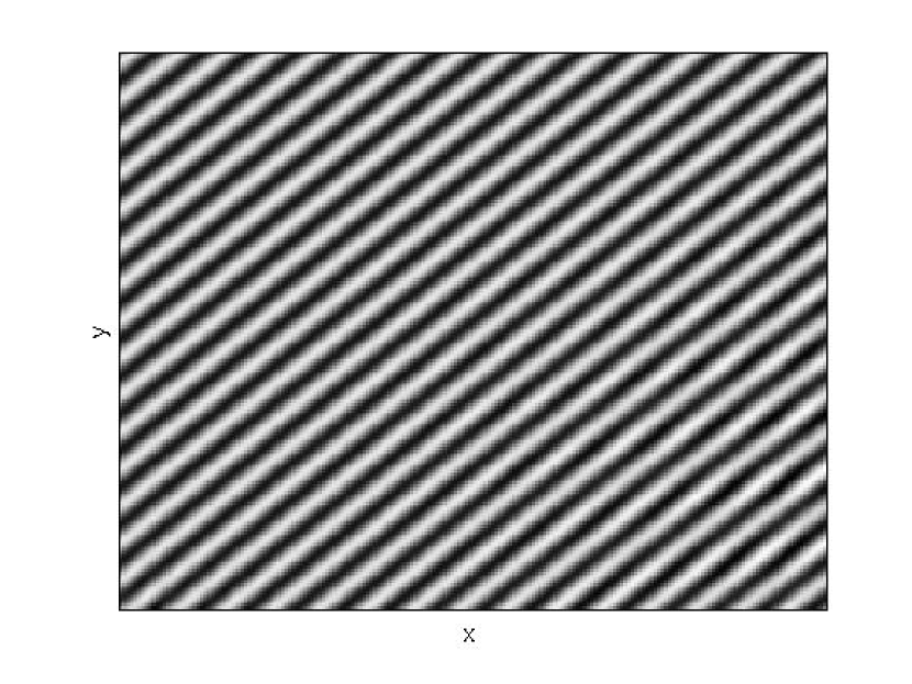
This section illustrates the interest in using the MSST to represent multicomponent signals in 2 dimensions. Let us first define the synthetic 3-components test-signal f=f1+f2+f3𝑓subscript𝑓1subscript𝑓2subscript𝑓3f=f_{1}+f_{2}+f_{3} with

(42) {f1(x,y)=e10((x0.5)2+(y0.5).2))sin(10π(x2+y2+2(x+0.2y))f2(x,y)=1.2sin(40π(x+y))f3(x,y)=cos(2π(70x+20x2+50y20y241xy))\left\{\begin{array}[]{lll}f_{1}(x,y)&=&e^{-10((x-0.5)^{2}+(y-0.5).^{2}))}\sin(10\pi(x^{2}+y^{2}+2(x+0.2y))\\ f_{2}(x,y)&=&1.2\sin(40\pi(x+y))\\ f_{3}(x,y)&=&\cos(2\pi(70x+20x^{2}+50y-20y^{2}-41xy))\end{array}\right.

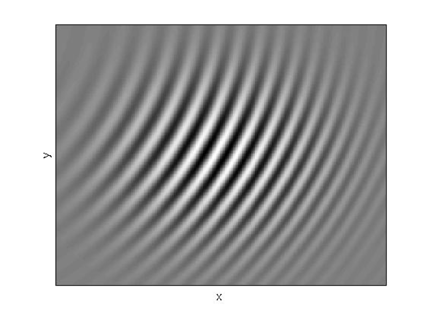
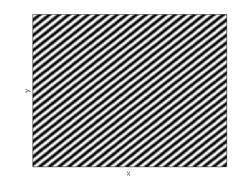
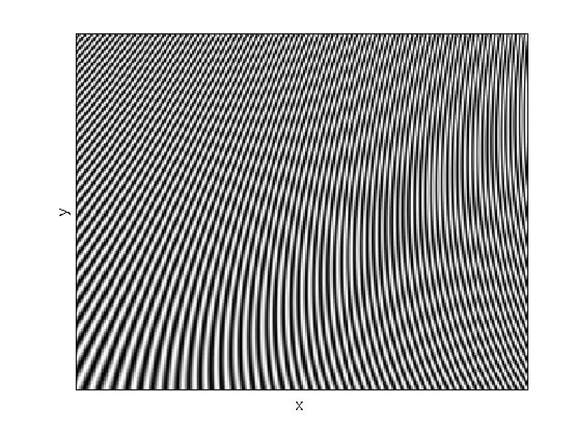
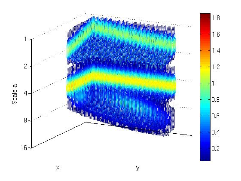
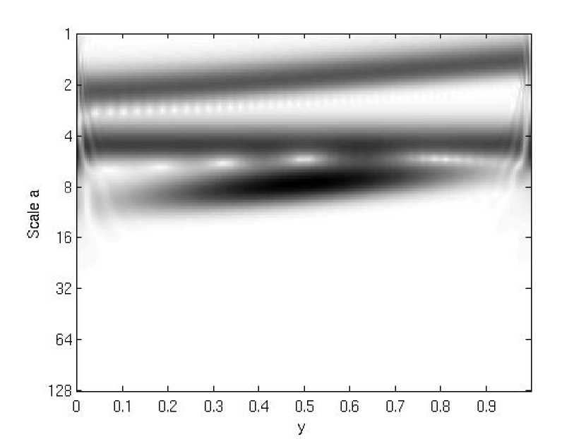
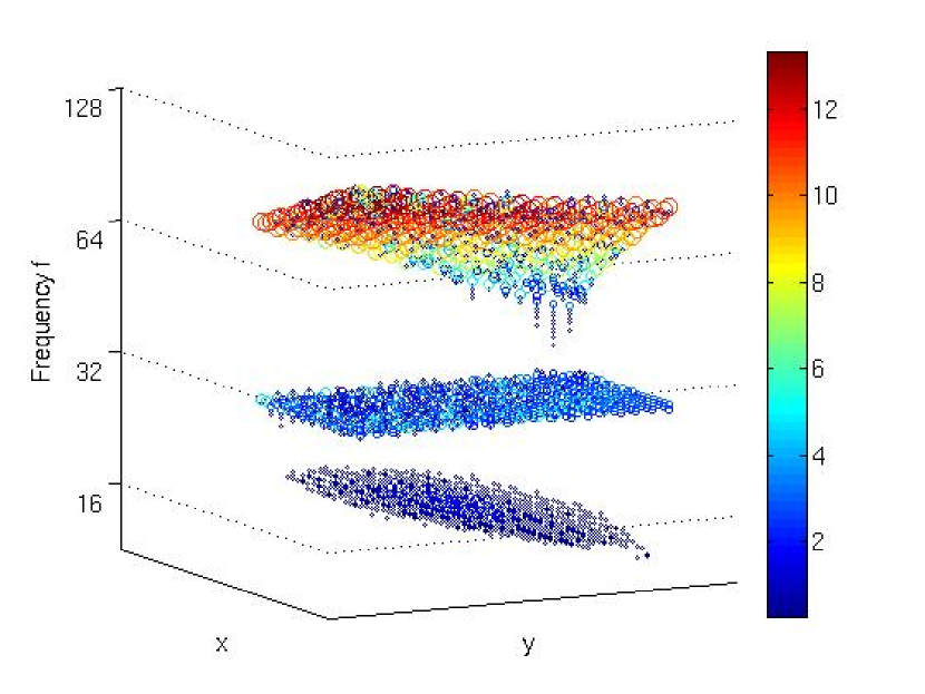
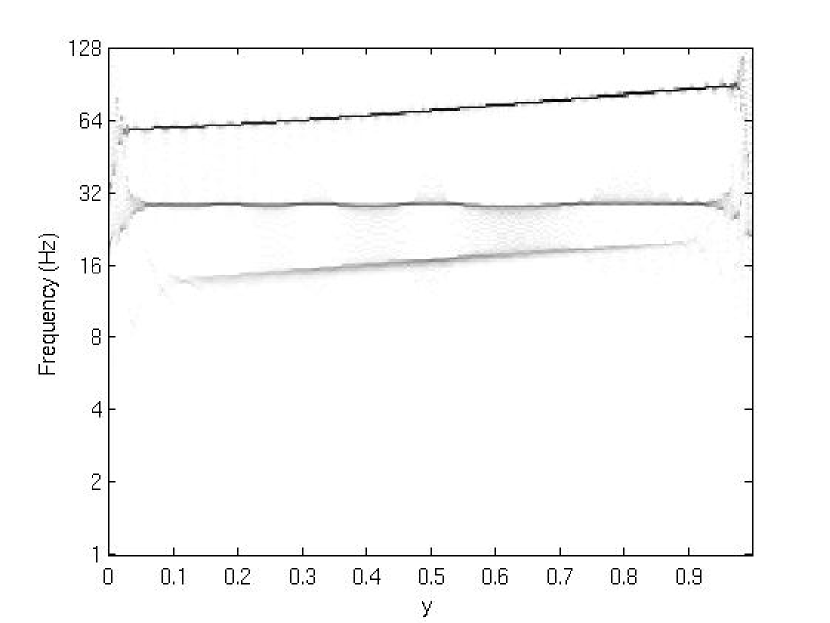
We compute both its monogenic isotropic wavelet transform cFsubscript𝑐𝐹c_{F} and its isotropic MSST SFsubscript𝑆𝐹S_{F}. We then aim at representing |cF|subscript𝑐𝐹|c_{F}| (resp. |SF|subscript𝑆𝐹|S_{F}|), which depends on the three scalar parameters x𝑥x, y𝑦y and a𝑎a (resp. k𝑘k). We will here propose two distinct visualizations: either a 3-dimensional scatter “density” plot, or a 2-dimensional representation for x𝑥x or y𝑦y fixed, which looks similar to a 1D continuous wavelet representation. The following Figure 1 shows these different representations for the wavelet and the MSST of the signal (42). We see how the MSST sharpens the time-scale representation, making it more readable.

Refer to caption

(a)

Refer to caption

(b)

Refer to caption

(c)

Refer to caption

(d)

Refer to caption

(e)

Refer to caption

(f)

Refer to caption

(g)

Refer to caption

(h)

Figure 1: (a): the 2D test-signal represented as an image. (b,c,d): its components. (e,f): the monogenic wavelet transform |cF|subscript𝑐𝐹|c_{F}| represented as a density in 3D, and in 2D for y=0.5𝑦0.5y=0.5 fixed. (g,h): the same visualizations of the MSST |SF|subscript𝑆𝐹|S_{F}|.

5.3 Decomposition and Demodulation

Once the MSST has been computed, the key point to separate and reconstruct the modes is to identify the instantaneous (anisotropic) frequency of each mode |φ(b)|subscript𝜑𝑏|\nabla\varphi_{\ell}(b)| at each point b𝑏b. The thsuperscript𝑡\ell^{th} IMMF Fsubscript𝐹F_{\ell} is then approximated by F^(b)subscript^𝐹𝑏\widehat{F}_{\ell}(b) as follows:

(43) F^(b)=k^(b)κkk^(b)+κSF,γ(b,k).subscript^𝐹𝑏subscriptsubscript^𝑘𝑏𝜅𝑘subscript^𝑘𝑏𝜅subscript𝑆𝐹𝛾𝑏𝑘\widehat{F}_{\ell}(b)=\sum_{\hat{k}_{\ell}(b)-\kappa\leq k\leq\hat{k}_{\ell}(b)+\kappa}S_{F,\gamma}(b,k)\;.

where k^(b)subscript^𝑘𝑏\hat{k}_{\ell}(b) is an appropriate estimate of |φ(b)|subscript𝜑𝑏|\nabla\varphi_{\ell}(b)|. Obtaining this estimate is an involved problem which will not be discussed here, so we simply use the approach used in  [21] based on a greedy algorithm. Our approximation F^(b)subscript^𝐹𝑏\widehat{F}_{\ell}(b) of the thsuperscript𝑡\ell^{th} IMMF is computed by summing the coefficients of the synchrosqueezed transform in the vicinity of this instantaneous frequency, to regularize the solution. In practice the width κ𝜅\kappa of the window is set to 5Δk5subscriptΔ𝑘5\Delta_{k}. To evaluate the method, we compare the mode Fsubscript𝐹F_{\ell} of the test-signal defined in equation (42) to the corresponding mode F^subscript^𝐹\hat{F}_{\ell} obtained from the discrete MSST after extraction, by computing the normalized Mean-Squared Error (MSE):

(44) MSE(F^)=F^FF.𝑀𝑆𝐸subscript^𝐹delimited-∥∥subscript^𝐹subscript𝐹delimited-∥∥subscript𝐹MSE(\hat{F}_{\ell})=\frac{\lVert\hat{F}_{\ell}-F_{\ell}\rVert}{\lVert F_{\ell}\rVert}\;.

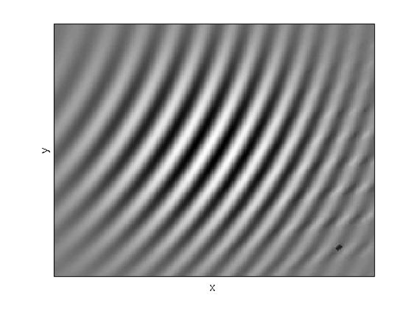
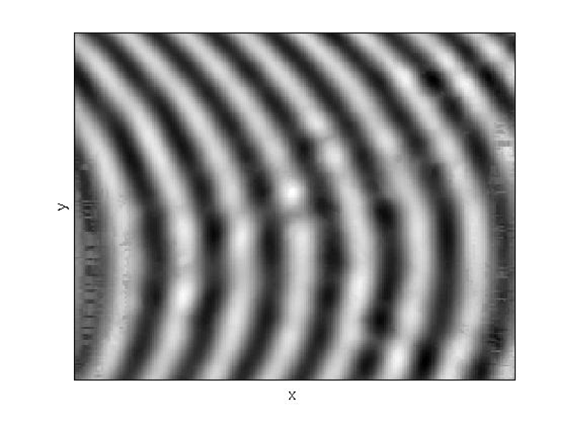
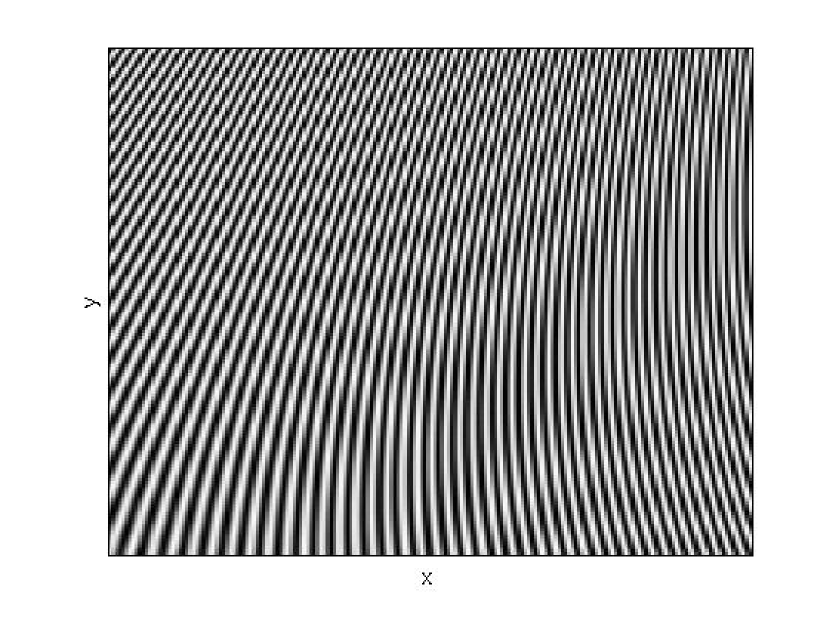
Each reconstructed IMMF is displayed on Figure 2, where one also provides the corresponding MSE. It is clear that the modes are reconstructed with very high accuracy, although our method for ridge extraction is quite simple.
Refer to caption

(a)

Refer to caption

(b)

Refer to caption

(c)

Figure 2: The extracted and reconstructed modes 1, 2 and 3 for the test signal of equation (42). The normalized MSE are respectively 0.030.030.03, 0.060.060.06 and 0.050.050.05. We used the Morlet Wavelet ψμ,σsubscript𝜓𝜇𝜎\psi_{\mu,\sigma} defined in (41) with σ=2𝜎2\sigma=2 and μ=1𝜇1\mu=1, and removed the border (1818\frac{1}{8} at each side for each dimension) to avoid border effects.

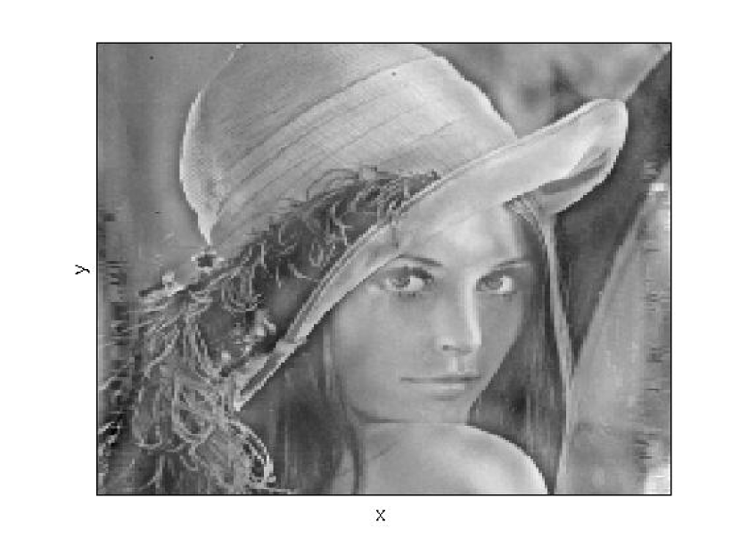
Finally, we aim here at showing that the MSST remains efficient on real images or textures, even though they can not be considered as multicomponent signals. The following example shows the image Lenna where we artificially added an oscillating pattern. After a 2D synchrosqueezing transform one is able to extract the oscillating component to roughly reconstruct the original image. Note that this kind of image was first introduced in [27] to illustrate the discrete monogenic wavelet transform.
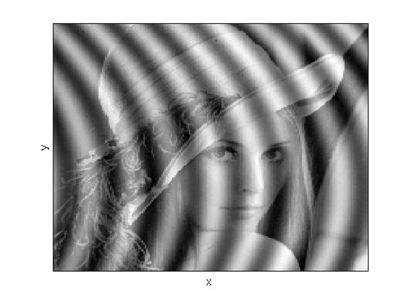
Refer to caption

(a)

Refer to caption

(b)

Refer to caption

(c)

Figure 3: Illustration of possible applications on real images. (a): Input image, Lenna plus an oscillating pattern. (b): the extracted mode by the 2D MSST. The parameters are the same as for Figure 2. The MSE is 0.12. (c): The residual approximates the original Lenna image.

6 Proofs

6.1 Proof of Proposition 3.1

We prove Proposition 3.1 into several steps.

6.1.1 A preliminary result

We first need a preliminary result:

Lemma 6.1

Assume that F𝐹F is an IMMF with accuracy ε𝜀\varepsilon of the form (13). The following estimates hold for any y,h2𝑦superscript2y,h\in\mathbb{R}^{2}:

(45) |A(y+h)A(y)|ε(|h||φ(y)|+|h|2M2),𝐴𝑦𝐴𝑦𝜀𝜑𝑦superscript2𝑀2|A(y+h)-A(y)|\leq\varepsilon\left(|h||\nabla\varphi(y)|+|h|^{2}\frac{M}{2}\right)\;,
(46) |cosθ(y+h)cosθ(y)|ε(|h||φ(y)|+|h|2M2),𝜃𝑦𝜃𝑦𝜀𝜑𝑦superscript2𝑀2|\cos\theta(y+h)-\cos\theta(y)|\leq\varepsilon\left(|h||\nabla\varphi(y)|+|h|^{2}\frac{M}{2}\right)\;,
(47) |sinθ(y+h)sinθ(y)|ε(|h||φ(y)|+|h|2M2),𝜃𝑦𝜃𝑦𝜀𝜑𝑦superscript2𝑀2|\sin\theta(y+h)-\sin\theta(y)|\leq\varepsilon\left(|h||\nabla\varphi(y)|+|h|^{2}\frac{M}{2}\right)\;,
(48) |φ(y+h)φ(y)|ε(|h||φ(y)|+|h|2M2),𝜑𝑦𝜑𝑦𝜀𝜑𝑦superscript2𝑀2|\nabla\varphi(y+h)-\nabla\varphi(y)|\leq\varepsilon\left(|h||\nabla\varphi(y)|+|h|^{2}\frac{M}{2}\right)\;,

where M𝑀M is the constant defined in (15).

Proof.  We only prove inequality (45), the others follows in the same way. Observe that:

A(y+h)A(y)=01A(y+th)hdt𝐴𝑦𝐴𝑦superscriptsubscript01𝐴𝑦𝑡differential-d𝑡A(y+h)-A(y)=\int_{0}^{1}\nabla A(y+th)\cdot h~{}\mathrm{d}t

By assumption (16), A𝐴\nabla A is slowly varying with respect to φ𝜑\nabla\varphi, then:

|A(y+h)A(y)|ε|h|01|φ(y+th)|dt𝐴𝑦𝐴𝑦𝜀superscriptsubscript01𝜑𝑦𝑡differential-d𝑡|A(y+h)-A(y)|\leq\varepsilon|h|\int_{0}^{1}|\nabla\varphi(y+th)|\mathrm{d}t

Applying the usual mean value theorem, we deduce that for any t𝑡t:

|φ(y+th)|𝜑𝑦𝑡\displaystyle|\nabla\varphi(y+th)| \displaystyle\leq |φ(y)|+|φ(y+th)φ(y)|𝜑𝑦𝜑𝑦𝑡𝜑𝑦\displaystyle|\nabla\varphi(y)|+|\nabla\varphi(y+th)-\nabla\varphi(y)|
\displaystyle\leq |φ(y)|+t|h|maxi1,i2(supy2|xi1,xi22φ(y)|)𝜑𝑦𝑡subscriptsubscript𝑖1subscript𝑖2subscriptsupremum𝑦superscript2subscriptsuperscript2subscript𝑥subscript𝑖1subscript𝑥subscript𝑖2𝜑𝑦\displaystyle|\nabla\varphi(y)|+t|h|\max_{i_{1},i_{2}}\left(\sup_{y\in\mathbb{R}^{2}}|\partial^{2}_{x_{i_{1}},x_{i_{2}}}\varphi(y)|\right)
\displaystyle\leq |φ(y)|+Mt|h|,𝜑𝑦𝑀𝑡\displaystyle|\nabla\varphi(y)|+Mt|h|\;,

applying Assumption (15) on second order partial derivatives of φ𝜑\varphi. To sum up, one has

|A(y+h)A(y)|ε|h|01|φ(y)|dt+εM|h|201tdtε(|h||φ(y)|+M|h|22),𝐴𝑦𝐴𝑦𝜀superscriptsubscript01𝜑𝑦differential-d𝑡𝜀𝑀superscript2superscriptsubscript01𝑡differential-d𝑡𝜀𝜑𝑦𝑀superscript22|A(y+h)-A(y)|\leq\varepsilon|h|\int_{0}^{1}|\nabla\varphi(y)|\mathrm{d}t+\varepsilon M|h|^{2}\int_{0}^{1}t\mathrm{d}t\leq\varepsilon\left(|h||\nabla\varphi(y)|+M\frac{|h|^{2}}{2}\right)\;,

which is the required result. \Box

6.1.2 Proof of Proposition 3.1

We now prove Proposition 3.1.
Proof of point (i) of Proposition 3.1
By definition of the wavelet coefficients of F𝐹F, one has

cF(a,b)=2A(x)eφ(x)nθ(x)a1ψ(xba)dx.subscript𝑐𝐹𝑎𝑏subscriptsuperscript2𝐴𝑥superscripte𝜑𝑥subscript𝑛𝜃𝑥superscript𝑎1𝜓𝑥𝑏𝑎differential-d𝑥c_{F}(a,b)=\int_{\mathbb{R}^{2}}A(x)\mathrm{e}^{\varphi(x)n_{\theta(x)}}a^{-1}\psi\left(\frac{x-b}{a}\right)\mathrm{d}x\;.

We now split this sum into three terms

(49) cF(a,b)=a1A(b)2eφ(x)nθ(b)ψ(xba)dx+a1A(b)2[eφ(x)nθ(x)eφ(x)nθ(b)]ψ(xba)dx+a12[A(x)A(b)]eφ(x)nθ(x)ψ(xba)dx.subscript𝑐𝐹𝑎𝑏superscript𝑎1𝐴𝑏subscriptsuperscript2superscripte𝜑𝑥subscript𝑛𝜃𝑏𝜓𝑥𝑏𝑎differential-d𝑥missing-subexpressionmissing-subexpressionsuperscript𝑎1𝐴𝑏subscriptsuperscript2delimited-[]superscripte𝜑𝑥subscript𝑛𝜃𝑥superscripte𝜑𝑥subscript𝑛𝜃𝑏𝜓𝑥𝑏𝑎differential-d𝑥missing-subexpressionmissing-subexpressionsuperscript𝑎1subscriptsuperscript2delimited-[]𝐴𝑥𝐴𝑏superscripte𝜑𝑥subscript𝑛𝜃𝑥𝜓𝑥𝑏𝑎differential-d𝑥\begin{array}[]{lll}c_{F}(a,b)&=&a^{-1}A(b)\int_{\mathbb{R}^{2}}\mathrm{e}^{\varphi(x)n_{\theta(b)}}\psi\left(\frac{x-b}{a}\right)\mathrm{d}x\\ &&+a^{-1}A(b)\int_{\mathbb{R}^{2}}\left[\mathrm{e}^{\varphi(x)n_{\theta(x)}}-\mathrm{e}^{\varphi(x)n_{\theta(b)}}\right]\psi\left(\frac{x-b}{a}\right)\mathrm{d}x\\ &&+a^{-1}\int_{\mathbb{R}^{2}}\left[A(x)-A(b)\right]\mathrm{e}^{\varphi(x)n_{\theta(x)}}\psi\left(\frac{x-b}{a}\right)\mathrm{d}x\;.\end{array}

Observe now that

(50) φ(x)=φ(b)+φ(b)(xb)+01[φ(b+t(xb))φ(b)](xb)dt.𝜑𝑥𝜑𝑏𝜑𝑏𝑥𝑏superscriptsubscript01delimited-[]𝜑𝑏𝑡𝑥𝑏𝜑𝑏𝑥𝑏differential-d𝑡\varphi(x)=\varphi(b)+\nabla\varphi(b)\cdot(x-b)\\ +\int_{0}^{1}\left[\nabla\varphi(b+t(x-b))-\nabla\varphi(b)\right]\cdot(x-b)\mathrm{d}t\;.

We set u=xba𝑢𝑥𝑏𝑎u=\frac{x-b}{a} and use equation (24) with k=φ(b)𝑘𝜑𝑏k=\nabla\varphi(b). We then deduce that:

(51) a12e(φ(b)+φ(b)(xb))nθ(b)ψ(xba)dx=eφ(b)nθ(b)aψ^(aφ(b)).superscript𝑎1subscriptsuperscript2superscripte𝜑𝑏𝜑𝑏𝑥𝑏subscript𝑛𝜃𝑏𝜓𝑥𝑏𝑎differential-d𝑥superscripte𝜑𝑏subscript𝑛𝜃𝑏𝑎^𝜓𝑎𝜑𝑏a^{-1}\int_{\mathbb{R}^{2}}\mathrm{e}^{(\varphi(b)+\nabla\varphi(b)\cdot(x-b))n_{\theta(b)}}\psi\left(\frac{x-b}{a}\right)\mathrm{d}x=\mathrm{e}^{\varphi(b)n_{\theta(b)}}~{}a\widehat{\psi}(a\nabla\varphi(b))\;.

Combining equations (75), (50) and (51) implies:

cF(a,b)aψ^(aφ(b))(A(b)eφ(b)nθ(b))subscript𝑐𝐹𝑎𝑏𝑎^𝜓𝑎𝜑𝑏𝐴𝑏superscripte𝜑𝑏subscript𝑛𝜃𝑏\displaystyle c_{F}(a,b)-a\widehat{\psi}(a\nabla\varphi(b))\left(A(b)~{}\mathrm{e}^{\varphi(b)n_{\theta(b)}}\right)
=\displaystyle= A(b)2e(φ(b)+φ(b)(xb))nθ(b)(enθ(b)01[φ(b+t(xb))φ(b)](xb)dt1)a1ψ(xba)dx𝐴𝑏subscriptsuperscript2superscripte𝜑𝑏𝜑𝑏𝑥𝑏subscript𝑛𝜃𝑏superscriptesubscript𝑛𝜃𝑏superscriptsubscript01delimited-[]𝜑𝑏𝑡𝑥𝑏𝜑𝑏𝑥𝑏differential-d𝑡1superscript𝑎1𝜓𝑥𝑏𝑎differential-d𝑥\displaystyle A(b)\int_{\mathbb{R}^{2}}\mathrm{e}^{(\varphi(b)+\nabla\varphi(b)\cdot(x-b))n_{\theta(b)}}\left(\mathrm{e}^{n_{\theta(b)}\int_{0}^{1}\left[\nabla\varphi(b+t(x-b))-\nabla\varphi(b)\right]\cdot(x-b)\mathrm{d}t}-1\right)a^{-1}\psi\left(\frac{x-b}{a}\right)\mathrm{d}x
+A(b)2[eφ(x)nθ(x)eφ(x)nθ(b)]a1ψ(xba)dx𝐴𝑏subscriptsuperscript2delimited-[]superscripte𝜑𝑥subscript𝑛𝜃𝑥superscripte𝜑𝑥subscript𝑛𝜃𝑏superscript𝑎1𝜓𝑥𝑏𝑎differential-d𝑥\displaystyle+A(b)\int_{\mathbb{R}^{2}}\left[\mathrm{e}^{\varphi(x)n_{\theta(x)}}-\mathrm{e}^{\varphi(x)n_{\theta(b)}}\right]a^{-1}\psi\left(\frac{x-b}{a}\right)\mathrm{d}x
+2[A(x)A(b)]eφ(x)nθ(x)a1ψ(xba)dx.subscriptsuperscript2delimited-[]𝐴𝑥𝐴𝑏superscripte𝜑𝑥subscript𝑛𝜃𝑥superscript𝑎1𝜓𝑥𝑏𝑎differential-d𝑥\displaystyle+\int_{\mathbb{R}^{2}}\left[A(x)-A(b)\right]\mathrm{e}^{\varphi(x)n_{\theta(x)}}a^{-1}\psi\left(\frac{x-b}{a}\right)\mathrm{d}x\;.

Hence

|cF(a,b)aψ^(aφ(b))(A(b)eφ(b)nθ(b))|subscript𝑐𝐹𝑎𝑏𝑎^𝜓𝑎𝜑𝑏𝐴𝑏superscripte𝜑𝑏subscript𝑛𝜃𝑏\displaystyle\left|c_{F}(a,b)-a\widehat{\psi}(a\nabla\varphi(b))\left(A(b)~{}\mathrm{e}^{\varphi(b)n_{\theta(b)}}\right)\right|
\displaystyle\leq a1A(b)2|e[01[φ(b+t(xb))φ(b)](xb)dt]nθ(b)1||ψ(xba)|dxsuperscript𝑎1𝐴𝑏subscriptsuperscript2superscriptedelimited-[]superscriptsubscript01delimited-[]𝜑𝑏𝑡𝑥𝑏𝜑𝑏𝑥𝑏differential-d𝑡subscript𝑛𝜃𝑏1𝜓𝑥𝑏𝑎differential-d𝑥\displaystyle a^{-1}A(b)\int_{\mathbb{R}^{2}}\left|\mathrm{e}^{\left[\int_{0}^{1}\left[\nabla\varphi(b+t(x-b))-\nabla\varphi(b)\right]\cdot(x-b)\mathrm{d}t\right]n_{\theta(b)}}-1\right|\left|\psi\left(\frac{x-b}{a}\right)\right|\mathrm{d}x
+a1A(b)2|eφ(x)nθ(x)eφ(x)nθ(b)||ψ(xba)|dxsuperscript𝑎1𝐴𝑏subscriptsuperscript2superscripte𝜑𝑥subscript𝑛𝜃𝑥superscripte𝜑𝑥subscript𝑛𝜃𝑏𝜓𝑥𝑏𝑎differential-d𝑥\displaystyle+a^{-1}A(b)\int_{\mathbb{R}^{2}}\left|\mathrm{e}^{\varphi(x)n_{\theta(x)}}-\mathrm{e}^{\varphi(x)n_{\theta(b)}}\right|\left|\psi\left(\frac{x-b}{a}\right)\right|\mathrm{d}x
+a12|A(x)A(b)||ψ(xba)|dx.superscript𝑎1subscriptsuperscript2𝐴𝑥𝐴𝑏𝜓𝑥𝑏𝑎differential-d𝑥\displaystyle+a^{-1}\int_{\mathbb{R}^{2}}\left|A(x)-A(b)\right|\left|\psi\left(\frac{x-b}{a}\right)\right|\mathrm{d}x\;.

We now give an upper bound of each of these three terms. We bound the first one using the mean value theorem and the triangular inequality:

a1A(b)2|e[01([φ(b+t(xb))φ(b)](xb))dt]nθ(b)1||ψ(xba)|dxsuperscript𝑎1𝐴𝑏subscriptsuperscript2superscriptedelimited-[]superscriptsubscript01delimited-[]𝜑𝑏𝑡𝑥𝑏𝜑𝑏𝑥𝑏differential-d𝑡subscript𝑛𝜃𝑏1𝜓𝑥𝑏𝑎differential-d𝑥\displaystyle a^{-1}A(b)\int_{\mathbb{R}^{2}}\left|\mathrm{e}^{\left[\int_{0}^{1}\left(\left[\nabla\varphi(b+t(x-b))-\nabla\varphi(b)\right]\cdot(x-b)\right)\mathrm{d}t\right]n_{\theta(b)}}-1\right|\left|\psi\left(\frac{x-b}{a}\right)\right|\mathrm{d}x
\displaystyle\leq a1A(b)2[01|(φ(b+t(xb))φ(b))(xb)|dt]|ψ(xba)|dx.superscript𝑎1𝐴𝑏subscriptsuperscript2delimited-[]superscriptsubscript01𝜑𝑏𝑡𝑥𝑏𝜑𝑏𝑥𝑏differential-d𝑡𝜓𝑥𝑏𝑎differential-d𝑥\displaystyle a^{-1}A(b)\int_{\mathbb{R}^{2}}\left[\int_{0}^{1}\left|(\nabla\varphi(b+t(x-b))-\nabla\varphi(b))\cdot(x-b)\right|\mathrm{d}t\right]~{}\left|\psi\left(\frac{x-b}{a}\right)\right|\mathrm{d}x\;.

We now use inequality (48) with y=b𝑦𝑏y=b and h=t(xb)𝑡𝑥𝑏h=t(x-b). We then obtain:

(52) a1A(b)2[01|(φ(b+t(xb))φ(b))(xb)|dt]|ψ(xba)|dxsuperscript𝑎1𝐴𝑏subscriptsuperscript2delimited-[]superscriptsubscript01𝜑𝑏𝑡𝑥𝑏𝜑𝑏𝑥𝑏differential-d𝑡𝜓𝑥𝑏𝑎differential-d𝑥\displaystyle a^{-1}A(b)\int_{\mathbb{R}^{2}}\left[\int_{0}^{1}\left|(\nabla\varphi(b+t(x-b))-\nabla\varphi(b))\cdot(x-b)\right|\mathrm{d}t\right]\left|\psi\left(\frac{x-b}{a}\right)\right|\mathrm{d}x
\displaystyle\leq εa1A(b)2[01(|t||xb|2|φ(b)|+M|t|2|xb|32)dt]|ψ(xba)|dx𝜀superscript𝑎1𝐴𝑏subscriptsuperscript2delimited-[]superscriptsubscript01𝑡superscript𝑥𝑏2𝜑𝑏𝑀superscript𝑡2superscript𝑥𝑏32differential-d𝑡𝜓𝑥𝑏𝑎differential-d𝑥\displaystyle\varepsilon a^{-1}A(b)\int_{\mathbb{R}^{2}}\left[\int_{0}^{1}(|t||x-b|^{2}\left|\nabla\varphi(b)\right|+M|t|^{2}\frac{|x-b|^{3}}{2})\mathrm{d}t\right]\left|\psi\left(\frac{x-b}{a}\right)\right|\mathrm{d}x
\displaystyle\leq εa1A(b)2[|xb|22|φ(b)|+M|xb|36]|ψ(xba)|dx𝜀superscript𝑎1𝐴𝑏subscriptsuperscript2delimited-[]superscript𝑥𝑏22𝜑𝑏𝑀superscript𝑥𝑏36𝜓𝑥𝑏𝑎differential-d𝑥\displaystyle\varepsilon a^{-1}A(b)\int_{\mathbb{R}^{2}}\left[\frac{|x-b|^{2}}{2}\left|\nabla\varphi(b)\right|+M\frac{|x-b|^{3}}{6}\right]\cdot\left|\psi\left(\frac{x-b}{a}\right)\right|\mathrm{d}x
\displaystyle\leq εA(b)(a32|φ(b)|I2+a46MI3)𝜀𝐴𝑏superscript𝑎32𝜑𝑏subscript𝐼2superscript𝑎46𝑀subscript𝐼3\displaystyle\varepsilon A(b)~{}\left(\frac{a^{3}}{2}\left|\nabla\varphi(b)\right|I_{2}+\frac{a^{4}}{6}MI_{3}\right)

where we set u=xba𝑢𝑥𝑏𝑎u=\frac{x-b}{a} in the last integral.
Let us now give an upper bound of the second term. Since

eφ(x)nθ(x)eφ(x)nθ(b)=sin(φ(x))(nθ(x)nθ(b)),superscripte𝜑𝑥subscript𝑛𝜃𝑥superscripte𝜑𝑥subscript𝑛𝜃𝑏𝜑𝑥subscript𝑛𝜃𝑥subscript𝑛𝜃𝑏\mathrm{e}^{\varphi(x)n_{\theta(x)}}-\mathrm{e}^{\varphi(x)n_{\theta(b)}}=\sin(\varphi(x))(n_{\theta(x)}-n_{\theta(b)})\;,

one has:

a1A(b)2|eφ(x)nθ(x)eφ(x)nθ(b)||ψ(xba)|dxsuperscript𝑎1𝐴𝑏subscriptsuperscript2superscripte𝜑𝑥subscript𝑛𝜃𝑥superscripte𝜑𝑥subscript𝑛𝜃𝑏𝜓𝑥𝑏𝑎differential-d𝑥\displaystyle a^{-1}A(b)\int_{\mathbb{R}^{2}}\left|\mathrm{e}^{\varphi(x)n_{\theta(x)}}-\mathrm{e}^{\varphi(x)n_{\theta(b)}}\right|\left|\psi\left(\frac{x-b}{a}\right)\right|\mathrm{d}x\;
a1A(b)2|nθ(x)nθ(b)||ψ(xba)|dxabsentsuperscript𝑎1𝐴𝑏subscriptsuperscript2subscript𝑛𝜃𝑥subscript𝑛𝜃𝑏𝜓𝑥𝑏𝑎differential-d𝑥\displaystyle\leq a^{-1}A(b)\int_{\mathbb{R}^{2}}\left|n_{\theta(x)}-n_{\theta(b)}\right|\left|\psi\left(\frac{x-b}{a}\right)\right|\mathrm{d}x
εa1A(b)22(|xb||φ(b)|+|xb|2M2)|ψ(xba)|dxabsent𝜀superscript𝑎1𝐴𝑏2subscriptsuperscript2𝑥𝑏𝜑𝑏superscript𝑥𝑏2𝑀2𝜓𝑥𝑏𝑎differential-d𝑥\displaystyle\leq\varepsilon a^{-1}A(b)\sqrt{2}\int_{\mathbb{R}^{2}}\left(|x-b||\nabla\varphi(b)|+|x-b|^{2}\frac{M}{2}\right)\left|\psi\left(\frac{x-b}{a}\right)\right|\mathrm{d}x
εa2A(b)22(|u||φ(b)|+a|u|2M2)|ψ(u)|duabsent𝜀superscript𝑎2𝐴𝑏2subscriptsuperscript2𝑢𝜑𝑏𝑎superscript𝑢2𝑀2𝜓𝑢differential-d𝑢\displaystyle\leq\varepsilon a^{2}A(b)\sqrt{2}\int_{\mathbb{R}^{2}}\left(|u||\nabla\varphi(b)|+a|u|^{2}\frac{M}{2}\right)|\psi(u)|\mathrm{d}u
(53) εA(b)2(a2|φ(b)|I1+a3M2I2)absent𝜀𝐴𝑏2superscript𝑎2𝜑𝑏subscript𝐼1superscript𝑎3𝑀2subscript𝐼2\displaystyle\leq\varepsilon A(b)\sqrt{2}~{}\left(a^{2}|\nabla\varphi(b)|I_{1}+a^{3}\frac{M}{2}I_{2}\right)

where we have used inequalities (46) and (47) with y=b𝑦𝑏y=b and h=xb𝑥𝑏h=x-b for the third inequality and set u=(xb)/a𝑢𝑥𝑏𝑎u=(x-b)/a for the fourth one.
Finally, using the same approach we prove that the last term is bounded by, using (45):

(54) a12|A(x)A(b)||ψ(xba)|dxε(a2|φ(b)|I1+a3M2I2).superscript𝑎1subscriptsuperscript2𝐴𝑥𝐴𝑏𝜓𝑥𝑏𝑎differential-d𝑥𝜀superscript𝑎2𝜑𝑏subscript𝐼1superscript𝑎3𝑀2subscript𝐼2a^{-1}\int_{\mathbb{R}^{2}}\left|A(x)-A(b)\right|\left|\psi\left(\frac{x-b}{a}\right)\right|\mathrm{d}x\leq\varepsilon~{}\left(a^{2}|\nabla\varphi(b)|I_{1}+a^{3}\frac{M}{2}I_{2}\right)\;.

Combining inequalities (52, 53, 54) leads to:

|cF(a,b)aψ^(aφ(b))A(b)eφ(b)nθ(b)|subscript𝑐𝐹𝑎𝑏𝑎^𝜓𝑎𝜑𝑏𝐴𝑏superscripte𝜑𝑏subscript𝑛𝜃𝑏\displaystyle\left|c_{F}(a,b)-a\widehat{\psi}(a\nabla\varphi(b))A(b)\mathrm{e}^{\varphi(b)n_{\theta(b)}}\right| \displaystyle\leq εa2A(b)((a2|φ(b)|I2+a26MI3)+2(|φ(b)|I1+aM2I2))𝜀superscript𝑎2𝐴𝑏𝑎2𝜑𝑏subscript𝐼2superscript𝑎26𝑀subscript𝐼32𝜑𝑏subscript𝐼1𝑎𝑀2subscript𝐼2\displaystyle\varepsilon a^{2}A(b)\left(\left(\frac{a}{2}\left|\nabla\varphi(b)\right|I_{2}+\frac{a^{2}}{6}MI_{3}\right)+\sqrt{2}\left(|\nabla\varphi(b)|I_{1}+a\frac{M}{2}I_{2}\right)\right)
+\displaystyle+ εa2(|φ(b)|I1+aM2I2)𝜀superscript𝑎2𝜑𝑏subscript𝐼1𝑎𝑀2subscript𝐼2\displaystyle\varepsilon a^{2}~{}\left(|\nabla\varphi(b)|I_{1}+a\frac{M}{2}I_{2}\right)

which gives (26).

Proof of point (ii) of Proposition 3.1
Since AL(2)𝐴superscript𝐿superscript2A\in L^{\infty}(\mathbb{R}^{2}) and ψW1,1(2)𝜓superscript𝑊11superscript2\psi\in W^{1,1}(\mathbb{R}^{2}), one has:

bicF(a,b)=2A(x)eφ(x)nθ(x)a2xiψ(xba)dx.subscriptsubscript𝑏𝑖subscript𝑐𝐹𝑎𝑏subscriptsuperscript2𝐴𝑥superscripte𝜑𝑥subscript𝑛𝜃𝑥superscript𝑎2subscriptsubscript𝑥𝑖𝜓𝑥𝑏𝑎d𝑥\partial_{b_{i}}c_{F}(a,b)=-\int_{\mathbb{R}^{2}}A(x)\mathrm{e}^{\varphi(x)n_{\theta}(x)}a^{-2}\partial_{x_{i}}\psi\left(\frac{x-b}{a}\right)\mathrm{d}x\;.

As below we split the sum into three terms

(55) bicF(a,b)=a2A(b)2eφ(x)nθ(b)xiψ(xba)dxa2A(b)2(eφ(x)nθ(x)eφ(x)nθ(b))xiψ(xba)dxa22[A(x)A(b)]eφ(x)nθ(x)xiψ(xba)dxsubscriptsubscript𝑏𝑖subscript𝑐𝐹𝑎𝑏superscript𝑎2𝐴𝑏subscriptsuperscript2superscripte𝜑𝑥subscript𝑛𝜃𝑏subscriptsubscript𝑥𝑖𝜓𝑥𝑏𝑎d𝑥missing-subexpressionmissing-subexpressionsuperscript𝑎2𝐴𝑏subscriptsuperscript2superscripte𝜑𝑥subscript𝑛𝜃𝑥superscripte𝜑𝑥subscript𝑛𝜃𝑏subscriptsubscript𝑥𝑖𝜓𝑥𝑏𝑎d𝑥missing-subexpressionmissing-subexpressionsuperscript𝑎2subscriptsuperscript2delimited-[]𝐴𝑥𝐴𝑏superscripte𝜑𝑥subscript𝑛𝜃𝑥subscriptsubscript𝑥𝑖𝜓𝑥𝑏𝑎d𝑥\begin{array}[]{lll}\partial_{b_{i}}c_{F}(a,b)&=&-a^{-2}A(b)\int_{\mathbb{R}^{2}}\mathrm{e}^{\varphi(x)n_{\theta}(b)}\partial_{x_{i}}\psi\left(\frac{x-b}{a}\right)\mathrm{d}x\\ &&-a^{-2}A(b)\int_{\mathbb{R}^{2}}\left(\mathrm{e}^{\varphi(x)n_{\theta}(x)}-\mathrm{e}^{\varphi(x)n_{\theta}(b)}\right)\partial_{x_{i}}\psi\left(\frac{x-b}{a}\right)\mathrm{d}x\\ &&-a^{-2}\int_{\mathbb{R}^{2}}\left[A(x)-A(b)\right]\mathrm{e}^{\varphi(x)n_{\theta}(x)}\partial_{x_{i}}\psi\left(\frac{x-b}{a}\right)\mathrm{d}x\end{array}

We again use (50) and equation (24) with k=φ(b)𝑘𝜑𝑏k=\nabla\varphi(b) to write:

(56) a22e(φ(b)+φ(b)(xb))nθ(b)xiψ(xba)dx=eφ(b)nθ(b)biφ(b)nθ(b)aψ^(aφ(b)).superscript𝑎2subscriptsuperscript2superscripte𝜑𝑏𝜑𝑏𝑥𝑏subscript𝑛𝜃𝑏subscriptsubscript𝑥𝑖𝜓𝑥𝑏𝑎d𝑥superscripte𝜑𝑏subscript𝑛𝜃𝑏subscriptsubscript𝑏𝑖𝜑𝑏subscript𝑛𝜃𝑏𝑎^𝜓𝑎𝜑𝑏-a^{-2}\int_{\mathbb{R}^{2}}\mathrm{e}^{(\varphi(b)+\nabla\varphi(b)\cdot(x-b))n_{\theta(b)}}\partial_{x_{i}}\psi\left(\frac{x-b}{a}\right)\mathrm{d}x\\ =\mathrm{e}^{\varphi(b)n_{\theta(b)}}~{}\partial_{b_{i}}\varphi(b)n_{\theta(b)}~{}a\widehat{\psi}(a\nabla\varphi(b))\;.

Hence we deduce that

|bicF(a,b)biφ(b)nθ(b)(aψ^(aφ(b)))(A(b)eφ(b)nθ(b))|subscriptsubscript𝑏𝑖subscript𝑐𝐹𝑎𝑏subscriptsubscript𝑏𝑖𝜑𝑏subscript𝑛𝜃𝑏𝑎^𝜓𝑎𝜑𝑏𝐴𝑏superscripte𝜑𝑏subscript𝑛𝜃𝑏\displaystyle\left|\partial_{b_{i}}c_{F}(a,b)-\partial_{b_{i}}\varphi(b)n_{\theta(b)}\left(a\widehat{\psi}(a\nabla\varphi(b))\right)\left(A(b)\mathrm{e}^{\varphi(b)n_{\theta(b)}}\right)\right|
\displaystyle\leq a2A(b)2|e(01[φ(b+t(xb))φ(b)](xb)dt)nθ(b)1||xiψ(xba)|dxsuperscript𝑎2𝐴𝑏subscriptsuperscript2superscriptesuperscriptsubscript01delimited-[]𝜑𝑏𝑡𝑥𝑏𝜑𝑏𝑥𝑏differential-d𝑡subscript𝑛𝜃𝑏1subscriptsubscript𝑥𝑖𝜓𝑥𝑏𝑎differential-d𝑥\displaystyle a^{-2}A(b)\int_{\mathbb{R}^{2}}\left|\mathrm{e}^{(\int_{0}^{1}\left[\nabla\varphi(b+t(x-b))-\nabla\varphi(b)\right]\cdot(x-b)\mathrm{d}t)n_{\theta(b)}}-1\right|\left|\partial_{x_{i}}\psi\left(\frac{x-b}{a}\right)\right|\mathrm{d}x
+a2A(b)22|nθ(x)nθ(b)||xiψ(xba)|dxsuperscript𝑎2𝐴𝑏2subscriptsuperscript2subscript𝑛𝜃𝑥subscript𝑛𝜃𝑏subscriptsubscript𝑥𝑖𝜓𝑥𝑏𝑎differential-d𝑥\displaystyle+a^{-2}A(b)\sqrt{2}\int_{\mathbb{R}^{2}}\left|n_{\theta(x)}-n_{\theta(b)}\right|\left|\partial_{x_{i}}\psi\left(\frac{x-b}{a}\right)\right|\mathrm{d}x
a22|A(x)A(b)||xiψ(xba)|dxsuperscript𝑎2subscriptsuperscript2𝐴𝑥𝐴𝑏subscriptsubscript𝑥𝑖𝜓𝑥𝑏𝑎differential-d𝑥\displaystyle a^{-2}\int_{\mathbb{R}^{2}}\left|A(x)-A(b)\right|\left|\partial_{x_{i}}\psi\left(\frac{x-b}{a}\right)\right|\mathrm{d}x

A similar approach than in the proof of point (i) leads to the following upper bound:

|bicF(a,b)biφ(b)nθ(b)(aψ^(aφ(b)))(A(b)eφ(b)nθ(b))|subscriptsubscript𝑏𝑖subscript𝑐𝐹𝑎𝑏subscriptsubscript𝑏𝑖𝜑𝑏subscript𝑛𝜃𝑏𝑎^𝜓𝑎𝜑𝑏𝐴𝑏superscripte𝜑𝑏subscript𝑛𝜃𝑏\displaystyle\left|\partial_{b_{i}}c_{F}(a,b)-\partial_{b_{i}}\varphi(b)n_{\theta(b)}\left(a\widehat{\psi}(a\nabla\varphi(b))\right)\left(A(b)\mathrm{e}^{\varphi(b)n_{\theta(b)}}\right)\right|
\displaystyle\leq εA(b)(a22|φ(b)|I2+a36MI3)𝜀𝐴𝑏superscript𝑎22𝜑𝑏subscriptsuperscript𝐼2superscript𝑎36𝑀subscriptsuperscript𝐼3\displaystyle\varepsilon A(b)~{}\left(\frac{a^{2}}{2}\left|\nabla\varphi(b)\right|I^{\prime}_{2}+\frac{a^{3}}{6}MI^{\prime}_{3}\right)
+εA(b)2(a|φ(b)|I1+a2M2I2)𝜀𝐴𝑏2𝑎𝜑𝑏subscriptsuperscript𝐼1superscript𝑎2𝑀2subscriptsuperscript𝐼2\displaystyle+\varepsilon A(b)\sqrt{2}~{}\left(a|\nabla\varphi(b)|I^{\prime}_{1}+a^{2}\frac{M}{2}I^{\prime}_{2}\right)
+ε(a|φ(b)|I1+a2M2I2)𝜀𝑎𝜑𝑏subscriptsuperscript𝐼1superscript𝑎2𝑀2subscriptsuperscript𝐼2\displaystyle+\varepsilon~{}\left(a|\nabla\varphi(b)|I^{\prime}_{1}+a^{2}\frac{M}{2}I^{\prime}_{2}\right)

which leads to the estimate (ii) of Proposition 3.1, with:

|R2(a,b)|A(b)(a2|φ(b)|I2+a26MI3)+(2A(b)+1)(|φ(b)|I1+aM2I2).subscript𝑅2𝑎𝑏𝐴𝑏𝑎2𝜑𝑏subscriptsuperscript𝐼2superscript𝑎26𝑀subscriptsuperscript𝐼32𝐴𝑏1𝜑𝑏subscriptsuperscript𝐼1𝑎𝑀2subscriptsuperscript𝐼2|R_{2}(a,b)|\leq A(b)\left(\frac{a}{2}\left|\nabla\varphi(b)\right|I^{\prime}_{2}+\frac{a^{2}}{6}MI^{\prime}_{3}\right)+\left(\sqrt{2}A(b)+1\right)\left(|\nabla\varphi(b)|I^{\prime}_{1}+a\frac{M}{2}I^{\prime}_{2}\right)\;.

6.2 Proof of Theorem 3.2

We can now prove Theorem 3.2. By definition for i=1,2𝑖12i=1,2:

Λi(a,b)=(bicF(a,b))(cF(a,b))1.subscriptΛ𝑖𝑎𝑏subscriptsubscript𝑏𝑖subscript𝑐𝐹𝑎𝑏superscriptsubscript𝑐𝐹𝑎𝑏1\Lambda_{i}(a,b)=\left(\partial_{b_{i}}c_{F}(a,b)\right)(c_{F}(a,b))^{-1}\;.

Set B=aψ^(aφ(b))(A(b)eφ(b)nθ(b))𝐵𝑎^𝜓𝑎𝜑𝑏𝐴𝑏superscripte𝜑𝑏subscript𝑛𝜃𝑏B=a\widehat{\psi}(a\nabla\varphi(b))\left(A(b)\mathrm{e}^{\varphi(b)n_{\theta(b)}}\right). Proposition 3.1 implies that:

(57) |cF(a,b)B|εa2|R1(a,b)|,subscript𝑐𝐹𝑎𝑏𝐵𝜀superscript𝑎2subscript𝑅1𝑎𝑏|c_{F}(a,b)-B|\leq\varepsilon a^{2}\left|R_{1}(a,b)\right|\;,

and

(58) |bicF(a,b)biφ(b)nθ(b)B|εa|R2(a,b)|,subscriptsubscript𝑏𝑖subscript𝑐𝐹𝑎𝑏subscriptsubscript𝑏𝑖𝜑𝑏subscript𝑛𝜃𝑏𝐵𝜀𝑎subscript𝑅2𝑎𝑏|\partial_{b_{i}}c_{F}(a,b)-\partial_{b_{i}}\varphi(b)n_{\theta}(b)B|\leq\varepsilon a\left|R_{2}(a,b)\right|\;,

where R1(a,b)subscript𝑅1𝑎𝑏R_{1}(a,b) and R2(a,b)subscript𝑅2𝑎𝑏R_{2}(a,b) satisfy inequalities (26) and (27) respectively. Then, for i=1,2𝑖12i=1,2:

Λi(a,b)biφ(b)nθ(b)=[bicF(a,b)biφ(b)nθ(b)B+biφ(b)nθ(b)(BcF(a,b))][cF(a,b)]1.subscriptΛ𝑖𝑎𝑏subscriptsubscript𝑏𝑖𝜑𝑏subscript𝑛𝜃𝑏delimited-[]subscriptsubscript𝑏𝑖subscript𝑐𝐹𝑎𝑏subscriptsubscript𝑏𝑖𝜑𝑏subscript𝑛𝜃𝑏𝐵subscriptsubscript𝑏𝑖𝜑𝑏subscript𝑛𝜃𝑏𝐵subscript𝑐𝐹𝑎𝑏superscriptdelimited-[]subscript𝑐𝐹𝑎𝑏1\Lambda_{i}(a,b)-\partial_{b_{i}}\varphi(b)n_{\theta(b)}=\left[\partial_{b_{i}}c_{F}(a,b)-\partial_{b_{i}}\varphi(b)n_{\theta(b)}B+\partial_{b_{i}}\varphi(b)n_{\theta(b)}(B-c_{F}(a,b))\right]\left[c_{F}(a,b)\right]^{-1}\;.

Using (57) and (58) implies that:

|Λi(a,b)biφ(b)nθ(b)|ε[a|R2(a,b)|+a2|R1(a,b)||biφ(b)|]|cF(a,b)|1.subscriptΛ𝑖𝑎𝑏subscriptsubscript𝑏𝑖𝜑𝑏subscript𝑛𝜃𝑏𝜀delimited-[]𝑎subscript𝑅2𝑎𝑏superscript𝑎2subscript𝑅1𝑎𝑏subscriptsubscript𝑏𝑖𝜑𝑏superscriptsubscript𝑐𝐹𝑎𝑏1|\Lambda_{i}(a,b)-\partial_{b_{i}}\varphi(b)n_{\theta(b)}|\leq\varepsilon\left[a|R_{2}(a,b)|+a^{2}|R_{1}(a,b)||\partial_{b_{i}}\varphi(b)|\right]~{}|c_{F}(a,b)|^{-1}\;.

By assumption |cF(a,b)|ενsubscript𝑐𝐹𝑎𝑏superscript𝜀𝜈|c_{F}(a,b)|\geq\varepsilon^{\nu} for all (a,b)𝑎𝑏(a,b), which leads to (29). The last estimate (30) follows from the fact that for any given a0>0subscript𝑎00a_{0}>0

sup(a,b)(0,a0)×(a|R2(a,b)|+a2|R1(a,b)||φ(b)|)<.subscriptsupremum𝑎𝑏0subscript𝑎0𝑎subscript𝑅2𝑎𝑏superscript𝑎2subscript𝑅1𝑎𝑏𝜑𝑏\sup_{(a,b)\in(0,a_{0})\times\mathbb{R}}\left(a|R_{2}(a,b)|+a^{2}|R_{1}(a,b)||\nabla\varphi(b)|\right)<\infty\;.

Then, since ν(0,1/2)𝜈012\nu\in(0,1/2), there exists some ε0>0subscript𝜀00\varepsilon_{0}>0 depending on a0subscript𝑎0a_{0} such that for any 0<εε00𝜀subscript𝜀00<\varepsilon\leq\varepsilon_{0}

a|R2(a,b)|+a2|R1(a,b)||φ(b)|ε2ν1,𝑎subscript𝑅2𝑎𝑏superscript𝑎2subscript𝑅1𝑎𝑏𝜑𝑏superscript𝜀2𝜈1a|R_{2}(a,b)|+a^{2}|R_{1}(a,b)||\nabla\varphi(b)|\leq\varepsilon^{2\nu-1}\;,

which is equivalent to

ε1ν(a|R2(a,b)|+a2|R1(a,b)||φ(b)|)εν.superscript𝜀1𝜈𝑎subscript𝑅2𝑎𝑏superscript𝑎2subscript𝑅1𝑎𝑏𝜑𝑏superscript𝜀𝜈\varepsilon^{1-\nu}\left(a|R_{2}(a,b)|+a^{2}|R_{1}(a,b)||\nabla\varphi(b)|\right)\leq\varepsilon^{\nu}\;.

This last inequality and inequality (29) clearly implies inequality (30).

6.3 Proof of Proposition 3.3

The proof of Proposition 3.3 relies on Theorem 3.2 and on the following lemma:

Lemma 6.2

Let F𝐹F an IMMF with accuracy ε>0𝜀0\varepsilon>0. Provided that ε>0𝜀0\varepsilon>0 is sufficiently small, the sign of Re(b1cF(a,b)b2cF(a,b)¯)Resubscriptsubscript𝑏1subscript𝑐𝐹𝑎𝑏¯subscriptsubscript𝑏2subscript𝑐𝐹𝑎𝑏\mathrm{Re}(\partial_{b_{1}}c_{F}(a,b)\overline{\partial_{b_{2}}c_{F}(a,b)}) is this of b1φ(b)b2φ(b)subscriptsubscript𝑏1𝜑𝑏subscriptsubscript𝑏2𝜑𝑏\partial_{b_{1}}\varphi(b)\partial_{b_{2}}\varphi(b).

Proof.  Let us first observe that Theorem 3.2 implies that for all (a,b)𝑎𝑏(a,b) under consideration:

Λ1(a,b)subscriptΛ1𝑎𝑏\displaystyle\Lambda_{1}(a,b) =\displaystyle= b1φ(b)nθ(b)+O(εν)subscriptsubscript𝑏1𝜑𝑏subscript𝑛𝜃𝑏𝑂superscript𝜀𝜈\displaystyle\partial_{b_{1}}\varphi(b)n_{\theta(b)}+O(\varepsilon^{\nu})
Λ2(a,b)subscriptΛ2𝑎𝑏\displaystyle\Lambda_{2}(a,b) =\displaystyle= b2φ(b)nθ(b)+O(εν)subscriptsubscript𝑏2𝜑𝑏subscript𝑛𝜃𝑏𝑂superscript𝜀𝜈\displaystyle\partial_{b_{2}}\varphi(b)n_{\theta(b)}+O(\varepsilon^{\nu})\

Then

(59) Λ1(a,b)Λ2(a,b)¯=b1φ(b)b2φ(b)+O(εν).subscriptΛ1𝑎𝑏¯subscriptΛ2𝑎𝑏subscriptsubscript𝑏1𝜑𝑏subscriptsubscript𝑏2𝜑𝑏𝑂superscript𝜀𝜈\Lambda_{1}(a,b)\overline{\Lambda_{2}(a,b)}=\partial_{b_{1}}\varphi(b)\partial_{b_{2}}\varphi(b)+O(\varepsilon^{\nu})\;.

Hence, for ε>0𝜀0\varepsilon>0 sufficiently small, the sign of Λ1(a,b)Λ2(a,b)¯subscriptΛ1𝑎𝑏¯subscriptΛ2𝑎𝑏\Lambda_{1}(a,b)\overline{\Lambda_{2}(a,b)} is this of b1φ(b)b2φ(b)subscriptsubscript𝑏1𝜑𝑏subscriptsubscript𝑏2𝜑𝑏\partial_{b_{1}}\varphi(b)\partial_{b_{2}}\varphi(b).

To get the required conclusion, we now relate Λ1(a,b)Λ2(a,b)¯subscriptΛ1𝑎𝑏¯subscriptΛ2𝑎𝑏\Lambda_{1}(a,b)\overline{\Lambda_{2}(a,b)} and b1cF(a,b)b2cF(a,b)¯subscriptsubscript𝑏1subscript𝑐𝐹𝑎𝑏¯subscriptsubscript𝑏2subscript𝑐𝐹𝑎𝑏\partial_{b_{1}}c_{F}(a,b)\overline{\partial_{b_{2}}c_{F}(a,b)}. Let us first remark that the definition of the two Clifford vectors Λ1(a,b),Λ2(a,b)subscriptΛ1𝑎𝑏subscriptΛ2𝑎𝑏\Lambda_{1}(a,b),\Lambda_{2}(a,b) from equation (28) implies that :

(60) Re(Λ1(a,b)Λ2(a,b)¯)=Re(b1cF(a,b)(cF(a,b))1b2cF(a,b)(cF(a,b))1¯).ResubscriptΛ1𝑎𝑏¯subscriptΛ2𝑎𝑏Resubscriptsubscript𝑏1subscript𝑐𝐹𝑎𝑏superscriptsubscript𝑐𝐹𝑎𝑏1¯subscriptsubscript𝑏2subscript𝑐𝐹𝑎𝑏superscriptsubscript𝑐𝐹𝑎𝑏1{\rm Re}\left(\Lambda_{1}(a,b)\overline{\Lambda_{2}(a,b)}\right)={\rm Re}\left(\partial_{b_{1}}c_{F}(a,b)~{}(c_{F}(a,b))^{-1}\overline{\partial_{b_{2}}c_{F}(a,b)~{}(c_{F}(a,b))^{-1}}\right)\;.

We use now the fact that bicF(a,b)subscriptsubscript𝑏𝑖subscript𝑐𝐹𝑎𝑏\partial_{b_{i}}c_{F}(a,b) and cF(a,b)subscript𝑐𝐹𝑎𝑏c_{F}(a,b) are both Clifford vectors. We then apply equality (83) with q=b2cF(a,b)𝑞subscriptsubscript𝑏2subscript𝑐𝐹𝑎𝑏q=\partial_{b_{2}}c_{F}(a,b) and q=(cF(a,b))1superscript𝑞superscriptsubscript𝑐𝐹𝑎𝑏1q^{\prime}=(c_{F}(a,b))^{-1}. Hence we get that

b2cF(a,b)(cF(a,b))1¯=(cF(a,b))1¯×b2cF(a,b)¯.¯subscriptsubscript𝑏2subscript𝑐𝐹𝑎𝑏superscriptsubscript𝑐𝐹𝑎𝑏1¯superscriptsubscript𝑐𝐹𝑎𝑏1¯subscriptsubscript𝑏2subscript𝑐𝐹𝑎𝑏\overline{\partial_{b_{2}}c_{F}(a,b)~{}(c_{F}(a,b))^{-1}}=\overline{(c_{F}(a,b))^{-1}}\times\overline{\partial_{b_{2}}c_{F}(a,b)}\;.

Combining this last equality with (60) leads to

(61) Re(Λ1(a,b)Λ2(a,b)¯)=Re(b1cF(a,b)b2cF(a,b)¯)|cF(a,b)|2.ResubscriptΛ1𝑎𝑏¯subscriptΛ2𝑎𝑏Resubscriptsubscript𝑏1subscript𝑐𝐹𝑎𝑏¯subscriptsubscript𝑏2subscript𝑐𝐹𝑎𝑏superscriptsubscript𝑐𝐹𝑎𝑏2{\rm Re}\left(\Lambda_{1}(a,b)\overline{\Lambda_{2}(a,b)}\right)={\rm Re}\left(\partial_{b_{1}}c_{F}(a,b)~{}\overline{\partial_{b_{2}}c_{F}(a,b)}\right)|c_{F}(a,b)|^{-2}\;.

Taking into account (61), equation 59 reads

Re(b1cF(a,b)b2cF(a,b)¯)|cF(a,b)|2=b1φ(b)b2φ(b)+O(εν),Resubscriptsubscript𝑏1subscript𝑐𝐹𝑎𝑏¯subscriptsubscript𝑏2subscript𝑐𝐹𝑎𝑏superscriptsubscript𝑐𝐹𝑎𝑏2subscriptsubscript𝑏1𝜑𝑏subscriptsubscript𝑏2𝜑𝑏𝑂superscript𝜀𝜈\frac{{\rm Re}\left(\partial_{b_{1}}c_{F}(a,b)~{}\overline{\partial_{b_{2}}c_{F}(a,b)}\right)}{|c_{F}(a,b)|^{2}}=\partial_{b_{1}}\varphi(b)\partial_{b_{2}}\varphi(b)+O(\varepsilon^{\nu})\;,

which implies that Re(b1cF(a,b)b2cF(a,b)¯)Resubscriptsubscript𝑏1subscript𝑐𝐹𝑎𝑏¯subscriptsubscript𝑏2subscript𝑐𝐹𝑎𝑏{\rm Re}\left(\partial_{b_{1}}c_{F}(a,b)~{}\overline{\partial_{b_{2}}c_{F}(a,b)}\right) and b1φ(b)b2φ(b)subscriptsubscript𝑏1𝜑𝑏subscriptsubscript𝑏2𝜑𝑏\partial_{b_{1}}\varphi(b)\partial_{b_{2}}\varphi(b) have the same sign for ε>0𝜀0\varepsilon>0 sufficiently small. \Box

We can now prove Proposition 3.3.
Proof of Proposition 3.3
Theorem 3.2 directly implies that for any i=1,2𝑖12i=1,2 and (a,b)𝑎𝑏(a,b) under consideration:

||Λi(a,b)||biφ(b)||εν.subscriptΛ𝑖𝑎𝑏subscriptsubscript𝑏𝑖𝜑𝑏superscript𝜀𝜈||\Lambda_{i}(a,b)|-|\partial_{b_{i}}\varphi(b)||\leq\varepsilon^{\nu}\;.

Since b1φ(b)subscriptsubscript𝑏1𝜑𝑏\partial_{b_{1}}\varphi(b) is assumed to be always positive, we get (31). Since b2φ(b)subscriptsubscript𝑏2𝜑𝑏\partial_{b_{2}}\varphi(b) and b1φ(b)b2φ(b)subscriptsubscript𝑏1𝜑𝑏subscriptsubscript𝑏2𝜑𝑏\partial_{b_{1}}\varphi(b)\partial_{b_{2}}\varphi(b) have the same sign, Lemma 6.2 implies (32).

6.4 Proof of Theorem 4.1

The proof of Theorem 4.1 consists in several steps.

Lemma 6.3

Let F𝐹F be a function belonging to 𝒜ε,dsubscript𝒜𝜀𝑑\mathcal{A}_{\varepsilon,d}. For any (a,b)𝑎𝑏(a,b), there can be at most one {1,,L}1𝐿\ell\in\{1,\cdots,L\} such that

(62) |a|φ(b)|1|<Δ.𝑎subscript𝜑𝑏1Δ\left|a|\nabla\varphi_{\ell}(b)|-1\right|<\Delta\;.
Remark 6.1

Condition (62) is a necessary condition for having ψ^(aφ(b))0^𝜓𝑎subscript𝜑𝑏0\widehat{\psi}(a\nabla\varphi_{\ell}(b))\neq 0. Lemma 6.3 then states there is at most one \ell such that ψ^(aφ(b))0^𝜓𝑎subscript𝜑𝑏0\widehat{\psi}(a\nabla\varphi_{\ell}(b))\neq 0. Then the two following sums, involved in the estimation of cF(a,b)subscript𝑐𝐹𝑎𝑏c_{F}(a,b) and bicF(a,b)subscriptsubscript𝑏𝑖subscript𝑐𝐹𝑎𝑏\partial_{b_{i}}c_{F}(a,b):

=1LA(b)eφ(b)nθ(b)aψ^(aφ(b)),superscriptsubscript1𝐿subscript𝐴𝑏superscriptesubscript𝜑𝑏subscript𝑛subscript𝜃𝑏𝑎^𝜓𝑎subscript𝜑𝑏\sum_{\ell=1}^{L}A_{\ell}(b)~{}\mathrm{e}^{\varphi_{\ell}(b)n_{\theta_{\ell}(b)}}~{}a\widehat{\psi}(a\nabla\varphi_{\ell}(b))\;,

and

=1LA(b)eφ(b)nθ(b)aψ^(aφ(b))iφ(b)nθ(b),superscriptsubscript1𝐿subscript𝐴𝑏superscriptesubscript𝜑𝑏subscript𝑛subscript𝜃𝑏𝑎^𝜓𝑎subscript𝜑𝑏subscript𝑖subscript𝜑𝑏subscript𝑛subscript𝜃𝑏\sum_{\ell=1}^{L}A_{\ell}(b)~{}\mathrm{e}^{\varphi_{\ell}(b)n_{\theta_{\ell}(b)}}~{}a\widehat{\psi}(a\nabla\varphi_{\ell}(b))\partial_{i}\varphi_{\ell}(b)n_{\theta_{\ell}(b)}\;,

contain at most one term.

Proof.  We follow the same line as in [21]. Assume that there exists some (1,2)subscript1subscript2(\ell_{1},\ell_{2}) such that (62) is satisfied with 12subscript1subscript2\ell_{1}\neq\ell_{2}. One may suppose that 1<2subscript1subscript2\ell_{1}<\ell_{2}. One then has for j=1,2𝑗12j=1,2,

a2(1Δ)2<|φj(b)x1|2+|φj(b)x2|2<a2(1+Δ)2,superscript𝑎2superscript1Δ2superscriptsubscript𝜑subscript𝑗𝑏subscript𝑥12superscriptsubscript𝜑subscript𝑗𝑏subscript𝑥22superscript𝑎2superscript1Δ2a^{-2}(1-\Delta)^{2}<\left|\frac{\partial\varphi_{\ell_{j}}(b)}{\partial x_{1}}\right|^{2}+\left|\frac{\partial\varphi_{\ell_{j}}(b)}{\partial x_{2}}\right|^{2}<a^{-2}(1+\Delta)^{2}\;,

which directly implies

|φ1(b)x1|2+|φ1(b)x2|2+|φ2(b)x1|2+|φ2(b)x2|2>2a2(1Δ)2,superscriptsubscript𝜑subscript1𝑏subscript𝑥12superscriptsubscript𝜑subscript1𝑏subscript𝑥22superscriptsubscript𝜑subscript2𝑏subscript𝑥12superscriptsubscript𝜑subscript2𝑏subscript𝑥222superscript𝑎2superscript1Δ2\left|\frac{\partial\varphi_{\ell_{1}}(b)}{\partial x_{1}}\right|^{2}+\left|\frac{\partial\varphi_{\ell_{1}}(b)}{\partial x_{2}}\right|^{2}+\left|\frac{\partial\varphi_{\ell_{2}}(b)}{\partial x_{1}}\right|^{2}+\left|\frac{\partial\varphi_{\ell_{2}}(b)}{\partial x_{2}}\right|^{2}>2a^{-2}(1-\Delta)^{2}\;,

and

|φ2(b)x1|2+|φ2(b)x2|2|φ1(b)x1|2|φ1(b)x2|2<4a2Δ.superscriptsubscript𝜑subscript2𝑏subscript𝑥12superscriptsubscript𝜑subscript2𝑏subscript𝑥22superscriptsubscript𝜑subscript1𝑏subscript𝑥12superscriptsubscript𝜑subscript1𝑏subscript𝑥224superscript𝑎2Δ\left|\frac{\partial\varphi_{\ell_{2}}(b)}{\partial x_{1}}\right|^{2}+\left|\frac{\partial\varphi_{\ell_{2}}(b)}{\partial x_{2}}\right|^{2}-\left|\frac{\partial\varphi_{\ell_{1}}(b)}{\partial x_{1}}\right|^{2}-\left|\frac{\partial\varphi_{\ell_{1}}(b)}{\partial x_{2}}\right|^{2}<4a^{-2}\Delta\;.

Further, by assumption (34), for any i=1,2𝑖12i=1,2 one has

|φ2(b)xi|2|φ1(b)xi|2|φ2(b)xi|2|φ21(b)xi|2d[|φ2(b)xi|+|φ21(b)xi|]2.superscriptsubscript𝜑subscript2𝑏subscript𝑥𝑖2superscriptsubscript𝜑subscript1𝑏subscript𝑥𝑖2superscriptsubscript𝜑subscript2𝑏subscript𝑥𝑖2superscriptsubscript𝜑subscript21𝑏subscript𝑥𝑖2𝑑superscriptdelimited-[]subscript𝜑subscript2𝑏subscript𝑥𝑖subscript𝜑subscript21𝑏subscript𝑥𝑖2\left|\frac{\partial\varphi_{\ell_{2}}(b)}{\partial x_{i}}\right|^{2}-\left|\frac{\partial\varphi_{\ell_{1}}(b)}{\partial x_{i}}\right|^{2}\geq\left|\frac{\partial\varphi_{\ell_{2}}(b)}{\partial x_{i}}\right|^{2}-\left|\frac{\partial\varphi_{\ell_{2}-1}(b)}{\partial x_{i}}\right|^{2}\geq d\left[\left|\frac{\partial\varphi_{\ell_{2}}(b)}{\partial x_{i}}\right|+\left|\frac{\partial\varphi_{\ell_{2}-1}(b)}{\partial x_{i}}\right|\right]^{2}\;.

where we applied assumption (35):

||xiφ2(x)||xiφ21(x)|||xiφ2(x)nθ(x)xiφ21(x)nθ(x)|d[|xiφ2(x)|+|xiφ21(x)|].subscriptsubscript𝑥𝑖subscript𝜑subscript2𝑥subscriptsubscript𝑥𝑖subscript𝜑subscript21𝑥subscriptsubscript𝑥𝑖subscript𝜑subscript2𝑥subscript𝑛subscript𝜃𝑥subscriptsubscript𝑥𝑖subscript𝜑subscript21𝑥subscript𝑛subscript𝜃superscript𝑥𝑑delimited-[]subscriptsubscript𝑥𝑖subscript𝜑subscript2𝑥subscriptsubscript𝑥𝑖subscript𝜑subscript21𝑥\left||\partial_{x_{i}}\varphi_{\ell_{2}}(x)|-|\partial_{x_{i}}\varphi_{\ell_{2}-1}(x)|\right|\geq\left|\partial_{x_{i}}\varphi_{\ell_{2}}(x)n_{\theta_{\ell}(x)}-\partial_{x_{i}}\varphi_{\ell_{2}-1}(x)n_{\theta_{\ell^{\prime}}(x)}\right|\geq d~{}\left[\left|\partial_{x_{i}}\varphi_{\ell_{2}}(x)\right|+\left|\partial_{x_{i}}\varphi_{\ell_{2}-1}(x)\right|\right]\;.

The usual inequality (u+v)2u2+v2superscript𝑢𝑣2superscript𝑢2superscript𝑣2(u+v)^{2}\geq u^{2}+v^{2}, valid for any u,v0𝑢𝑣0u,v\geq 0 implies that

|φ2(b)xi|2|φ1(b)xi|2d[|φ2(b)xi|2+|φ1(b)xi|2].superscriptsubscript𝜑subscript2𝑏subscript𝑥𝑖2superscriptsubscript𝜑subscript1𝑏subscript𝑥𝑖2𝑑delimited-[]superscriptsubscript𝜑subscript2𝑏subscript𝑥𝑖2superscriptsubscript𝜑subscript1𝑏subscript𝑥𝑖2\left|\frac{\partial\varphi_{\ell_{2}}(b)}{\partial x_{i}}\right|^{2}-\left|\frac{\partial\varphi_{\ell_{1}}(b)}{\partial x_{i}}\right|^{2}\geq d\left[\left|\frac{\partial\varphi_{\ell_{2}}(b)}{\partial x_{i}}\right|^{2}+\left|\frac{\partial\varphi_{\ell_{1}}(b)}{\partial x_{i}}\right|^{2}\right]\;.

Summing over i=1,2𝑖12i=1,2 gets:

4a2Δ>2da2(1Δ)22da2(12Δ),4superscript𝑎2Δ2𝑑superscript𝑎2superscript1Δ22𝑑superscript𝑎212Δ4a^{-2}\Delta>2da^{-2}(1-\Delta)^{2}\geq 2da^{-2}(1-2\Delta)\;,

that is

Δ>d/[2(1+d)].Δ𝑑delimited-[]21𝑑\Delta>d/\left[2(1+d)\right]\;.

which leads to a contradiction. \Box

Lemma 6.4

Let F𝐹F be a superposition of IMMF with accuracy ε𝜀\varepsilon and separation d𝑑d of the form (33). For all (a,b)+×2𝑎𝑏subscriptsuperscriptsuperscript2(a,b)\in\mathbb{R}^{*}_{+}\times\mathbb{R}^{2} one has

|cF(a,b)a=1Lψ^(aφ(b))(A(b)eφ(b)nθ(b))|εa2Γ1(a,b).subscript𝑐𝐹𝑎𝑏𝑎superscriptsubscriptsuperscript1𝐿^𝜓𝑎subscript𝜑𝑏subscript𝐴𝑏superscriptesubscript𝜑𝑏subscript𝑛subscript𝜃𝑏𝜀superscript𝑎2subscriptΓ1𝑎𝑏\left|c_{F}(a,b)-a\sum_{\ell^{\prime}=1}^{L}\widehat{\psi}(a\nabla\varphi_{\ell}(b))\left(A_{\ell}(b)~{}\mathrm{e}^{\varphi_{\ell}(b)n_{\theta_{\ell}(b)}}\right)\right|\leq\varepsilon a^{2}\Gamma_{1}(a,b)\;.

with

(63) Γ1(a,b)=I1=1L(2A(b)+1)|φ(b)|+aI22[=1LA(b)(|φ(b)|+M)]+aI22=1LM+a2I36=1LA(b)M.subscriptΓ1𝑎𝑏subscript𝐼1superscriptsubscript1𝐿2subscript𝐴𝑏1subscript𝜑𝑏𝑎subscript𝐼22delimited-[]superscriptsubscript1𝐿subscript𝐴𝑏subscript𝜑𝑏subscript𝑀missing-subexpressionmissing-subexpression𝑎subscript𝐼22superscriptsubscript1𝐿subscript𝑀superscript𝑎2subscript𝐼36superscriptsubscript1𝐿subscript𝐴𝑏subscript𝑀\begin{array}[]{lll}\Gamma_{1}(a,b)&=&I_{1}\sum_{\ell=1}^{L}(\sqrt{2}A_{\ell}(b)+1)~{}|\nabla\varphi_{\ell}(b)|+a~{}\frac{I_{2}}{2}\left[\sum_{\ell=1}^{L}A_{\ell}(b)~{}\left(\left|\nabla\varphi_{\ell}(b)\right|+M_{\ell}\right)\right]\\ &&+a~{}\frac{I_{2}}{2}\sum_{\ell=1}^{L}M_{\ell}+a^{2}~{}\frac{I_{3}}{6}\sum_{\ell=1}^{L}A_{\ell}(b)M_{\ell}\;.\end{array}

(Iαsubscript𝐼𝛼I_{\alpha} being introduced in (21)). In particular

  • If for some 0{1,,L}subscript01𝐿\ell_{0}\in\{1,\cdots,L\}

    (64) |a|φ0(b)|1|<Δ.𝑎subscript𝜑subscript0𝑏1Δ\left|a|\nabla\varphi_{\ell_{0}}(b)|-1\right|<\Delta\;.

    then

    (65) |cF(a,b)aψ^(aφ0(b))A0(b)eφ0(b)nθ0(b)|εa2Γ1(a,b).subscript𝑐𝐹𝑎𝑏𝑎^𝜓𝑎subscript𝜑subscript0𝑏subscript𝐴subscript0𝑏superscriptesubscript𝜑subscript0𝑏subscript𝑛subscript𝜃subscript0𝑏𝜀superscript𝑎2subscriptΓ1𝑎𝑏\left|c_{F}(a,b)-a\widehat{\psi}(a\nabla\varphi_{\ell_{0}}(b))A_{\ell_{0}}(b)~{}\mathrm{e}^{\varphi_{\ell_{0}}(b)n_{\theta_{\ell_{0}}(b)}}\right|\leq\varepsilon a^{2}\Gamma_{1}(a,b)\;.
  • If for all {1,,L}1𝐿\ell\in\{1,\cdots,L\}, Condition (64) is not satisfied then

    (66) |cF(a,b)|εa2Γ1(a,b).subscript𝑐𝐹𝑎𝑏𝜀superscript𝑎2subscriptΓ1𝑎𝑏\left|c_{F}(a,b)\right|\leq\varepsilon a^{2}\Gamma_{1}(a,b)\;.

Proof.  By assumption F𝐹F is of the form

F==1LAeφn,𝐹superscriptsubscript1𝐿subscript𝐴superscriptesubscript𝜑subscript𝑛F=\sum_{\ell=1}^{L}A_{\ell}\mathrm{e}^{\varphi_{\ell}n_{\ell}}\;,

where for each \ell, F=Aeφnsubscript𝐹subscript𝐴superscriptesubscript𝜑subscript𝑛F_{\ell}=A_{\ell}\mathrm{e}^{\varphi_{\ell}n_{\ell}} is an IMMF of accuracy ε𝜀\varepsilon. Proposition 3.1 applied successively to F1,,FLsubscript𝐹1subscript𝐹𝐿F_{1},\cdots,F_{L} and the linearity of the continuous wavelet transform imply:

|cF(a,b)a=1Lψ^(aφ(b))A(b)eφ(b)nθ(b)|εa2Γ1(a,b).subscript𝑐𝐹𝑎𝑏𝑎superscriptsubscript1𝐿^𝜓𝑎subscript𝜑𝑏subscript𝐴𝑏superscriptesubscript𝜑𝑏subscript𝑛subscript𝜃𝑏𝜀superscript𝑎2subscriptΓ1𝑎𝑏\left|c_{F}(a,b)-a\sum_{\ell=1}^{L}\widehat{\psi}(a\nabla\varphi_{\ell}(b))A_{\ell}(b)~{}\mathrm{e}^{\varphi_{\ell}(b)n_{\theta_{\ell}(b)}}\right|\leq\varepsilon a^{2}\Gamma_{1}(a,b)\;.

The rest of the proof follows from Remark 6.1, which states that under condition (64), the following sum

=1LA(b)eφ(b)nθ(b)aψ^(aφ(b)),superscriptsubscript1𝐿subscript𝐴𝑏superscriptesubscript𝜑𝑏subscript𝑛subscript𝜃𝑏𝑎^𝜓𝑎subscript𝜑𝑏\sum_{\ell=1}^{L}A_{\ell}(b)~{}\mathrm{e}^{\varphi_{\ell}(b)n_{\theta_{\ell}(b)}}~{}a\widehat{\psi}(a\nabla\varphi_{\ell}(b))\;,

reduces to A0(b)eφ0(b)nθ0(b)aψ^(aφ0(b))subscript𝐴subscript0𝑏superscriptesubscript𝜑subscript0𝑏subscript𝑛subscript𝜃subscript0𝑏𝑎^𝜓𝑎subscript𝜑subscript0𝑏A_{\ell_{0}}(b)~{}\mathrm{e}^{\varphi_{\ell_{0}}(b)n_{\theta_{\ell_{0}}(b)}}~{}a\widehat{\psi}(a\nabla\varphi_{\ell_{0}}(b)), and 0 if condition (64) is never satisfied. \Box

Lemma 6.5

Let F𝐹F be a superposition of IMMF with accuracy ε𝜀\varepsilon and separation d𝑑d. For all a,b𝑎𝑏a,b such that

(67) |a|φ(b)|1|<Δ,𝑎subscript𝜑𝑏1Δ\left|a|\nabla\varphi_{\ell}(b)|-1\right|<\Delta\;,

one has, for any i=1,2𝑖12i=1,2:

(68) |bicF(a,b)aiφ(b)nθ(b)ψ^(aφ(b))(A(b)eφ(b)nθ(b))|εaΓ2(a,b),subscriptsubscript𝑏𝑖subscript𝑐𝐹𝑎𝑏𝑎subscript𝑖subscript𝜑𝑏subscript𝑛subscript𝜃𝑏^𝜓𝑎subscript𝜑𝑏subscript𝐴𝑏superscriptesubscript𝜑𝑏subscript𝑛subscript𝜃𝑏𝜀𝑎subscriptΓ2𝑎𝑏\left|\partial_{b_{i}}c_{F}(a,b)-a\partial_{i}\varphi_{\ell}(b)n_{\theta_{\ell}(b)}\widehat{\psi}(a\nabla\varphi_{\ell}(b))\left(A_{\ell}(b)\mathrm{e}^{\varphi_{\ell}(b)n_{\theta_{\ell}(b)}}\right)\right|\leq\varepsilon a\Gamma_{2}(a,b)\;,

with

(69) Γ2(a,b)=I1=1L|φ(b)|(2A(b)+1)+aI22=1L(M+A(b)(2M+|φ(b)|))+a2I36=1LA(b)MsubscriptΓ2𝑎𝑏subscriptsuperscript𝐼1superscriptsubscript1𝐿subscript𝜑𝑏2subscript𝐴𝑏1𝑎subscriptsuperscript𝐼22superscriptsubscript1𝐿subscript𝑀subscript𝐴𝑏2subscript𝑀subscript𝜑𝑏missing-subexpressionmissing-subexpressionsuperscript𝑎2subscriptsuperscript𝐼36superscriptsubscript1𝐿subscript𝐴𝑏subscript𝑀\begin{array}[]{lll}\Gamma_{2}(a,b)&=&I^{\prime}_{1}\sum_{\ell=1}^{L}|\nabla\varphi_{\ell}(b)|(\sqrt{2}A_{\ell}(b)+1)+a\frac{I^{\prime}_{2}}{2}\sum_{\ell=1}^{L}\left(M_{\ell}+A_{\ell}(b)(\sqrt{2}M_{\ell}+|\nabla\varphi_{\ell}(b)|)\right)\\ &&+~{}a^{2}\frac{I^{\prime}_{3}}{6}\sum_{\ell=1}^{L}A_{\ell}(b)~{}M_{\ell}\end{array}

(Iαsubscriptsuperscript𝐼𝛼I^{\prime}_{\alpha} being introduced in (21)).

Proof.  As in the proof of Lemma 6.4, F𝐹F is of the form F==1LAeφn𝐹superscriptsubscript1𝐿subscript𝐴superscriptesubscript𝜑subscript𝑛F=\sum_{\ell=1}^{L}A_{\ell}\mathrm{e}^{\varphi_{\ell}n_{\ell}}, where each F=Aeφnsubscript𝐹subscript𝐴superscriptesubscript𝜑subscript𝑛F_{\ell}=A_{\ell}\mathrm{e}^{\varphi_{\ell}n_{\ell}} is an IMMF of accuracy ε𝜀\varepsilon. Proposition 3.1 applied successively to F1,,FLsubscript𝐹1subscript𝐹𝐿F_{1},\cdots,F_{L} and the linearity of the continuous wavelet transform imply:

|bicF(a,b)a=1Liφ(b)nθ(b)ψ^(aφ(b))(A(b)eφ(b)nθ(b))|εaΓ2(a,b).subscriptsubscript𝑏𝑖subscript𝑐𝐹𝑎𝑏𝑎superscriptsubscriptsuperscript1𝐿subscript𝑖subscript𝜑superscript𝑏subscript𝑛subscript𝜃superscript𝑏^𝜓𝑎subscript𝜑superscript𝑏subscript𝐴superscript𝑏superscriptesubscript𝜑superscript𝑏subscript𝑛subscript𝜃superscript𝑏𝜀𝑎subscriptΓ2𝑎𝑏\left|\partial_{b_{i}}c_{F}(a,b)-a\sum_{\ell^{\prime}=1}^{L}\partial_{i}\varphi_{\ell^{\prime}}(b)n_{\theta_{\ell^{\prime}}(b)}\widehat{\psi}(a\nabla\varphi_{\ell^{\prime}}(b))\left(A_{\ell^{\prime}}(b)\mathrm{e}^{\varphi_{\ell^{\prime}}(b)n_{\theta_{\ell^{\prime}}(b)}}\right)\right|\leq\varepsilon a\Gamma_{2}(a,b)\;.

Remark 6.1 states that under condition (64), the following sum

=1Liφ(b)nθ(b)ψ^(aφ(b))(A(b)eφ(b)nθ(b)),superscriptsubscriptsuperscript1𝐿subscript𝑖subscript𝜑superscript𝑏subscript𝑛subscript𝜃superscript𝑏^𝜓𝑎subscript𝜑superscript𝑏subscript𝐴superscript𝑏superscriptesubscript𝜑superscript𝑏subscript𝑛subscript𝜃superscript𝑏\sum_{\ell^{\prime}=1}^{L}\partial_{i}\varphi_{\ell^{\prime}}(b)n_{\theta_{\ell^{\prime}}(b)}\widehat{\psi}(a\nabla\varphi_{\ell^{\prime}}(b))\left(A_{\ell^{\prime}}(b)\mathrm{e}^{\varphi_{\ell^{\prime}}(b)n_{\theta_{\ell^{\prime}}(b)}}\right)\;,

reduces to iφ(b)nθ(b)ψ^(aφ(b))(A(b)eφ(b)nθ(b))subscript𝑖subscript𝜑𝑏subscript𝑛subscript𝜃𝑏^𝜓𝑎subscript𝜑𝑏subscript𝐴𝑏superscriptesubscript𝜑𝑏subscript𝑛subscript𝜃𝑏\partial_{i}\varphi_{\ell}(b)n_{\theta_{\ell}(b)}\widehat{\psi}(a\nabla\varphi_{\ell}(b))\left(A_{\ell}(b)\mathrm{e}^{\varphi_{\ell}(b)n_{\theta_{\ell}(b)}}\right). \Box

Lemma 6.6

Let F𝐹F be a superposition of IMMF with accuracy ε>0𝜀0\varepsilon>0 and separation d𝑑d. Let {1,,L}1𝐿\ell\in\{1,\cdots,L\}. For all a,b𝑎𝑏a,b such that

(70) |a|φ(b)|1|<Δ,𝑎subscript𝜑𝑏1Δ\left|a|\nabla\varphi_{\ell}(b)|-1\right|<\Delta\;,

one has, for any i=1,2𝑖12i=1,2

(71) |Λi(a,b)biφ(b)nθ(b)|aε1ν(Γ2(a,b)+a|φ0(b)|Γ1(a,b)).subscriptΛ𝑖𝑎𝑏subscriptsubscript𝑏𝑖subscript𝜑𝑏subscript𝑛subscript𝜃𝑏𝑎superscript𝜀1𝜈subscriptΓ2𝑎𝑏𝑎subscript𝜑subscript0𝑏subscriptΓ1𝑎𝑏|\Lambda_{i}(a,b)-\partial_{b_{i}}\varphi_{\ell}(b)n_{\theta_{\ell}(b)}|\leq a\varepsilon^{1-\nu}\left(\Gamma_{2}(a,b)+a|\nabla\varphi_{\ell_{0}}(b)|\Gamma_{1}(a,b)\right)\;.

Proof.  The proof follows the same lines than that of Theorem 3.2, replacing the two estimates (57) and (58) on the wavelet coefficients and their partial derivatives, by (65) and (68) respectively. \Box

We can now prove Theorem 4.1.

Proof of Theorem 4.1
In the proof of Theorem 4.1, the following notations will be needed:

amin=1Δmax{1,,L}supb2(|φ(b)|),amax=1+Δmin{1,,L}infb2(|φ(b)|).formulae-sequencesubscript𝑎1Δsubscript1𝐿subscriptsupremum𝑏superscript2subscript𝜑𝑏subscript𝑎1Δsubscript1𝐿subscriptinfimum𝑏superscript2subscript𝜑𝑏a_{\min}=\frac{1-\Delta}{\max_{\ell\in\{1,\cdots,L\}}\sup_{b\in\mathbb{R}^{2}}(|\nabla\varphi_{\ell}(b)|)},\,a_{\max}=\frac{1+\Delta}{\min_{\ell\in\{1,\cdots,L\}}\inf_{b\in\mathbb{R}^{2}}(|\nabla\varphi_{\ell}(b)|)}\;.

By assumptions on the phases φsubscript𝜑\varphi_{\ell} of the modes of F𝐹F, aminsubscript𝑎a_{\min} and amaxsubscript𝑎a_{\max} are both finite and positive. For any {1,,L}1𝐿\ell\in\{1,\cdots,L\}, ε~>0~𝜀0\widetilde{\varepsilon}>0, b2𝑏superscript2b\in\mathbb{R}^{2} and n𝕊1𝑛superscript𝕊1n\in\mathbb{S}^{1}, one also defines:

(ε~,n,b)={k2;maxi|kinbiφ(b)nθ(b)|ε~}.subscript~𝜀𝑛𝑏formulae-sequence𝑘superscript2subscript𝑖subscript𝑘𝑖𝑛subscriptsubscript𝑏𝑖subscript𝜑𝑏subscript𝑛subscript𝜃𝑏~𝜀{\cal B}_{\ell}(\widetilde{\varepsilon},n,b)=\{k\in\mathbb{R}^{2}~{};\,\max_{i}|k_{i}n-\partial_{b_{i}}\varphi_{\ell}(b)n_{\theta_{\ell}(b)}|\leq\widetilde{\varepsilon}\}\;.

We now show Theorem 4.1. We set ε~=εν~𝜀superscript𝜀𝜈\widetilde{\varepsilon}=\varepsilon^{\nu} and fix {1,,L}1𝐿\ell\in\{1,\cdots,L\}. Let us first prove that

(72) limδ0𝕊1(ε~,n,b)SF,εδ,ν(b,k,n)dkdn=2πAε,F(b){a;maxi|Λi(a,b)biφ(b)nθ(b)|<ε~}a2cF(a,b)da.missing-subexpressionmissing-subexpressionsubscript𝛿0subscriptsuperscript𝕊1subscriptsubscript~𝜀𝑛𝑏superscriptsubscript𝑆𝐹𝜀𝛿𝜈𝑏𝑘𝑛differential-d𝑘differential-d𝑛missing-subexpression2𝜋subscriptsubscript𝐴𝜀𝐹𝑏𝑎subscript𝑖subscriptΛ𝑖𝑎𝑏subscriptsubscript𝑏𝑖subscript𝜑𝑏subscript𝑛subscript𝜃𝑏~𝜀superscript𝑎2subscript𝑐𝐹𝑎𝑏differential-d𝑎\begin{array}[]{lll}&&\lim_{\delta\to 0}\int_{\mathbb{S}^{1}}\int_{{\cal B}_{\ell}(\widetilde{\varepsilon},n,b)}S_{F,\varepsilon}^{\delta,\nu}(b,k,n)\mathrm{d}k\mathrm{d}n\\ &=&2\pi\int_{A_{{\varepsilon},F}(b)\cap\{a;\max_{i}|\Lambda_{i}(a,b)-\partial_{b_{i}}\varphi_{\ell}(b)n_{\theta_{\ell}(b)}|<\widetilde{\varepsilon}\}}a^{-2}c_{F}(a,b)\mathrm{d}a\;.\end{array}

By definition of SF,εδ,νsuperscriptsubscript𝑆𝐹𝜀𝛿𝜈S_{F,\varepsilon}^{\delta,\nu}, we have

𝕊1(ε~,n,b)SF,εδ,ν(b,k,n)dkdnsubscriptsuperscript𝕊1subscriptsubscript~𝜀𝑛𝑏superscriptsubscript𝑆𝐹𝜀𝛿𝜈𝑏𝑘𝑛differential-d𝑘differential-d𝑛\displaystyle\int_{\mathbb{S}^{1}}\int_{{\cal B}_{\ell}(\widetilde{\varepsilon},n,b)}S_{F,\varepsilon}^{\delta,\nu}(b,k,n)\mathrm{d}k\mathrm{d}n
=\displaystyle= 𝕊1(ε~,n,b)(Aε,F(b)cF(a,b)δ2i=12h(kiRe(Λi(a,b)n¯)δ)daa2)dkdn.subscriptsuperscript𝕊1subscriptsubscript~𝜀𝑛𝑏subscriptsubscript𝐴𝜀𝐹𝑏subscript𝑐𝐹𝑎𝑏superscript𝛿2superscriptsubscriptproduct𝑖12subscript𝑘𝑖ResubscriptΛ𝑖𝑎𝑏¯𝑛𝛿d𝑎superscript𝑎2differential-d𝑘differential-d𝑛\displaystyle\int_{\mathbb{S}^{1}}\int_{{\cal B}_{\ell}(\widetilde{\varepsilon},n,b)}\left(\int_{A_{\varepsilon,F}(b)}c_{F}(a,b)\delta^{-2}\prod_{i=1}^{2}h\left(\frac{k_{i}-{\rm Re}(\Lambda_{i}(a,b)~{}\overline{n})}{\delta}\right)\frac{\mathrm{d}a}{a^{2}}\right)\mathrm{d}k\mathrm{d}n\;.

We first use Fubini Theorem to interchange the order of summations in this integral. Remark that:

𝕊1(ε~,n,b)Aε,F(b)|cF(a,b)δ2i=12h(kiRe(Λi(a,b)n¯)δ)|daa2dkdnsubscriptsuperscript𝕊1subscriptsubscript~𝜀𝑛𝑏subscriptsubscript𝐴𝜀𝐹𝑏subscript𝑐𝐹𝑎𝑏superscript𝛿2superscriptsubscriptproduct𝑖12subscript𝑘𝑖ResubscriptΛ𝑖𝑎𝑏¯𝑛𝛿d𝑎superscript𝑎2differential-d𝑘differential-d𝑛\displaystyle\int_{\mathbb{S}^{1}}\int_{{\cal B}_{\ell}(\widetilde{\varepsilon},n,b)}\int_{A_{\varepsilon,F}(b)}\left|c_{F}(a,b)\delta^{-2}\prod_{i=1}^{2}h\left(\frac{k_{i}-{\rm Re}(\Lambda_{i}(a,b)~{}\overline{n})}{\delta}\right)\right|\frac{\mathrm{d}a}{a^{2}}\mathrm{d}k\mathrm{d}n
\displaystyle\leq Aε,F(b)a2|cF(a,b)|𝕊12δ2i=12|h(kiRe(Λi(a,b)n¯)δ)|dkdndasubscriptsubscript𝐴𝜀𝐹𝑏superscript𝑎2subscript𝑐𝐹𝑎𝑏subscriptsuperscript𝕊1subscriptsuperscript2superscript𝛿2superscriptsubscriptproduct𝑖12subscript𝑘𝑖ResubscriptΛ𝑖𝑎𝑏¯𝑛𝛿d𝑘d𝑛d𝑎\displaystyle\int_{A_{\varepsilon,F}(b)}a^{-2}|c_{F}(a,b)|\int_{\mathbb{S}^{1}}\int_{\mathbb{R}^{2}}\delta^{-2}\prod_{i=1}^{2}\left|h\left(\frac{k_{i}-{\rm Re}(\Lambda_{i}(a,b)~{}\overline{n})}{\delta}\right)\right|\mathrm{d}k\mathrm{d}n\mathrm{d}a
\displaystyle\leq 2πhL1()2Aε,F(b)a2|cF(a,b)|da<+,2𝜋superscriptsubscriptnormsuperscript𝐿12subscriptsubscript𝐴𝜀𝐹𝑏superscript𝑎2subscript𝑐𝐹𝑎𝑏differential-d𝑎\displaystyle 2\pi\|h\|_{L^{1}(\mathbb{R})}^{2}\int_{A_{\varepsilon,F}(b)}a^{-2}|c_{F}(a,b)|\mathrm{d}a~{}<~{}+\infty\;,

where the last inequality is coming from the fact that F𝐹F is a finite superposition of IMMFs Fsubscript𝐹F_{\ell}, whose wavelet coefficients satisfy (19) and (20) (see Remark 3.1 for more details). Then by Fubini Theorem:

𝕊1(ε~,n,b)SF,εδ,ν(b,k,n)dkdnsubscriptsuperscript𝕊1subscriptsubscript~𝜀𝑛𝑏superscriptsubscript𝑆𝐹𝜀𝛿𝜈𝑏𝑘𝑛differential-d𝑘differential-d𝑛\displaystyle\int_{\mathbb{S}^{1}}\int_{{\cal B}_{\ell}(\widetilde{\varepsilon},n,b)}S_{F,\varepsilon}^{\delta,\nu}(b,k,n)\mathrm{d}k\mathrm{d}n
=\displaystyle= Aε,F(b)a2cF(a,b)(𝕊1(ε~,n,b)δ2i=12h(kiRe(Λi(a,b)n¯)δ)dkdn)da.subscriptsubscript𝐴𝜀𝐹𝑏superscript𝑎2subscript𝑐𝐹𝑎𝑏subscriptsuperscript𝕊1subscriptsubscript~𝜀𝑛𝑏superscript𝛿2superscriptsubscriptproduct𝑖12subscript𝑘𝑖ResubscriptΛ𝑖𝑎𝑏¯𝑛𝛿d𝑘d𝑛differential-d𝑎\displaystyle\int_{A_{{\varepsilon},F}(b)}a^{-2}c_{F}(a,b)\left(\int_{\mathbb{S}^{1}}\int_{{\cal B}_{\ell}(\widetilde{\varepsilon},n,b)}\delta^{-2}\prod_{i=1}^{2}h\left(\frac{k_{i}-{\rm Re}(\Lambda_{i}(a,b)~{}\overline{n})}{\delta}\right)\mathrm{d}k\mathrm{d}n\right)\mathrm{d}a\;.

Since the integrand is bounded by:

|a2cF(a,b)(𝕊1(ε~,n,b)δ2i=12h(kiRe(Λi(a,b)n¯)δ)dkdn)|2πhL1()2a2|cF(a,b)|,superscript𝑎2subscript𝑐𝐹𝑎𝑏subscriptsuperscript𝕊1subscriptsubscript~𝜀𝑛𝑏superscript𝛿2superscriptsubscriptproduct𝑖12subscript𝑘𝑖ResubscriptΛ𝑖𝑎𝑏¯𝑛𝛿d𝑘d𝑛2𝜋superscriptsubscriptnormsuperscript𝐿12superscript𝑎2subscript𝑐𝐹𝑎𝑏\left|a^{-2}c_{F}(a,b)\left(\int_{\mathbb{S}^{1}}\int_{{\cal B}_{\ell}(\widetilde{\varepsilon},n,b)}\delta^{-2}\prod_{i=1}^{2}h\left(\frac{k_{i}-{\rm Re}(\Lambda_{i}(a,b)~{}\overline{n})}{\delta}\right)\mathrm{d}k\mathrm{d}n\right)\right|\leq 2\pi\|h\|_{L^{1}(\mathbb{R})}^{2}a^{-2}|c_{F}(a,b)|\;,

which belongs to L1(Aε,F(b))superscript𝐿1subscript𝐴𝜀𝐹𝑏L^{1}(A_{\varepsilon,F}(b)), the Dominant Convergence Theorem applies. Hence,

limδ0𝕊1(ε~,n,b)SF,εδ,ν(b,k,n)dkdnsubscript𝛿0subscriptsuperscript𝕊1subscriptsubscript~𝜀𝑛𝑏superscriptsubscript𝑆𝐹𝜀𝛿𝜈𝑏𝑘𝑛differential-d𝑘differential-d𝑛\displaystyle\lim_{\delta\to 0}\int_{\mathbb{S}^{1}}\int_{{\cal B}_{\ell}(\widetilde{\varepsilon},n,b)}S_{F,\varepsilon}^{\delta,\nu}(b,k,n)\mathrm{d}k\mathrm{d}n
=\displaystyle= Aε,F(b)a2cF(a,b)(limδ0𝕊1(ε~,n,b)δ2i=12h(kiRe(Λi(a,b)n¯)δ)dkdn)dasubscriptsubscript𝐴𝜀𝐹𝑏superscript𝑎2subscript𝑐𝐹𝑎𝑏subscript𝛿0subscriptsuperscript𝕊1subscriptsubscript~𝜀𝑛𝑏superscript𝛿2superscriptsubscriptproduct𝑖12subscript𝑘𝑖ResubscriptΛ𝑖𝑎𝑏¯𝑛𝛿d𝑘d𝑛differential-d𝑎\displaystyle\int_{A_{{\varepsilon},F}(b)}a^{-2}c_{F}(a,b)\left(\lim_{\delta\to 0}\int_{\mathbb{S}^{1}}\int_{{\cal B}_{\ell}(\widetilde{\varepsilon},n,b)}\delta^{-2}\prod_{i=1}^{2}h\left(\frac{k_{i}-{\rm Re}(\Lambda_{i}(a,b)~{}\overline{n})}{\delta}\right)\mathrm{d}k\mathrm{d}n\right)\mathrm{d}a
=\displaystyle= Aε,F(b)a2cF(a,b)(limδ0𝕊1(ε~,n,b)(δR,n,b)δ2i=12h(kiRe(Λi(a,b)n¯)δ)dkdn)dasubscriptsubscript𝐴𝜀𝐹𝑏superscript𝑎2subscript𝑐𝐹𝑎𝑏subscript𝛿0subscriptsuperscript𝕊1subscriptsubscript~𝜀𝑛𝑏superscript𝛿𝑅𝑛𝑏superscript𝛿2superscriptsubscriptproduct𝑖12subscript𝑘𝑖ResubscriptΛ𝑖𝑎𝑏¯𝑛𝛿d𝑘d𝑛differential-d𝑎\displaystyle\int_{A_{{\varepsilon},F}(b)}a^{-2}c_{F}(a,b)\left(\lim_{\delta\to 0}\int_{\mathbb{S}^{1}}\int_{{\cal B}_{\ell}(\widetilde{\varepsilon},n,b)\cap{\cal B}^{{}^{\prime}}(\delta R,n,b)}\delta^{-2}\prod_{i=1}^{2}h\left(\frac{k_{i}-{\rm Re}(\Lambda_{i}(a,b)~{}\overline{n})}{\delta}\right)\mathrm{d}k\mathrm{d}n\right)\mathrm{d}a\;

where we set (δR,n,b)={k2;maxi|kinΛi(a,b)|δR}superscript𝛿𝑅𝑛𝑏formulae-sequence𝑘superscript2subscript𝑖subscript𝑘𝑖𝑛subscriptΛ𝑖𝑎𝑏𝛿𝑅{\cal B}^{\prime}(\delta R,n,b)=\{k\in\mathbb{R}^{2}~{};~{}\max_{i}|k_{i}n-\Lambda_{i}(a,b)|\leq\delta R\}, with R𝑅R the bound of the support of hh. Remark now that, if maxi|Λi(a,b)biφ(b)nθ(b)|>ε~subscript𝑖subscriptΛ𝑖𝑎𝑏subscriptsubscript𝑏𝑖subscript𝜑𝑏subscript𝑛subscript𝜃𝑏~𝜀\max_{i}|\Lambda_{i}(a,b)-\partial_{b_{i}}\varphi_{\ell}(b)n_{\theta_{\ell}(b)}|>\widetilde{\varepsilon}, then for δ𝛿\delta sufficiently small

(ε~,n,b)(δR,n,b)=,subscript~𝜀𝑛𝑏superscript𝛿𝑅𝑛𝑏{\cal B}_{\ell}(\widetilde{\varepsilon},n,b)\cap{\cal B}^{\prime}(\delta R,n,b)=\emptyset\;,

and the limit above is equal to 0. On the other side, if maxi|Λi(a,b)biφ(b)nθ(b)|<ε~subscript𝑖subscriptΛ𝑖𝑎𝑏subscriptsubscript𝑏𝑖subscript𝜑𝑏subscript𝑛subscript𝜃𝑏~𝜀\max_{i}|\Lambda_{i}(a,b)-\partial_{b_{i}}\varphi_{\ell}(b)n_{\theta_{\ell}(b)}|<\widetilde{\varepsilon}, for δ𝛿\delta sufficiently small:

(ε~,n,b)(δR,n,b)=(δR,n,b),subscript~𝜀𝑛𝑏superscript𝛿𝑅𝑛𝑏superscript𝛿𝑅𝑛𝑏{\cal B}_{\ell}(\widetilde{\varepsilon},n,b)\cap{\cal B}^{\prime}(\delta R,n,b)={\cal B}^{\prime}(\delta R,n,b)\;,

and

limδ0𝕊1(δR,n,b)δ2i=12h(kiRe(Λi(a,b)n¯)δ)dkdnsubscript𝛿0subscriptsuperscript𝕊1subscriptsuperscript𝛿𝑅𝑛𝑏superscript𝛿2superscriptsubscriptproduct𝑖12subscript𝑘𝑖ResubscriptΛ𝑖𝑎𝑏¯𝑛𝛿d𝑘d𝑛\displaystyle\lim_{\delta\to 0}\int_{\mathbb{S}^{1}}\int_{{\cal B}^{\prime}(\delta R,n,b)}\delta^{-2}\prod_{i=1}^{2}h\left(\frac{k_{i}-{\rm Re}(\Lambda_{i}(a,b)~{}\overline{n})}{\delta}\right)\mathrm{d}k\mathrm{d}n
=limδ0𝕊12δ2i=12h(kiRe(Λi(a,b)n¯)δ)dkdnabsentsubscript𝛿0subscriptsuperscript𝕊1subscriptsuperscript2superscript𝛿2superscriptsubscriptproduct𝑖12subscript𝑘𝑖ResubscriptΛ𝑖𝑎𝑏¯𝑛𝛿d𝑘d𝑛\displaystyle=\lim_{\delta\to 0}\int_{\mathbb{S}^{1}}\int_{\mathbb{R}^{2}}\delta^{-2}\prod_{i=1}^{2}h\left(\frac{k_{i}-{\rm Re}(\Lambda_{i}(a,b)~{}\overline{n})}{\delta}\right)\mathrm{d}k\mathrm{d}n
=2π,absent2𝜋\displaystyle=2\pi\;,

where the last equality comes from the assumption h=1subscript1\int_{\mathbb{R}}h=1. One then deduces equality (72).

Observe now that for any ε>0𝜀0\varepsilon>0 sufficiently small there exists some a0amaxsubscript𝑎0subscript𝑎a_{0}\geq a_{\max} such that

(73) 2πFB˙,1σa0σεν and sup(a,b)(0,a0)×2ε1νa(Γ2(a,b)+a|φ(b)|Γ1(a,b))εν.2𝜋subscriptnorm𝐹subscriptsuperscript˙𝐵𝜎1superscriptsubscript𝑎0𝜎superscript𝜀𝜈 and subscriptsupremum𝑎𝑏0subscript𝑎0superscript2superscript𝜀1𝜈𝑎subscriptΓ2𝑎𝑏𝑎subscript𝜑𝑏subscriptΓ1𝑎𝑏superscript𝜀𝜈2\pi~{}\|F\|_{\dot{B}^{-\sigma}_{\infty,1}}a_{0}^{-\sigma}\leq\varepsilon^{\nu}~{}~{}~{}\mbox{ and }~{}~{}~{}\sup_{(a,b)\in(0,a_{0})\times\mathbb{R}^{2}}\varepsilon^{1-\nu}a\left(\Gamma_{2}(a,b)+a|\nabla\varphi_{\ell}(b)|\Gamma_{1}(a,b)\right)\leq\varepsilon^{\nu}\;.

Indeed, by definition of Γ1(a,b),Γ2(a,b)subscriptΓ1𝑎𝑏subscriptΓ2𝑎𝑏\Gamma_{1}(a,b),\Gamma_{2}(a,b) given respectively in equations (63) and (69), there exists CΓ>0subscript𝐶Γ0C_{\Gamma}>0 not depending on a0subscript𝑎0a_{0} such that

sup(a,b)(0,a0)×2a(Γ2(a,b)+a|φ(b)|Γ1(a,b))CΓa04.subscriptsupremum𝑎𝑏0subscript𝑎0superscript2𝑎subscriptΓ2𝑎𝑏𝑎subscript𝜑𝑏subscriptΓ1𝑎𝑏subscript𝐶Γsuperscriptsubscript𝑎04\sup_{(a,b)\in(0,a_{0})\times\mathbb{R}^{2}}a\left(\Gamma_{2}(a,b)+a|\nabla\varphi_{\ell}(b)|\Gamma_{1}(a,b)\right)\leq C_{\Gamma}a_{0}^{4}\;.

This inequality implies that to prove (73), it is sufficient to find a0subscript𝑎0a_{0} such that

(74) amax(2πFB˙,1σεν)1/σa0(CΓ1ε2ν1)1/4.subscript𝑎superscript2𝜋subscriptnorm𝐹subscriptsuperscript˙𝐵𝜎1superscript𝜀𝜈1𝜎subscript𝑎0superscriptsuperscriptsubscript𝐶Γ1superscript𝜀2𝜈114a_{\max}\leq\left(2\pi~{}\|F\|_{\dot{B}^{-\sigma}_{\infty,1}}\varepsilon^{-\nu}\right)^{1/\sigma}\leq a_{0}\leq\left(C_{\Gamma}^{-1}\varepsilon^{2\nu-1}\right)^{1/4}\;.

Since ν<1/(2+4/σ)𝜈124𝜎\nu<1/(2+4/\sigma), one deduces that ε(2ν1)/4/εν/σsuperscript𝜀2𝜈14superscript𝜀𝜈𝜎\varepsilon^{(2\nu-1)/4}/\varepsilon^{-\nu/\sigma} tends to \infty when ε0𝜀0\varepsilon\to 0. Hence, for ε𝜀\varepsilon sufficiently small, there exists some a0amaxsubscript𝑎0subscript𝑎a_{0}\geq a_{\max} satisfying (74). From now to the end of the proof, we fix such a0subscript𝑎0a_{0}.

We now split the integral in the right–hand side of (72) into two terms

(75) limδ0𝕊1(ε~,n,b)SF,εδ,ν(b,k,n)dkdn=2πAε,F(b){a(0,a0);maxi|Λi(a,b)biφ(b)nθ(b)|<ε~}cF(a,b)daa2+2πAε,F(b){aa0;maxi|Λi(a,b)biφ(b)nθ(b)|<ε~}cF(a,b)daa2.missing-subexpressionmissing-subexpressionsubscript𝛿0subscriptsuperscript𝕊1subscriptsubscript~𝜀𝑛𝑏superscriptsubscript𝑆𝐹𝜀𝛿𝜈𝑏𝑘𝑛differential-d𝑘differential-d𝑛missing-subexpression2𝜋subscriptsubscript𝐴𝜀𝐹𝑏formulae-sequence𝑎0subscript𝑎0subscript𝑖subscriptΛ𝑖𝑎𝑏subscriptsubscript𝑏𝑖subscript𝜑𝑏subscript𝑛subscript𝜃𝑏~𝜀subscript𝑐𝐹𝑎𝑏d𝑎superscript𝑎2missing-subexpression2𝜋subscriptsubscript𝐴𝜀𝐹𝑏formulae-sequence𝑎subscript𝑎0subscript𝑖subscriptΛ𝑖𝑎𝑏subscriptsubscript𝑏𝑖subscript𝜑𝑏subscript𝑛subscript𝜃𝑏~𝜀subscript𝑐𝐹𝑎𝑏d𝑎superscript𝑎2\begin{array}[]{lll}&&\lim_{\delta\to 0}\int_{\mathbb{S}^{1}}\int_{{\cal B}_{\ell}(\widetilde{\varepsilon},n,b)}S_{F,\varepsilon}^{\delta,\nu}(b,k,n)\mathrm{d}k\mathrm{d}n\\ &=&2\pi\int_{A_{{\varepsilon},F}(b)\cap\{a\in(0,a_{0});\,\max_{i}|\Lambda_{i}(a,b)-\partial_{b_{i}}\varphi_{\ell}(b)n_{\theta_{\ell}(b)}|<\widetilde{\varepsilon}\}}c_{F}(a,b)\frac{\mathrm{d}a}{a^{2}}\\ &+&2\pi\int_{A_{{\varepsilon},F}(b)\cap\{a\geq a_{0};\,\max_{i}|\Lambda_{i}(a,b)-\partial_{b_{i}}\varphi_{\ell}(b)n_{\theta_{\ell}(b)}|<\widetilde{\varepsilon}\}}c_{F}(a,b)\frac{\mathrm{d}a}{a^{2}}\;.\end{array}

We now deal with each of these two terms successively. Recall that since by assumption F𝐹F is a superposition of IMMFs, then inequality (19) holds for some σ>0𝜎0\sigma>0 (see Remark 3.1). We then get that for any a0subscript𝑎0a_{0} satisfying (73):

(76) I~=2πAε,F(b){aa0;maxi|Λi(a,b)biφ(b)nθ(b)|<ε~}cF(a,b)daa22πa0+|cF(a,b)|daa22πFB˙,1σa0σε~.~𝐼2𝜋subscriptsubscript𝐴𝜀𝐹𝑏formulae-sequence𝑎subscript𝑎0subscript𝑖subscriptΛ𝑖𝑎𝑏subscriptsubscript𝑏𝑖subscript𝜑𝑏subscript𝑛subscript𝜃𝑏~𝜀subscript𝑐𝐹𝑎𝑏d𝑎superscript𝑎2missing-subexpression2𝜋superscriptsubscriptsubscript𝑎0subscript𝑐𝐹𝑎𝑏d𝑎superscript𝑎22𝜋subscriptnorm𝐹subscriptsuperscript˙𝐵𝜎1superscriptsubscript𝑎0𝜎~𝜀\begin{array}[]{lll}\widetilde{I}&=&2\pi\int_{A_{{\varepsilon},F}(b)\cap\{a\geq a_{0};\,\max_{i}|\Lambda_{i}(a,b)-\partial_{b_{i}}\varphi_{\ell}(b)n_{\theta_{\ell}(b)}|<\widetilde{\varepsilon}\}}c_{F}(a,b)\frac{\mathrm{d}a}{a^{2}}\\ &\leq&2\pi\int_{a_{0}}^{+\infty}|c_{F}(a,b)|\frac{\mathrm{d}a}{a^{2}}\leq 2\pi~{}\|F\|_{\dot{B}^{-\sigma}_{\infty,1}}a_{0}^{-\sigma}\leq\widetilde{\varepsilon}\;.\end{array}

Let us now consider the integral

2πAε,F(b){a(0,a0);maxi|Λi(a,b)biφ(b)nθ(b)|<ε~}cF(a,b)daa2,2𝜋subscriptsubscript𝐴𝜀𝐹𝑏formulae-sequence𝑎0subscript𝑎0subscript𝑖subscriptΛ𝑖𝑎𝑏subscriptsubscript𝑏𝑖subscript𝜑𝑏subscript𝑛subscript𝜃𝑏~𝜀subscript𝑐𝐹𝑎𝑏d𝑎superscript𝑎22\pi\int_{A_{{\varepsilon},F}(b)\cap\{a\in(0,a_{0});\,\max_{i}|\Lambda_{i}(a,b)-\partial_{b_{i}}\varphi_{\ell}(b)n_{\theta_{\ell}(b)}|<\widetilde{\varepsilon}\}}c_{F}(a,b)\frac{\mathrm{d}a}{a^{2}}\;,

and prove that under assumption (73)

(77) Aε,F(b){a(0,a0),maxi|Λi(a,b)biφ(b)nθ(b)|<ε~}=Aε,F(b){a(0,a0);|a|φ(b)|1|<Δ}.subscript𝐴𝜀𝐹𝑏formulae-sequence𝑎0subscript𝑎0subscript𝑖subscriptΛ𝑖𝑎𝑏subscriptsubscript𝑏𝑖subscript𝜑𝑏subscript𝑛subscript𝜃𝑏~𝜀subscript𝐴𝜀𝐹𝑏formulae-sequence𝑎0subscript𝑎0𝑎subscript𝜑𝑏1ΔA_{{\varepsilon},F}(b)\cap\{a\in(0,a_{0}),\;\max_{i}|\Lambda_{i}(a,b)-\partial_{b_{i}}\varphi_{\ell}(b)n_{\theta_{\ell}(b)}|<\widetilde{\varepsilon}\}=A_{{\varepsilon},F}(b)\cap\{a\in(0,a_{0});~{}|a|\nabla\varphi_{\ell}(b)|-1|<\Delta\}\;.

Let us first assume that aAε,F(b){a(0,a0);|a|φ(b)|1|<Δ}𝑎subscript𝐴𝜀𝐹𝑏formulae-sequence𝑎0subscript𝑎0𝑎subscript𝜑𝑏1Δa\in A_{{\varepsilon},F}(b)\cap\{a\in(0,a_{0});~{}|a|\nabla\varphi_{\ell}(b)|-1|<\Delta\}. Since |a|φ(b)|1|<Δ𝑎subscript𝜑𝑏1Δ|a|\nabla\varphi_{\ell}(b)|-1|<\Delta, Lemma 6.6 and assumption  (73) imply that

maxi|Λi(a,b)biφ(b)nθ(b)|aε1ν(Γ2(a,b)+a|φ(b)|Γ1(a,b))ε~,subscript𝑖subscriptΛ𝑖𝑎𝑏subscriptsubscript𝑏𝑖subscript𝜑𝑏subscript𝑛subscript𝜃𝑏𝑎superscript𝜀1𝜈subscriptΓ2𝑎𝑏𝑎subscript𝜑𝑏subscriptΓ1𝑎𝑏~𝜀\max_{i}|\Lambda_{i}(a,b)-\partial_{b_{i}}\varphi_{\ell}(b)n_{\theta_{\ell}(b)}|\leq a\varepsilon^{1-\nu}\left(\Gamma_{2}(a,b)+a|\nabla\varphi_{\ell}(b)|\Gamma_{1}(a,b)\right)\leq\widetilde{\varepsilon}\;,

that is a{a(0,a0),maxi|Λi(a,b)biφ(b)nθ(b)|<ε~}𝑎formulae-sequence𝑎0subscript𝑎0subscript𝑖subscriptΛ𝑖𝑎𝑏subscriptsubscript𝑏𝑖subscript𝜑𝑏subscript𝑛subscript𝜃𝑏~𝜀a\in\{a\in(0,a_{0}),\;\max_{i}|\Lambda_{i}(a,b)-\partial_{b_{i}}\varphi_{\ell}(b)n_{\theta_{\ell}(b)}|<\widetilde{\varepsilon}\}.

Conversely, let us assume that aAε,F(b){a(0,a0);maxi|Λi(a,b)biφ(b)nθ(b)|<ε~}𝑎subscript𝐴𝜀𝐹𝑏formulae-sequence𝑎0subscript𝑎0subscript𝑖subscriptΛ𝑖𝑎𝑏subscriptsubscript𝑏𝑖subscript𝜑𝑏subscript𝑛subscript𝜃𝑏~𝜀a\in A_{{\varepsilon},F}(b)\cap\{a\in(0,a_{0});\,\max_{i}|\Lambda_{i}(a,b)-\partial_{b_{i}}\varphi_{\ell}(b)n_{\theta_{\ell}(b)}|<\widetilde{\varepsilon}\}. Since aAε,F(b)𝑎subscript𝐴𝜀𝐹𝑏a\in A_{{\varepsilon},F}(b), |cF(a,b)|>ε~subscript𝑐𝐹𝑎𝑏~𝜀|c_{F}(a,b)|>\widetilde{\varepsilon}. Then by Lemma 6.4 there exists some {1,,L}superscript1𝐿\ell^{\prime}\in\{1,\cdots,L\} such that |a|φ(b)|1|<Δ𝑎subscript𝜑superscript𝑏1Δ|a|\nabla\varphi_{\ell^{\prime}}(b)|-1|<\Delta, otherwise assumption (73) and equation (66) would lead to a contradiction. In addition, remark that if superscript\ell^{\prime}\neq\ell, one has

maxi|Λi(a,b)biφ(b)nθ(b)||biφ(b)nθ(b)biφ(b)nθ(b)|maxi|Λi(a,b)biφ(b)nθ(b)|subscript𝑖subscriptΛ𝑖𝑎𝑏subscriptsubscript𝑏𝑖subscript𝜑𝑏subscript𝑛subscript𝜃𝑏subscriptsubscript𝑏𝑖subscript𝜑𝑏subscript𝑛subscript𝜃𝑏subscriptsubscript𝑏𝑖subscript𝜑superscript𝑏subscript𝑛subscript𝜃superscript𝑏subscript𝑖subscriptΛ𝑖𝑎𝑏subscriptsubscript𝑏𝑖subscript𝜑superscript𝑏subscript𝑛subscript𝜃superscript𝑏\max_{i}|\Lambda_{i}(a,b)-\partial_{b_{i}}\varphi_{\ell}(b)n_{\theta_{\ell}(b)}|\geq|\partial_{b_{i}}\varphi_{\ell}(b)n_{\theta_{\ell}(b)}-\partial_{b_{i}}\varphi_{\ell^{\prime}}(b)n_{\theta_{\ell^{\prime}}(b)}|-\max_{i}|\Lambda_{i}(a,b)-\partial_{b_{i}}\varphi_{\ell^{\prime}}(b)n_{\theta_{\ell^{\prime}}(b)}|

As above, Lemma 6.6 and assumption  (73) imply that

maxi|Λi(a,b)biφ(b)nθ(b)|ε~.subscript𝑖subscriptΛ𝑖𝑎𝑏subscriptsubscript𝑏𝑖subscript𝜑superscript𝑏subscript𝑛subscript𝜃superscript𝑏~𝜀\max_{i}|\Lambda_{i}(a,b)-\partial_{b_{i}}\varphi_{\ell^{\prime}}(b)n_{\theta_{\ell^{\prime}}(b)}|\leq\widetilde{\varepsilon}\;.

Hence, we get that

maxi|Λi(a,b)biφ(b)nθ(b)|subscript𝑖subscriptΛ𝑖𝑎𝑏subscriptsubscript𝑏𝑖subscript𝜑𝑏subscript𝑛subscript𝜃𝑏\displaystyle\max_{i}|\Lambda_{i}(a,b)-\partial_{b_{i}}\varphi_{\ell}(b)n_{\theta_{\ell}(b)}| \displaystyle\geq d[|biφ(b)|+|biφ(b)|]ε~𝑑delimited-[]subscriptsubscript𝑏𝑖subscript𝜑𝑏subscriptsubscript𝑏𝑖subscript𝜑superscript𝑏~𝜀\displaystyle d~{}\left[|\partial_{b_{i}}\varphi_{\ell}(b)|+|\partial_{b_{i}}\varphi_{\ell^{\prime}}(b)|\right]-\widetilde{\varepsilon}
\displaystyle\geq ε~,~𝜀\displaystyle\widetilde{\varepsilon}\;,

provided that ε𝜀\varepsilon is sufficiently small, namely that:

(78) ε(d2[|biφ(b)|+|biφ(b)|])1νi.e.d[|biφ(b)|+|biφ(b)|]2ε~,,,i\varepsilon\leq\left(\frac{d}{2}\left[|\partial_{b_{i}}\varphi_{\ell}(b)|+|\partial_{b_{i}}\varphi_{\ell^{\prime}}(b)|\right]\right)^{\frac{1}{\nu}}~{}~{}~{}~{}{i.e.}~{}~{}~{}~{}d~{}\left[|\partial_{b_{i}}\varphi_{\ell}(b)|+|\partial_{b_{i}}\varphi_{\ell^{\prime}}(b)|\right]\geq 2\tilde{\varepsilon},~{}~{}\forall\ell,\ell^{\prime},\forall i

Hence, necessarily, =superscript\ell=\ell^{\prime} and then aAε,F(b){a(0,a0),|a|φ(b)|1|<Δ}𝑎subscript𝐴𝜀𝐹𝑏formulae-sequence𝑎0subscript𝑎0𝑎subscript𝜑𝑏1Δa\in A_{{\varepsilon},F}(b)\cap\{a\in(0,a_{0}),\,|a|\nabla\varphi_{\ell}(b)|-1|<\Delta\}.

In addition, one has

2πAε,F(b){a(0,a0),|a|φ(b)|1|<Δ}cF(a,b)a2da2𝜋subscriptsubscript𝐴𝜀𝐹𝑏formulae-sequence𝑎0subscript𝑎0𝑎subscript𝜑𝑏1Δsubscript𝑐𝐹𝑎𝑏superscript𝑎2differential-d𝑎\displaystyle 2\pi\int_{A_{{\varepsilon},F}(b)\cap\{a\in(0,a_{0}),|a|\nabla\varphi_{\ell}(b)|-1|<\Delta\}}c_{F}(a,b)a^{-2}\mathrm{d}a
=\displaystyle= 2π{a(0,a0),|a|φ(b)|1|<Δ}cF(a,b)a2da2π{a(0,a0),|a|φ(b)|1|<Δ}Aε,F(b)cF(a,b)a2da,2𝜋subscriptformulae-sequence𝑎0subscript𝑎0𝑎subscript𝜑𝑏1Δsubscript𝑐𝐹𝑎𝑏superscript𝑎2differential-d𝑎2𝜋subscriptformulae-sequence𝑎0subscript𝑎0𝑎subscript𝜑𝑏1Δsubscript𝐴𝜀𝐹𝑏subscript𝑐𝐹𝑎𝑏superscript𝑎2differential-d𝑎\displaystyle 2\pi\int_{\{a\in(0,a_{0}),\,|a|\nabla\varphi_{\ell}(b)|-1|<\Delta\}}c_{F}(a,b)a^{-2}\mathrm{d}a-2\pi\int_{\{a\in(0,a_{0}),|a|\nabla\varphi_{\ell}(b)|-1|<\Delta\}\setminus A_{{\varepsilon},F}(b)}c_{F}(a,b)a^{-2}\mathrm{d}a\;,

with |I~|ε~~𝐼~𝜀|\widetilde{I}|\leq\widetilde{\varepsilon}. Using this last equation and equations (75) and (76), we deduce that

|limδ01C~ψ𝕊1(ε~,n,b)SF,εδ,ν(b,k,n)dkdnA(b)eφ(b)nθ(b)|subscript𝛿01subscript~𝐶𝜓subscriptsuperscript𝕊1subscriptsubscript~𝜀𝑛𝑏superscriptsubscript𝑆𝐹𝜀𝛿𝜈𝑏𝑘𝑛differential-d𝑘differential-d𝑛subscript𝐴𝑏superscriptesubscript𝜑𝑏subscript𝑛subscript𝜃𝑏\displaystyle\left|\lim_{\delta\to 0}\frac{1}{\tilde{C}_{\psi}}\int_{\mathbb{S}^{1}}\int_{{\cal B}_{\ell}(\widetilde{\varepsilon},n,b)}S_{F,\varepsilon}^{\delta,\nu}(b,k,n)\mathrm{d}k\mathrm{d}n-A_{\ell}(b)\mathrm{e}^{\varphi_{\ell}(b)n_{\theta_{\ell}(b)}}\right|
\displaystyle\leq |2πC~ψ{a(0,a0),|a|φ(b)|1|<Δ}cF(a,b)a2daA(b)eφ(b)nθ(b)|2𝜋subscript~𝐶𝜓subscriptformulae-sequence𝑎0subscript𝑎0𝑎subscript𝜑𝑏1Δsubscript𝑐𝐹𝑎𝑏superscript𝑎2differential-d𝑎subscript𝐴𝑏superscriptesubscript𝜑𝑏subscript𝑛subscript𝜃𝑏\displaystyle\left|\frac{2\pi}{\tilde{C}_{\psi}}\int_{\{a\in(0,a_{0}),|a|\nabla\varphi_{\ell}(b)|-1|<\Delta\}}c_{F}(a,b)a^{-2}\mathrm{d}a-A_{\ell}(b)\mathrm{e}^{\varphi_{\ell}(b)n_{\theta_{\ell}(b)}}\right|
+|2πC~ψ{a(0,a0),|a|φ(b)|1|<Δ}Aε,F(b)cF(a,b)a2da|+ε~.2𝜋subscript~𝐶𝜓subscriptformulae-sequence𝑎0subscript𝑎0𝑎subscript𝜑𝑏1Δsubscript𝐴𝜀𝐹𝑏subscript𝑐𝐹𝑎𝑏superscript𝑎2differential-d𝑎~𝜀\displaystyle+\left|\frac{2\pi}{\tilde{C}_{\psi}}\int_{\{a\in(0,a_{0}),|a|\nabla\varphi_{\ell}(b)|-1|<\Delta\}\setminus A_{{\varepsilon},F}(b)}c_{F}(a,b)a^{-2}\mathrm{d}a\right|+\widetilde{\varepsilon}\;.

Observe that the domain {a(0,a0),|a|φ(b)|1|<Δ}formulae-sequence𝑎0subscript𝑎0𝑎subscript𝜑𝑏1Δ\{a\in(0,a_{0}),|a|\nabla\varphi_{\ell}(b)|-1|<\Delta\} is bounded from below by aminsubscript𝑎a_{\min} which only depends on F𝐹F. In addition, if aAε,F(b)𝑎subscript𝐴𝜀𝐹𝑏a\not\in A_{\varepsilon,F}(b), inequality (66) is satisfied. Hence

(79) |{a(0,a0),|a|φ(b)|1|<Δ}Aε~,F(b)cF(a,b)a2da|ε|amina0[supa(0,a0)a2Γ1(a,b)]a2da|ε[supa(0,a0)a2Γ1(a,b)]amin1ε1ν[supa(0,a0)a2Γ1(a,b)]amin1Cε~,subscriptformulae-sequence𝑎0subscript𝑎0𝑎subscript𝜑𝑏1Δsubscript𝐴~𝜀𝐹𝑏subscript𝑐𝐹𝑎𝑏superscript𝑎2differential-d𝑎𝜀superscriptsubscriptsubscript𝑎subscript𝑎0delimited-[]subscriptsupremum𝑎0subscript𝑎0superscript𝑎2subscriptΓ1𝑎𝑏superscript𝑎2differential-d𝑎missing-subexpression𝜀delimited-[]subscriptsupremum𝑎0subscript𝑎0superscript𝑎2subscriptΓ1𝑎𝑏superscriptsubscript𝑎1missing-subexpressionsuperscript𝜀1𝜈delimited-[]subscriptsupremum𝑎0subscript𝑎0superscript𝑎2subscriptΓ1𝑎𝑏superscriptsubscript𝑎1missing-subexpression𝐶~𝜀\begin{array}[]{lll}\left|\int_{\{a\in(0,a_{0}),\,|a|\nabla\varphi_{\ell}(b)|-1|<\Delta\}\setminus A_{\widetilde{\varepsilon},F}(b)}c_{F}(a,b)a^{-2}\mathrm{d}a\right|&\leq&\varepsilon\left|\int_{a_{\min}}^{a_{0}}\left[\sup_{a\in(0,a_{0})}a^{2}\Gamma_{1}(a,b)\right]a^{-2}\mathrm{d}a\right|\\ &\leq&\varepsilon\left[\sup_{a\in(0,a_{0})}a^{2}\Gamma_{1}(a,b)\right]a_{\min}^{-1}\\ &\leq&\varepsilon^{1-\nu}\left[\sup_{a\in(0,a_{0})}a^{2}\Gamma_{1}(a,b)\right]a_{\min}^{-1}\\ &\leq&C\widetilde{\varepsilon}\;,\end{array}

where C=(amininfb2|φ(b)|)1𝐶superscriptsubscript𝑎subscriptinfimum𝑏superscript2subscript𝜑𝑏1C=\left(a_{\min}\inf_{b\in\mathbb{R}^{2}}|\nabla\varphi_{\ell}(b)|\right)^{-1}. The last inequality comes from assumption (73) valid for ε>0𝜀0\varepsilon>0 sufficiently small. This last inequality and inequality (65) proved in Lemma 6.4 then imply that

|limδ02πC~ψ𝕊1(ε~,n,b)SF,εδ,ν(b,k,n)dkdnA(b)eφ(b)nθ(b)|subscript𝛿02𝜋subscript~𝐶𝜓subscriptsuperscript𝕊1subscriptsubscript~𝜀𝑛𝑏superscriptsubscript𝑆𝐹𝜀𝛿𝜈𝑏𝑘𝑛differential-d𝑘differential-d𝑛subscript𝐴𝑏superscriptesubscript𝜑𝑏subscript𝑛subscript𝜃𝑏\displaystyle\left|\lim_{\delta\to 0}\frac{2\pi}{\tilde{C}_{\psi}}\int_{\mathbb{S}^{1}}\int_{{\cal B}_{\ell}(\widetilde{\varepsilon},n,b)}S_{F,\varepsilon}^{\delta,\nu}(b,k,n)\mathrm{d}k\mathrm{d}n-A_{\ell}(b)\mathrm{e}^{\varphi_{\ell}(b)n_{\theta_{\ell}(b)}}\right|
\displaystyle\leq |2πC~ψ{a(0,a0),|a|φ(b)|1|<Δ}(aψ^(aφ(b))A(b)eφ(b)nθ(b))a2daA(x)eφ(x)nθ(x)|2𝜋subscript~𝐶𝜓subscriptformulae-sequence𝑎0subscript𝑎0𝑎subscript𝜑𝑏1Δ𝑎^𝜓𝑎subscript𝜑𝑏subscript𝐴𝑏superscriptesubscript𝜑𝑏subscript𝑛subscript𝜃𝑏superscript𝑎2differential-d𝑎subscript𝐴𝑥superscriptesubscript𝜑𝑥subscript𝑛subscript𝜃𝑥\displaystyle\left|\frac{2\pi}{\tilde{C}_{\psi}}\int_{\{a\in(0,a_{0}),\,|a|\nabla\varphi_{\ell}(b)|-1|<\Delta\}}\left(a\widehat{\psi}(a\nabla\varphi_{\ell}(b))A_{\ell}(b)\mathrm{e}^{\varphi_{\ell}(b)n_{\theta_{\ell}(b)}}\right)a^{-2}\mathrm{d}a-A_{\ell}(x)\mathrm{e}^{\varphi_{\ell}(x)n_{\theta_{\ell}(x)}}\right|
+|2πC~ψ{a(0,a0),|a|φ(b)|1|<Δ}(εa2Γ1(a,b))a2da|+(C+1)ε~.2𝜋subscript~𝐶𝜓subscriptformulae-sequence𝑎0subscript𝑎0𝑎subscript𝜑𝑏1Δ𝜀superscript𝑎2subscriptΓ1𝑎𝑏superscript𝑎2differential-d𝑎𝐶1~𝜀\displaystyle+\left|\frac{2\pi}{\tilde{C}_{\psi}}\int_{\{a\in(0,a_{0}),\,|a|\nabla\varphi_{\ell}(b)|-1|<\Delta\}}(\varepsilon a^{2}\Gamma_{1}(a,b))a^{-2}\mathrm{d}a\right|+(C+1)\widetilde{\varepsilon}\;.

To conclude, observe now that the first term of the right–hand side vanishes. Indeed, the wavelet is real isotropic and for any b2𝑏superscript2b\in\mathbb{R}^{2}, aψ^(aφ(b))𝑎^𝜓𝑎subscript𝜑𝑏a\to\widehat{\psi}(a\nabla\varphi_{\ell}(b)) is supported in (0,amax)0subscript𝑎(0,a_{\max}). Since a0amaxsubscript𝑎0subscript𝑎a_{0}\geq a_{\max}, we then have:

{a(0,a0),|a|φ(b)|1|<Δ}ψ^(aφ(b))daa=ψ^(aφ(b))daa=12π2ψ^(ξ)¯|ξ|2dξ=C~ψ2π,subscriptformulae-sequence𝑎0subscript𝑎0𝑎subscript𝜑𝑏1Δ^𝜓𝑎subscript𝜑𝑏d𝑎𝑎subscript^𝜓𝑎subscript𝜑𝑏d𝑎𝑎12𝜋subscriptsuperscript2¯^𝜓𝜉superscript𝜉2differential-d𝜉subscript~𝐶𝜓2𝜋\int_{\{a\in(0,a_{0}),|a|\nabla\varphi_{\ell}(b)|-1|<\Delta\}}\widehat{\psi}(a\nabla\varphi_{\ell}(b))\frac{\mathrm{d}a}{a}=\int_{\mathbb{R}}\widehat{\psi}(a\nabla\varphi_{\ell}(b))\frac{\mathrm{d}a}{a}=\frac{1}{2\pi}\int_{\mathbb{R}^{2}}\frac{\overline{\widehat{\psi}(\xi)}}{|\xi|^{2}}~{}\mathrm{d}\xi=\frac{\tilde{C}_{\psi}}{2\pi}\;,

where C~ψsubscript~𝐶𝜓\tilde{C}_{\psi} has been defined in (6). The second term of the last inequality can be bounded using the same approach than in inequality (79). We then get Theorem 4.1.

Appendix A Quaternionic calculus

In this appendix, we give a short introduction to the algebra of quaternions \mathbb{H}. More details can be found for instance in [32].
\mathbb{H} is the real 4-D vector space spanned by {1,i,j,k}1ijk\{1,\mathrm{i},\mathrm{j},\mathrm{k}\}, i.e. a quaternion is of the form q=q0+q1i+q2j+q3k𝑞subscript𝑞0subscript𝑞1isubscript𝑞2jsubscript𝑞3kq=q_{0}+q_{1}\mathrm{i}+q_{2}\mathrm{j}+q_{3}\mathrm{k}, where the algebra product is defined by i2=j2=k2=1superscripti2superscriptj2superscriptk21\mathrm{i}^{2}=\mathrm{j}^{2}=\mathrm{k}^{2}=-1 and ij=ji=k,jk=kj=i,ki=ik=jformulae-sequenceijjikjkkjikiikj\mathrm{i}\mathrm{j}=-\mathrm{j}\mathrm{i}=\mathrm{k},\,\mathrm{j}\mathrm{k}=-\mathrm{k}\mathrm{j}=\mathrm{i},\,\mathrm{k}\mathrm{i}=-\mathrm{i}\mathrm{k}=\mathrm{j}.
For a given quaternion q=q0+q1i+q2j+q3k𝑞subscript𝑞0subscript𝑞1isubscript𝑞2jsubscript𝑞3kq=q_{0}+q_{1}\mathrm{i}+q_{2}\mathrm{j}+q_{3}\mathrm{k}, one defines:

  • its real part: Re(q)=q0Re𝑞subscript𝑞0\mathrm{Re}(q)=q_{0},

  • its vectorial part: Vect(q)=(q1,q2,q3)3Vect𝑞subscript𝑞1subscript𝑞2subscript𝑞3superscript3\mathrm{Vect}(q)=(q_{1},q_{2},q_{3})\in\mathbb{R}^{3}.
    If Re(q)=0Re𝑞0\mathrm{Re}(q)=0, q=q1i+q2j+q3k𝑞subscript𝑞1isubscript𝑞2jsubscript𝑞3kq=q_{1}\mathrm{i}+q_{2}\mathrm{j}+q_{3}\mathrm{k} is called a pure quaternion.

The conjugate of the quaternion q𝑞q is q¯=q0q1iq2jq3k¯𝑞subscript𝑞0subscript𝑞1isubscript𝑞2jsubscript𝑞3k\overline{q}=q_{0}-q_{1}\mathrm{i}-q_{2}\mathrm{j}-q_{3}\mathrm{k}, and its norm (or modulus) is defined by:

|q|=qq¯=q02+q12+q22+q32𝑞𝑞¯𝑞superscriptsubscript𝑞02superscriptsubscript𝑞12superscriptsubscript𝑞22superscriptsubscript𝑞32|q|=\sqrt{q\overline{q}}=\sqrt{q_{0}^{2}+q_{1}^{2}+q_{2}^{2}+q_{3}^{2}}

For any (q,q)2𝑞superscript𝑞superscript2(q,q^{\prime})\in\mathbb{H}^{2}, one has:

qq¯=q¯q¯and|qq|=|q||q|.formulae-sequence¯𝑞superscript𝑞¯superscript𝑞¯𝑞𝑎𝑛𝑑𝑞superscript𝑞𝑞superscript𝑞\overline{qq^{\prime}}=\overline{q^{\prime}}~{}\overline{q}~{}~{}~{}and~{}~{}~{}~{}|qq^{\prime}|=|q|~{}|q^{\prime}|\;.

Additionally, the quaternions are a division algebra, which means that any (non-zero) quaternion admits a multiplicative inverse given by:

(80) q1=q¯|q|2.superscript𝑞1¯𝑞superscript𝑞2q^{-1}=\frac{\overline{q}}{|q|^{2}}\;.

Observe that one has: q1¯=q|q|2=(q¯)1¯superscript𝑞1𝑞superscript𝑞2superscript¯𝑞1\overline{q^{-1}}=\frac{q}{|q|^{2}}=(\overline{q})^{-1}. The set of unit quaternion {q;|q|=1}formulae-sequence𝑞𝑞1\{q\in\mathbb{H}~{};~{}|q|=1\} will be denoted by 𝕊3superscript𝕊3\mathbb{S}^{3}.
The exponential function is defined on the quaternion algebra as

exp:qeq==0+q!,:maps-to𝑞superscripte𝑞superscriptsubscript0superscript𝑞\exp~{}:q\mapsto\mathrm{e}^{q}=\sum_{\ell=0}^{+\infty}\frac{q^{\ell}}{\ell!}\;,

which converges since exp(|q|)𝑞\exp(|q|) converges. Using the exponential map, each unit quaternion of 𝕊3superscript𝕊3\mathbb{S}^{3} (|q|=1𝑞1|q|=1) such that Vect(q)0𝑉𝑒𝑐𝑡𝑞0Vect(q)\neq 0 can be written as:

(81) q=(cosφ+nsinφ)=eφnwithn=Vect(q)|Vect(q)|,cosφ=Re(q)andsinφ=|Vect(q)|formulae-sequence𝑞𝜑𝑛𝜑superscripte𝜑𝑛𝑤𝑖𝑡𝑛𝑉𝑒𝑐𝑡𝑞𝑉𝑒𝑐𝑡𝑞𝜑𝑅𝑒𝑞𝑎𝑛𝑑𝜑𝑉𝑒𝑐𝑡𝑞q=(\cos\varphi+n~{}\sin\varphi)=\mathrm{e}^{\varphi n}~{}~{}~{}with~{}~{}n=\frac{Vect(q)}{|Vect(q)|},~{}~{}\cos\varphi=Re(q)~{}~{}and~{}~{}\sin\varphi=|Vect(q)|

which is an extension of the complex exponential. Notice that the usual property eμeν=eμ+νsuperscript𝑒𝜇superscript𝑒𝜈superscript𝑒𝜇𝜈e^{\mu}e^{\nu}=e^{\mu+\nu} is no more satisfied in general. The polar form of any quaternion q𝑞q is then given by:

(82) q=|q|(cosφ+nsinφ)=|q|eφn𝑞𝑞𝜑𝑛𝜑𝑞superscripte𝜑𝑛q=|q|~{}(\cos\varphi+n~{}\sin\varphi)=|q|~{}\mathrm{e}^{\varphi n}

where n𝑛n is a pure unit quaternion: n=ai+bj+ck𝑛𝑎i𝑏j𝑐kn=a~{}\mathrm{i}+b~{}\mathrm{j}+c~{}\mathrm{k} with a2+b2+c2=1superscript𝑎2superscript𝑏2superscript𝑐21a^{2}+b^{2}+c^{2}=1, and φ𝜑\varphi\in\mathbb{R}. If (φ,n)×𝕊3𝜑𝑛superscript𝕊3(\varphi,n)\in\mathbb{R}\times\mathbb{S}^{3} satisfies (82), one says that φ𝜑\varphi is a scalar argument of q𝑞q and n𝑛n a vectorial orientation of q𝑞q.
A quaternion of the form q=q0+q1i+q2j𝑞subscript𝑞0subscript𝑞1isubscript𝑞2jq=q_{0}+q_{1}\mathrm{i}+q_{2}\mathrm{j} with (q0,q1,q2)3subscript𝑞0subscript𝑞1subscript𝑞2superscript3(q_{0},q_{1},q_{2})\in\mathbb{R}^{3} (q4=0subscript𝑞40q_{4}=0) is called a Clifford vector. Observe that if q=a0+a1i+a2j𝑞subscript𝑎0subscript𝑎1isubscript𝑎2jq=a_{0}+a_{1}\mathrm{i}+a_{2}\mathrm{j} and q=a0+a1i+a2jsuperscript𝑞subscriptsuperscript𝑎0subscriptsuperscript𝑎1isubscriptsuperscript𝑎2jq^{\prime}=a^{\prime}_{0}+a^{\prime}_{1}\mathrm{i}+a^{\prime}_{2}\mathrm{j} with (a0,a1,a2),(a0,a1,a2)3subscript𝑎0subscript𝑎1subscript𝑎2subscriptsuperscript𝑎0subscriptsuperscript𝑎1subscriptsuperscript𝑎2superscript3(a_{0},a_{1},a_{2}),(a^{\prime}_{0},a^{\prime}_{1},a^{\prime}_{2})\in\mathbb{R}^{3} then

(83) qq¯=q¯×q¯.¯𝑞superscript𝑞¯superscript𝑞¯𝑞\overline{qq^{\prime}}=\overline{q^{\prime}}\times\overline{q}\;.

In this case any vectorial orientation of q𝑞q is of the form:

n=ai+bj with a2+b2=1.𝑛𝑎i𝑏j with superscript𝑎2superscript𝑏21n=a\mathrm{i}+b\mathrm{j}\mbox{ with }a^{2}+b^{2}=1\;.

Then there exists θ𝜃\theta\in\mathbb{R} such that n=cosθi+sinθj𝑛𝜃i𝜃jn=\cos\theta~{}\mathrm{i}+\sin\theta~{}\mathrm{j}. This implies that q𝑞q admits the following polar form:

(84) q=|q|(cosφ+sinφcosθi+sinφsinθj)=|q|eφ(cosθi+sinθj).𝑞𝑞𝜑𝜑𝜃i𝜑𝜃j𝑞superscripte𝜑𝜃i𝜃jq=|q|~{}(\cos\varphi+\sin\varphi\cos\theta~{}\mathrm{i}+\sin\varphi\sin\theta~{}\mathrm{j})=|q|~{}\mathrm{e}^{\varphi(\cos\theta\mathrm{i}+\sin\theta\mathrm{j})}\;.

If (φ,θ)2𝜑𝜃superscript2(\varphi,\theta)\in\mathbb{R}^{2} satisfies (84), one says that φ𝜑\varphi is a scalar argument of q𝑞q and θ𝜃\theta a scalar orientation of q𝑞q. Observe that φ𝜑\varphi and θ𝜃\theta are also Euler angles of the vector (q0q1q2)3matrixsubscript𝑞0subscript𝑞1subscript𝑞2superscript3\begin{pmatrix}q_{0}\\ q_{1}\\ q_{2}\end{pmatrix}\in\mathbb{R}^{3}.

Appendix B Hilbert and Riesz Transform

In this appendix we briefly recall the Hilbert transform and the analytic signal analysis, and then proceed with a natural extension in two dimension, the Riesz transform, used to define the 2-D monogenic signal in section 1.

B.1 The 1-D Hilbert Transform

We first define the Hilbert transform of a 1-D real valued function.

Definition B.1

Let fL2(,)𝑓superscript𝐿2f\in L^{2}(\mathbb{R},\mathbb{R}). The Hilbert transform of f𝑓f, denoted as f𝑓\mathcal{H}f is defined in the Fourier domain as follows: for a.e. ξ𝜉\xi\in\mathbb{R},

f^(ξ)=isgn(ξ)f^(ξ).^𝑓𝜉isgn𝜉^𝑓𝜉\widehat{\mathcal{H}f}(\xi)=-\mathrm{i}~{}\mathrm{sgn}(\xi)\widehat{f}(\xi)\;.
Definition B.2

The complex analytic signal associated to fL2(,)𝑓superscript𝐿2f\in L^{2}(\mathbb{R},\mathbb{R}) is then

F=f+if,𝐹𝑓i𝑓F=f+\mathrm{i}~{}\mathcal{H}f\;,

which reads in the Fourier domain as

F^=(1+sgn(ξ))f^.^𝐹1sgn𝜉^𝑓\widehat{F}=(1+\mathrm{sgn}(\xi))\widehat{f}\;.

We recall below some properties of the Hilbert transform and the analytic signal.

Proposition B.1

The Hilbert transform is an antisymmetric operator on L2(,)superscript𝐿2L^{2}(\mathbb{R},\mathbb{R}):

<f1,f2>=<f1,f2>.<\mathcal{H}f_{1},f_{2}>=-<f_{1},\mathcal{H}f_{2}>\;.
Proposition B.2
  1. 1.

    f𝑓f and f𝑓\mathcal{H}f are orthogonal

  2. 2.

    F2=2f2superscriptnorm𝐹22superscriptnorm𝑓2\|F\|^{2}=2\|f\|^{2}

  3. 3.

    The spectrum of the analytic signal is one sided.

B.2 2-D Riesz transform

We begin with the definition of the 2-D Riesz transform of a real valued image.

Definition B.3

Let fL2(2)𝑓superscript𝐿2superscript2f\in L^{2}(\mathbb{R}^{2}). The Riesz transform of f𝑓f, denoted as f𝑓\mathcal{R}f is the vector valued function:

f=(1f2f),𝑓matrixsubscript1𝑓subscript2𝑓\mathcal{R}f=\begin{pmatrix}\mathcal{R}_{1}f\\ \mathcal{R}_{2}f\end{pmatrix}\;,

where for any i=1,2𝑖12i=1,2, ifsubscript𝑖𝑓\mathcal{R}_{i}f is defined in Fourier domain as follows: for a.e. ξ2𝜉superscript2\xi\in\mathbb{R}^{2},

if^(ξ)=iξi|ξ|f^(ξ).^subscript𝑖𝑓𝜉isubscript𝜉𝑖𝜉^𝑓𝜉\widehat{\mathcal{R}_{i}f}(\xi)=-\mathrm{i}~{}\frac{\xi_{i}}{|\xi|}\widehat{f}(\xi)\;.

We now present the key properties of \mathcal{R} ([33],[27]). The first ones concern the invariance with respect to dilations, translations, and the steerability property (relation with the rotations).

Proposition B.3

The Riesz transform commutes both with the translation, and the dilation operator: for any fL2(2)𝑓superscript𝐿2superscript2f\in L^{2}(\mathbb{R}^{2}), a>0𝑎0a>0 and b2𝑏superscript2b\in\mathbb{R}^{2}, one has:

Daf=DafandTbf=Tbf.formulae-sequencesubscript𝐷𝑎𝑓subscript𝐷𝑎𝑓𝑎𝑛𝑑subscript𝑇𝑏𝑓subscript𝑇𝑏𝑓\mathcal{R}D_{a}f=D_{a}\mathcal{R}f~{}~{}~{}~{}and~{}~{}~{}~{}\mathcal{R}T_{b}f=T_{b}\mathcal{R}f\;.
Proposition B.4

The Riesz transform is steerable, that is, for any fL2(2)𝑓superscript𝐿2superscript2f\in L^{2}(\mathbb{R}^{2}) one has

(85) Rθ(f)=rθ1(Rθf)=(cosθ1(Rθf)+sinθ2(Rθf)sinθ1(Rθf)+cosθ2(Rθf)),subscript𝑅𝜃𝑓superscriptsubscript𝑟𝜃1subscript𝑅𝜃𝑓matrix𝜃subscript1subscript𝑅𝜃𝑓𝜃subscript2subscript𝑅𝜃𝑓𝜃subscript1subscript𝑅𝜃𝑓𝜃subscript2subscript𝑅𝜃𝑓R_{\theta}(\mathcal{R}f)=r_{\theta}^{-1}\mathcal{R}(R_{\theta}f)=\begin{pmatrix}\cos\theta~{}\mathcal{R}_{1}(R_{\theta}f)+\sin\theta~{}\mathcal{R}_{2}(R_{\theta}f)\\ -\sin\theta~{}\mathcal{R}_{1}(R_{\theta}f)+\cos\theta~{}\mathcal{R}_{2}(R_{\theta}f)\end{pmatrix}\;,

where rθsubscript𝑟𝜃r_{\theta} is the rotation matrix defined by (3).

Proof.  We will prove in the Fourier domain that (Rθf)=rθRθ(f),subscript𝑅𝜃𝑓subscript𝑟𝜃subscript𝑅𝜃𝑓\mathcal{R}(R_{\theta}f)=r_{\theta}R_{\theta}(\mathcal{R}f)\;, which is equivalent to equation (85). Let us first remark that for a.e. ξ2𝜉superscript2\xi\in\mathbb{R}^{2},

(86) (Rθf^)(ξ)=f^(rθ1ξ).^subscript𝑅𝜃𝑓𝜉^𝑓superscriptsubscript𝑟𝜃1𝜉(\widehat{R_{\theta}f})(\xi)=\widehat{f}\left(r_{\theta}^{-1}\xi\right)\;.

Using the definition of the Riesz transform in Fourier domain, one has, for a.e. ξ2𝜉superscript2\xi\in\mathbb{R}^{2}:

(Rθf)^(ξ)^subscript𝑅𝜃𝑓𝜉\displaystyle\widehat{\mathcal{R}(R_{\theta}f)}(\xi) =\displaystyle= rθrθ1×(iξ|ξ|f^(rθ1ξ))subscript𝑟𝜃superscriptsubscript𝑟𝜃1i𝜉𝜉^𝑓superscriptsubscript𝑟𝜃1𝜉\displaystyle r_{\theta}r_{\theta}^{-1}\times\left(-\mathrm{i}\frac{\xi}{|\xi|}\widehat{f}(r_{\theta}^{-1}\xi)\right)
=\displaystyle= irθ(rθ1ξ|rθ1ξ|f^(rθ1ξ))isubscript𝑟𝜃superscriptsubscript𝑟𝜃1𝜉superscriptsubscript𝑟𝜃1𝜉^𝑓superscriptsubscript𝑟𝜃1𝜉\displaystyle-\mathrm{i}r_{\theta}\left(\frac{r_{\theta}^{-1}\xi}{|r_{\theta}^{-1}\xi|}\widehat{f}(r_{\theta}^{-1}\xi)\right)
=\displaystyle= rθ(f^)(rθ1ξ)subscript𝑟𝜃^𝑓superscriptsubscript𝑟𝜃1𝜉\displaystyle r_{\theta}\left(\widehat{\mathcal{R}f}\right)(r_{\theta}^{-1}\xi)
=\displaystyle= rθ(Rθf^)(ξ),subscript𝑟𝜃^subscript𝑅𝜃𝑓𝜉\displaystyle r_{\theta}\left(\widehat{R_{\theta}\mathcal{R}f}\right)(\xi)\;,

the last relation coming from (86). One then deduces the required result. \Box

The Riesz transform is also a unitary and componentwise antisymmetric operator on L2(2)superscript𝐿2superscript2L^{2}(\mathbb{R}^{2}):

Proposition B.5

For any i{1,2}𝑖12i\in\{1,2\}, the i𝑖i–th component of the Riesz transform isubscript𝑖\mathcal{R}_{i} is an antisymmetric operator, namely for all f,gL2(2)𝑓𝑔superscript𝐿2superscript2f,g\in L^{2}(\mathbb{R}^{2}):

(87) <if,g>L2(2)=<f,ig>L2(2).<\mathcal{R}_{i}f,g>_{L^{2}(\mathbb{R}^{2})}=-<f,\mathcal{R}_{i}g>_{L^{2}(\mathbb{R}^{2})}\;.

Since 12+22=Idsuperscriptsubscript12superscriptsubscript22𝐼𝑑\mathcal{R}_{1}^{2}+\mathcal{R}_{2}^{2}=-Id, it implies in particular that:

(88) <f,g>L2(2,2)=<1f,1g>L2(2)+<2f,2g>L2(2)=<f,g>L2(2)<\mathcal{R}f,\mathcal{R}g>_{L^{2}(\mathbb{R}^{2},\mathbb{R}^{2})}=<\mathcal{R}_{1}f,\mathcal{R}_{1}g>_{L^{2}(\mathbb{R}^{2})}+<\mathcal{R}_{2}f,\mathcal{R}_{2}g>_{L^{2}(\mathbb{R}^{2})}=<f,g>_{L^{2}(\mathbb{R}^{2})}

References

  • [1] D.J. Fleet and A.D. Jepson. Computation of component image velocity from local phase information. Int J Comput Vision., 5(1):77–104, 1990.
  • [2] A. Basarab, H. Liebgott, and P. Delachartre. Analytic estimation of subsample spatial shift using the phases of multidimensional analytic signals. IEEE Trans.Imag.Proc., 18(2), 2009.
  • [3] A. Basarab, P. Gueth, H. Liebgott, and P. Delachartre. Phase–based block matching applied to motion estimation with unconventional beamforming strategies. IEEE Transactions on Ultrasonics, Ferroelectrics, and Frequency Control, 56(5), 2009.
  • [4] M. Elshinawy and M. Chouikha. Using AM–FM image modeling technique in mammograms. Micro-NanoMechatronics and Human Science, 2003 IEEE International Symposium on., 2, 2003.
  • [5] J. Elshinawy, M. Zeng, S.C.B. LO, and M. Chouikha. Breast cancer detection in mammogram with AM–FM modeling and gabor filtering. in Proc 7th International Conference on Signal Processing, 3, 2004.
  • [6] I. Kokkinos, G. Evangelopoulos, and P. Maragos. Texture analysis and segmentation using modulation features, generative models, and weighted curve evolution. IEEE Trans Pattern Anal Mach Intell., 31(1):142–157, 2009.
  • [7] P. Tay. AM-FM image analysis using the Hilbert Huang transform. Southwest Symposium on Image Analysis and Interpretation SSIAI, pages 13–16, 2008.
  • [8] A. Belaid, D. Boukerroui, Y. Maingourd, and J.F. Lerallut. Phase-based level set segmentation of ultrasound images. IEEE Trans Inf Tech Biomed., 15(1):138–147, 2011.
  • [9] M. Felsberg and G. Sommer. The monogenic signal. IEEE Transactions on Signal Processing, 49(12):3136–3144, 2001.
  • [10] V. Murray, M.S. Pattischis, E.S. Barriga, and P. Soliz. Recent multiscale AM–FM methods in emerging applications in medical imaging. EURASIP Journal on Advances in Signal Processing, 23:1–14, 2012.
  • [11] T. Qian. Analytic signals and harmonic measures. Journal of Mathematic Analysis and Applications, 314:526–536, 2006.
  • [12] N.E Huang, Z. Wu, S.R. Long, K..C. Arnold, K.. Blank, and T.W.. Liu. On instantaneous frequency. Advances in Adaptive Data Analysis, 1:177–229, 2009.
  • [13] P.V. Rodriguez and M.S. Pattichis. New algorithms for fast and accurate AM–FM demodulation of digital images. IEEE International Conference on Image Processing, 2005.
  • [14] R.A. Carmona, W.L. Hwang, and B. Torrésani. Characterization of Signals by the Ridges of Their Wavelet Transforms. IEEE Transactions on Signal Processing, 45(10):2586–2590, 1997.
  • [15] R.A. Carmona, W.L. Hwang, and B. Torrésani. Multiridge Detection and Time–Frequency Reconstruction. IEEE Transactions on Signal Processing, 47(2):480–492, 1999.
  • [16] I. Daubechies and S. Maes. A nonlinear squeezing of the continuous wavelet transform based on auditory nerve models. A.Aldroubi, M.Unser(Eds.),Wavelets in Medicine and Biology,CRC Press, 1996.
  • [17] F. Auger and P. Flandrin. Improving the readability of time-frequency and time-scale representations by the reassignment method. IEEE Trans. Signal Process., 43(5):1068–1089, 1995.
  • [18] N.E Huang, Z. Shen, S.R. Long, S.C. Wu, H.H. Shih, Q. Zheng, N.C. Yen, C.C. Tung, and H.H. Liu. The empirical mode decomposition and the Hilbert spectrum for nonlinear and non-stationary time series analysis. Proc. R. Soc. A, 454:903–995, 1998.
  • [19] P. Flandrin, G. Rilling, and P. Goncalves. Empirical mode decomposition as a filter bank. IEEE Signal Process. Lett., 11(2):112–114, 2004.
  • [20] G. Rilling and P Flandrin. One or two frequencies? The empirical mode decomposition answers. IEEE Trans. Signal Process., 56(1):85–95, 2008.
  • [21] I. Daubechies, J. Lu, and H.-T. Wu. Synchrosqueezed Wavelet Transforms: an Empirical Mode Decomposition-like Tool. Applied and Computational Harmonic Analysis, 30(2):243–261, 2011.
  • [22] H.T Wu, P. Flandrin, and I. Daubechies. One or two frequencies?The synchrosqueezing answer. Advances in Adaptive Data Analysis, 3(1–2):29–39, 2011.
  • [23] S. Meignen, T. Oberlin, and S. Mclaughlin. A new algorithm for multicomponent signal analysis based on synchrosqueezing: With an application to signal sampling and denoising. IEEE Transactions on Signal Processing, 60(11):5787–5798, 2012.
  • [24] M. Bülow and G. Sommer. A novel approach to the 2D analytic signal. Proc. CAIP 99, F. Solina and A. Leonardis, Eds. Ljubljana, Slovenia, pages 25 –32, 1999.
  • [25] Y. Yang, T. Qian, and F. Sommen. Phase Derivative of Monogenic Signals in Higher Dimensional Spaces. Complex analysis and operator theory, 2011.
  • [26] S.C. Olhede and G. Metikas. The Monogenic Wavelet Transform. IEEE Transactions on Signal Processing, 57(9):3426–3441, 2009.
  • [27] M. Unser and D. Van De Ville. Multiresolution Monogenic Signal Analysis Using the Riesz–Laplace Wavelet Transform. IEEE Trans.Imag.Proc., 18(11):2402–2418, 2009.
  • [28] J.-P. Antoine, R. Murenzi, P. Vandergheynst, and S. Twareque Ali. Two-dimensional Wavelets and their Relatives. Cambridge University Press, 2004.
  • [29] S.C. Olhede and G. Metikas. Multiple Multidimensional Morse Wavelets. IEEE Transactions on Signal Processing, 55(3):921–936, 2007.
  • [30] S. Jaffard, Y. Meyer, and R.D. Ryan. Wavelets: tools for science and technology. SIAM, 2001.
  • [31] H. Triebel. Interpolation theory, function spaces, differential operators. Amsterdam, North-Holland, 1978.
  • [32] A Sudberry. Quaternionic analysis. Math. Proc. Camb. Phil. Soc., 85:199–225, 1979.
  • [33] E. M. Stein. Singular Integrals Differentiability Properties of Functions. Princeton University Press, New York, second edition, 1970.