Multidimensional gravitational model with anisotropic pressure

Abstract

We consider the gravitational model with additional spatial dimensions and anisotropic pressure which is nonzero only in these dimensions. Cosmological solutions in this model include accelerated expansion of the Universe at late age of its evolution and dynamical compactification of extra dimensions. This model describes observational data for Type Ia supernovae on the level or better than the $\Lambda$CDM model. We analyze two equations of state resulting in different predictions for further evolution, but in both variants the acceleration epoch is finite.

I Introduction

The most important event of last 15 years in astrophysics is conclusion about accelerated expansion of our universe at late stage of its evolution. This conclusion was based on observations of luminosity distances and redshifts for the Type Ia supernovae accPerl ; Riess , cosmic microwave background WMAP , large-scale galaxy clustering SDSS , and other evidence CopelandST06 ; Clifton .

To explain accelerated evolution of the universe various mechanisms have been suggested, including the most popular cosmological model $\Lambda$CDM with a $\Lambda$ term (dark energy) and cold dark matter (see reviews CopelandST06 ; Clifton ; BambaCapNO12 ; Kunz12 ). The $\Lambda$CDM model with 4% fraction of visible (baryonic) matter nowadays, 23% fraction of dark matter and 73% fraction of dark energy WMAP describes Type Ia supernovae, data rather well and satisfies observational evidence, connected with rotational curves of galaxies, galaxy clusters and anisotropies of cosmic microwave background. However, the $\Lambda$CDM model (along with vague nature of dark matter and energy) has some problems with fine tuning of the observed value of $\Lambda$, which is many orders of magnitude smaller than expected vacuum energy density, and with different time dependence of dark energy $\Omega_{\Lambda}$ and material $\Omega_{m}$ fractions (we have $\Omega_{\Lambda}\simeq\Omega_{m}$ nowadays).

Therefore a large number of alternative cosmological models have been proposed. They include theories with extra dimensions Sahdev ; PahwaChS ; Mohammedi02 ; Darabi03 ; Darabi09 ; BringmannEG03 ; PanigrahiZhCh06 ; MiddleSt11 ; FarajollahiA10 ; Neupane ; Qiang05 ; Leon10 ; MaartensK ; matter with nontrivial equations of state, for example, Chaplygin gas KamenMP01 ; GKamenMP03 ; scalar fields with a potential CaldwellDS98 ; ArmenMukhS00 ; Chameleon03 ; modified gravity with $f(R)$ Lagrangian SotiriouF ; NojOdinFR and many others Clifton ; CopelandST06 ; BambaCapNO12 ; Kunz12 .

In this paper we explore the cosmological model with anisotropic pressure and nontrivial equation of state in $1+3+d$ dimensions, suggested by Pahwa, Choudhury and Seshadri in Ref. PahwaChS . The authors omitted the important case $d=1$, we include it into consideration. We also analyze how to modify the equation of state and to avoid “the end of the world” (the finite-time future singularity) which is inevitable in the model PahwaChS .

In this model the $1+3+d$ dimensional spacetime is symmetric and isotropic in two subspaces: in 3 usual spatial dimensions and in $d$ extra dimensions. It has the following metric with two Robertson–Walker terms PahwaChS :

$$ds^{2} = -dt^{2}+a^{2}(t)\left(\frac{dr^{2}}{1-k_{1}r^{2}}+r^{2}d\Omega\right)$$ (1)

$$+ b^{2}(t)\left(\frac{dR^{2}}{1-k_{2}R^{2}}+R^{2}d\Omega_{d-1}\right).$$

Here the signature is $(-,+,\dots,+)$, the speed of light $c=1$, $a(t)$ and $k_{1}$ is are the scale factor and curvature sign in usual dimensions, $b(t)$ and $k_{2}$ are corresponding values for extra dimensions. It is supposed in Ref. PahwaChS that the scale factor $a(t)$ grows while $b(t)$ diminishes, in other words, some form of dynamical compactification PahwaChS ; Mohammedi02 ; Darabi03 ; Darabi09 ; BringmannEG03 ; PanigrahiZhCh06 ; MiddleSt11 ; FarajollahiA10 ; Neupane ; Qiang05 ; Leon10 takes place, a size of compactified $b$ is small enough to play no essential role at the TeV scale.

The authors of Ref. PahwaChS develop the approach of Ref. Sahdev and suppose that the spacetime (1) is filled with a uniform density matter with anisotropic pressure and the following energy-momentum tensor:

$$T^{\mu}_{\nu}=\mbox{diag}\,(-\rho,P_{a},P_{a},P_{a},P_{b},\dots,P_{b}).$$ (2)

Here $\rho$ is the energy density and $P_{a}$ ($P_{b}$) is the pressure in normal (extra) dimensions. So in normal dimensions pressure is different from that in additional dimensions, while being isotropic within each subspace.

In Ref. PahwaChS matter in the form of a single fluid is supposed to behave like pressureless dust ($P_{a}=0$) in usual dimensions, while in extra dimensions it has appreciable pressure $P_{b}$ depending on density $\rho$ by a power law

$$P_{a}=0,\qquad P_{b}=W\rho^{1-\gamma}$$ (3)

with a negative constant $W$. The latter equation of state resembles a generalized Chaplygin gas GKamenMP03 . In this model matter (2) with anisotropic pressure plays a role of dark energy and source of accelerated expansion. So the following Einstein equation without usual $\Lambda$ term is considered:

$$G^{\mu}_{\nu}=8\pi GT^{\mu}_{\nu}.$$ (4)

To describe the late time acceleration of the universe many authors Sahdev ; PahwaChS ; Mohammedi02 ; Darabi03 ; Darabi09 ; BringmannEG03 ; PanigrahiZhCh06 ; MiddleSt11 ; FarajollahiA10 used the similar approach, in particular, extra dimensions, a metric of the type (1) and the energy-momentum tensor (2). However, the cited authors used different equations of state. In particular, in Refs. BringmannEG03 ; PanigrahiZhCh06 ; MiddleSt11 these equations were linear

$$P_{a}=w_{a}\rho,\qquad P_{b}=w_{b}\rho.$$ (5)

Under these conditions a set of cosmological solutions with power law dependence of $a$, $b$, $\rho$ on $t$ was obtained in Refs. BringmannEG03 ; PanigrahiZhCh06 . But for these solutions an acceleration for $a$ and a dynamical compactification or stabilization for $b$ are not possible simultaneously. The similar problem appears in Ref. FarajollahiA10 , where the authors use the sum of two perfect fluids with densities $\rho$ and $\bar{\rho}$ and the equations of state $P_{a}=w_{a}\rho$, $P_{b}=w_{b}\bar{\rho}$. In this case for solutions with $a\sim t^{\alpha}$ an acceleration ($\alpha>1$) suppresses any compactification or diminishing for $b(t)$.

The problem of dynamical compactification for the extra dimensions was solved in the paper by Mohammedi Mohammedi02 under assumptions (1) with $k_{2}=0$, (2) and the following ansatz:

$$b=\mbox{const}\cdot a^{-n}.$$ (6)

Mohammedi constructed solutions with accelerated expansion without a predetermined equation of state. In his approach evolution of values $\rho$, $P_{a}$, $P_{b}$ was calculated from the right hand sides if Eqs. (4) with a $\Lambda$ term. Relations between these values correspond to equations of state, they appear at the last stage of this scheme. Application of the Mohammedi’s solutions Mohammedi02 to describing the observational data will be discussed below.

Middleton and Stanley in Ref. MiddleSt11 in the framework of the linear equations of state (5) deduced the relation

$$b=a^{-n}\Big{(}C_{1}+C_{0}\int a^{n-3}dt\Big{)},$$

generalizing Eq. (6). Here $n=(3w_{a}-2w_{b}-1)/(1-w_{b})$. They obtained a set of cosmological solutions including a hypergeometric function of powers of $a$. However, for these solutions an accelerated expansion of $a$ takes place only when the EoS parameters $w_{a}$, $w_{b}$ in Eq. (5) are both negative, and also an accelerated expansion of $a$ in the late universe is incompatible with dynamical compactification of $b$ MiddleSt11 . This conclusion corresponds to the findings in Refs. BringmannEG03 ; PanigrahiZhCh06 .

It is worth noting that the cosmological acceleration with the dynamical compactification of extra dimensions may be achieved in scalar-tensor theories, in particular, in 5-dimensional Brans-Dicke models Qiang05 ; Leon10 . But these models along with the extra metric component $g_{44}$ require the additional degree of freedom in the form of the scalar Brans-Dicke field $\phi$.

This paper is organized as follows. In Sec. II we show, that the model PahwaChS not only for $d\geq 2$ but also in the case $d=1$ can describe the current acceleration of the universe with dynamical compactification of $b$. In Sec. III we apply this model for all $d\geq 1$ to describing observational data for Type Ia supernovae and determine optimal model parameters. In Sec. IV we modify the model PahwaChS to solve the above mentioned problem of “the end of the world”.

II Cosmological solutions

For the considered metric (1) in the case $k_{2}=0$ the Einstein tensor components $G^{\mu}_{\nu}$ ($\mu,\nu=0,1,\dots,d+3$, $1\leq i\leq 3<I$) are PahwaChS :

$$G^{0}_{0} = -3d\frac{\dot{a}}{a}\frac{\dot{b}}{b}-3\frac{\dot{a}^{2}}{a^{2}}-\frac{d(d-1)}{2}\frac{\dot{b}^{2}}{b^{2}}-3\frac{k_{1}}{a^{2}},$$

$$G^{i}_{i} = -2\frac{\ddot{a}}{a}-d\frac{\ddot{b}}{b}-2d\frac{\dot{a}}{a}\frac{\dot{b}}{b}-\frac{\dot{a}^{2}}{a^{2}}-\frac{d(d-1)}{2}\frac{\dot{b}^{2}}{b^{2}}-\frac{k_{1}}{a^{2}},$$

$$G^{I}_{I} = (1-d)\bigg{[}\frac{\ddot{b}}{b}+3\frac{\dot{a}}{a}\frac{\dot{b}}{b}+\Big{(}\frac{d}{2}-1\Big{)}\frac{\dot{b}^{2}}{b^{2}}\bigg{]}-3\frac{\ddot{a}a+\dot{a}^{2}+k_{1}}{a^{2}}.$$

If we substitute these expressions into Eq. (4) and add the continuity condition $T^{\mu}_{\nu;\mu}=0$ we obtain the system of cosmological equations. This system has the form

$$\frac{\dot{a}^{2}}{a^{2}}+\frac{\dot{a}}{a}\frac{\dot{b}}{b}+\frac{k_{1}}{a^{2}} = \frac{8\pi G}{3}\rho,$$ (7)

$$2\frac{\ddot{a}}{a}+\frac{\ddot{b}}{b}+2\frac{\dot{a}}{a}\frac{\dot{b}}{b}+\frac{\dot{a}^{2}}{a^{2}}+\frac{k_{1}}{a^{2}} = 0,$$ (8)

$$-\frac{\ddot{a}a+\dot{a}^{2}+k_{1}}{a^{2}} = \frac{8\pi G}{3}P_{b},$$ (9)

$$\frac{d}{dt}(\rho a^{3}b)+P_{b}a^{3}\frac{d}{dt}b = 0.$$ (10)

in the case with $d=1$ extra spatial dimension, that did not considered in Ref. PahwaChS . Here pressure $P_{a}$ in “usual” dimension equals zero, as mentioned above. Eq. (10) is the continuity condition for $d=1$ and $P_{a}=0$.

Using the Hubble constant $H_{0}\simeq 2.28\cdot 10^{-18}$ c^-1 WMAP and the critical density

$$\rho_{c}=\frac{3H_{0}^{2}}{8\pi G}$$ (11)

at the present time, we make the following substitutions

$$\tau=H_{0}t,\!\quad\bar{\rho}=\frac{\rho}{\rho_{c}},\!\quad\bar{p}_{b}=\frac{P_{b}}{\rho_{c}},\!\quad A=\log\frac{a}{a_{0}},\!\quad B=\log\frac{b}{b_{0}}$$ (12)

and introduce dimensionless time $\tau$, density $\bar{\rho}$, pressure $\bar{p}_{b}$ and logarithms $A$, $B$ of the scale factors (here $a_{0}$, $b_{0}$ are present time values of $a$ and $b$).

We denote derivative with respect to $\tau$ as primes and rewrite the system (7) – (10) as follows:

$${A^{\prime}}^{2}+A^{\prime}B^{\prime}-\Omega_{k}e^{-2A} = \bar{\rho},$$ (13)

$$2A^{\prime\prime}+3{A^{\prime}}^{2}+B^{\prime\prime}+{B^{\prime}}^{2}+2A^{\prime}B^{\prime} = \Omega_{k}e^{-2A},$$ (14)

$$A^{\prime\prime}+2{A^{\prime}}^{2}-\Omega_{k}e^{-2A} = -\bar{p}_{b},$$ (15)

$$\bar{\rho}^{\prime}+3\bar{\rho}A^{\prime}+(\bar{\rho}+\bar{p}_{b})\,B^{\prime} = 0.$$ (16)

Here

$$\Omega_{k}=-k_{1}(a_{0}H_{0})^{-2}.$$ (17)

If we express

$$B^{\prime}=(\bar{\rho}+\Omega_{k}e^{-2A})/A^{\prime}-A^{\prime}$$ (18)

from Eq. (13) and substitute it into three equations (14) – (16), one should note that Eq. (14) may be reduced to Eq. (15). So in the planar case

$$k_{1}=k_{2}=0,\qquad\Omega_{k}=0$$

we have the system of two independent equations

$$A^{\prime\prime} = -2{A^{\prime}}^{2}-\bar{p}_{b},$$ (19)

$$\bar{\rho}^{\prime} = -3\bar{\rho}A^{\prime}+(\bar{\rho}+\bar{p}_{b})(A^{\prime}-\bar{\rho}/A^{\prime}).$$ (20)

If we fix an equation of state for pressure $\bar{p}_{b}$, for example, the above mentioned power law (3)

$$\bar{p}_{b}=w{\bar{\rho}}^{\,1-\gamma},$$ (21)

we may consider the equations (19), (20) as a closed system of first order differential equations with respect to 2 unknown functions $A^{\prime}(\tau)$ and $\bar{\rho}(\tau)$. The dependence (21) is used in Ref. PahwaChS , where parameters $w$ and $\gamma$ are chosen in accordance with observations.

The Cauchy problem for the system (19), (20) requires two initial conditions. We refer them to the present epoch (here and below it corresponds to the value $\tau=1$) in the following form:

$$A^{\prime}\big{|}_{\tau=1}=1,\qquad\bar{\rho}\big{|}_{\tau=1}=\Omega_{0}.$$ (22)

The first condition results from definition of the Hubble constant

$$\;H_{0}=\frac{\dot{a}}{a}\Big{|}_{t=t_{0}}=H_{0}A^{\prime}\big{|}_{\tau=1}.$$

In the second condition (22) we suppose that the energy density $\rho=\bar{\rho}\cdot\rho_{c}$ at the present time has the fraction $\Omega_{0}$ in the critical density (11). In Ref. PahwaChS this fraction equals matter density fraction in the $\Lambda$CDM model Clifton :

$$\Omega_{0}=\Omega_{m}=0{.}27.$$ (23)

Note that in Ref. PahwaChS the second condition (22) was used in the form $\bar{\rho}\big{|}_{\tau=1}=1$, but the value $\Omega_{0}$ (23) was taken as the factor in the r.h.s. of Eq. (4). From our point of view, that approach introduces useless vagueness in physical sense of the value $\rho$. In our approach $\rho$ in conditions (22) is density of all gravitating matter (visible and dark) with described above anisotropic pressure.

Remind that we have no dark energy or $\Lambda$ term in Eq. (4) in the model PahwaChS . Anisotropic pressure in additional dimensions plays here the role of dark energy as a source of acceleration. The contribution of this source is the term $\Omega_{B}=-B^{\prime}\big{|}_{\tau=1}$ in the equality

$$\Omega_{m}+\Omega_{B}+\Omega_{k}=1,$$ (24)

that results from equation (13), if we fix it at the present time $\tau=1$.

To obtain cosmological solutions for $d=1$, $k_{1}=0$ in this model we are to solve numerically the Cauchy problem for the system (19), (20) with initial conditions (22) moving into the past for $\tau<1$ and into the future for $\tau>1$. Then we integrate functions $A^{\prime}(\tau)$ and $B^{\prime}(\tau)$ (18) keeping in mind Eqs. (12) and calculate dependence of the scale factors $a=a_{0}e^{A}$, $b=b_{0}e^{B}$ and density $\bar{\rho}$ on dimensionless time $\tau$.

Figure 1: Scale factors $a$,$b$, density $\bar{\rho}$ and acceleration parameter $-q$ depending on dimensionless time $\tau$ for $\Omega_{0}=0{.}27$, $\gamma=0{.}9$ and specified values of $w$

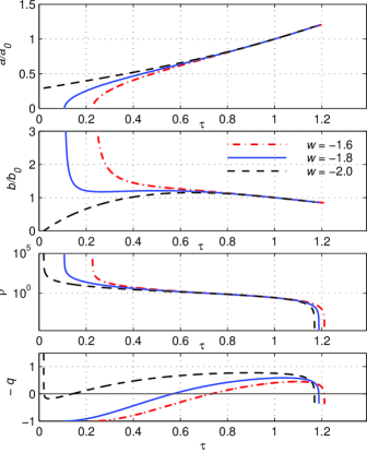
The results of calculation for scale factors $a(\tau)$, $b(\tau)$, density $\bar{\rho}(\tau)$ and the acceleration parameter

$$-q=\frac{\ddot{a}a}{{\dot{a}}^{2}}=\frac{A^{\prime\prime}+{A^{\prime}}^{2}}{{A^{\prime}}^{2}}$$ (25)

($q$ is the deceleration parameter) are presented in Fig. 1. Here $k_{1}=0$, $\Omega_{0}=0{.}27$, $\gamma=0{.}9$ and 3 scenarios for $w=-1{.}6$ (dash-dotted line), $w=-1{.}8$ (solid lines) and $w=-2$ (dashed lines) are shown.

This evolution begins from infinite value of density $\bar{\rho}$ at some initial moment $\tau_{0}$. We can see here two different variants for this beginning. For solutions with $w=-1{.}6$ and $w=-1{.}8$ (we denote them as “regular” solutions) the scale factor $a$ expands from $a=0$ like $a\sim\sqrt{\tau-\tau_{0}}$ at the initial stage whereas the scale factor $b$ diminishes from initial infinite value up to values $b\simeq b_{0}$ during some percent of total lifetime of this universe. This behavior of $b(\tau)$ looks like some variant of dynamical compactification, because the parameter $b_{0}$ is arbitrary one in this model, we may put $b_{0}$ to be sufficiently small.

Another type of evolution (“singular” solutions) is represented with dashed lines in Fig. 1 for $w=-2$. For singular solutions infinite value of density $\bar{\rho}$ at $\tau=\tau_{0}$ corresponds to nonzero value of the scale factor $a$ and $b=0$. Obviously, these solutions are nonphysical and should be excluded.

All regular and singular solutions in Fig. 1 describe accelerated expansion (for the factor $a$) at late stage of evolution. Beginning of this stage may be seen in the graph of the acceleration parameter $-q(\tau)$. Acceleration rate depends on the parameters $w$, $\gamma$, $\Omega_{0}$ and the curvature fraction (17) $\Omega_{k}=-k_{1}(a_{0}H_{0})^{-2}$ depending on the sign $k_{1}$. If $\Omega_{k}\neq 0$ ($k_{1}=\pm 1$), one should use the system (15) – (18) instead of Eqs. (19), (20). In this case we integrate numerically the function $A^{\prime}(\tau)$ simultaneously with solving the Cauchy problem for the system (15) – (18). We add here the natural initial condition $A\big{|}_{\tau=1}=0$ to conditions (22).

For all reasonable values of four free parameters $w$, $\gamma$, $\Omega_{0}$, $\Omega_{k}$ the stage of accelerated expansion appears to be finite, because density $\bar{\rho}$ inevitably vanishes in this model. In Fig. 1 this effect may be seen in the graphs $\bar{\rho}(\tau)$ with logarithmic scale in Y-direction. We denote the moment of zero density by $\tau_{*}$: $\bar{\rho}(\tau_{*})=0$. For $\tau>\tau_{*}$ density $\bar{\rho}$ becomes negative and nonphysical, all energy conditions (in particular, the weak energy condition) are violated.

This finite-time future singularity may be classified as the Type IV singularity in accordance with the scheme from Refs. BambaCapNO12 ; NojOdinFR . For this singularity $a(\tau_{*})$ is nonzero, $\bar{\rho}(\tau_{*})$ equals zero, the effective density and pressure

$$\rho_{eff}=\frac{3H^{2}}{8\pi G}=\rho_{c}{A^{\prime}}^{2},\quad p_{eff}=-\frac{2\dot{H}+3H^{2}}{8\pi G}=\frac{2q-1}{3}\rho_{eff}$$

remain nonzero, but higher derivatives of $H$ diverge at $\tau\to\tau_{*}$.

Note that the main features of the considered cosmological solutions, in particular, the future singularity, finite lifetime $\tau_{0}\leq\tau\leq\tau_{*}$ and negative density for $\tau>\tau_{*}$ take place not only for $d=1$, but also for higher dimensions $d\geq 2$. In the case of $d\geq 2$ additional dimensions after substituting the components $G^{\mu}_{\nu}$ into Einstein equation (4) and substitutions (12) in these equations and Eq. (10) we have in the flat case $k_{1}=k_{2}=0$ the following system PahwaChS , generalizing Eqs. (18) – (20):

$$A^{\prime\prime} = \frac{d(d-1)\,B^{\prime}\big{(}\frac{1}{2}B^{\prime}-A^{\prime}\big{)}-3(d+1)\,{A^{\prime}}^{2}-3d\bar{p}_{b}}{d+2},$$

$$\bar{\rho}^{\prime} = -3\bar{\rho}A^{\prime}-d(\bar{\rho}+\bar{p}_{b})\,B^{\prime},$$ (26)

$$B^{\prime} = \frac{\sqrt{3\big{[}(d+2)\,{A^{\prime}}^{2}+2(d-1)\,\bar{\rho}\big{]}/d}-3A^{\prime}}{d-1}.$$

Solutions of the system (26) for $d\geq 2$ were obtained in Ref. PahwaChS , but some features of them were not considered in that paper. For example, singular solutions with nonzero value $a(\tau_{0})$ (where $\bar{\rho}$ is infinite at the initial moment $\tau_{0}$) also take place for $d\geq 2$, if the value $w$ is less than the critical value $w_{cr}(\gamma,\Omega_{0})$. In Fig. 2 boundaries $w=w_{cr}$ separating domains of regular and singular solutions on the $\gamma,\,w$ plane are presented for different $d$ and $\Omega_{0}$. Singular solutions are described by the inequality $w<w_{cr}(\gamma,\Omega_{0})$ and lie below corresponding lines in Fig. 2.

Figure 2: Boundaries $w=w_{cr}$ between domains of regular (above) and singular solutions (below a curve) for indicated values $\Omega_{0}$ and $d$

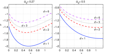
Another important property of these cosmological solutions is their finite-time future singularity, in other words, inevitability of “the end of the world” because of vanishing density at $\tau=\tau_{*}$ for all $d$ (see Fig. 4 below). The authors of Ref. PahwaChS did not pay attention to this phenomenon, essential for their model. It is connected with the chosen equation of state (21) for pressure $\bar{p}_{b}$ in extra dimensions. This drawback will be eliminated with modifying the model PahwaChS in Sect. IV after application this model to describing observational data for Type Ia supernovae in the next section.

III Application to supernovae observations

To apply the model to describing the observational data it is convenient, following the authors of PahwaChS , to use Internet table SuperTable for Type Ia supernovae in distant galaxies. At the present moment this updated table contains redshifts $z=z_{i}$, distance moduli $\mu_{i}$ and errors $\sigma_{i}$ of $\mu_{i}$ for $N=580$ supernovae.

Redshift

$$z=\frac{a_{0}}{a(t)}-1=e^{-A(\tau)}-1$$ (27)

is associated with the value of $a$ at the time $t$ of a supernova light emission. The distance modulus $\mu$ is the logarithmic function

$$\mu=5\log\frac{D_{L}}{10\,\,\mbox{pc}},$$

of the luminosity distance Clifton ; PahwaChS :

$$D_{L}=(1+z)\int\limits_{z}^{0}\!\frac{d\tilde{z}}{H(\tilde{z})}=\frac{a_{0}^{2}}{H_{0}a(\tau)}\,\int\limits_{\tau}^{1}\!\frac{d\tilde{\tau}}{a(\tilde{\tau})}.$$ (28)

To describe the data SuperTable of Type Ia supernovae, for given values $d$, $w$, $\gamma$, $\Omega_{0}$ of this model we consider evolution of the scale factor $a(\tau)$ and dependence of the numerical integral (28) $D_{L}$ and $\mu$ on $\tau$. For each value of redshift $z_{i}$ in the table SuperTable we calculate the corresponding $\tau=\tau_{i}$ with using Eq. (27) and linear approximation and the theoretical value $\mu_{th}=\mu(\tau_{i})$ for $\tau_{i}$ from Eq. (28). The measure of differences between these theoretical values $\mu_{th}=\mu_{th}(d,w,\gamma,\Omega_{0},\Omega_{k},z_{i})$ and the measured values $\mu_{i}$ is PahwaChS :

$$\chi^{2}(d,w,\gamma,\Omega_{0},\Omega_{k})=\sum_{i=1}^{N}\frac{\big{[}\mu_{i}-\mu_{th}(d,\dots,z_{i})\big{]}^{2}}{\sigma_{i}^{2}}.$$ (29)

The authors of Ref. PahwaChS calculated optimal parameters $w$ and $\gamma$, minimizing the function (29) for the flat model ($k_{1}=0$) with fixed $\Omega_{0}=0{.}27$ (23) and $d\geq 2$. In this approach for each $d\geq 2$ they minimized the function $\chi^{2}(w,\gamma)$ of two variables.

We generalize their approach to the case $d=1$ additional dimension. At the first step we fix $k_{1}=0$, $\Omega_{0}=0{.}27$ in according with Ref. PahwaChS and obtain the picture of level lines for the function $\chi^{2}(w,\gamma)$, presented in Fig. 3 for $d=1$ and $d=2$.

Figure 3: Level lines of $\chi^{2}(w,\gamma)$ for $k_{1}=0$, $\Omega_{0}=0{.}27$. The dashed line is the boundary of singular solutions

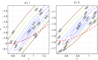
Here the dashed line is taken from Fig. 2 and separates regular and singular solutions. We see that for $d=1$ and $d=2$ the minimum of $\chi^{2}$ lies above this line, that is in the domain of regular solutions. The same picture also takes place for $d\geq 3$.

For each $d\geq 1$ we calculated minimums for the function of two variables $\chi^{2}(w,\gamma)$ and coordinates $w$, $\gamma$ of this minimum. They are represented in Table 1.

Table 1: Minimum of $\chi^{2}$ and optimal values $w$, $\gamma$ for fixed $k_{1}=0$, $\Omega_{0}=0{.}27$ and various $d$

$d$	1	2	3	6	10	$\Lambda$CDM
min $\chi^{2}$	563.15	563.41	563.52	563.65	563.7	563.29
$w$	$-1.77$	$-1.355$	$-1.212$	$-1.067$	$-1.01$	-
$\gamma$	0.925	0.819	0.772	0.715	0.686	-

We compare these minimal values with the value of the function (29) for the flat $\Lambda$CDM model with the same parameters $k_{1}=0$, $\Omega_{m}=\Omega_{0}=0{.}27$ (therefore, $\Omega_{\Lambda}=0{.}73$) and the same supernova data SuperTable . We see that the predictions are rather close, and for $d=1$ the model PahwaChS fits the data better than the flat $\Lambda$CDM model.

At the next step for more precise estimation of optimal model parameters we consider variations of fractions $\Omega_{0}=\Omega_{m}$ and $\Omega_{k}$ for matter density and curvature respectively. One should take into account these degrees of freedom in both models: the model PahwaChS and $\Lambda$CDM. In the model PahwaChS for each $d\geq 1$ we minimize the function (29) of four variables: $\chi^{2}(w,\gamma,\Omega_{0},\Omega_{k})$. We also compare this results with the same value of the $\Lambda$CDM model (where $\chi^{2}$ depends on $\Omega_{m}$ and $\Omega_{k}$) and keep in mind the constraints on these parameters due to cosmic microwave background anisotropy, galaxy clustering and other factors WMAP :

$$\Omega_{m}=0.2743\pm 0.0072,\quad-0.0133<\Omega_{k}<0.0084.$$ (30)

Numerical search of this minimum includes a starting point (for example, the values from Table 1), analysis of gradients or increments for $\chi^{2}$ and the constraints (30). The results of calculation with optimal values of the model parameters are presented in Table 2.

Table 2: Minimum of $\chi^{2}$ and optimal values $w$, $\gamma$, $\Omega_{0}$, $\Omega_{k}$

$d$	1	2	3	6	10	$\Lambda$CDM
min $\chi^{2}$	563.136	563.39	563.506	563.634	563.69	563.058
$w$	$-1{.}740$	$-1.323$	$-1.2032$	$-1.061$	$-1.003$	-
$\gamma$	0.926	0.821	0.7739	0.7174	0.696	-
$\Omega_{0}$	0.2815	0.279	0.274	0.2673	0.267	0.2716
$\Omega_{k}$	0.0084	0.0084	0.0084	0.0084	0.0084	$-0.0133$

We see that the $\Lambda$CDM model is more sensitive to variations of $\Omega_{m}$ and $\Omega_{k}$ and the better result for this model is achieved. Here optimal values of the model parameters are determined by the constraints (30). We impose these constraints on the model PahwaChS though they are not strictly applicable to it. In this model min $\chi^{2}$ weakly depends on $\Omega_{0}$ and $\Omega_{k}$, so we can not diminish $\chi^{2}$ appreciably if we slightly broaden the limitations (30).

In Fig. 4 one can see evolution of the scale factor $a(\tau)$, (and $b$ for the model PahwaChS ), the acceleration parameter $-q(\tau)$ and density $\bar{\rho}(\tau)$ for the $\Lambda$CDM model and the model PahwaChS with $d=1$ (solid lines), $d=2$ (dots) and $d=6$ (dash-dotted lines). For all these models we use the optimal parameters from Table 2.

Figure 4: Scale factors $a(\tau)$, $b(\tau)$, acceleration parameter $-q(\tau)$ and density $\bar{\rho}(\tau)$ for the optimal solutions from Table 2

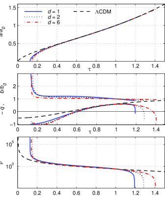
Evolution of the scale factor $a(\tau)$ for the model PahwaChS with different $d$ and for the $\Lambda$CDM model is very close up to $z\simeq 1{.}5$ ($a>0{.}4a_{0}$), before this epoch the $\Lambda$CDM model demonstrates slower expansion. This difference is more visible for the acceleration graphs $-q(\tau)$. The scale factor $b$ for the case PahwaChS diminishes to $b\simeq b_{0}$ according to the mentioned above compactification scheme (compare with the regular solutions in Fig. 1).

Behavior of cosmological solutions in the future for both models is also different. The $\Lambda$CDM model demonstrates unlimited accelerated expansion whereas for the model PahwaChS the acceleration turns into deceleration and inevitability results in the above mentioned zero density $\bar{\rho}$ at $\tau=\tau_{*}$ with nonphysical values $\bar{\rho}<0$ for $\tau>\tau_{*}$. The finite lifetime of this universe depends on $d$, it is the smallest for $d=1$. In the next section we discuss how to eliminate this essential drawback of the model.

IV Modification of the model

We have noted that all cosmological solutions in the model PahwaChS have the finite-time future singularity. This inevitable “end of the world” is connected with the chosen power law dependence (21) of pressure $\bar{p}_{b}$ in extra dimensions on density $\bar{\rho}$. The terms with the factor $\bar{p}_{b}$ in equations (20) for $d=1$ or (26) for $d>1$ determine rate of density decreasing when $\bar{\rho}$ is small at the end of its evolution. In this case the leading terms in the mentioned equations are

$$\bar{\rho}^{\prime}\simeq\left\{\begin{array}[]{ll}\bar{p}_{b}A^{\prime},&d=1,\\ -d\bar{p}_{b}B^{\prime},&d>1,\end{array}\right.\qquad\bar{\rho}\to 0.$$ (31)

For $\bar{\rho}\to 0$ we have nonzero values $A^{\prime}$ and $B^{\prime}$, so for the weak power law dependence (21) the approximate equation (31) $\bar{\rho}^{\prime}\simeq-C{\bar{\rho}}^{1-\gamma}$ has the finite solution

$$\bar{\rho}\simeq\big{[}\gamma C(\tau_{*}-\tau)\big{]}^{1/\gamma}.$$ (32)

To avoid this finiteness we are to modify the equation of state (power law dependence) (21) of the model PahwaChS for small $\bar{\rho}$. In particular, a linear dependence for $\bar{\rho}$ close to zero

$$\bar{p}_{b}=w_{0}\bar{\rho},\qquad\bar{\rho}\to 0$$ (33)

ensures infinite evolution with positive density.

The linear law (33) for all $\bar{\rho}$ does not describe the observed accelerated expansion. For good agreement with observations we are to search an equation of state $\bar{p}_{b}(\bar{\rho})$ with slower growth of $|\bar{p}_{b}|$ at high $\bar{\rho}$ similar to Eq. (21). We suggest the appropriate variant of this dependence

$$\bar{p}_{b}=\bigg{(}w_{1}+\frac{w}{\rho_{0}+\bar{\rho}}\bigg{)}\bar{\rho}$$ (34)

with the linear law (33) for $\bar{\rho}\ll\rho_{0}$ (here $w_{0}=w_{1}+w/\rho_{0}$) and another linear law $\bar{p}_{b}\simeq w_{1}\bar{\rho}$ for $\bar{\rho}\gg\rho_{0}$.

The model (15) – (18) or (26) for $d>1$ with the linear-fractional equation of state (34) makes it possible to avoid finite lifetime of the type (32) and to transform it into the exponential asymptotic behavior

$$\bar{\rho}\sim\exp(-C\tau),\qquad C=\mbox{const}\cdot\Big{(}w_{1}+\frac{w}{\rho_{0}}\Big{)}.$$ (35)

This behavior results from the equation $\bar{\rho}^{\prime}\simeq-C{\bar{\rho}}$ and may be observed in graphs $\bar{\rho}(\tau)$ in Fig. 5.

For the model with Eq. (34) we can find optimal values of parameters $w$, $w_{1}$, $\rho_{0}$, $\Omega_{0}$, $\Omega_{k}$ presented in Table 3 and achieve better agreement with the supernovae data SuperTable than for the models $\Lambda$CDM and PahwaChS with Eq. (21). Cosmological solutions for the model with Eq. (34) and parameters from Table 3 are shown in Fig. 5.

Table 3: Optimal parameters for the model with Eq. (34), $\rho_{0}=0{.}005$ is fixed

$d$	1	2	3	6	10	$\Lambda$CDM
min $\chi^{2}$	562.898	562.814	562.79	562.766	562.757	563.058
$w$	$-1.603$	$-1.026$	$-0.84$	$-0.658$	$-0.587$	-
$w_{1}$	$-0{.}195$	$-0.343$	$-0{.}387$	$-0{.}426$	$-0{.}439$	-
$\Omega_{0}$	$0{.}2815$					0.2716
$\Omega_{k}$	$-0.0133$					$-0.0133$

We see in Table 3 that the accuracy of the model with Eq. (34) increases ($\chi^{2}$ diminishes) for large $d$, unlike in the case with Eq. (21) in Table 2. We should note that the values $\chi^{2}$ in Table 3 are not absolutely minimal, because we fixed the parameter $\rho_{0}=0{.}005$. It is interesting, that for all $d$ we can achieve smaller values min $\chi^{2}$, if we take smaller values of $\rho_{0}$. But if $\rho_{0}\to 0$, the factor $C$ in the exponent (35) tends to infinity, the density $\bar{\rho}$ decreases too rapidly and the picture of vanishing $\bar{\rho}$ looks like in the finite case in Fig. 4. So we put the restriction $\rho_{0}\geq 0{.}005$ to exclude this almost instantaneous transition to the state with $\bar{\rho}\simeq 0$. Under this constraint we have the optimal value $\rho_{0}=0{.}005$ and also $\Omega_{0}=0{.}2815$, $\Omega_{k}=-0.0133$ for all $d$.

Fig. 5 demonstrates cosmological solutions for the model with Eq. (34) with the optimal values of parameters from Table 3. For both models Eqs. (34) and (21) in Figs. 4 and 5 the acceleration epoch is finite and its duration depends on $d$ in the same manner. But after this epoch for the model with Eq. (34) we see here infinite decelerated expansion.

Figure 5: Scale factors $a(\tau)$, $b(\tau)$, functions $-q(\tau)$ and $\bar{\rho}(\tau)$ for the model with Eq. (34) with the parameters from Table 3

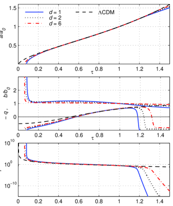
Graphs of $a(\tau)$, $-q(\tau)$ and $\bar{\rho}(\tau)$ here are more close to the dashed lines for the $\Lambda$CDM model during the acceleration epoch than the similar curves in Fig. 4. But after the mentioned epoch predictions of the $\Lambda$CDM model and the model (34) sharply diverge.

In Fig. 6 we present how the model with Eq. (34) for $d=1$, 2, 6 and the $\Lambda$CDM model describe the supernovae data from the site SuperTable (dots) in the $z$-$D_{L}$ plane. All these models were considered below in Fig. 5, we use the same optimal parameters from Table 3 and the same notations for the curves, in particular, the dashed line for the $\Lambda$CDM model.

Figure 6: Luminosity distance $D_{L}$ in Gpc depending on redshift $z$ for the models $\Lambda$CDM and (34) with parameters from Table 3. Dots are the data SuperTable

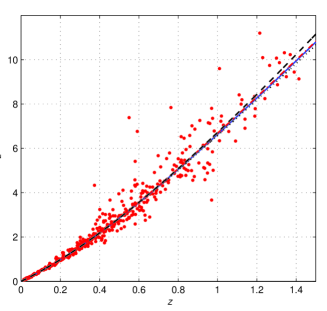
The presented curves are very close in the region $z<1$, for larger $z$ the $\Lambda$CDM line slightly diverges from others. These lines are result of optimal fitting to the observational data SuperTable (580 dots in Fig. 6). The values $\chi^{2}$ in Table 3 show rather good results for the model PahwaChS with Eq. (34) for pressure, but these values are not the best fit, because we fixed $\rho_{0}$ to avoid the mentioned above sharp transition to $\bar{\rho}\simeq 0$.

V Conclusion

The gravitational model of Pahwa, Choudhury and Seshadri PahwaChS with additional spatial dimensions and anisotropic pressure provides accelerated expansion of the universe corresponding to observational data for Type Ia supernovae SuperTable simultaneously with dynamical compactification of $d$ extra dimensions. It is important that such a behavior of solutions results from rather simple equations of state (21). This approach is more natural in comparison with the scheme of Mohammedi Mohammedi02 , where complicated equations of state are deduced from the constructed solutions, in particular, from the solution (36) described below.

The authors of Ref. PahwaChS did not consider the case $d=1$, but we found that for the chosen in Ref. PahwaChS power law equation of state (21) it is the case $d=1$ that yields the best fit (see Tables 1, 2).

Unfortunately, the model PahwaChS with the power law dependence (21) inevitably predicts the finite-time future singularity of Type IV in classification from Refs. BambaCapNO12 ; NojOdinFR . It is connected with vanishing density $\bar{\rho}$ at finite time $\tau=\tau_{*}$ (and negative density for $\tau>\tau_{*}$). Evolution of this universe is broken at $\tau_{*}$, the finite lifetime is shorter for small $d$ (see Fig. 4). We demonstrated in Sect. IV, that this drawback has technical nature. It is connected with too weak dependence $\bar{p}_{b}(\bar{\rho})$ for small $\bar{\rho}$ in the power law equation of state (21). If we modify this law and choose a linear dependence (33) for small $\bar{\rho}$, we obtain an infinite cosmological evolution with positive density (but vanishing at $\tau\to\infty$). We suggest the linear-fractional variant (34) of dependence $\bar{p}_{b}(\bar{\rho})$ to solve the following two problems: (a) to avoid “the end of the world” of the type (32) and (b) to describe 580 Type Ia supernovae data points from the site SuperTable . The dependence (34) is a bit more complicated than Eq. (21), but it successfully conserves positive density $\bar{\rho}$ during infinite lifetime and fits the data SuperTable better than the $\Lambda$CDM model and the model from Ref. PahwaChS with Eq. (21). Although the simplicity of the equations of state (3) is the important advantage of the model PahwaChS , we are to step back from this simplicity. But in our opinion, the dependence (34) is the minimal retreat that solves this problem.

Our calculations should be compared with predictions of other multidimensional models PahwaChS ; Mohammedi02 ; Darabi03 ; Darabi09 ; BringmannEG03 ; PanigrahiZhCh06 ; MiddleSt11 ; FarajollahiA10 ; Neupane . We shall consider the models, describing the late time acceleration of $a(t)$ together with a contraction of $b(t)$, in particular, the Mohammedi model in Ref. Mohammedi02 with the ansatz (6) $b/b_{0}=(a/a_{0})^{-n}$. It ensures a dynamical compactification, if $n$ is positive and $a(t)$ expands. For $n$ satisfying the equality

$$dn(dn-n-6)+6=0$$

a set of solutions with accelerated expansion was obtained in Ref. Mohammedi02 in the form

$$a/a_{0}=C_{1}\exp(\mu t)-C_{2}\exp(-\mu t)$$

$$=\tilde{C}_{1}\exp(\tilde{\mu}\tilde{\tau})+(1-\tilde{C}_{1})\exp(-\tilde{\mu}\tilde{\tau}).$$ (36)

Here $\tilde{\tau}=\tau-1$, the natural condition $a\big{|}_{t=t_{0}}=a_{0}$ must be saticfied.

We mentioned above, that the equation of state in the Mohammedi’s approach may be determined at the last stage after substitution of the expressions (36) and (6) into Eqs. (4) with a $\Lambda$ term. In particular, the relation between $P_{a}$ and $\rho$ for solutions (36) results from the first two equations (4) (in our notations)

$$\begin{array}[]{c}3k_{1}/a^{2}-\Lambda=8\pi G\rho,\\ \big{[}4C_{1}C_{2}\mu^{2}(2-2dn-dn^{2})-k_{1}\big{]}/a^{2}\rule{0.0pt}{13.00005pt}\\ -dn(n+1)\,\mu^{2}+\Lambda=8\pi GP_{a},\rule{0.0pt}{13.00005pt}\end{array}$$

if we exclude $a^{2}$. This equation of state is mush more complicated than its analog $P_{a}=0$ for the model PahwaChS , in addition it has the negative limit of $P_{a}$ at $a\to\infty$ for the case $\Lambda=0$.

If we accept these complicated equations of state for the model Mohammedi02 , we can obtain the optimal solution (36), minimizing the sum $\chi^{2}$ (29) for the same supernovae data SuperTable . For this purpose we use 2 fitting parameters of these solutions: $\tilde{C}_{1}$ and $\tilde{\mu}$. The calculations result in the optimal values $\tilde{C}_{1}=1{.}229$, $\tilde{\mu}=0{.}679$ and the corresponding minimum $\chi^{2}\simeq 564{.}4$. This minimum is close to the results of the considered model PahwaChS in Tables 2 and 3. So we may conclude that the solution (36) describes the supernovae data SuperTable rather successfully. It is interesting that solutions close to Eq. (36) appeared in Refs. Neupane in the brane model.

In Refs. Darabi03 ; Darabi09 Darabi obtained exponential solutions $a=C_{1}\exp(\mu t)$ for the model with varying $\Lambda\sim a^{-m}$. Such a solution with one fitting parameter is less adaptable in comparison with Eq. (36), the optimal sum (29) in this case $\chi^{2}>955$.

Note that in this paper for the model with Eq. (34) we practically used only two fitting parameters $w$ and $w_{1}$. The value $\rho_{0}$ was fixed because for very small $\rho_{0}$ we have better fit, but the sharp downfall of $\bar{\rho}(\tau)$ to $\bar{\rho}\simeq 0$ looks like the mentioned “end of the world”. The parameters $\Omega_{0}$ and $\Omega_{k}$ influence on minimum of $\chi^{2}$ rather weakly for the model with Eq. (34). If we fix, for example, $\Omega_{0}=0{.}27$ and $\Omega_{k}=0$, minimums for $\chi^{2}$ will differ from results in Table 3 less then 0.01 for all $d$.

Cosmological solutions in the model with Eq. (34) are divided into regular and singular ones similarly to solutions with Eq. (21) shown in Fig. 1. However, Fig. 5 demonstrates that for the optimal values of parameters from Table 3 solutions with Eq. (34) are regular.

It is interesting that the model PahwaChS with both considered variants of dependence $\bar{p}_{b}$ on $\bar{\rho}$ (21) and (34) predicts finiteness of the acceleration epoch. Its duration depends on $d$ in the same manner (compare Figs. 4 and 5) and then acceleration sharply turns to deceleration. In the case (21) this evolution is broken at $\tau=\tau_{*}$ with $\bar{\rho}(\tau_{*})=0$, but for the model with Eq. (34) the decelerated expansion is infinite and density $\bar{\rho}(\tau)$ tends to zero in the exponential form (35).

References

- (1) S. Perlmutter et al., Astrophys. J. 517 (1999) 565, astro-ph/9812133.
- (2) A. G. Riess et al., Astron. J. 116 (1998) 1009, astro-ph/9805201.
- (3) E. Komatsu et al., Astrophys. J. Suppl. 192 (2011) 18, arXiv:1001.4538 [astro-ph.CO].
- (4) B. A. Reid et al., MNRAS 404 (2010) 60, arXiv:0907.1659 [astro-ph.CO].
- (5) E. J. Copeland, M. Sami and S. Tsujikawa, Int. J. Mod. Phys. D 15 (2006) 1753, hep-th/0603057.
- (6) T. Clifton, P. G. Ferreira, A. Padilla and C. Skordis, Physics Reports 513 (2012) 1, arXiv:1106.2476 [astro-ph.CO].
- (7) K. Bamba, S. Capozziello, S. Nojiri and S. D. Odintsov, Astrophys. and Space Science 342 (2012) 155, arXiv:1205.3421 [gr-qc].
- (8) M. Kunz, Comptes rendus - Physique 13 (2012) 539, arXiv:1204.5482 [astro-ph.CO].
- (9) D. Sahdev, Phys. Rev. D 30 (1984) 2495.
- (10) I. Pahwa, D. Choudhury and T. R. Seshadri, J. of Cosmology and Astroparticle Phys. 1109 (2011) 015, arxiv:1104.1925 [gr-qc].
- (11) N. Mohammedi, Phys. Rev. D 65 (2002) 104018, hep-th/0202119.
- (12) F. Darabi, Class. Quant. Grav. 20 (2003) 3385, gr-qc/0301075.
- (13) F. Darabi, arXiv:0902.1863 [gr-qc].
- (14) T. Bringmann, M. Eriksson and M. Gustafsson, Phys. Rev. D 68 (2003) 063516, astro-ph/0303497.
- (15) D. Panigrahi, Y. Z. Zhang and S. Chatterjee, Int. J. Mod. Phys. A 21 (2006) 6491, gr-qc/0604079.
- (16) C. A. Middleton and E. Stanley, Phys. Rev. D 84 (2011) 085013, arXiv:1107.1828 [gr-qc].
- (17) H. Farajollahi, H. Amiri, Int. J. Mod. Phys. D 19 (2010) 1823, arXiv:1005.3140 [gr-qc].
- (18) I. P. Neupane, Class. Quant. Grav. 26 (2009) 195008, arXiv:0905.2774; Int. J. Mod. Phys. D 19 (2010) 2281, arXiv:1004.0254 [gr-qc].
- (19) Li-e Qiang, Y. Ma, M. Han and D. Yu, Phys. Rev. D 71 (2005) 061501, gr-qc/0411066.
- (20) J. Ponce de Leon, JCAP 03 (2010) 030, arXiv:1001.1961 [gr-qc].
- (21) R. Maartens and K. Koyama, Living Rev. Rel. 13 (2010) 5, arXiv:1004.3962 [hep-th].
- (22) A. Y. Kamenshchik, U. Moschella and V. Pasquier, Phys. Lett. B 511 (2001) 265, gr-qc/0103004.
- (23) V. Gorini, A. Y. Kamenshchik and U. Moschella, Phys. Rev. D 67 (2003) 063509, astro-ph/0209395.
- (24) R. R. Caldwell, R. Dave and P. J. Steinhardt, Phys. Rev. Lett. 80 (1998) 1582, astro-ph/9708069.
- (25) C. Armendáriz-Picón, V. F. Mukhanov and P. J. Steinhardt, Phys. Rev. Lett. 85 (2000) 4438, astro-ph/0004134.
- (26) J. Khoury and A. Weltman, Phys. Rev. D 69 (2004) 044026, astro-ph/0309411.
- (27) T. P. Sotiriou and V. Faraoni, Rev. of Modern Phys. 82 (2010) 451, arXiv:0805.1726 [gr-qc].
- (28) S. Nojiri and S. D. Odintsov, Phys. Rept. 505 (2011) 59, arxiv:1011.0544 [gr-qc].
- (29) Supernova Cosmology Project, http://supernova.lbl.gov/Union/