Quantum fidelity for degenerate groundstates in quantum phase transitions

Abstract

Spontaneous symmetry breaking mechanism in quantum phase transitions manifests the existence of degenerate groundstates in broken symmetry phases. To detect such degenerate groundstates, we introduce a quantum fidelity as an overlap measurement between system groundstates and an arbitrary reference state. This quantum fidelity is shown a multiple bifurcation as an indicator of quantum phase transitions, without knowing any detailed broken symmetry, between a broken symmetry phase and symmetry phases as well as between a broken symmetry phase and other broken symmetry phases, when a system parameter crosses its critical value (i.e., multiple bifurcation point). Each order parameter, characterizing a broken symmetry phase, from each of degenerate groundstates is shown similar multiple bifurcation behavior. Furthermore, to complete the description of an ordered phase, it is possible to specify how each order parameter from each of degenerate groundstates transforms under a symmetry group that is possessed by the Hamiltonian because each order parameter is invariant under only a subgroup of the symmetry group although the Hamiltonian remains invariant under the full symmetry group. Examples are given in the quantum $q$-state Potts models with a transverse magnetic field by employing the tensor network algorithms based on infinite-size lattices. For any $q$, a general relation between the local order parameters is found to clearly show the subgroup of the $Z_{q}$ symmetry group. In addition, we systematically discuss the criticality in the $q$-state Potts model.

I Introduction

Quantum phase transitions (QPTs) have attracted much attention to understand a relationship with quantum information QPT ; Chaikin . Compared to local order parameters in the conventional Landau-Ginzburg-Wilson paradigm based on the spontaneous symmetry breaking mechanism, in connections between quantum information and QPTs, quantum entanglement, i.e., a purely quantum correlation being absent in classical systems, can be used as an indicator of QPTs driven by quantum fluctuations in quantum many-body systemsLandau . Quantum fidelity, based on the basic notions of quantum mechanics on quantum measurement, has also provided an another way to characterize QPTsZhou1 ; Rams ; Mukherjee ; Zanardi . In the last few years, various quantum fidelity approaches such as fidelity per lattice site (FLS)Zhou1 , reduced fidelityLiu , fidelity susceptibilityGu , density-functional fidelityGu , and operator fidelityXiao , have been suggested and implemented to explore QPTs.

Actually, the fidelity is a measure of similarity between two quantum states by defining a overlap function between them. The fact that groundstates in different phases should be orthogonal due to their distinguishability in the thermodynamic limit allows a fidelity between quantum many-body states in different phases signaling QPTs because an abrupt change of the fidelity is expected across a critical point in the thermodynamic limit Zhou1 ; Rams ; Mukherjee ; Liu ; Gu ; Xiao ; Zanardi . Thus, the fidelity has great advantages to characterize the QPTs in a variety of quantum lattice systems because the groundstate of a system undergoes a drastic change in its structure at a critical point, regardless of of what type of internal orders are present in quantum many-body states. Especially, the groundstate FLS has been manifested to capture drastic changes of the groundstate wave functions around a critical point even for those cannot be described in the framework of Landau-Ginzburg-Wilson theory, such as a Beresinskii-Kosterlitz-Thouless (BKT) transtion and topological QPTs in quantum lattice many-body systems Wang .

Even though such latest advances in understanding QPTs have been made significantly, however, understanding directly degenerate groundstates originated from a spontaneous symmetry breaking as a heart of the Landau-Ginzburg-Wilson theory has still been remained in unexplored research regimes. Also, recently developed tensor network (TN) algorithmsmps ; DMRG ; Vidal ; Zhou2 in quantum lattice systems have made it possible to explore directly degenerate groundstates with a randomly chosen initial state subject to an imaginary time evolution. Based on the tensor network algorithm, indeed, Zhao et al. Zhao , for the first time, have detected a doubly degenerate groundstate by means of FLS bifurcations in quantum Ising model and spin-1/2 XYX model with transverse magnetic field. Also, in various spin lattice models Bi , a doubly degenerate groundstate has been detected. Further, in the quantum three-state Potts model Dai , a three-fold degenerate groundstate has been detected by using a bifurcation of FLS and a probability mass distribution function.

When the system has more than three-fold degenerate groundstates, the degenerate groundstates are orthogonal one another in the thermodynamic limit. A quantum fidelity defined by a overlap function between degenerate groundstates may not distinguish all the degenerate groundstates properly. Then, in this paper, we investigate how to detect generally $N$-fold degenerate groundstates calculated from a tensor network algorithm. To do this, we introduce a quantum fidelity between degenerate groundstates and an arbitrary reference state. The quantum fidelity corresponds to a projection of each groundstate onto the chosen reference state. Straightforwardly, for a broken symmetry phase, the number of different projection magnitudes denotes the groundstate degeneracy. At a critical point, the different projection magnitudes collapse to one projection magnitude. In such a property of the defined quantum fidelity, the different projection magnitudes of the groundstates can be called as multiple bifurcation of the quantum fidelity. A multiple bifurcation point is identified to be a critical point.

As a prototypical example, we explore the groundstate wavefunctions in the $q$-state Potts modelPotts ; Wu in transverse magnetic fields. By employing the infinite matrix product state (iMPS) with the time evolving block decimation (iTEBD) method Vidal , we calculate the groundstates of the model. Due to the broken $Z_{q}$ symmetry, the $q$-fold degenerate groundstates in the broken symmetry phase are obtained by means of the quantum fidelity with $q$ branches. A continuous (discontinuous) QPT for $q\leq 4$ ($q>4$) has been manifested by a continues (discontinuous) fidelity function across the critical point. The multiple bifurcation points are shown to correspond to the critical points. Also, we discuss a multiple bifurcation of local order parameters and its characteristic properties for the broken symmetry phase. We find a general relation between the order parameters from each of degenerate groundstates. The general relation shows clearly how the order parameters from each of the degenerate groundstates transform under the subgroup of the symmetry group $Z_{q}$. In addition, for $q=4$, we calculate the critical exponents agree well with their exact values. From the finite-entanglement scalings of the von Neumann entropy and the correlation length, the cental charges are calculated to classify the universal classes for each $q$-state Potts model.

This paper is organized as follows. In Sec.II, we briefly explain the iMPS representation and the iTEBD method in one-dimensional quantum lattice systems. In Sec. III, the $q$-state Potts model is introduced. Section IV devotes how to detect degenerate groundstate by using a quantum fidelity between the degenerate groundstates and a reference state. By using the quantum fidelity per lattice site, the quantum phase transitions are discussed based its multiple bifurcations and multiple bifurcation points indicating quantum critical points in Sec. V. In Sec. VI, to complete the description of the ordered phases, we discuss the magnetizations given from the degenerate groundstates and obtain a general relation between them. Section VII presents the critical exponents for $q=4$ and the central charges for $q=3$ and $q=4$. Also, we discuss the quantum phase transitions from the von Neumann entropies. Finally, our summary is given in Sec. VIII.

II Numerical method: IMPS approach

Recently, significant progress has been made in numerical studies based on TN representations for the investigation of quantum phase transitionsmps ; DMRG ; Vidal ; Murg , which offers a new perspective from quantum entanglement and fidelity, thus providing a deeper understanding on characterizing critical phenomena in finite and infinite spin lattice systems. Actually, a wave function represented in TNs allows to perform the classical simulation of quantum many-body systems. Especially, in one-dimensional spin systems, a wave function for infinite-size lattices can be described by the iMPS representationVidal . which has been successfully applied to investigate the properties of groundstate wave functions in various infinite spin lattice systemsWang ; Liu .

For an infinite one-dimensional lattice system, a state can be written asVidal

$$|\Psi\rangle=\sum_{\{S\}}\sum_{\{\alpha\}}\cdots\lambda^{[i]}_{\alpha_{i}}\Gamma^{[i]}_{\alpha_{i},s_{i},\alpha_{i+1}}\lambda^{[i+1]}_{\alpha_{i+1}}\Gamma^{[i+1]}_{\alpha_{i+1},s_{i+1},\alpha_{i+2}}\lambda^{[i+2]}_{\alpha_{i+2}}\cdots$$

$$~{}\hskip 56.9055pt\times|\cdots S_{i-1}S_{i}S_{i+1}\cdots\rangle,$$ (1)

where $|S_{i}\rangle$ denote a basis of the local Hilbert space at the site $i$, the elements of a diagonal matrix $\lambda^{[i]}_{\alpha_{i}}$ are the Schmidt decomposition coefficients of the bipartition between the semi-infinite chains $L(-\infty,...,i)$ and $R(i+1,...,\infty)$, and $\Gamma^{[i]}_{\alpha_{i},S_{i},\alpha_{i+1}}$ are a three-index tensor. The physical indices $S_{i}$ take the value $1,\cdots,d$ with the local Hilbert space dimension $d$ at the site $i$. The bond indices $\alpha_{i}$ take the value $1,\cdots,\chi$ with the truncation dimension of the local Hilbert space at the site $i$. The bond indices connect the tensors $\Gamma$ in the nearest neighbor sites. Such a representation in Eq. (1) is called the iMPS representation. If a system Hamiltonian has a translational invariance, one can introduce a translational invariant iMPS representation for a state. Practically, for instance, for a two-site translational invariance, the state can be reexpressed in terms of only the three-index tensors $\Gamma_{A(B)}$ and the two diagonal matrices $\lambda_{A(B)}$ for the even (odd) sites, where $\{\Gamma,\lambda\}$ are in the canonical form, i.e.,

$$|\Psi\rangle=\sum_{\{S\}}\sum_{\{l,r\}}\cdots\lambda_{A}\Gamma_{A}\lambda_{B}\Gamma_{B}\lambda_{A}\cdots|\cdots S_{i-1}S_{i}S_{i+1}\cdots\rangle,$$ (2)

where $l$ and $r$ are the left and right bond indices, respectively.

Once a random initial state $|\Psi(0)\rangle$ is prepared in the iMPS representation, one may employ the iTEBD algorithm to calculate a groundstate wavefunction numerically. For instance, if a system Hamiltonian is translational invariant and the interaction between spins consists of the nearest-neighbor interactions, i.e., the Hamiltonian can be expressed by $H=\sum_{i}h^{[i,i+1]}$, where $h^{[i,i+1]}$ is the nearest-neighbor two-body Hamiltonian density, a groundstate wavefunction of the system can be expressed in the form in Eq. (2). The imaginary time evolution of the prepared initial state $|\Psi(0)\rangle$, i.e.,

$$|\Psi(\tau)\rangle=\frac{\exp[-H\tau]|\Psi(0)\rangle}{||\exp[-H\tau]|\Psi(0)\rangle||},$$ (3)

leads to a groundstate of the system for a large enough $\tau$. By using the Suzuki-Trotter decompositionsuzuki , actually, the imaginary time evolution operator $U=\exp[-H\tau]$ can be reduced to a product of two-site evolution operators $U(i,i+1)$ that only acts on two successive sites $i$ and $i+1$. For the numerical imaginary time evolution operation, the continuous time evolution can be approximately realized by a sequence of the time slice evolution gates $U(i,i+1)=\exp\left[-h^{[i,i+1]}\delta\tau\right]$ for the imaginary time slice $\delta\tau=\tau/n\ll 1$. A time-slice evolution gate operation contracts $\Gamma_{A}$, $\Gamma_{B}$, one $\lambda_{A}$, two $\lambda_{B}$, and the evolution operator $U(i,i+1)=\exp\left[-h^{[i,i+1]}\delta\tau\right]$. In order to recover the evolved state in the iMPS representation, a singular value decomposition (SVD) is performed and the $\chi$ largest singular values are obtained. From the SVD, the new tensors $\Gamma_{A}$, $\Gamma_{B}$, and $\lambda_{A}$ are generated. The latter is used to update the tensors $\lambda_{A}$ as the new one for all other sites. Similar contraction on the new tensors $\Gamma_{A}$, $\Gamma_{B}$, two new $\lambda_{A}$, one $\lambda_{B}$, and the evolution operator $U(i+1,i+2)=\exp\left[-h^{[i+1,i+2]}\right]$, and its SVD produce the updated $\Gamma_{A}$, $\Gamma_{B}$, and $\lambda_{B}$ for all other sites. After the time-slice evolution, then, all the tensors $\Gamma_{A}$, $\Gamma_{B}$, $\lambda_{A}$, and $\lambda_{B}$ are updated. This procedure is repeatedly performed until the system energy converges to a groundstate energy that yields a groundstate wavefunction in the iMPS representation. The normalization of the groundstate wavefunction is guaranteed by requiring the norm $\langle\Psi|\Psi\rangle=1$. Finally, one can determine how many groundstates exist for a fixed system parameters with different initial states. Once a system undergoes a spontaneous symmetry breaking, the iMPS algorithm can automatically produce degenerate groundstates with randomly chosen initial states for the broken symmetry phase. It has been manifested by successfully detecting a doubly degenerate groundstates from $Z_{2}$ broken symmetry phases in various spin systems such as quantum Ising model, spin-1/2 XYX with transverse magnetic field, and a one-dimensional spin model with competing two-spin and three-spin interactions Zhao ; Bi . However, it has not been discussed yet how to detect an $N$-fold degenerate groundstates. In the following sections, we discuss this issue clearly by introducing the $q$-state Potts model that may have a $q$-fold generate groundstate in broken symmetry phases.

III Quantum $q$-state Potts model

In the lattice statistical mechanics, the quantum $q$-state Potts model is one of the most important models as a generalization of the Ising model ($q=2$)Baxter2 ; Wu . The $q$-state Potts model has the very intriguing critical behavior that has become an important testing platform for different numerical and analytical methods and approaches in studying critical phenomenaWu ; Nijs ; Pearson ; Black ; Caselle ; Hove . As is well-known in Ref. Wu, , the quantum q-state Potts model exhibits a continuous quantum phase transition for $q\leq 4$ and a first-order (discontinuous) phase transition for $q>4$ at the critical point.

We consider the $q$-state quantum Potts model in a transverse magnetic field $\lambda$ on an infinite-size lattice:

$$H_{q}=-\sum_{j=1}^{\infty}\sum^{q-1}_{p=1}\Bigg{(}M_{x,\,p}(j)~{}M_{x,\,q-p}(j+1)+\lambda M_{z}(j)\Bigg{)},$$ (4)

where $\lambda$ is the transverse magnetic field and $M_{x/z,p}(i)$ with $p\in[1,q-1]$ are the $q$-state Potts spin matrices at the lattice site $j$. The $q$-state Potts spin matrices are given as

$$M_{x,1}=\left(\begin{array}[]{ccccc}0&I_{q-1}\\ 1&0\end{array}\right)\mbox{~{}and~{}}M_{z}=\left(\begin{array}[]{ccccc}q-1&0\\ 0&I_{q-1}\end{array}\right),$$

where $I_{q-1}$ is the $(q-1)\times(q-1)$ identity matrix and $M_{x,p}=(M_{x,1})^{p}$. As is known, the model Hamiltonian has a $Z_{q}$ symmetryWu . If the groundstate of the Hamiltonian does not preserve the $Z_{q}$ symmetry, the system undergoes the $Z_{q}$ symmetry breaking, i.e., a QPT. Specifically, when the magnetic filed changes across $\lambda_{c}=1$, the $q$-state Potts model undergoes a QPT between an ordered phase and a disordered phase. The QPT is originated from the $Z_{q}$ symmetry breaking which results in the emergence of long-range order and the $q$ degenerate groundstates in the ordered phase.

IV Degenerate groundstates and quantum fidelity

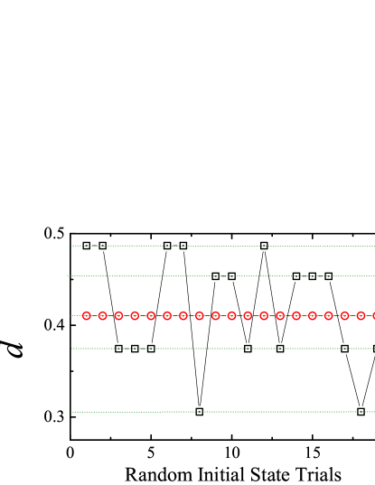
Figure 1: (Color online) Groundstate quantum FLS $d$ for the $4$-state Potts model with an arbitrary reference state as a function of random initial state trials. Here, $|\phi\rangle$ is an arbitrary reference state, the numerical groundstates $|\psi\rangle$ are in the broken symmetry phase with $\lambda=0.8$, and $|\varphi\rangle$ is in the symmetry phase with $\lambda=1.2$, respectively. It is clearly shown that, there exist four degenerate groundstates (black rectangle) which are labeled by $|\psi_{1}\rangle$, $|\psi_{2}\rangle$, $|\psi_{3}\rangle$, and $|\psi_{4}\rangle$. In the broken symmetry phase for $\lambda=1.2$, only one groundstate (red circle) exists. The dotted lines are guided the eyes. If the number of random initial state trials increases, the probability that the system is in each degenerate groundstate approaches $1/4$ in the broken symmetry phase for the $4$-state Potts model.

From a tensor network approach with an infinite lattice system, once one obtains a groundstate $|\psi^{(n)}\rangle$ with the $n$-th random initial state, one can define a quantum fidelity $F(|\psi^{(n)}\rangle,|\phi\rangle)=|\langle\psi^{(n)}|\phi\rangle|$ between the groundstate and a chosen reference state $|\phi\rangle$. If $F(|\psi^{(n)}\rangle,|\phi\rangle)$ has only one constant value with random initial states, the system has only one groundstate. If $F(|\psi^{(n)}\rangle,|\phi\rangle)$ has $N$ projection values with random initial states, the system must have $N$ degenerate groundstates. To distinguish the degenerate groundstates, we employ the groundstate FLS in following Ref. Zhou1, as

$$\ln d(|\psi^{(n)}\rangle,|\phi\rangle)\equiv\lim_{L\rightarrow\infty}\frac{\ln F(|\psi^{(n)}\rangle,|\phi\rangle)}{L},$$ (5)

where $L$ is the system size. The FLS is well defined in the thermodynamic limit even if $F$ becomes trivially zero. From the fidelity $F$, the FLS has several properties as (i) $d(|\psi^{(n)}\rangle=|\phi\rangle)=1$ and (ii) its range $0\leq d(|\psi^{(n)}\rangle,|\phi\rangle)\leq 1$. Within the iMPS approach, the FLS $d(|\psi^{(n)}\rangle,|\phi\rangle)$ is given by the largest eigenvalue $\mu_{0}$ of the transfer matrix $T$ up to the corrections that decay exponentially in the linear system size $L$. Then, for the infinite-size system, $d(|\psi^{(n)}\rangle,|\phi\rangle)=\mu^{(n)}_{0}$. Actually, in order to study quantum critical phenomena in quantum lattice systems, Zhou and Barjaktarevič defined the FLS from the fidelity between groundstates Zhou1 ; Zhou2 . The Zhou-Barjaktarevič FLS has been manifested as a model-independent and universal indicator successfully detecting quantum phase transition points including KT transition and topological phase transitionWang . The FLS introduced in Eq. (5) for this study is a simple extension of the Zhou-Barjaktarevič FLS. By means of a bifurcation of the Zhou-Barjaktarevič FLS and a probability mass distribution function, one can distinguish degenerate groundstates and detect a quantum phase transition.

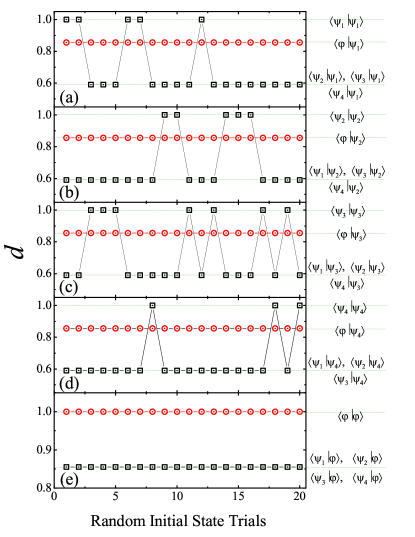
Figure 2: (Color online) Groundstate quantum FLS $d$ for the $4$-state Potts model as a function of random initial state trials. The reference states are chosen in (a) $|\Psi_{1}\rangle$, (b) $|\Psi_{2}\rangle$, (c) $|\Psi_{3}\rangle$, (d) $|\Psi_{4}\rangle$, and (e) $|\varphi\rangle$. It is clearly shown that, if the reference state is chosen as one of the degenerate groundstates in the broken symmetry phase, the other three groundstates has the same value of the FLS in (a)-(d). If the reference state is chosen as the groundstate in the symmetry phase, the FLSs for the four degenerate groundstates has the same value in the broken symmetry phase in (e).

In order to show clearly how to detect degenerate groundstates based on Eq. (5), as an example, we consider the $4$-state Potts model. In Fig. 1, we plot the FLS $d$ for random initial states. Here, $\lambda=0.8$ and $1.2$ are chosen. Due to the broken $Z_{4}$ symmetry for $q=4$, the system has $4$ degenerate groundstats for the broken symmetry phase $\lambda<\lambda_{c}=1$. It is clearly shown that, for $\lambda=0.8$ $(\lambda<\lambda_{c})$, there exist four different values of the FLS, while, for $\lambda=1.2$ $(\lambda>\lambda_{c})$, there exists only one value of the FLS. From each value of the FLS for $\lambda=0.8$, we label the four degenerate groundstates as $|\psi_{1}\rangle$, $|\psi_{2}\rangle$, $|\psi_{3}\rangle$, and $|\psi_{4}\rangle$. For for $\lambda=1.2$, the groundstate is denoted by $|\varphi\rangle$. Actually, we have chosen more than 200 random initial states. The probability $P(n)$, that the system is in each groundstate for $\lambda<\lambda_{c}$, is found to be $P(n)\simeq 1/4$ in the broken symmetry phase. Then, for the $q$-state Potts model, with a large number of random initial state trials, one may detect the $q$ degenerate groundstates with the probability $P(n\rightarrow\infty)=1/q$ finding each degenerate groundstate in the broken $Z_{q}$ symmetry phase.

One may choose the reference state as one of the degenerate groundstates. In Fig. 2, we choose the reference state as one of the groundstates for the broken symmetry phase in (a) $|\Psi_{1}\rangle$, (b) $|\Psi_{2}\rangle$, (c) $|\Psi_{3}\rangle$, and (d) $|\Psi_{4}\rangle$, and as the groundstate $|\varphi\rangle$ for the symmetry phase in (e). In Figs. 2(a)-(d), it is clearly shown that, for $\lambda=0.8$ $(\lambda<\lambda_{c})$, there exist two different values of the FLS, i.e., $d(|\psi_{m}\rangle,|\psi_{m}\rangle)=1$ and $d(|\psi_{m}\rangle,|\psi_{m\neq m^{\prime}}\rangle)=constant\neq 1$ $(m,m^{\prime}\in[1,q])$. Furthermore, $d(|\psi_{m}\rangle,|\varphi\rangle)=constant$. In Fig. 2 (e), the reference state chosen as the groundstate in the symmetry phase shows $d(|\varphi\rangle,|\varphi\rangle)=1$ and $d(|\psi_{m}\rangle,|\varphi\rangle)=constant\neq 1$. In this case, as discussed in Ref. Dai, , one may use a probability mass distribution function, as an alternative way, to distinguish the degenerate groundstates. Here, it is shown that the degenerate states can be distinguished by a reference state chosen as arbitrary states except for the degenerate groundstates in the broken symmetry phase and the groundstate in the symmetry phase.

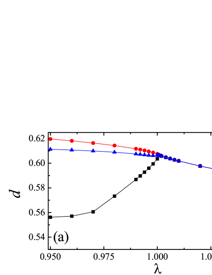
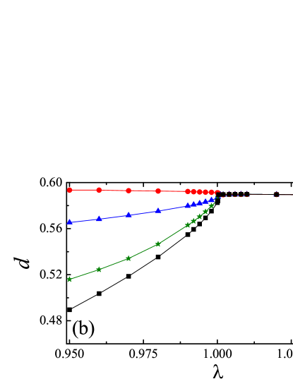
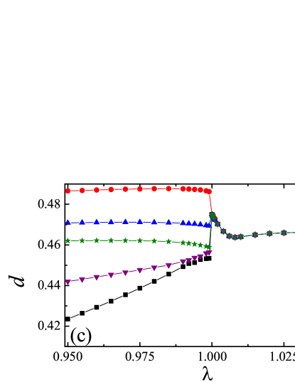
Figure 3: (Color online) Groundstate quantum FLS $d$ for (a) $3$-, (b) $4$-, and (c) $5$-state Potts models as a function of the transverse magnetic field $\lambda$ with the truncation dimension $\chi=32$. In the broken symmetry phase, the $q$ branches of the FLS correspond to the numbers of the $q$ degenerate groundstates. As the magnetic field crosses the critical point $\lambda_{c}$, the FLSs show the multiple bifurcations with three, four, and five branches, respectively, in the broken symmetry phase. Note that, for the $3$- and $4$-state Potts models, the FLSs show their continues behaviors, while, for the $5$-state Potts model, the FLS shows a discontinues behavior. These continues and discontinues behaviors indicate the continues phase transitions for $q=3$ and $4$, and the discontinues phase transition for $q=5$. The numerical multiple bifurcations are given as $\lambda_{c}=1.0004$ for $q=3$ and $4$ and $\lambda_{c}=1$ for $q=5$.

V Quantum Fidelity per lattice site for phase transitions

In the view of a groundstate degeneracy, the degenerate groundstates in the broken symmetry phase exist until the system reaches its critical point. Once one can detect degenerate groundstates, one may also detect a quantum phase transition by the quantum fidelity in Eq. (5). Detected degenerate groundstate wavefunctions may allow us also to investigate directly a property of quantum phases even for unexplored broken symmetry phases. In this section, then, we will discuss the quantum phase transitions for the $q$-state Potts model. In the next section, we will discuss the relation between system symmetry and order parameter directly from groundstates.

From the detected degenerate groundstates, in Fig. 3, we plot the FLSs as a function of the transverse magnetic field $\lambda$ for $q=3$, $4$, and $5$. Here, the truncation dimension is chosen as $\chi=32$. Figure 3 shows clearly that, as the transverse magnetic field decreases, the FLSs in the symmetry phase branch off the $q$ FLSs. The branch points are estimated numerically as $\lambda_{c}=1.0004$ for the $3$- and $4$-state Potts models. Also, for the $5$-state Potts model, the multiple bifurcation point exists exactly at $\lambda_{c}=1$. These results show that the branch points agree well the exact critical point $\lambda_{c}=1$. Then, the branch points correspond to the critical point. Such a branching behavior of the FLS can be called as multiple bifurcation and a branch point as multiple bifurcation point. Consequently, it is shown that the FLS from the quantum fidelity between degenerate groundstates and a reference state can detect a quantum phase transition.

As is known, for the $q$-state Potts model, the continues (discontinuous) phase transitions occurs for $q\leq 4$ ($q>4$). Figs. 3 (a) for $q=3$ and (b) $q=4$ show that the FLSs are a continues function for the quantum phase transition. While Fig. 3 (c) $q=5$ shows that the FLS is a discontinues function for the quantum phase transition. Then, the continues (discontinues) behaviors at the critical points imply that a continues (discontinues) phase transition occurs. As a result, the FLS in Eq. (5) can clarify continues (discontinues) quantum phase transitions.

VI Symmetry and order parameter

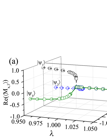
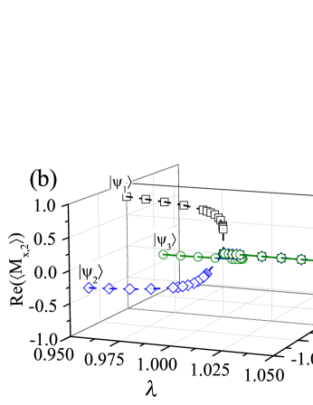
Figure 4: (Color online) Magnetization (a) $\langle M_{x,1}\rangle$ and (b) $\langle M_{x,2}\rangle$ as a function of the transverse magnetic field $\lambda$ for the 3-state Potts model. For the broken symmetry phase $\lambda<\lambda_{c}$, each magnetization is given for each of the three degenerate groundstates denoted by $|\psi_{m}\rangle$ $(m\in[1,q]$. The numerical critical point locates at $\lambda_{c}=1.0004$.

The existence of a degenerate groundstate means that each of degenerate groundstates possess its own order described by each corresponding order parameter. The each order parameter, which is nonzero value only in an ordered phase, should distinguish an ordered phase from disordered phasesMichel . To complete the description of an ordered phase, it is required to specify how each order parameter from each of degenerate groundstates transforms under a symmetry group $G$ that is possessed by the Hamiltonian because each order parameter is invariant under only a subgroup of the symmetry group $G$ although the Hamiltonian remains invariant under the full symmetry group $G$  Chaikin . Then, in this section, we discuss local magnetizations obtained from each of the degenerate groundstates.

Let us first discuss the local magnetizations for the $3$-state Potts model, i.e., $q=3$. In Fig. 4, we plot the magnetization (a) $\langle M_{x,1}\rangle$ and (b) $\langle M_{x,2}\rangle$ as a function of the traverse magnetic field $\lambda$. The magnetizations disappear to zero at the numerical critical point $\lambda_{c}=1.0004$. Also, all the magnetizations show that the phase transition is a continuous phase transition. For the broken symmetry phase $\lambda<\lambda_{c}$, each magnetization is calculated from each of the three degenerate groundstates, which is denoted by $|\psi_{m}\rangle$. Note that all the absolute values of the magnetizations $\langle\psi_{m}|M_{x,p}|\psi_{m}\rangle\equiv\langle M_{x,p}\rangle_{m}$ are the same values at a given magnetic field. Furthermore, for a given magnetic field, the magnetizations in the complex magnetization plane seem to have a relation between them under a rotation, which is characterized by the value $\omega_{3}=\exp[2\pi i/3]$. Then, in Figs. 4(a) and (b), it is observed that, for a given magnetic field $\lambda<\lambda_{c}$, there are the relations between the magnetizations as $\langle M_{x,1}\rangle_{1}=\omega^{-1}_{3}\langle M_{x,1}\rangle_{2}=\omega^{-2}_{3}\langle M_{x,1}\rangle_{3}$ and $\langle M_{x,2}\rangle_{1}=\omega^{-2}_{3}\langle M_{x,2}\rangle_{2}=\omega^{-4}_{3}\langle M_{x,2}\rangle_{3}$. Also, for each groundstate wavefunction, the magnetizations have the relations as $\langle M_{x,1}\rangle_{1}=\langle M_{x,2}\rangle_{1}$, $\langle M_{x,1}\rangle_{2}=\omega^{-1}_{3}\langle M_{x,2}\rangle_{2}$, and $\langle M_{x,1}\rangle_{3}=\omega^{-2}_{3}\langle M_{x,2}\rangle_{3}$. These results show that, in the complex magnetization plane, the rotations between the magnetizations for a given magnetic field are determined by the characteristic rotation angles $\theta=0$, $2\pi/3$, and $4\pi/3$, i.e., $\langle M_{x,p}\rangle_{m}=g_{3}\langle M_{x,p^{\prime}}\rangle_{m^{\prime}}$ with $g_{3}\in\{I,\omega_{3},\omega^{2}_{3}\}$. Here, we have chosen the $|\psi_{1}\rangle$ that gives a real value of the magnetizations, i.e., $\langle M_{x,1}\rangle_{1}$ and $\langle M_{x,2}\rangle_{1}$ are real. Also, the degenerate groundstates give the same values for the $z$-component magnetizations, i.e., $\langle M_{z}\rangle_{1}=\langle M_{z}\rangle_{2}=\langle M_{z}\rangle_{3}$.

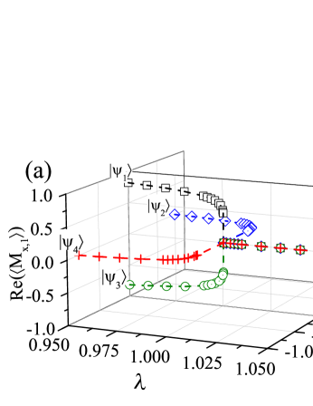
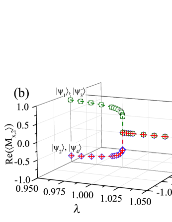
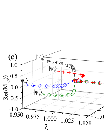
Figure 5: (Color online) Magnetizations (a) $\langle M_{x,1}\rangle$, (b) $\langle M_{x,2}\rangle$, and (c) $\langle M_{x,3}\rangle$ as a function of the transverse magnetic field $\lambda$ for the $4$-state Potts model. For the broken symmetry phase, the magnetizations are given from each of the four degenerate groundstates. The critical point is estimated numerically as $\lambda_{c}=1.0004$.

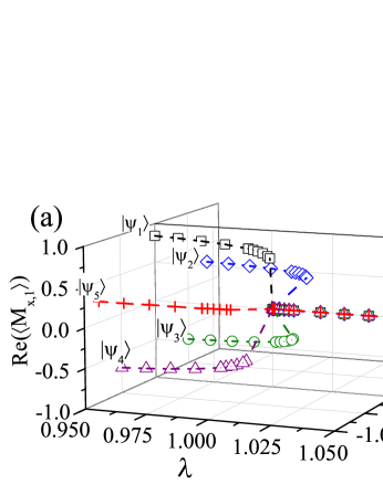
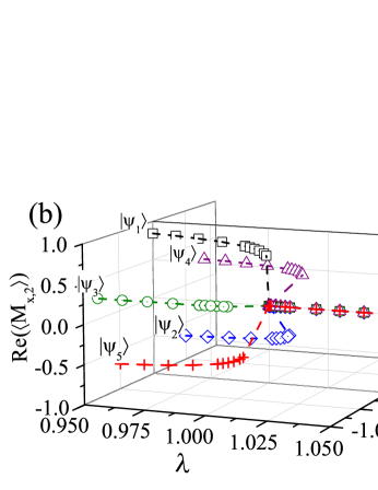
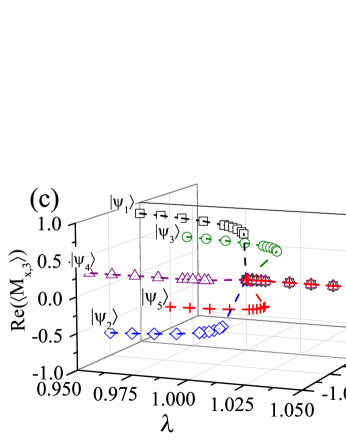
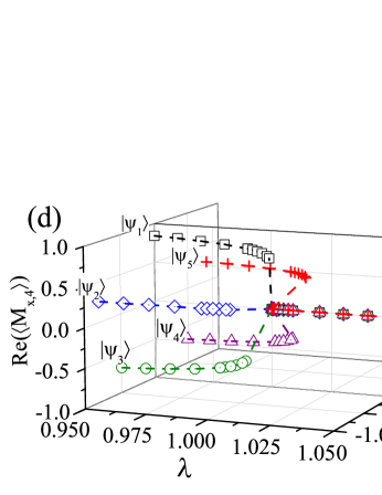
Figure 6: (Color online) Magnetizations (a) $\langle M_{x,1}\rangle$, (b) $\langle M_{x,2}\rangle$, (c) $\langle M_{x,3}\rangle$, and (d) $\langle M_{x,4}\rangle$ as a function of the transverse magnetic field $\lambda$ for the $5$-state Potts model. For the broken symmetry phase, the magnetizations are given from each of the five degenerate groundstates. The numerical critical point is the exact value $\lambda_{c}=1$.

Next, we consider the magnetizations for the $4$-state Potts model, i.e., $q=4$. In Fig. 5, we plot the magnetization (a) $\langle M_{x,1}\rangle$, (b) $\langle M_{x,2}\rangle$, and (c) $\langle M_{x,3}\rangle$ as a function of the traverse magnetic field $\lambda$. The numerical critical point is $\lambda_{c}=1.0004$. All the magnetizations show that the phase transition is a continuous phase transition. Similar to the case $q=3$, all the absolute values of the magnetizations have the same values at a given magnetic field and the magnetizations in the complex magnetization plane have a relation between them under a rotation, which is characterized by the value $\omega_{4}=\exp[2\pi i/4]$. In Fig. 5, we observe that, for a given magnetic field $\lambda<\lambda_{c}$, there are the relations between the magnetizations as $\langle M_{x,1}\rangle_{1}=\omega^{-1}_{4}\langle M_{x,1}\rangle_{2}=\omega^{-2}_{4}\langle M_{x,1}\rangle_{3}=\omega^{-3}_{4}\langle M_{x,1}\rangle_{4}$ from (a), $\langle M_{x,2}\rangle_{1}=\omega^{-2}_{4}\langle M_{x,2}\rangle_{2}=\omega^{-4}_{4}\langle M_{x,2}\rangle_{3}=\omega^{-6}_{4}\langle M_{x,2}\rangle_{4}$ from (b), and $\langle M_{x,3}\rangle_{1}=\omega^{-3}_{4}\langle M_{x,3}\rangle_{2}=\omega^{-6}_{4}\langle M_{x,3}\rangle_{3}=\omega^{-9}_{4}\langle M_{x,3}\rangle_{4}$ from (c). Also, for each groundstate wavefunction, the magnetizations have the relations as $\langle M_{x,1}\rangle_{1}=\langle M_{x,2}\rangle_{1}=\langle M_{x,3}\rangle_{1}$, $\langle M_{x,1}\rangle_{2}=\omega^{-1}_{4}\langle M_{x,2}\rangle_{2}=\omega^{-2}_{4}\langle M_{x,3}\rangle_{2}$, $\langle M_{x,1}\rangle_{3}=\omega^{-2}_{4}\langle M_{x,2}\rangle_{3}=\omega^{-4}_{4}\langle M_{x,3}\rangle_{3}$, and $\langle M_{x,1}\rangle_{4}=\omega^{-3}_{4}\langle M_{x,2}\rangle_{4}=\omega^{-6}_{4}\langle M_{x,3}\rangle_{4}$. These results show that, in the complex magnetization plane, the rotations between the magnetizations for a given magnetic field are determined by the characteristic rotation angles $\theta=0$, $2\pi/4$, $4\pi/4$, and $6\pi/4$, i.e., $\langle M_{x,p}\rangle_{m}=g_{4}\langle M_{x,p^{\prime}}\rangle_{m^{\prime}}$ with $g_{4}\in\{I,\omega_{4},\omega^{2}_{4},\omega^{3}_{4}\}$. Also, the degenerate groundstates give the same values for the $z$-component magnetizations, i.e., $\langle M_{z}\rangle_{1}=\langle M_{z}\rangle_{2}=\langle M_{z}\rangle_{3}=\langle M_{z}\rangle_{4}$.

From the discussions for the $3$-state and $4$-state Potts models, one may refer a general relation between the magnetizations for any $q$-state Potts model. Actually, for any $q$, we find the relations

$$\omega^{p(1-m)}_{q}\langle M_{x,p}\rangle_{m} = \omega^{p^{\prime}(1-m^{\prime})}_{q}\langle M_{x,p^{\prime}}\rangle_{m^{\prime}},$$ (6a)

$$\langle M_{z}\rangle_{m} = \langle M_{z}\rangle_{m^{\prime}},$$ (6b)

where $\omega_{q}=\exp[2\pi i/q]$. When one calculate the magnetizations of the operator $M_{x,p}$ with different wavefunctions, the relations in Eq. (6) reduce to $\langle M_{x,p}\rangle_{m}=\omega^{p(m-m^{\prime})}_{q}\langle M_{x,p}\rangle_{m^{\prime}}$ that satisfies the relations of the magnetizations in Figs. 4 and 5. Also, if one choose a wavefunction, the magnetizations of the operators $M_{x,1}$, $\cdots$, $M_{x,q-2}$, and $M_{x,q-1}$ have the relations $\langle M_{x,p}\rangle_{m}=\omega^{(p^{\prime}-p)(1-m)}_{q}\langle M_{x,p^{\prime}}\rangle_{m}$ reduced from the relations in Eq. (6). Furthermore, these results show that, in the complex magnetization plane, the rotations between the magnetizations for a given magnetic field are determined by the characteristic rotation angles $\theta=0$, $2\pi/q$, $4\pi/q$, $6\pi/q$, $\cdots$, and $2(q-1)\pi/q$. Thus, Eq. (6) can be rewritten as

$$\langle M_{x,p}\rangle_{m} = g_{q}\langle M_{x,p^{\prime}}\rangle_{m^{\prime}},$$ (7a)

$$g_{q} \in \{I,\omega_{q},\omega^{2}_{q},\cdots,\omega^{q-1}_{q}\}.$$ (7b)

Then, Eq. (7) shows clearly that the $q$-state Potts model has the discrete symmetry group $Z_{q}$ consisting of $q$ elements. For $q=2$, the $q$-state Potts model becomes the quantum Ising model that has a doubly degenerate groundstate due to a $Z_{2}$ symmetry. From Eq. (7), one can easily confirm $\langle M_{x}\rangle_{1}=-\langle M_{x}\rangle_{2}$ because of $g_{2}\in\{I,\omega_{2}\}$ with $\omega_{2}=\exp[\pi i]$. Also, the $q$-state Potts Hamiltonian in Eq. (4) is invariant with respect to the $q$ way transformations, i.e., $U_{m}H_{q}U^{\dagger}_{m}=H_{q}$ for $m\in[1,q]$, which implies that the system has the $q$-fold degenerate groundstates for the broken symmetry phase according to the spontaneous symmetry breaking mechanism. The transformations are given as

$$U_{m}:\left\{\begin{array}[]{ccc}M_{x,p}&\rightarrow&\big{(}\omega^{p}_{q}\big{)}^{m-1}M_{x,p}\\ M_{z}&\rightarrow&M_{z}\end{array}\right.,$$ (8)

where $\omega_{q}=\exp[2\pi i/q]$. Although the $q$-state Potts Hamiltonian remains invariant under the full $q$ transformations, for the $Z_{q}$ broken symmetry phase, the $q$ order states described by the $q$ degenerate groundstates are invariant under only the subgroup of the $Z_{q}$ symmetry group. Obviously, Eqs. (6) and (7) show the relations between the order parameters of the $q$ equivalent ordered states under the $q$ transformations. As a consequence, it is shown that, from the degenerate groundstates, one can determine the order parameters as the magnetizations and their specification of how the order parameters transform under the symmetry group $Z_{q}$.

To make clearer the general relation of the magnetizations in Eqs. (6) and (7), let us consider the $5$-state Potts model. In Fig. 6, we plot the magnetization (a) $\langle M_{x,1}\rangle$, (b) $\langle M_{x,2}\rangle$, (c) $\langle M_{x,3}\rangle$, and (d) $\langle M_{x,4}\rangle$ as a function of the traverse magnetic field $\lambda$. The numerical critical point is obtained as the exact value $\lambda_{c}=1$. Also, all the magnetizations shows that the phase transition is a discontinues phase transition. Similar to the cases $q=3$ and $q=4$, all the magnetizations have the same values at a given magnetic field. and the magnetizations in the complex magnetization plane have a relation between them under a rotation, which is characterized by the value $\omega_{5}=\exp[2\pi i/5]$. From Figs. 6 (a)-(d), the relations between the magnetizations agree with those in Eqs. (6) and (7).

VII Critical exponents, Central charge, and universality

Table 1: Critical exponents and central charge for $4$-state Potts model

${\rm Exponents}$	$\alpha$	$\beta$	$\gamma$	$\delta$	$\nu$	$\eta$	$c$
${\rm Exact}$	$2/3$	$1/12$	$7/6$	$15$	$2/3$	$1/4$	$1$
${\rm iMPS}$		$0.0843$	$1.0718$		$0.6300$	$0.2510$	$0.9803$

As is known, for $q\leq 4$, the quantum phase transitions are a continuous phase transition. If $q>4$, discontinuous (first order) phase transitions occur in the $q$-state Potts model. In this sense, then, the critical $q$ is $q_{c}=4$. In the section, we will study the critical exponents of $q_{c}=4$ based on the iMPS groundstate wavefunctions. Actually, all the degenerate groundstates for the broken symmetry phase give a same exponents as it should be. In addition, in order to calculate a central charge, we discuss the von Neumann entropy for $q=3$, $4$, and $5$. In the Table 1, for the $4$-state Potts model, the critical exponents and the critical charge from the our iMPS results are compared with their exact values.

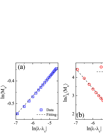
Figure 7: (Color online) (a) Magnetization $\langle M_{x}\rangle$ and (b) susceptibility $\partial_{\lambda}\langle M_{x}\rangle$ as a function of $|\lambda-\lambda_{c}|$ near the critical point $\lambda_{c}=1.0004$ for $4$-state Potts model.

Critical exponents.$-$ In our iMPS approach, we obtain the $4$-fold degenerate groundstates at zero temperature. The critical exponents $\alpha$ for specific heat and $\delta$ for the field dependence of the magnetization at the critical temperature cannot be calculated. In the following, we discuss the four exponents, i.e., $\beta$, $\gamma$, $\eta$, and $\nu$. Thus, we start with the magnetization near the critical point $\lambda_{c}=1.0004$. In Fig. 7, (a) the magnetization $\langle M_{x}\rangle$ and (b) the susceptibility $\partial_{\lambda}\langle M_{x}\rangle$ are plotted as a function of $|\lambda-\lambda_{c}|$ in the log-log plot. It is shown clearly that both the magnetization and the susceptibility can be described by power laws, i.e., $\langle M_{x}\rangle\propto|\lambda-\lambda_{c}|^{\beta}$ and $\partial_{\lambda}\langle M_{x}\rangle\propto|\lambda-\lambda_{c}|^{-\gamma}$ with their characteristic exponents $\beta$ and $\gamma$, respectively. Thus, the fitting function is chosen to be $\ln\langle M_{x}\rangle=\beta\ln|\lambda-\lambda_{c}|+\beta_{0}$ for the magnetization and $\ln\partial_{\lambda}\langle M_{x}\rangle=-\gamma\ln|\lambda-\lambda_{c}|+\gamma_{0}$ for the susceptibility with the fitting constants $\beta_{0}$ and $\gamma_{0}$, respectively. From the numerical fittings, we obtain (a) $\beta=0.0843$ and $\beta_{0}=0.0394$ for the magnetization and (b) $\gamma=1.0718$ and $\gamma_{0}=-3.0308$ for the susceptibility. The fitted critical exponents $\beta=0.0843$ and $\gamma=1.0718$ are quite close to the exact valuesWu $\beta=1/12\ (=0.0833)$ and $\gamma=7/6\ (=1.1667)$, respectively.

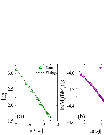
Figure 8: (Color online) (a) Correlation length $\xi$ as a function of $|\lambda-\lambda_{c}|$ for the $4$-state Potts model. (b) Correlation $\langle M_{x}(i)M_{x}(j)\rangle$ as a function of the lattice site distance $|i-j|$ at the critical point $\lambda_{c}=1.0004$.

In Fig. 8, we plot (a) the correlation length $\xi$ as a function of $|\lambda-\lambda_{c}|$ and (b) the correlation $\langle M_{x}(i)M_{x}(j)\rangle$ as a function of the lattice site distance $|i-j|$ at the critical point $\lambda_{c}=1.0004$. It is shown clearly that both the correlation length and the correlation at the critical point $\lambda_{c}$ can be described by power laws, i.e., $\xi\propto|\lambda-\lambda_{c}|^{-\nu}$ and $\langle M_{x}(i)M_{x}(j)\rangle\propto|\lambda-\lambda_{c}|^{-\eta}$ with their characteristic exponents $\nu$ and $\eta$, respectively. We choose the fitting functions as $\ln\xi=-\nu\ln|\lambda-\lambda_{c}|+\nu_{0}$ for the correlation length and $\ln\langle M_{x}(i)M_{x}(j)\rangle=-\eta\ln|i-j|+\eta_{0}$ for the correlation at the critical point with the fitting constants $\nu_{0}$ and $\eta_{0}$, respectively. From the numerical fittings, we obtain (a) $\nu=0.6300$ and $\nu_{0}=-1.2153$ for the correlation length and (b) $\eta=0.2510$ and $\eta_{0}=-3.5644$ for the correlation. The fitted critical exponents $\nu=0.6300$ and $\eta=0.2510$ are quite close to the exact valuesWu $\nu=2/3$ and $\eta=1/4$, respectively.

von Neumann entropy and central charge.$-$ In our iMPS approach, the von Neumann entropy $S$ can be directly evaluated by the elements of the diagonal matrix $\lambda^{[i]}_{\alpha_{i}}$ that are the Schmidt decomposition coefficients of the bipartition between the semi-infinite chains $L(-\infty,...,i)$ and $R(i+1,...,\infty)$. This implies that Eq. (1) can be rewritten by $|\Psi\rangle=\sum^{\chi}_{\alpha=1}\lambda_{\alpha}|\psi^{L}_{\alpha}\rangle|\psi^{R}_{\alpha}\rangle$, where $|\psi^{L}_{\alpha}\rangle$ and $|\psi^{R}_{\alpha}\rangle$ are the Schmidt bases for the semi-infinite chains $L(-\infty,...,i)$ and $R(i+1,...,\infty)$, respectively. For the bipartition, then, the von Neumann entropy $S$ can be defined as Bennett $S=-{\rm Tr}[\varrho_{L}\log\varrho_{L}]=-{\rm Tr}[\varrho_{R}\log\varrho_{R}]$, where $\varrho_{L}={\rm Tr}_{R}\,\varrho$ and $\varrho_{R}={\rm Tr}_{L}\,\varrho$ are the reduced density matrices of the subsystems $L$ and $R$, respectively, with the density matrix $\varrho=|\Psi\rangle\langle\Psi|$. For the semi-infinite chains $L$ and $R$ in the iMPS representation, the von Neumann entropy $S$ calculated by $S=-\sum_{\alpha=1}^{\chi}\lambda^{2}_{\alpha}\log\lambda^{2}_{\alpha}$. Actually, the von Neumann entropy as one of the quantum entanglement measures have been proposed as a general indicator to determine and characterize quantum phase transitionsKorepin ; entropy . Also, the logarithmic scaling of the von Neumann entropy was conformed to exhibit conformal invariance and the scaling is governed by a universal factorTagliacozzo ; Pollmann ; Zanardi , i.e., a central charge $c$ of the associated conformal field theory. In the iMPS approach, for a continuous phase transition, the diverging entanglement at a quantum critical point gives simple scaling relationsTagliacozzo for (i) the von Neumann entropy $S$ and (ii) a correlation length $\xi_{v}$ with respect to the truncation dimension $\chi$ as $S\sim\frac{c\kappa}{6}\log\chi$ and $\xi_{v}\sim A\chi^{\,\kappa}$, where $c$ is a central charge, $\kappa$ is a so-called finite-entanglement scaling exponent, and $A$ is a constant. By using the relations, a central charge can be obtained numerically at a critical point.

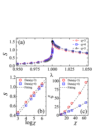
Figure 9: (Color online) (a) Groundstate von Neumann entropies for the $3$-, $4$-, and $5$-state Potts models as a function of the transverse magnetic field $\lambda$. (b) Von Neumann entropies $S$ and (c) Correlation lengthes $\xi_{v}$ for $q=3$ and $q=4$ with respect to the truncation dimension $\chi$ at the exact critical point $\lambda_{c}=1$.

In Fig. 9 (a), we plot the von Neumann entropies as a function of the transverse magnetic field $\lambda$ for the $3$-, $4$-, and $5$-state Potts models with the truncation dimension $\chi=32$. In the entropies, there are singular points at $\lambda_{c}=1.0004$ for $q=3$ and $4$, and $\lambda_{c}=1$ for $q=5$, which are consistent with the critical points from the multiple bifurcation points in Fig. 3 and from the magnetizations as the order parameters in Figs. 4, 5, and 6. It is shown clearly that the von Neumann entropies capture the phase transitions. The (dis-)continuity of the von Neumann entropies for $q=3$ and $q=4$ ($q=5$) indicates a (dis-)continuous phase transition between the broken symmetry phases and the symmetry phases. However, the von Neumann entropies for the different degenerate groundstates give the same values, which implies that the von Neumann entropy cannot distinguish the different degenerate groundstates in the broken symmetry phases.

For $q=3$ and $q=4$, in Figs. 9 (b) and (c), we plot (b) the von Neumann entropy and (c) the correlation length $\xi_{v}$ as a function of the truncation dimension $\chi$ at the critical points $\lambda_{c}=1$. Here, the truncation dimensions are taken as $\chi=8$, $16$, $25$, $32$, $50$, and $64$. It is shown that both the von Neumann entropy $S$ and the correlation length $\xi_{v}$ diverge as the truncation dimension $\chi$ increases. In order to obtain the central charges, we use the numerical fitting functions, i.e., $S_{q}(\chi)=a_{q}+b_{q}\log\chi$ and $\xi_{v,q}(\chi)=A_{q}\chi^{\,\kappa_{q}}$. Numerically, the constants of the von Neumann entropies are fitted as $a_{3}=-0.1215$ and $b_{3}=0.2000$ for $q=3$ and $a_{4}=-0.1830$ and $b_{4}=0.2016$ for $q=4$. The power-law fittings on the correlation lengthes $\xi_{v,q}$ give the fitting constants as $A_{3}=0.2060$ and $\kappa_{3}=1.4775$ for $q=3$. and $A_{4}=0.2243$ and $\kappa_{4}=1.2340$ for $q=4$. As a result, from the $\kappa_{q}$ and $b_{q}$, the central charges are obtained as $c_{3}=0.8121$ for $q=3$ and $c_{4}=0.9803$ for $q=4$, which are quite close to the exact valuesBaillie $c=4/5$ for $q=3$ and $c=1$ for $q=4$, respectively.

VIII Summary

We have investigated how to obtain degenerate groundstates by using a quantum fidelity. To do this, we have introduced the quantum fidelity between the degenerate groundstates and an arbitrary reference state. The distinguished degenerate groundstate wavefunctions allows naturally to detect a quantum phase transition that is indicated by a multiple bifurcation point of the quantum fidelity per lattice site. Furthermore, as the complete description of an order phase, it is possible to classify how the order parameters calculated from the degenerate groundstates transform under the subgroup of a symmetry group of Hamiltonian. As an example, the $q$-state Potts model has been investigated by employing the iMPS with the iTEBD. We have obtained the $q$-fold degenerated groundstates explicitly. A general relation between the magnetizations calculated from the degenerate groundstates is obtained to show the spontaneous symmetry breaking of the $Z_{q}$ symmetry group in the $q$-state Potts model. In addition, the critical exponents and the central charges are directly calculated from the degenerate groundstates, which is shown that the iMPS results are quite close to the exact values.

References

- (1) S. Sachdev, Quantum Phase Transitions (Cambridge University, Cambridge, 1999).
- (2) P. M. Chaikin and T. C. Lubensky, Pinciples of Condensed Matter Physics (Cambridge University, Cambridge, 1995).
- (3) L. D. Landau and E. M. Lifshitz, Statistical Physics (Pergamon, New York, 1958).
- (4) H.-Q. Zhou and J. P. Barjaktarevič, J. Phys. A: Math. Theor. 41, 412001 (2008); H.-Q. Zhou, J.-H. Zhao, and B. Li, J. Phys. A: Math. Theor. 41, 492002 (2008).
- (5) P. Zanardi and N. Paunković, Phys. Rev. E 74, 031123 (2006).
- (6) M. M. Rams and B. Damski, Phys. Rev. Lett. 106, 055701 (2011).
- (7) V. Mukherjee and A. Dutta, Phys. Rev. B 83, 214302 (2011).
- (8) H.-Q. Zhou, arXiv:0704.2945; E. Eriksson and H. Johannesson, Phys. Rev. A 79, 060301(R) (2009); Z. Wang, T. Ma, S.-J. Gu, and H.-Q. Lin, Phys. Rev. A 81, 062350 (2010); J.-H. Liu, Q.-Q. Shi, J.-H. Zhao, and H.-Q. Zhou, J. Phys. A: Math. Theor. 44, 495302 (2011).
- (9) S.-J. Gu, Int. J. Mod. Phys. B 24, 4371 (2010).
- (10) X. Wang, Z. Sun, and Z. D. Wang, Phys. Rev. A 79, 012105 (2009).
- (11) H.-L. Wang, J.-H. Zhao, B. Li, and H.-Q. Zhou, J. Stat. Mech., L10001 (2011).
- (12) M. Fannes, B. Nachtergaele, and R. F. Werner, Comm. Math. Phys, 144, 3 (1994); S. Östlund and S. Rommer. Phys. Rev. Lett. 75, 3537 (1995); D. Perez-Garcia, F. Verstraete, M. M. Wolf, and J. I. Cirac, Quantum Inf. Comput. 7, 401 (2007).
- (13) S. R. White, Phys. Rev. Lett. 69, 2863 (1992); S. R. White, Phys. Rev. B. 48, 10345 (1993); U. Schollwöck, Rev. Mod. Phys. 77, 259 (2005).
- (14) G. Vidal, Phys. Rev. Lett. 91, 147902 (2003); G. Vidal, Phys. Rev. Lett. 98, 070201 (2007).
- (15) H.-Q. Zhou, Roman Orús, and G. Vidal, Phys. Rev. Lett. 100, 080601 (2008).
- (16) J.-H. Zhao, H.-L. Wang, B. Li, and H.-Q. Zhou, Phys. Rev. E 82, 061127 (2010).
- (17) S.-H. Li, H.-L. Wang, Q.-Q. Shi, and H.-Q. Zhou, arXiv:1105.3008; H.-L. Wang, Y.-W. Dai, B.-Q. Hu, and H.-Q. Zhou, Phys. Lett. A 375, 4045 (2011).
- (18) Y.-W. Dai, B.-Q. Hu, J.-H. Zhao, and H.-Q. Zhou, J. Phys. A: Math. Theor. 43, 372001 (2010).
- (19) R. B. Potts, Proc. Cambridge Phil. Soc. 48, 106 (1952).
- (20) F. Y. Wu, Rev. Mod. Phys. 54, 235 (1982); R. J. Baxter, Exactly Solved Models in Statistical Mechanics (Academic, London, 1982); P. P. Martin, Potts Models and Related Problems in Statistical Mechanics (World Scientific, Singapore, 1991).
- (21) V. Murg, F. Verstraete, and J. I. Cirac, Phys. Rev. A 75, 033605 (2007).
- (22) M. Suzuki, Phys. Lett. A 146, 319 (1990).
- (23) R. J. Baxter, J. Phys. C 6, L445 (1973); R. J. Baxter, J. Phys. A 15, 3329 (1982).
- (24) M. P. M. Nijs, J. Phys. A 12, 1857 (1979); M. P. M. Nijs, Phys. Rev. B 27, 1674 (1983).
- (25) R. B. Pearson, Phys. Rev. B 22, 2579 (1980).
- (26) J. Black and V. J. Emery, Phys. Rev. B 23, 429 (1981).
- (27) M. Caselle, F. Gliozzi and S. Necco, J. Phys. A: Math. Gen. 34, 351 (2001).
- (28) J. Hove, J. Phys. A 38, 10893 (2005).
- (29) L. Michel, Rev. Mod. Phys. 52, 617 (1980).
- (30) C. F. Baillie and D. A. Johnston, Mod. Phys. Lett. A 7, 1519 (1992).
- (31) C. H. Bennett, H. J. Bernstein, S. Popescu, and B. Schumacher, Phys. Rev. A 53, 2046 (1996).
- (32) V. E. Korepin, Phys. Rev. Lett. 92, 096402 (2004); P. Calabrese and J. Cardy, J. Stat. Mech.: Theory Exp., P06002 (2004).
- (33) L. Amico, R. Fazio, A. Osterloh, and V. Vedral, Rev. Mod. Phys. 80, 517 (2008).
- (34) L. Tagliacozzo, T. R. de Oliveira, S. Iblisdir, and J. I. Latorre, Phys. Rev. B 78, 024410 (2008).
- (35) F. Pollmann, S. Mukerjee, A. M. Turner, and J. E. Moore, Phys. Rev. Lett. 102, 255701 (2009).