A mathematical model of sap exudation in maple trees governed by ice melting, gas dissolution and osmosis.

Abstract

We develop a mathematical model for sap exudation in a maple tree that is based on a purely physical mechanism for internal pressure generation in trees in the leafless state. There has been a long-standing controversy in the tree physiology literature over precisely what mechanism drives sap exudation, and we aim to cast light on this issue. Our model is based on the work of Milburn and O’Malley [Can. J. Bot., 62(10):2101–2106, 1984] who hypothesized that elevated sap pressures derive from compressed gas that is trapped within certain wood cells and subsequently released when frozen sap thaws in the spring. We also incorporate the extension of Tyree [in Tree Sap, pp. 37–45, eds. M. Terazawa et al., Hokkaido Univ. Press, 1995] who argued that gas bubbles are prevented from dissolving because of osmotic pressure that derives from differences in sap sugar concentrations and the selective permeability of cell walls. We derive a system of differential-algebraic equations based on conservation principles that is used to test the validity of the Milburn–O’Malley hypothesis and also to determine the extent to which osmosis is required. This work represents the first attempt to derive a detailed mathematical model of sap exudation at the micro-scale.

1 Introduction

Sap flow in deciduous trees is driven during the growing season by the process of transpiration, in which evaporation of water in the leaves draws groundwater from the roots to the crown [14, 28]. As much as 90% of water taken up by the tree is transpired into the atmosphere to generate the large pressure differential needed to overcome gravity; only 10% of the water is actually consumed in photosynthesis reactions in the leaves to produce the sugars needed for growth and other life processes. These sugars are transported by the sap in dissolved form back to the trunk and roots where they are either consumed immediately or else stored as starch for later use. Transpiration halts in late fall when the leaves drop and the tree enters its winter dormant phase, which lasts until the spring thaw. At that time, the stored starch reserves are released and provide the energy needed to initiate budding and leaf growth before photosynthesis and transpiration can begin again.

In the sugar maple (Acer saccharum), a process known as sap exudation occurs in the time period between the dormant leafless phase and the active transpiration phase, when certain processes are triggered that build up positive sap pressure and convert stored starches into sugars. The stem pressure is large enough that when the tree is tapped, sap exudes naturally from the tap-hole. The mechanism that generates this internal pressure is unique to the sugar maple and a few other related species (black and red maple, birch, walnut, and butternut) whose sap sugar content is also significant although not typically as high as sugar maple. Raw maple sap typically contains 2 to 3% sugar by weight (primarily sucrose) and can be processed by repeated boiling to produce sweet syrup and other edible maple products.

The scientific study of sap exudation has a long history that has seen several competing hypotheses proposed for the mechanism that drives sap flow in spring. These hypotheses can be roughly divided into two classes: “vitalistic” models that require some intervention by living cells; and “physical” models that rely on passive, physical effects. Early in the 20th century, Wiegand’s experiments [32] showed that even though up to one-quarter of the total volume of sapwood or xylem is filled with gas, the expansion and contraction of this gas in response to temperature changes alone could still not account for the observed pressure changes. He concluded that some active process initiated by living cells must be responsible, a claim that was supported by the experiments of Johnson [7].

Later studies questioned this vitalistic hypothesis, for example Stevens and Eggert [23] who attributed the pressure generation in leafless maple trees to volume changes arising from freezing and thawing of sap. This hypothesis was further explored in subsequent years [20, 25], culminating in the ground-breaking paper of Milburn and O’Malley [12] who proposed that gas trapped in the xylem is compressed by growth of ice crystals and subsequent uptake of water when the tree freezes in fall; during the spring thaw, they argued that this compressed gas generates the pressures that drive exudation. This freeze/thaw hypothesis was later supported by experimental evidence [8, 13] showing that gas expansion due to thawing sap is the primary cause of exudation pressure; they also found no evidence to suggest that living cells play a significant role.

However, the Milburn–O’Malley model was unable to account for all observations, and so some authors [22, 26, 28] cast doubt on the ability of gas expansion alone to explain exudation, arguing that heightened pressures in the xylem will dissolve any gas bubbles within a few hours. Several studies [5, 6] suggested that osmotic pressure, generated by differences in sugar concentration across semi-permeable structures that separate various cells in the xylem, could play a significant supporting role in sap exudation. Most notably, Tyree proposed [26] that a combination of the freeze/thaw mechanism and osmosis is the key to maintaining stable gas bubbles in the xylem over observed exudation time scales.

This issue remains controversial and the current situation is perhaps best summed up by Améglio et al. who concluded that “no existing single model explains all of the xylem winter pressure data,” so that both vitalistic and physical effects must play a role [2].  The lack of a clear consensus in the tree physiology literature regarding the precise mechanisms driving sap exudation is compounded by the fact that no detailed mathematical model has yet been developed for the freeze/thaw mechanism, not to mention the other effects of osmosis and gas dissolution.

The aim of this paper is therefore to develop a mathematical model that captures the essential processes driving sap exudation. We begin in Section 2 by providing details of tree physiology, sap flow, and the Milburn–O’Malley and Tyree hypotheses for pressure generation, at the core of which is the special role played by two types of non-living xylem cells called vessels and fibers. In Section 3 we derive a system of differential equations governing the multiphase gas/liquid/ice system that incorporates the effects of thawing sap in the fibers, dissolving gas bubbles in the vessels, and the osmotic pressure pressure gradient between the two. Numerical simulations in Section 4 are used to validate the model and conclusions are drawn regarding the various mechanism for sap generation in Section 5.

2 Basic tree physiology and the Milburn–O’Malley hypothesis

We first provide some background information on tree structure and the hydraulics of sap flow that can be found in texts such as [14, 28]. We also describe the freeze/thaw model proposed by Milburn and O’Malley, and indicate how other mechanisms such as gas dissolution and osmotic pressure enter the picture.

The Milburn–O’Malley model is a purely physical one that operates at the cellular level and depends fundamentally on the structure of the non-living cells making up the xylem. As pictured in Figure 1(a), the xylem consists of long, hollow, roughly cylindrical cells of two types: fibers, that are the main structural members in the wood; and vessels, that have a larger radius and form the primary conduit for transmitting sap. An individual vessel can extend for up to tens of centimeters vertically through the xylem, and is subdivided into elements that are connected end-to-end via perforated plates to form a continuous hydraulic connection. Vessels are connected to each other via numerous pits or cavities that perforate the vessel walls. The fibers are in turn subdivided into two sub-classes: libriform fibers and tracheids. According to Cirelli et al. [5], the tracheid walls also contain pits through which they exchange sap with the vessels and hence integrating the tracheids into the water transport system of the tree. We will therefore ignore the tracheids, treating them as a part of the vessel network, and focus instead on the fibers.

In comparison with tracheids, the libriform fibers (or simply “fibers”) lack the pits that provide a direct hydraulic connection to the vessels and so they are often considered to play a primarily structural role. However, the recent experiments of Cirelli et al. [5] suggest that the fiber secondary wall has a measurable permeability to water. Other experiments show that under normal conditions, maple trees (and other species that exude sap in spring) are characterized by gas-filled fibers and water-filled vessels [14, 26]. This is in direct contrast with most other tree species whose fibers are completely filled with water. Hence, it is reasonable to suppose that the presence of gas in xylem fibers may be connected with the ability of maple trees to generate exudation pressure in the leafless state.

The mechanism proposed by Milburn and O’Malley [12], and discussed in complete detail in [26], can be summarized as follows:

• During late fall or early winter when the tree freezes, ice crystals form on the inner wall of the fibers and the growing ice layer compresses the gas trapped inside.

• In early spring when temperatures rise above freezing, ice crystals in the fiber melt and the pressure of the trapped gas drives the melted sap through the fiber walls into the vessel, hence leading to the elevated pressures observed during sap exudation. Tyree [25] estimates that this effect is responsible for a pressure increase of roughly 30–60 $\mathrm{kPa}$.

• Exudation pressure is enhanced by the gravitational potential of sap that was drawn into the crown during the previous fall, and once thawed is then free to fall toward the roots.

As mentioned before, this model can account for the initiation of exudation pressure but it cannot explain how pressures are sustained over periods longer than about 12 hours because gas bubbles will dissolve when pressurized. Tyree [26] explains how surface tension effects require that any gas bubble is at higher pressure than the surrounding fluid. As a result, Henry’s law necessitates that the concentration of dissolved gas in the region adjacent to the bubble is proportional to interfacial pressure. Since the gas concentration is highest there, dissolved gas diffuses away from the bubble and eventually causes the bubble to disappear.

One clue to identifying a mechanism that can sustain gas bubbles over longer time periods is provided by experiments that show maple trees exude sap only when sugar is present [8]. With this in mind, Tyree [26] proposed a modification of the Milburn–O’Malley mechanism in which osmotic pressures arising from differences in sucrose concentration could permit gas bubbles to remain stable. In particular, he suggested that the fiber secondary walls are selectively permeable, permitting water to pass through but not larger molecules like sucrose. Therefore, the ice layer that forms on the inner surface of the fibers in fall/winter is composed of pure water, which leads to an osmotic potential difference between the fibers and the vessels.

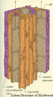
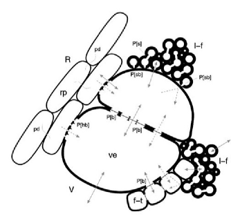
(a)  3D view of the xylem, showing vessel elements surrounded by fibers and illustrating the difference in the cell diameters. The pits forming the hydraulic connections between the cells are also shown. Source: [29].		(b)  2D cross-section highlighting the vessel elements ( ve), libriform fibers ( l-f), and fiber tracheids ( f-t). Source: Cirelli et al. [5, Fig. 6b] (reproduced with permission, Oxford Univ. Press).

Fig. 1: Two views of the layout of vessels and fibers in the xylem.

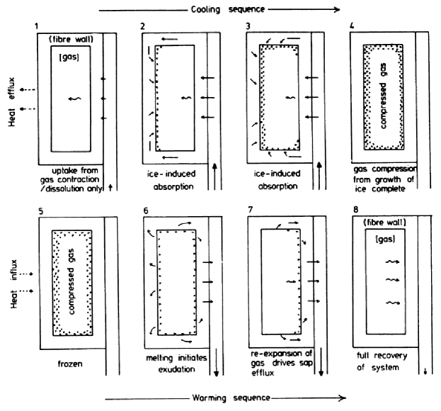
Fig. 2: Picture of ice and compressed gas taken from Milburn and O’Malley [12, Fig. 7] (© 2008 Canadian Science Publishing, reproduced with permission). We are concerned here only with the “warming sequence” in the bottom row, numbered 5–8. The fiber is the rectangular structure on the left of each image, while the vessel is represented by the vertical channel on the right (not drawn to scale).

3 Derivation of the model equations

We now derive a compartment model describing the dynamics of gas, water and ice in a single vessel that is in contact with the surrounding fibers. To begin with, we restrict ourselves to the time period before the ice in the fiber melts completely. The geometry is depicted in Figure 3 which is an idealized view of Figure 1(b). Before deriving the governing equations, we make the following simplifying assumptions:

1. We consider only the thawing phase, assuming that all water within the fibers is initially frozen.

2. Gravitational potential differences due to height can be neglected since we focus only locally on a small section of the xylem.

3. We consider a single vessel element and ignore interactions between adjacent elements. This is a reasonable assumption if all elements experience similar conditions, and any gas contained within an element is isolated by the perforated plates from that of its neighbors.

4. The vessel is surrounded by $N$ identical fibers. Although our model considers only a single fiber explicitly, the fluxes and other fiber quantities are scaled by a factor $N$ to determine the total influence of all $N$ fibers on the vessel.

5. The fiber and vessel are hollow and cylindrical in shape, with interior radii $R^{f}$ and $R^{v}$, and heights $0pt^{f}$ and $0pt^{v}$ respectively. Both have large aspect ratio so that $R/0pt\ll 1$.

6. We assume the problem is one-dimensional, with the domain extending horizontally from the center of the fiber to the rightmost outer edge of the vessel (pictured at the top of Figure 3). The coordinate system is chosen so that the horizontal ($x$) axis is directed along the line joining the centers of the fiber and vessel and with origin $x=0$ at the center of the fiber. Referring to Figure 3, the fiber/vessel interface is located at $x=R^{f}$ and the center of the vessel at $x=R^{f}+R^{v}$.

7. Gas is present in both fiber and vessel. Although the existence of gas in the fiber is a fundamental assumption of the Milburn–O’Malley model, the gas in the vessel is a novel feature introduced in our model. Because water is incompressible and the xylem is a closed system when the tree is frozen, pressure cannot be transferred between the fiber and vessel compartments unless gas is also present in the vessel. Further justification for this assumption is provided in the papers [22, 27], which indicate that maple trees experience winter embolism (bubble formation) when gas in the vessels is forced out of solution upon freezing.

8. Gas in both fiber and vessel takes the form of a cylindrical bubble located at the center of the corresponding cell. This seems reasonable in the vessel where the surface tension is of the order of $\sigma/R^{v}\approx 4\times 10^{3}\;\mbox{$\mathrm{Pa}$}$, which is several orders of magnitude smaller than the typical gas and liquid pressures. In the fiber, the smaller radius gives rise to a much larger surface tension ($\sigma/R^{f}\approx 2\times 10^{4}\;\mbox{$\mathrm{Pa}$}$) which though still small relative to gas and liquid pressures could still potentially initiate a break-up into smaller bubbles owing to the Plateau-Rayleigh instability [eggers-1997]. However, regardless of the precise configuration of the gas in the fiber, we assume that the net effect on gas pressure is equivalent to that of a single large bubble.

9. Heat from outside the tree enters from the right in Figure 3. Consequently, the sap in the vessel is taken to be initially in liquid form and the ice in the fiber begins melting on the inner surface of the fiber wall.

10. Gas and ice temperatures in the fiber can be taken as constant and equal to the freezing point. This is justified by the fiber length scale being so much smaller than that of the vessel ($R^{f}\ll R^{v}$).

11. Time scales for heat and gas diffusion are much shorter than those corresponding to ice melting and subsequent phase interface motion (which our simulations show are on the order of minutes to hours). This is justified by considering the various diffusion coefficients ($D$) and a typical length scale ($x\approx 10^{-5}\;\mbox{$\mathrm{m}$}$), and in each case calculating the corresponding diffusion time scale $t\sim x^{2}/4D$:

    • diffusion in gas bubbles: using the air self-diffusion coefficient $D\approx 2\times 10^{-5}\;\mbox{$\mathrm{m^{2}/s}$}$, the time scale is $t\approx 1.3\times 10^{-6}\;\mbox{$\mathrm{s}$}$;

    • diffusion of dissolved gas: diffusivity $D\approx 1\times 10^{-9}$ of air in water gives $t\approx 0.025\;\mbox{$\mathrm{s}$}$;

    • diffusion of heat: thermal diffusivities $D\approx 1.9\times 10^{-5}$ (for air) and $1.4\times 10^{-7}$ (for water) yield $t\approx 1.3\times 10^{-6}$ and $1.8\times 10^{-4}$ respectively.

    Therefore, heat transport is essentially quasi-steady and the temperature equilibrates rapidly to any change in local conditions. Also, gas concentration and density (in both gaseous and dissolved forms) can be taken as constants in space.

12. A significant osmotic pressure arises owing to differences in sugar content between liquid in the vessel and fiber. This is motivated by recent experiments which show that the fiber cell wall is permeable to water but not to larger molecules such as sucrose [5], suggesting that ice contained in the fiber is composed of pure water. A simple order of magnitude estimate based on a sap sugar concentration of 2% then implies that the osmotic pressure $\Pi\sim O(10^{5})\;\mbox{$\mathrm{Pa}$}$, which is of the same order as typical gas and liquid pressures.

13. There is no need to consider modelling the system beyond the time when either fiber or vessel bubble is completely dissolved, since then no further exchange of pressure is possible.

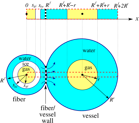
Fig. 3: (Bottom) A 2D cross-section through a fiber–vessel pair showing the water, ice and gas regions, and the moving interfaces. (Top) The 1D region corresponding to our simplified model geometry is outlined with a red, dashed box in the bottom figure. The locations of the various phase boundaries are indicated, with the origin $x=0$ at the center of the fiber.

Model equations are derived for the fiber and vessel compartments in the next two sections. For easy reference, all parameters and variables are listed in Table 1 along with physical values where appropriate. There are some similarities that can be found with other models developed for related problems such as ice lensing in porous soils [24] and freeze/thaw processes in the food industry [11]; however, neither problem contains all of the physical mechanisms encountered during sap exudation.

Table 1: A list of nomenclature for all physical parameters and variables, including values in SI units. References are given for each numerical value, either as a citation to the literature (in square brackets) or else an equation number (in parentheses) for those values calculated from other parameters.

	Description	Units	Value	Ref.
Constant parameters:
$A$	Area of vessel wall that is permeable	$\mathrm{m^{2}}$	$6.28\times 10^{-8}$	(18)
$c_{s}$	Sucrose concentration in vessel sap	$\mathrm{mol/m^{3}}$	58.4
$g$	Gravitational acceleration	$\mathrm{m/s^{2}}$	9.81	[30]
$h$	Heat transfer coefficient	$\mathrm{W/m^{2}\,{}^{\circ}K}$	10.0	[17]
$H$	Henry’s constant	–	0.0274	[19]
$k_{g}$	Thermal conductivity of air	$\mathrm{W/m\,{}^{\circ}K}$	0.0243	[1]
$k_{w}$	Thermal conductivity of water	$\mathrm{W/m\,{}^{\circ}K}$	0.580	[1]
$K$	Cell wall hydraulic conductivity	$\mathrm{m/s}$	$1.98\times 10^{-14}$	[16]
$0pt^{f}$	Length of fiber	$\mathrm{m}$	$1.0\times 10^{-3}$	[15]
$0pt^{v}$	Length of vessel element	$\mathrm{m}$	$0.5\times 10^{-3}$	[15]
$M_{g}$	Molar mass of air	$\mathrm{kg/mol}$	0.0290	[30]
$M_{s}$	Molar mass of sucrose	$\mathrm{kg/mol}$	0.3423	[30]
$N$	Number of fibers per vessel	–	16	(16)
$\hat{p}$	Pressure scale	$\mathrm{N/m^{2}}$	$1.01\times 10^{5}$	(32)
$R^{f}$	Interior radius of fiber	$\mathrm{m}$	$3.5\times 10^{-6}$	[33]
$R^{v}$	Interior radius of vessel	$\mathrm{m}$	$2.0\times 10^{-5}$	[33]
${\cal R}$	Universal gas constant	$\mathrm{J/mol\,{}^{\circ}K}$	8.314	[30]
$\hat{t}$	Time scale	$\mathrm{s}$	46.1	(43)
$T_{c}$	Freezing temperature of ice	$\mathrm{{}^{\circ}K}$	273.15
$T_{a}$	Ambient temperature of gas	$\mathrm{{}^{\circ}K}$	$0.005+T_{c}$
$V^{f}$	Volume of fiber	$\mathrm{m^{3}}$	$3.85\times 10^{-14}$	(4)
$V^{v}$	Volume of vessel	$\mathrm{m^{3}}$	$6.28\times 10^{-13}$	(31)
$W$	Thickness of fiber + vessel wall	$\mathrm{m}$	$3.64\times 10^{-6}$	[31]
$\lambda$	Latent heat of fusion	$\mathrm{J/kg}$	$3.34\times 10^{5}$	[1]
$\rho_{i}$	Ice density	$\mathrm{kg/m^{3}}$	917	[1]
$\rho_{w}$	Water density	$\mathrm{kg/m^{3}}$	1000	[30]
$\hat{\rho}$	Density scale	$\mathrm{kg/m^{3}}$	1.29	[26]
$\sigma$	Air-water surface tension	$\mathrm{N/m}$	0.0756	[30]
Dependent and independent variables:
$c_{g}$	Dissolved gas concentration	$\mathrm{mol/m^{3}}$
$m$	Mass	$\mathrm{m}$
$p$	Pressure	$\mathrm{N/m^{2}}$
$r$	Radius of gas bubble in vessel	$\mathrm{m}$
$s$	Fiber interface location	$\mathrm{m}$
$t$	Time	$\mathrm{s}$
$T$	Temperature	$\mathrm{{}^{\circ}K}$
$U$	Volume of melted ice	$\mathrm{m^{3}}$
$V$	Volume	$\mathrm{m^{3}}$
$x$	Spatial location	$\mathrm{m}$
$\rho$	Density	$\mathrm{kg/m^{3}}$
Subscript (denotes phase):
$g$	Gas phase
$i$	Ice phase
$w$	Water phase
Superscript (denotes cell component):
$f$	Fiber
$v$	Vessel

3.1 Fiber model

We now develop a set of governing equations for the fiber that is restricted to the time period when ice is present, so that an ice layer separates the gas from the water adjacent to the wall. The modifications that are required to the model once the ice layer has disappeared and the fiber bubble is in direct contact with the sap are described in Section 3.5.

The inner fiber wall is initially coated by an ice layer of uniform thickness, inside of which is a cylindrical volume of compressed gas with radius $s_{gi}(t)$. As the ice layer melts, an ice/water interface $x=s_{iw}(t)$ appears at the inner edge of the fiber wall ($s_{iw}(0)=R^{f}$) and propagates inward. The speed of the interface depends not only on the volume difference between ice and water but also on the seepage of liquid through the porous fiber wall. The gas pressure that drives water through the wall into the vessel is transmitted through the ice layer to the adjacent water.

If we denote by $V^{f}_{g}(t)$, $V^{f}_{w}(t)$ and $V^{f}_{i}(t)$ the volumes of gas, water and ice within the fiber, then owing to the cylindrical symmetry

$$V^{f}_{g}(t) =\pi 0pt^{f}\,s_{gi}(t)^{2},$$ (1)

$$V^{f}_{w}(t) =\pi 0pt^{f}\left((R^{f})^{2}-s_{iw}(t)^{2}\right),$$ (2)

$$V^{f}_{i}(t) =\pi 0pt^{f}\left(s_{iw}(t)^{2}-s_{gi}(t)^{2}\right),$$ (3)

which also satisfy

$$V^{f}_{g}(t)+V^{f}_{w}(t)+V^{f}_{i}(t)=\pi 0pt^{f}\left(R^{f}\right)^{2}=:V^{f}.$$ (4)

Recalling Assumption A10, which takes the gas temperature $T^{f}_{g}$ to be constant and equal to the freezing point $T_{c}=273.15\,\mbox{$\mathrm{{}^{\circ}K}$}$, the gas density varies only due to changes in volume so that

$$\rho^{f}_{g}(t)=\rho^{f}_{g}(0)\,\frac{V^{f}_{g}(0)}{V^{f}_{g}(t)}.$$ (5)

The corresponding gas pressure is given by the ideal gas law

$$p^{f}_{g}(t)=\frac{\rho^{f}_{g}(t){\cal R}T_{c}}{M_{g}},$$

where $M_{g}$ is the molar mass of air. This can be combined with (1) and (5) to obtain

$$p^{f}_{g}(t)=p^{f}_{g}(0)\,\left(\frac{s_{gi}(0)}{s_{gi}(t)}\right)^{2}.$$ (6)

As ice thaws, some volume of melt-water (denoted $U(t)$) is forced through the fiber wall into the vessel, while the remainder stays in the fiber sandwiched between the ice layer and the wall. Let the (constant) mass of gas in the fiber be $m^{f}_{g0}$ and the mass of water and ice be

$$m^{f}_{i}(t)=\rho_{i}V^{f}_{i}(t),$$ (7)

$$m^{f}_{w}(t)=\rho_{w}V^{f}_{w}(t),$$ (8)

where $\rho_{w}$ and $\rho_{i}$ are the densities of water and ice respectively. Conservation of mass in the fiber implies that

$$m^{f}_{g0}+m^{f}_{i}(t)+m^{f}_{w}(t)+\rho_{w}U(t)=m^{f}_{0},$$ (9)

where initially $U(0)=0$ and $m^{f}_{0}=m^{f}_{g0}+m^{f}_{i}(0)+m^{f}_{w}(0)$. Differentiating (9) yields

$$\dot{m}^{f}_{i}(t)+\dot{m}^{f}_{w}(t)+\rho_{w}\dot{U}(t)=0,$$

where the “dot” denotes a time derivative. Substituting (4) and (7)–(8) into the last expression yields

$$-\rho_{i}\dot{V}^{f}_{g}+(\rho_{w}-\rho_{i})\dot{V}^{f}_{w}+\rho_{w}\dot{U}=0,$$

and the volume terms can be replaced using (1) and (2) to obtain

$$2\rho_{i}s_{gi}\dot{s}_{gi}+2(\rho_{w}-\rho_{i})s_{iw}\dot{s}_{iw}-\frac{\rho_{w}}{\pi 0pt^{f}}\,\dot{U}=0.$$ (10)

Recall that the temperature in both gas and ice is assumed constant and equal to the freezing point $T_{c}$. The water layer, on the other hand, is heated from the vessel side so that the water temperature $T^{f}_{w}(x,t)$ is not constant but instead obeys the steady-state heat equation and boundary condition

$$\partial_{xx}T^{f}_{w} =0\qquad\text{for all}\;x\in\left(s_{iw},R^{f}\right),$$ (11a)

$$T^{f}_{w} =T_{c}\qquad\text{at}\;x=s_{iw}.$$ (11b)

The speed $\dot{s}_{iw}$ of the ice/water interface is determined by the Stefan condition

$$\lambda\rho_{w}\dot{s}_{iw}=-k_{w}\partial_{x}T^{f}_{w}\qquad\text{at}\;x=s_{iw},$$ (12)

where $\lambda$ is the latent heat of fusion and $k_{w}$ is the thermal conductivity of water.

In summary, (6), (10), (11a) and (12) represent a coupled system of equations for the fiber unknowns $s_{iw}(t)$, $s_{gi}(t)$, $p^{f}_{g}(t)$, and $T^{f}_{w}(x,t)$. In the next section, we will derive an equation for $\dot{U}$ and also determine the missing boundary condition for $T^{f}_{w}$ as a matching condition with the vessel temperature at the fiber/vessel wall $x=R^{f}$.

3.2 Vessel model and matching conditions

Let $V^{v}_{w}(t)$ and $V^{v}_{g}(t)$ denote the volume of the water and gas compartments. The time derivative of the total volume (gas + water) must be zero so that

$$\frac{d}{dt}\left(V^{v}_{w}(0)+NU(t)+V^{v}_{g}(t)\right)=0,$$

or simply

$$\dot{V}^{v}_{g}=-N\dot{U}.$$ (13)

This equation embodies the assumption that there is no flow between vessel elements so that the portion of the volume consisting of water equals the initial value $V^{v}_{w}(0)$ plus whatever water enters from the $N$ surrounding fibers. Using the fact that the bubble radius and volume are connected by

$$V^{v}_{g}(t)=\pi 0pt^{v}\,r(t)^{2},$$ (14)

equation (13) can then be rewritten as

$$r\dot{r}=-\frac{N\dot{U}}{2\pi 0pt^{v}}.$$ (15)

Assuming that fibers are packed tightly around the vessel and that both vessel and fiber have wall thickness $W$, a simple geometric argument provides an estimate for the constant $N$:

$$N\approx\frac{2\pi(R^{f}+R^{v}+W)}{2R^{f}+W}.$$ (16)

We next focus on porous transport through the fiber wall which is governed by Darcy’s law

$$N\dot{U}(t)=-\frac{KA}{\rho_{w}gW}(p^{v}_{w}(t)-p^{f}_{g}(t)),$$ (17)

where $p^{v}_{w}(t)$ is the vessel water pressure, $K$ is the hydraulic conductivity, $W$ is the wall thickness, and $A$ is the area of the wall that is permeable to water. In the absence of experimental measurements for hydraulic conductivity in maple, we use the value $K=1.98\times 10^{-14}\;\mbox{$\mathrm{m/s}$}$ obtained for birch trees [16]. Finally, $A$ is taken equal to the internal surface area of the cylindrical vessel

$$A=2\pi R^{v}0pt^{v}.$$ (18)

We next describe the temperature evolution within the various vessel compartments, recalling that the diffusive time scale is short in relation to either melting or gas dissolution. We therefore employ a quasi-steady approximation in which temperatures obey a steady-state heat equation. Denote by $T^{v}_{g}(x,t)$ the temperature within the gas bubble, and $T_{w1}^{v}(x,t)$ and $T_{w2}^{v}(x,t)$ the water temperatures to the left and right of the bubble respectively. Then, in the water region on the left (adjacent to the vessel wall) $T_{w1}^{v}(x,t)$ obeys

$$\partial_{xx}T_{w1}^{v} =0\qquad \text{for all}\;x \in\left(R^{f},R^{f}+R^{v}-r\right).$$ (19a)

Both temperature and heat flux are continuous at the vessel wall

$$T_{w1}^{v} =T^{f}_{w}\qquad \text{at}\;x =R^{f},$$ (19b)

$$k_{w}\partial_{x}T_{w1}^{v} =k_{w}\partial_{x}T^{f}_{w}\qquad \text{at}\;x =R^{f},$$ (19c)

and at the water/gas interface

$$T_{w1}^{v} =T^{v}_{g}\qquad \text{at}\;x =R^{f}+R^{v}-r,$$ (19d)

$$k_{w}\partial_{x}T_{w1}^{v} =k_{g}\partial_{x}T^{v}_{g}\qquad \text{at}\;x =R^{f}+R^{v}-r.$$ (19e)

The gas temperature $T^{v}_{g}(x,t)$ inside the bubble obeys

$$\partial_{xx}T^{v}_{g} =0\qquad \text{for all}\;x \in\left(R^{f}+R^{v}-r,R^{f}+R^{v}+r\right),$$ (20a)

with temperature and flux continuity conditions

$$T^{v}_{g} =T_{w2}^{v}\qquad \text{at}\;x =R^{f}+R^{v}+r,$$ (20b)

$$k_{g}\partial_{x}T^{v}_{g} =k_{w}\partial_{x}T_{w2}^{v}\qquad \text{at}\;x =R^{f}+R^{v}+r.$$ (20c)

Finally, the water temperature $T_{w2}^{v}(x,t)$ to the right of the gas obeys

$$\partial_{xx}T_{w2}^{v} =0\qquad \text{for all}\;x \in\left(R^{f}+R^{v}+r,R^{f}+2R^{v}\right),$$ (21a)

with a Robin condition on the right-most boundary

$$k_{w}\partial_{x}T_{w2}^{v} =h(T_{a}-T_{w2}^{v})\qquad \text{at}\;x =R^{f}+2R^{v},$$ (21b)

where $h$ is a convective heat transfer coefficient. The ambient temperature $T_{a}$ refers to the temperature in the neighboring layer of xylem cells; using a temperature difference of $10\mbox{$\mathrm{{}^{\circ}K}$}$ through the sapwood over a tap depth of 0.05 $\mathrm{m}$, we obtain a rough estimate of $T_{a}\approx 0.005\mbox{$\mathrm{{}^{\circ}K}$}$ for the temperature difference on the cell scale.

The final component of the model is a description of the process whereby elevated pressures in the gas bubble cause the gas to dissolve at the gas/water interface. Because of the small bubble size, it is essential to take into account the effect of surface tension. Gas and liquid pressures in the vessel are connected by the Young–Laplace equation,

$$p^{v}_{w}(t)=p^{v}_{g}(x,t)-\frac{\sigma}{r(t)}\qquad\text{at $x=R^{f}+R^{v}-r$},$$ (22)

where $\sigma$ is the air-water surface tension and $r(t)$ is the bubble radius. In this formula, the gas pressure can be written using the ideal gas law

$$p^{v}_{g}(x,t)=\frac{\rho^{v}_{g}(t){\cal R}T^{v}_{g}(x,t)}{M_{g}},$$ (23)

where $\rho^{v}_{g}(t)$ is the gas density which we have taken uniform in space according to Assumption A11. The concentration $c^{v}_{g}(t)$ of dissolved gas in the sap is then related to the gas density by Henry’s law

$$c^{v}_{g}(t)=\frac{H}{M_{g}}\rho^{v}_{g}(t),$$ (24)

where $H$ is a dimensionless constant. The gas density in the preceding equations decreases over time owing to dissolution and can be written

$$\rho^{v}_{g}(t)=\frac{\rho^{v}_{g}(0)V^{v}_{g}(0)-M_{g}\int_{\Omega^{v}_{w}}c^{v}_{g}(t)\,dV}{V^{v}_{g}(t)}=\frac{\rho^{v}_{g}(0)V^{v}_{g}(0)-M_{g}c^{v}_{g}(t)(V^{v}-V^{v}_{g}(t))}{V^{v}_{g}(t)},$$ (25)

where $V^{v}_{g}(t)$ is given by (14) and the integral in the first expression is taken over $\Omega_{w}$, the annular portion of the vessel filled with liquid.

In summary, equations (15), (17) and (19)–(25) represent a nonlinear system of differential-algebraic equations for the nine unknown functions $r(t)$, $p^{v}_{w}(t)$, $p^{v}_{g}(x,t)$, $T_{w1}^{v}(x,t)$, $T_{w2}^{v}(x,t)$, $T^{v}_{g}(x,t)$, $\rho^{v}_{g}(t)$, $c^{v}_{g}(t)$ and $U(t)$. The vessel and fiber solutions are coupled via matching conditions (17), (19b) and (19c).

3.3 Osmotic effects

Tyree and co-workers have argued that a pressurized gas bubble in the xylem will dissolve entirely over a period of 12 hours or less, so that some other pressure-generating mechanism must operate to sustain the bubbles actually observed in xylem sap [5, 26, 28]. Recent experiments by Cirelli et al. [5] suggest that the fiber secondary wall is selectively-permeable, allowing water to pass through but preventing the passage of larger molecules such as sucrose and thereby generating a significant osmotic potential difference between fibers and vessels. This leads naturally to the hypothesis that osmotic pressure might provide the extra mechanism needed to enhance flow of sap from fiber to vessel and hence prevent bubbles in the fiber from totally dissolving once the ice layer has completely melted.

Osmosis can be described mathematically by means of the Morse equation that relates osmotic pressure $\Pi$ within a solution to the dissolved solute concentration $c_{s}$ via $\Pi=c_{s}{\cal R}T$.  Following the approach in [18], we apply this equation to the sap solutions in fiber and vessel and hence obtain a modified version of the melt volume equation (17)

$$N\dot{U}=-\frac{KA}{\rho_{w}gW}\,\left[(p^{v}_{w}-p^{f}_{g})-{\cal R}T^{f}_{w}(R^{f},t)\,(c^{v}_{s}-c^{f}_{s})\right],$$

where $c^{f}_{s}$ and $c^{v}_{s}$ are the sucrose concentrations in the fiber and vessel respectively. According to Tyree and Zimmermann [28], sucrose is present only in the vessels, so that $c^{f}_{s}\equiv 0$ and

$$N\dot{U}=-\frac{KA}{\rho_{w}gW}\,\left[(p^{v}_{w}-p^{f}_{g})-{\cal R}T^{f}_{w}(R^{f},t)c^{v}_{s}\right].$$ (26)

This equation replaces (17), but otherwise the governing equations remain unchanged. For the sake of simplicity, we assume that the vessel sucrose concentration $c^{v}_{s}$ is a constant which for a 2% sucrose solution corresponds to taking $c^{v}_{s}=0.02\rho_{w}/M_{s}\approx 58.4\;\mbox{$\mathrm{mol/m^{3}}$}$, where the molar mass of sucrose is $M_{s}=0.3423\;\mbox{$\mathrm{kg/mol}$}$. This assumption can be justified by arguing that ray parenchyma cells (which provide the bulk of the sucrose to the tree vascular system) are so numerous in maples that they should be capable of maintaining the sucrose concentration at a relatively constant level.

3.4 Non-dimensional variables

To simplify the governing equations, we reduce the number of parameters in the problem by introducing the following change of variables:

$$\begin{array}[]{ccc}x=R^{v}\bar{x},&s=R^{v}\bar{s},&r=R^{v}\bar{r},\\[5.69046pt] t=\hat{t}\,\bar{t},&U=V^{v}\bar{U},&p=\hat{p}\,\bar{p},\\[5.69046pt] \rho=\hat{\rho}\,\bar{\rho},&c=\frac{\hat{\rho}}{M_{g}}\,\bar{c},&T=T_{c}+(T_{a}-T_{c})\bar{T},\end{array}$$ (30)

where an overbar denotes a dimensionless quantity. The melt volume is non-dimensionalized using

$$V^{v}=\pi 0pt^{v}(R^{v})^{2},$$ (31)

density and pressure scales are chosen based on initial values as

$$\hat{\rho}=\rho^{v}_{g}(0)\qquad\text{and}\qquad\hat{p}=p^{v}_{g}(0)=\frac{\hat{\rho}{\cal R}T_{c}}{M_{g}},$$ (32)

and the time scale $\hat{t}$ will be specified shortly.

The above expressions are then substituted into the dimensional equations from Section 3, after which we immediately simplify notation by dropping asterisks. The differential equations and boundary conditions (11) and (19)–(21) governing the temperatures $\bar{T}^{f}_{w}(x,t)$, $\bar{T}^{v}_{w1}(x,t)$, $\bar{T}^{v}_{w2}(x,t)$ and $\bar{T}^{v}_{g}(x,t)$ become:

Fiber water: $$\partial_{\bar{x}\bar{x}}\bar{T}_{w}^{f} =0\qquad\qquad\quad\;\;\; \text{for all}\;\bar{x} \in\left(s_{iw},\delta\right),$$ (33a)

$$\bar{T}_{w}^{f} =0\qquad \text{at}\;\bar{x} =s_{iw},$$ (33b)

Vessel water (left): $$\partial_{\bar{x}\bar{x}}\bar{T}^{v}_{w1} =0\qquad\qquad\quad\;\;\; \text{for all}\;\bar{x} \in\left(\delta,\delta+1-\bar{r}\right),$$ (34a)

$$\bar{T}^{v}_{w1} =\bar{T}^{f}_{w}\qquad \text{at}\;\bar{x} =\delta,$$ (34b)

$$\partial_{\bar{x}}\bar{T}^{v}_{w1} =\partial_{\bar{x}}\bar{T}^{f}_{w}\qquad\quad \text{at}\;\bar{x} =\delta,$$ (34c)

$$\bar{T}^{v}_{w1} =\bar{T}^{v}_{g}\qquad \text{at}\;\bar{x} =\delta+1-\bar{r},$$ (34d)

$$\partial_{\bar{x}}\bar{T}^{v}_{w1} =\eta\partial_{\bar{x}}\bar{T}^{v}_{g}\qquad \text{at}\;\bar{x} =\delta+1-\bar{r},$$ (34e)

Vessel gas bubble: $$\partial_{\bar{x}\bar{x}}\bar{T}^{v}_{g} =0\qquad\qquad\quad\;\; \text{for all}\;\bar{x} \in\left(\delta+1-\bar{r},\delta+1+\bar{r}\right),$$ (35a)

$$\bar{T}^{v}_{g} =\bar{T}^{v}_{w2}\qquad \text{at}\;\bar{x} =\delta+1+\bar{r},$$ (35b)

$$\eta\partial_{\bar{x}}\bar{T}^{v}_{g} =\partial_{\bar{x}}\bar{T}^{v}_{w2}\qquad \text{at}\;\bar{x} =\delta+1+\bar{r},$$ (35c)

Vessel water (right): $$\partial_{\bar{x}\bar{x}}\bar{T}^{v}_{w2} =0 \text{for all}\;\bar{x} \in\left(\delta+1+\bar{r},\delta+2\right),\qquad\;\;$$ (36a)

$$\partial_{\bar{x}}\bar{T}^{v}_{w2} =\mathrm{Bi}(1-\bar{T}^{v}_{w2})\quad \text{at}\;\bar{x} =\delta+2.$$ (36b)

The dimensionless parameter $\mathrm{Bi}=hR^{v}/k_{w}$ is the Biot number.

Next are five algebraic equations for $\bar{p}^{f}_{g}(\bar{t})$, $\bar{p}^{v}_{g}(\bar{x},\bar{t})$, $\bar{p}^{v}_{w}(\bar{t})$, $\bar{c}^{v}_{g}(\bar{t})$ and $\bar{\rho}^{v}_{g}(\bar{t})$:

$$\bar{p}^{f}_{g}=\bar{p}^{f}_{g}(0)\,\left(\frac{\bar{s}_{gi}(0)}{\bar{s}_{gi}}\right)^{2},$$ (37)

$$\bar{p}^{v}_{g}=\bar{\rho}^{v}_{g}(1+\theta\bar{T}^{v}_{g}),$$ (38)

$$\bar{p}^{v}_{w}=\bar{p}^{v}_{g}-\frac{\omega}{\bar{r}},$$ (39)

$$\bar{c}^{v}_{g}=H\bar{\rho}^{v}_{g},$$ (40)

$$\bar{\rho}^{v}_{g}=\frac{(\bar{r}(0))^{2}-\bar{c}^{v}_{g}(1-\bar{r}^{2})}{\bar{r}^{2}}.$$ (41)

The non-dimensionalized Stefan condition (12) becomes

$$\dot{\bar{s}}_{iw}=-\partial_{\bar{x}}\bar{T}^{f}_{w}\qquad\text{at}\;\bar{x}=\bar{s}_{iw},$$ (42)

where we have chosen the time scale

$$\hat{t}=\frac{\lambda\rho_{w}(R^{v})^{2}}{k_{w}(T_{a}-T_{c})},$$ (43)

so as to eliminate the coefficient in the Stefan condition. This is clearly an appropriate time scale for our problem because the melting process governs the dynamics of the ice layer and hence also the water transport from fiber to vessel. Using parameter values from Table 1, we find that a typical value of the time scale is $\hat{t}\approx 46.1\;\mbox{$\mathrm{s}$}$. Finally, the remaining differential equations (10), (15) and (17) for the quantities $\bar{s}_{gi}(\bar{t})$, $\bar{r}(\bar{t})$ and $\bar{U}(\bar{t})$ become

$$2\beta\bar{s}_{gi}\dot{\bar{s}}_{gi}+2(1-\beta)\bar{s}_{iw}\dot{\bar{s}}_{iw}-\gamma\dot{\bar{U}}=0,$$ (44)

$$2\bar{r}\dot{\bar{r}}=-N\dot{\bar{U}},$$ (45)

$$N\dot{\bar{U}}=-\alpha\left[\bar{p}^{v}_{w}-\bar{p}^{f}_{g}-(1+\theta\bar{T}^{f}_{w}(\delta,\bar{t}))\bar{c}^{v}_{s}\right].$$ (46)

Table 2: A list of dimensionless parameters and their numerical values.

Symbol	Definition	Value
$\mathrm{Bi}$	$\frac{hR^{v}}{k_{w}}$	$3.45\times 10^{-4}$
$\alpha$	$\frac{KA\hat{p}\hat{t}}{\rho_{w}gWV^{v}}$	0.258
$\beta$	$\frac{\rho_{i}}{\rho_{w}}$	0.917
$\gamma$	$\frac{0pt^{v}}{0pt^{f}}$	0.500
$\delta$	$\frac{R^{f}}{R^{v}}$	0.175
$\eta$	$\frac{k_{g}}{k_{w}}$	0.0419
$\theta$	$\frac{T_{a}-T_{c}}{T_{c}}$	$1.83\times 10^{-5}$
$\omega$	$\frac{\sigma}{\hat{p}R^{v}}$	0.0374

3.5 Onset of gas dissolution in fiber after ice melts completely

As the ice in the fiber melts, we eventually reach a critical time when the ice layer disappears and the two interfaces $\bar{s}_{gi}$ and $\bar{s}_{iw}$ merge into a single gas–water interface whose position we denote by $\bar{x}=\bar{s}(\bar{t})$. Similar to the gas/water interface in the vessel, the dynamics of $\bar{s}$ are governed by dissolution of gas within the fiber water and changes in pressure/volume of the gas bubble. Assuming as before that the gas in the fiber diffuses much faster than it dissolves, we again employ a quasi-steady approximation in which the dissolved gas concentration is assumed constant at any given time. Therefore, we replace (37) with

$$\bar{p}^{f}_{g}=\bar{\rho}^{f}_{g}(1+\theta\bar{T}^{f}_{g})=\bar{\rho}^{f}_{g},$$ (47)

and eliminate (42) and (44) in favor of the single equation

$$2\bar{s}\dot{\bar{s}}=\gamma\dot{\bar{U}}.$$ (48)

These last two equations are already dimensionless and are analogous to (38) and (45) for the vessel. The modified system has as additional unknowns the water pressure $\bar{p}^{f}_{w}$, dissolved gas concentration $\bar{c}^{f}_{g}$, and gas density $\bar{\rho}^{f}_{g}$, which are governed by the following analogues of the vessel equations (41) and (40):

$$\bar{p}^{f}_{w}=\bar{p}^{f}_{g}-\frac{\omega}{\bar{s}}$$ (49)

$$\bar{c}^{f}_{g}=H\bar{\rho}^{f}_{g},$$ (50)

$$\bar{\rho}^{f}_{g}=\frac{\xi(\bar{s}_{gi}(0))^{2}-\bar{c}^{f}_{g}(1-\bar{s}^{2})}{\bar{s}^{2}},$$ (51)

where $\xi=\rho^{f}_{g}(0)/\rho^{v}_{g}(0)$ is a dimensionless parameter corresponding to the ratio of initial gas densities. Finally, without the ice layer to transmit the gas pressure directly to the fiber water located on the other side, Darcy’s law (46) must be modified so as to replace the fiber gas pressure by $\bar{p}^{f}_{w}$:

$$N\dot{\bar{U}}=-\alpha\left[\bar{p}^{v}_{w}-\bar{p}^{f}_{w}-(1+\theta\bar{T}^{f}_{w}(\delta,\bar{t}))\bar{c}^{v}_{s}\right].$$ (52)

3.6 Analytical solution for temperatures

Because the quasi-steady temperature equations (33)–(36) have such a simple form, they can be solved analytically. In fact, the temperature is a linear function of $\bar{x}$ in each sub-domain, and applying the corresponding boundary and matching conditions leads to the following explicit solutions in terms of $\bar{x}$, $\bar{t}$ and the non-dimensional parameters:

$$\bar{T}^{f}_{w}(\bar{x},\bar{t})\equiv\bar{T}^{v}_{w1}(\bar{x},\bar{t}) =\frac{\eta(\bar{x}-\bar{s}_{iw}(\bar{t}))}{\eta(\delta+2+\mathrm{Bi}^{-1})+2(1-\eta)\bar{r}(\bar{t})-\eta\bar{s}_{iw}(\bar{t})},$$ (53)

$$\bar{T}^{v}_{g}(\bar{x},\bar{t}) =\frac{\bar{x}-(1-\eta)\left(\delta+1-\bar{r}(\bar{t})\right)-\eta\bar{s}_{iw}(\bar{t})}{\eta(\delta+2+\mathrm{Bi}^{-1})+2(1-\eta)\bar{r}(\bar{t})-\eta\bar{s}_{iw}(\bar{t})},$$ (54)

$$\bar{T}^{v}_{w2}(\bar{x},\bar{t}) =\frac{\eta\bar{x}+2(1-\eta)\bar{r}(\bar{t})-\eta\bar{s}_{iw}(\bar{t})}{\eta(\delta+2+\mathrm{Bi}^{-1})+2(1-\eta)\bar{r}(\bar{t})-\eta\bar{s}_{iw}(\bar{t})}.$$ (55)

The temperature solution on the whole domain may then be summarized as

$$\bar{T}(\bar{x},\bar{t})=\begin{cases}0,&\text{if $\bar{x}\in[0,\,\bar{s}_{iw}]$,}\\ \bar{T}^{f}_{w}(\bar{x},\bar{t}),&\text{if $\bar{x}\in(\bar{s}_{iw},\,\delta+1-\bar{r}]$,}\\ \bar{T}^{v}_{g}(\bar{x},\bar{t}),&\text{if $\bar{x}\in(\delta+1-\bar{r},\,\delta+1+\bar{r}]$,}\\ \bar{T}^{v}_{w2}(\bar{x},\bar{t}),&\text{if $\bar{x}\in(\delta+1+\bar{r},\,\delta+2]$.}\end{cases}$$ (56)

Note that the matching conditions on temperature and heat flux at the vessel wall imply that the functions $\bar{T}^{f}_{w}$ and $\bar{T}^{v}_{w1}$ are identical.

3.7 Initial conditions

We choose a “base case” for our simulations in which the initial conditions are taken consistent with the typical scenario described by Tyree [26]:

• $p^{v}_{g}(0)=100\;\mbox{$\mathrm{kPa}$}$: gas in the vessel is initially at atmospheric pressure.

• $p^{f}_{g}(0)=200\;\mbox{$\mathrm{kPa}$}$: gas in the fiber is at twice the pressure in the vessel owing to compression by the frozen sap. Based on Tyree’s data, we expect that this value is an upper bound, so that $p^{f}_{g}(0)$ actually lies in the range $[100,200]\;\mbox{$\mathrm{kPa}$}$.

• $\bar{s}_{iw}(0)=\delta$, $\bar{s}_{gi}(0)=\delta/\sqrt{2}\approx 0.7\delta$ and $\bar{U}(0)=0$: corresponding to a fiber gas bubble that is initially half the total fiber volume, with the other half filled by ice. This initial state is established during the previous fall/winter freeze, when gas-filled fibers are at atmospheric pressure in equilibrium with the vessels. As the temperature falls below freezing, ice forms on the inside of the fiber wall and the gas pressure increases by a factor inversely proportional to the ice thickness according to equation (37); hence, the value $\bar{s}_{gi}(0)=0.7\delta$ is consistent with the initial gas pressures chosen above.

• $\bar{r}(0)$: is the quantity in this study with the greatest uncertainty since we haven’t yet found data on gas concentration or bubble size in the vessels; hence, this is a natural parameter to vary in our simulations. We expect that the initial vessel volume fraction taken up by gas is significantly less than in the fiber, otherwise a large embolus is likely to remain in the vessel and hinder sap transport once transpiration recommences.

Initial values are not required for the temperatures, although they can be obtained by substituting the above values into (53)–(56) and the algebraic relations in Section 3.4.

4 Numerical simulations

Owing to the nonlinear coupling in the governing equations derived in the previous section, numerical simulations are required in order to obtain solutions of the full system. We employ a straightforward numerical approach in which the four ordinary differential equations (42) and (44)–(46) are solved for $\bar{s}_{gi}$, $\bar{s}_{iw}$, $\bar{r}$ and $\bar{U}$ using the stiff solver ode15s in MATLAB, with error tolerances $\text{RelTol}=10^{-10}$ and $\text{AbsTol}=10^{-8}$. Temperatures are calculated using the analytical expressions in (53)–(55), and the system is closed using the algebraic equations (37)–(41).

The above procedure applies when ice is present in the fiber. In order to permit MATLAB to modify the equations automatically once the ice disappears, the event detection feature in ode15s is used to determine the instant when $\bar{s}_{gi}=\bar{s}_{iw}$ and $V^{f}_{i}\rightarrow 0$; at this time, the simulation is halted and the calculation is restarted with the equations modified as described in Section 3.5. To assist in understanding which equations are solved under which circumstances, we have provided in Figure 4 a graphical summary of the equations and variables in the two cases.

[rowsep=0.8,colsep=0.5]

Fig. 4: List of variables and governing equations depending on whether or not ice is present in the fiber.

In the remainder of this section, we perform a series of simulations with increasing model complexity, first studying the dynamics of gas dissolution and flow through the fiber wall when the pressurized fibers contain no ice, then introducing osmotic effects, and finally incorporating the ice layer and phase change. Even though the code is written in dimensionless variables, all parameters and results from this point on are converted to dimensional variables using equations (30).

4.1 Case 1: Dissolution and porous transport only (no ice, no osmosis)

We begin by considering the simple situation in which there is no sucrose in the vessel and no ice in the fiber (and hence, no phase change). As a result, the sap dynamics are governed primarily by two effects: gas dissolution and the flow of sap driven by pressure exchange between gas bubbles in the fiber and vessel. We note that temperature variations are relatively small and so they have a negligible effect on the solution.

Gas bubble dissolution has been studied extensively in the context of sap flow by several authors [10, 21, 33], who concluded based on experimental evidence and simple physical arguments that pressurized gas bubbles in xylem sap should dissolve completely over a time period ranging anywhere from 20 minutes to several hours. These results are partially supported by the mathematical study of bubble dissolution by Keller [9], who proved that for an under-saturated solution (such as xylem sap) that fills an unbounded domain, the only stable equilibrium solution is one in which the gas bubble shrinks and eventually disappears. An analogous situation was studied by Yang and Tyree [33], who performed experiments on excised maple branches open to the air and developed a corresponding mathematical model in which the pressure is maintained at atmospheric conditions at the open boundary. Their experimental and numerical results are consistent with the complete dissolution of gas bubbles in finite time.

In our study of sap exudation however, we are interested in the behavior of xylem sap within an intact maple tree stem that is not exposed to the open air; consequently, the open boundary conditions treated by Yang-Tyree above are not applicable here. Fortunately, Keller also considered a pressurized gas bubble suspended in a closed fluid container [9] for which he proved that the bubble will still shrink in size as it dissolves, but in this case will reach an equilibrium state having non-zero radius. This behavior is contrary to that observed above in experiments on excised maple branches, and so bears careful consideration.

To investigate the ability of our model to capture Keller’s results for a closed container, we performed several simulations with bubbles of various sizes in both fiber and vessel. We start with a scenario in which the fiber bubble takes up 50% of the fiber volume and the vessel bubble only 10%, corresponding to $s_{gi}(0)=R^{f}/\sqrt{2}\approx 0.7R^{f}$ and $r(0)=R^{v}/\sqrt{10}\approx 0.3R^{v}$. Based on the discussion of initial conditions in Section 3.7, the gas in the vessel is initially at atmospheric pressure (100 $\mathrm{kPa}$) while that in the fiber is twice as large (200 $\mathrm{kPa}$). The resulting dynamics for the pressures and bubble radii are shown in Figure 5, from which we observe that the fiber bubble grows in size while the vessel bubble shrinks, until both reach an equilibrium state at a time of roughly $t=40$ seconds. Figure 5(a) shows shows that the system approaches an equilibrium state in which the water pressure in the two compartments is equal (at approximately 155 $\mathrm{kPa}$). This is clearly consistent with (46) since there can be no flux across the porous cell wall at the equilibrium state, which requires that $\bar{p}^{f}_{w}=\bar{p}^{g}_{w}$ (remembering also that $\bar{c}^{v}_{s}=0$). The plots show that the gas and water pressures vary inversely with the radii as expected, and the piecewise linear dependence of temperature on position in equations (53)–(56) is evident in Figure 5(d).

(a) Water pressures	(b) Gas pressures	(c) Gas bubble radii
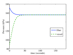
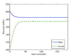
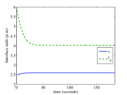
	(d) Temperatures

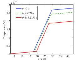
Fig. 5: Case 1 – base case: No ice, initial radii $s(0)=0.7R^{f}$, $r(0)=0.3R^{v}$, and pressure $p^{f}_{g}(0)=200\;\mbox{$\mathrm{kPa}$}$.

The plot of gas pressure shows a decrease in $p^{f}_{g}$ over time as the fiber bubble expands and a corresponding decrease in $p^{v}_{g}$ as the vessel bubble is compressed. This behavior is consistent with Keller’s results for bubbles in a closed system, and also captures the transfer of pressure from fiber to vessel that we would expect in sap exudation. It is important to note that the increase in vessel water pressure from roughly 90 to 155 $\mathrm{kPa}$ (see Figure 5(a)) is close to the upper limit of the range of 30–60 $\mathrm{kPa}$ that is to be expected for positive pressures in maple according to [25]. Finally, we note that the magnitude of the pressure change in the fiber arising from dissolution of gas is only 5 $\mathrm{kPa}$, which is small relative to the other pressure differences between fiber and vessel; consequently, dissolution has only a small effect on sap flow over this time scale.

The parameter value with the most uncertainty is the initial value of vessel bubble radius, and so we focus next on the effect of reducing $r(0)$ in Figure 6. As long as $r(0)$ is greater than approximately $0.2R^{v}$, we observe behavior similar to the earlier simulations in Figure 5 in that the fiber gas bubble expands, driving water through the cell wall and hence compressing the gas in the vessel. However, when $r(0)=0.2R^{v}$ the vessel gas bubble dissolves entirely, causing the gas pressure to become unbounded as $r\rightarrow 0$ owing to the air/water surface tension term in (39). At the precise moment when the vessel bubble disappears, the model breaks down because there is no further transfer of pressure between fiber and vessel, nor is there any flow of sap through the fiber/vessel wall. This point actually corresponds to a terminal steady state of the system, and in our computations we have found it necessary to specify a very small threshold value of the bubble radius below which we halt the simulation. The collapsing vessel bubble case $r(0)=0.2R^{v}$ is illustrated in more detail in the plots in Figure 7.

The dissolution of gas in the vessel has an intriguing connection with the phenomenon of embolism repair [33], in which gas bubbles within the vessel that could potentially hinder sap transport are known to dissolve during the spring thaw. The physical mechanism underlying embolism repair is still not fully understood, and has implications for a wide range of other tree species; hence, a more detailed study of bubble dissolution as relates to embolism would form a fascinating avenue for future research.

(a) Vessel bubble radius		(b) Vessel water pressure

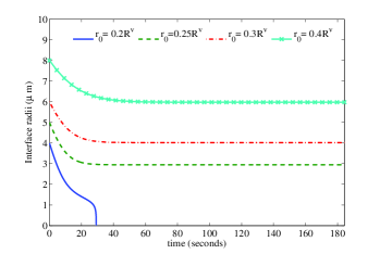
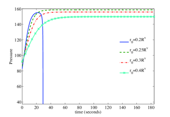
Fig. 6: Case 1 – varying $r(0)$: No ice, initial radius $s(0)=0.7R^{f}$, and pressure $p^{f}_{g}(0)=200\;\mbox{$\mathrm{kPa}$}$.

(a) Water pressures	(b) Gas pressures	(c) Gas bubble radii

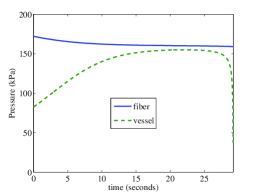
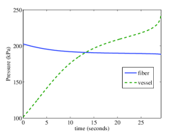
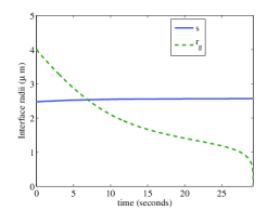
Fig. 7: Case 1 – collapsing vessel bubble: No ice, initial radii $s(0)=0.7R^{f}$, $r(0)=0.2R^{v}$, and pressure $p^{f}_{g}(0)=200\;\mbox{$\mathrm{kPa}$}$. Here, the initial vessel bubble is so small that it dissolves entirely.

Since $p^{f}_{g}(0)=200\;\mbox{$\mathrm{kPa}$}$ is at the upper end of the range of fiber gas pressures we would expect in actual trees, we next consider the effect of varying $p^{f}_{g}(0)$ over the range $[100,200]\;\mbox{$\mathrm{kPa}$}$. As seen in Figure 8, the qualitative behavior is similar until the initial fiber gas pressure approaches the atmospheric level in the vessel; for $p^{f}_{g}(0)$ low enough, the dynamics are reversed in the sense that the fiber bubble shrinks and the vessel bubble expands. As seen in the detailed plots for $p^{f}_{g}(0)=100\;\mbox{$\mathrm{kPa}$}$ in Figure 9, the fiber and vessel again equilibrate at a state where the water pressures are equal, although in this case the level of $p_{w}\approx 75\;\mbox{$\mathrm{kPa}$}$ is much lower than that observed in the base case. Clearly, when the fiber begin at lower pressure, then the tree is less able to pressurize the vessel sap; furthermore, the fiber compartment must be above some threshold pressure for there to be any pressure transfer from fiber to vessel that is consistent with exudation.

(a) Vessel bubble radius		(b) Vessel water pressure

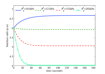
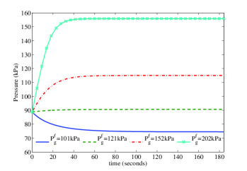
Fig. 8: Case 1 – varying $p^{f}_{g}(0)$: No ice, initial radii $s(0)=0.7R^{f}$, $r(0)=0.3R^{v}$.

(a) Water pressures	(b) Gas pressures	(c) Gas bubble radii

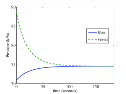
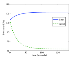
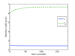
Fig. 9: Case 1 – reduced fiber pressure: No ice, initial radii $s(0)=0.7R^{f}$ and $r(0)=0.3R^{v}$, and pressure $p^{f}_{g}(0)=100\;\mbox{$\mathrm{kPa}$}$.

In fact, if the initial fiber gas pressure and radius are both small enough, then it is the gas in the fiber that dissolves entirely. Although this situation is not likely to occur in practice, we have nonetheless included a simulation with $p^{f}_{g}(0)=100\;\mbox{$\mathrm{kPa}$}$ and $s(0)=0.25R^{f}$ in Figure 7 to illustrate this point.

(a) Water pressures	(b) Gas pressures	(c) Gas bubble radii

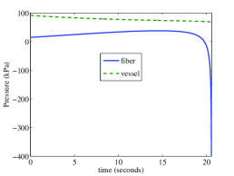
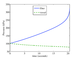
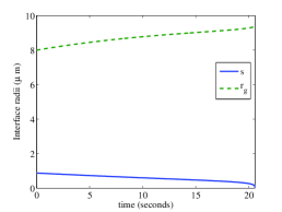
Fig. 10: Case 1 – collapsing fiber bubble: No ice, initial radii $s(0)=0.25R^{f}$, $r(0)=0.4R^{v}$, and pressure $p^{f}_{g}(0)=100\;\mbox{$\mathrm{kPa}$}$. The fiber bubble radius and pressure are initially so small in this case that the fiber bubble dissolves entirely.

4.2 Case 2: No ice, with osmosis

For the next round of simulations, we introduce osmotic effects arising from the presence of sucrose in the vessel, and still maintain our focus on the effect of porous flow and gas dissolution by assuming all sap is in the liquid phase. The vessel sap is taken to contain 2% sucrose by mass (with 0% in the fiber), but otherwise the initial conditions are similar to Case 1.

The first simulation with $r(0)=0.3R^{v}$, $p^{v}_{g}(0)=100\;\mbox{$\mathrm{kPa}$}$ and $p^{f}_{g}(0)=200\;\mbox{$\mathrm{kPa}$}$ is displayed in Figure 11 and should be compared with Figure 5 (base case, without osmosis). Osmotic pressure has a relatively small impact on the fiber bubble dynamics, with the fiber radius being only slightly smaller and the equilibrium water pressure dropping from 155 $\mathrm{kPa}$ to just under 150 $\mathrm{kPa}$. In contrast, there is a major change in the vessel bubble evolution, with the equilibrium radius dropping to roughly half that of the base case. The source of the difference is evident from the pressure plots: the initial vessel water pressure is nearly 140 $\mathrm{kPa}$ lower than the base case in Figure 5(a) owing to the osmotic pressure, and the equilibrium vessel gas pressure increases by roughly the same amount.

Maintaining the fiber bubble at pressure $p^{f}_{g}(0)=100\;\mbox{$\mathrm{kPa}$}$, we next draw comparisons with Figure 6 which varied the vessel bubble radius over values $r(0)=\{0.2,0.25,0.3,0.4\}R^{v}$. From the summary of results shown in Figure 12, we see that the presence of osmosis enhances the flow from fiber to vessel and leads to a much larger pressure increase in the vessel sap. The smallest vessel gas bubble with $r(0)=0.2$ disappears sooner in the presence of osmosis, which is to be expected.

A more insightful comparison is afforded by reducing the fiber gas pressure to $p^{f}_{g}(0)=100\;\mbox{$\mathrm{kPa}$}$, and comparing Figure 13 to the corresponding case without osmosis in Figure 9 (where we observed a reversed sap flow, from vessel to fiber). Clearly, osmotic effects act to return the sap dynamics to “normal,” with water now being driven from fiber to vessel. Except for the shift in equilibrium pressures, the qualitative solution behavior is now consistent with the base case simulation in Figure 5. Consequently, our model demonstrates that osmotic pressures owing to sucrose in the vessel can provide a mechanism for enhancing sap exudation, even when the gas pressure in the fiber is as low as that in the vessel. In this respect, our model is consistent with the hypothesis of Tyree [26] that claims osmosis prevents gas bubble dissolution in the fiber and sustains sap exudation pressures over longer time periods.

(a) Water pressures	(b) Gas pressures	(c) Gas bubble radii

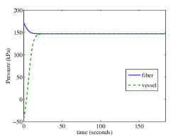
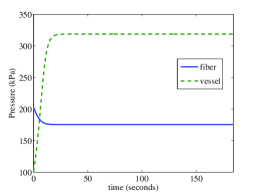
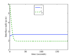
Fig. 11: Case 2 – base case with osmosis: No ice, with osmosis, initial radii $s(0)=0.7R^{f}$, $r(0)=0.3R^{v}$, and pressure $p^{f}_{g}(0)=200\;\mbox{$\mathrm{kPa}$}$.

(a) Vessel bubble radius		(b) Vessel water pressure

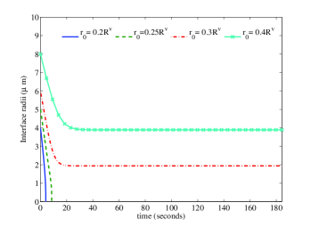
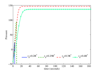
Fig. 12: Case 2 – varying $r(0)$: No ice, with osmosis, initial radius $s(0)=0.7R^{f}$, and pressure $p^{f}_{g}(0)=200\;\mbox{$\mathrm{kPa}$}$.

(a) Water pressures	(b) Gas pressures	(c) Gas bubble radii

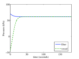
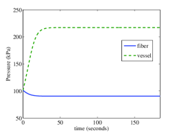
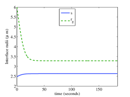
Fig. 13: Case 2 – reduced fiber pressure: No ice, with osmosis, initial radii $s(0)=0.7R^{f}$, $r(0)=0.3R^{v}$, and pressure $p^{f}_{g}(0)=100\;\mbox{$\mathrm{kPa}$}$.

4.3 Case 3: Milburn–O’Malley model (with ice, no osmosis)

We next test Milburn and O’Malley’s hypothesis for sap exudation that includes the effects of melting ice and gas dissolution, but ignores osmosis. We restrict ourselves to the time period over which ice is present, so that gas in the fiber is isolated from the water phase by the frozen ice layer and hence gas dissolution occurs only in the vessel (the long-time dynamics after the ice layer melts are considered in Case 5). Furthermore, gas–water interfacial tension plays no role in the fiber in this case, so that the pressure of the melted liquid adjacent to the fiber wall is simply equal to the gas pressure.

In Figure 14, we present the simulation results using initial conditions $s_{gi}=0.7R^{f}$, $s_{wi}=R^{f}$, $r(0)=0.3R^{v}$, $p^{f}_{g}(0)=200~{}\mbox{$\mathrm{kPa}$}$ and $p^{v}_{g}(0)=100~{}\mbox{$\mathrm{kPa}$}$, which can be compared with the base case depicted in Figure 5. Until a time of roughly 40 $\mathrm{s}$, the qualitative features of the two solutions are similar, with the water pressure decreasing in the fiber and increasing in the vessel until they equilibrate at some intermediate value. Over this time period, the fiber bubble radius increases smoothly from the initial $2.45\;\mbox{$\mathrm{\mu m}$}$ to roughly $2.6\;\mbox{$\mathrm{\mu m}$}$, and the motion of the vessel bubble (not shown) is also similar to that of the base case. There is, however, a significant difference in the gas and water pressures owing to the absence of surface tension.

After the initial rapid equilibration phase, the two water pressures remain equal and experience a gradual decrease over a much longer time scale. This slow adjustment in pressure is due to phase change and is attributed to the roughly 10% difference in density between water and ice. The ice/water interface $s_{iw}(t)$ has a roughly linear variation in time according to Figure 14(c), which should be contrasted with the $\sqrt{t}$ dependence that typically arises in Stefan problems; this discrepancy is due to the fact that sap outflow through the fiber wall dominates the interface motion. The intersection of the $s_{gi}$ and $s_{iw}$ curves near $t\approx 2000\;\mbox{$\mathrm{s}$}$ represents the time when the ice layer disappears. Our main conclusion from these results is that even when ice is present, the vessel compartment is pressurized by the fiber, with the main difference (comparing Figures 5 and 14) being that the vessel sap pressure is higher because of the missing interfacial tension force.

A final series of simulations is then performed in which the initial vessel bubble radius is varied over the range $r(0)=\{0.2,0.25,0.3,0.4\}R^{v}$. Figure 15 shows that the smallest bubble dissolves entirely within approximately 10 seconds, after which the transfer of pressure from fiber to vessel stops. In all other cases, the fiber and vessel compartments equilibrate over a time scale of roughly 2 hours.

(a) Water pressures	(b) Gas pressures	(c) Fiber phase interfaces

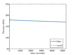
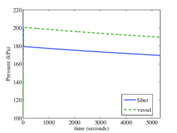
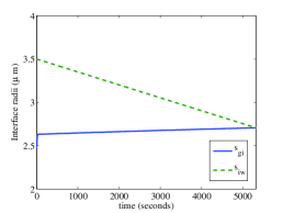
Fig. 14: Case 3 – base case with ice: Milburn–O’Malley scenario, no osmosis. Initial radii are $s_{gi}(0)=0.7R^{f}$, $s_{iw}=R^{f}$, $r(0)=0.3R^{v}$, and pressure $p^{f}_{g}(0)=200\;\mbox{$\mathrm{kPa}$}$.

(a) Vessel bubble radius		(b) Vessel water pressure

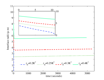
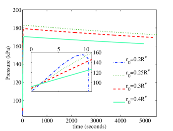
Fig. 15: Case 3 – varying $r(0)$: Milburn–O’Malley scenario with ice and no osmosis, initial radius $s(0)=0.7R^{f}$, and pressure $p^{f}_{g}(0)=200\;\mbox{$\mathrm{kPa}$}$. The “zoomed-in” sub-plot shows the curves near $t=0$.

4.4 Case 4: Full model, with ice and osmosis

In this section, we simulate the full model including ice and osmosis, beginning again with the base case. The solution plots displayed in Figure 16 should be compared with the Milburn–O’Malley simulation in Figure 14, which differs only in the lack of osmosis. The two sets of results are qualitatively similar, there being slight changes in the water pressure and bubble radii owing to the inclusion of osmotic pressure. Consistent with the ice-free results in Cases 1 and 2, the vessel gas pressure is increased by an amount roughly equal to the osmotic pressure $\Pi=c_{s}{\cal R}T\approx 132\;\mbox{$\mathrm{kPa}$}$.

If the initial vessel bubble radius is decreased slightly from $0.30R^{v}$ to $0.29R^{v}$, then the vessel bubble is no longer unable to equilibrate with the fiber and dissolves completely as shown in Figure 17. This is consistent with the other results in Figures 7 and 12, except that the extra osmotic pressure in the vessel causes the gas to disappear at larger values of $r(0)$. When viewed in the context of embolism recovery, this is evidence that suggests osmosis can enhance the ability of the tree to recover from embolism.

A series of simulations for different values of the initial vessel bubble radius are reported in Figure 18, which shows a similar outcome as in Case 3. The main difference is that the bubbles with radii $r(0)=0.2R^{v}$ and $0.25R^{v}$ both dissolve completely, which is further evidence that osmosis enhances the effect of exudation and makes the vessel bubbles more likely to collapse.

(a) Water pressures	(b) Gas pressures	(c) Fiber phase interfaces

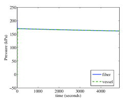
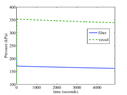
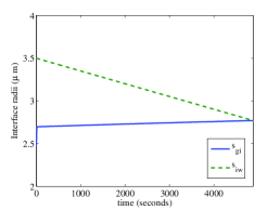
Fig. 16: Case 4 – base case with ice and osmosis: Initial radii $s_{gi}(0)=0.7R^{f}$, $r(0)=0.3R^{v}$, and pressure $p^{f}_{g}(0)=200\;\mbox{$\mathrm{kPa}$}$.

(a) Water pressures	(b) Gas pressures	(c) Gas bubble radii

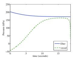
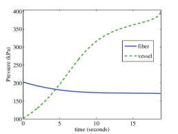
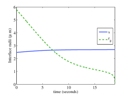
Fig. 17: Case 4 – collapsing vessel bubble: With ice and osmosis, initial radii $s_{gi}(0)=0.7R^{f}$, $r(0)=0.29R^{v}$, and pressure $p^{f}_{g}(0)=200\;\mbox{$\mathrm{kPa}$}$.

(a) Vessel bubble radius		(b) Vessel gas pressure

Fig. 18: Case 4 – varying $r(0)$: With ice and osmosis, initial fiber radius $s_{gi}(0)=0.7R^{f}$, and pressure $p^{f}_{g}(0)=200\;\mbox{$\mathrm{kPa}$}$. The endpoint of each curve corresponds to the time that the ice layer completely melts. The “zoomed-in” sub-plot shows the curves near $t=0$.

4.5 Case 5: Long-time behavior after ice melts completely

The purpose of this final set of simulations is to study the behavior over the longer term once the ice is totally melted, and to demonstrate that our approach is capable of computing through the disappearance of the ice layer and the corresponding change in the governing equations. We present results for a few choices of parameters considered in the previous section (Case 4) and emphasize that until the time that the ice melts, the plots are identical. Our main observation is that after the ice disappears, the solution dynamics exhibit a rapid equilibration to a constant equilibrium state that is consistent with what we saw earlier in Case 2 (no ice, with osmosis).

Simulations are shown in Figures 19 and 20 for two values of vessel radius, $r(0)=0.3$ and $0.6$, that can be compared with results in Figure 16 and 18. At the instant the ice layer melts away, the water pressures undergo a sudden transition in which $p^{f}_{w}$ and $p^{v}_{w}$ drop sharply and then rapidly equilibrate to a new constant value. This pressure discontinuity arises from the sudden appearance of the surface tension term in equation (49), when the ice layer vanishes and the fiber sap comes into contact with the gas. We emphasize here that the numerical algorithm handles the discontinuity and change in governing equations easily and without introducing any spurious oscillations or other non-physical effects.

After the jump in water pressure, there is a rapid but smooth variation in the radii and gas pressure as the system equilibrates (although in the case when $r(0)=0.3R^{v}$ the change in gas pressure is too small to be seen on this scale). Otherwise, the behavior after the loss of ice is analogous to the earlier ice-free simulations.

In reality, we would expect to see a rapid but smooth variation in liquid surface tension as the disappearing ice layer transitions through a “mushy region” where both ice and water coexist [lacey-tayler-1983]. Including this additional level of detail would not have a major effect on our solution, but it could form the basis for an interesting future study of the detailed structure of the transition layer.

(a) Water pressures	(b) Gas pressures	(c) Gas bubble radii

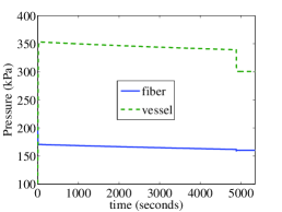
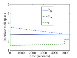
Fig. 19: Case 5 – base case with ice and osmosis: Long-time behavior with initial radii $s_{gi}(0)=0.7R^{f}$, $r(0)=0.3R^{v}$, and pressure $p^{f}_{g}(0)=200\;\mbox{$\mathrm{kPa}$}$.

(a) Water pressures	(b) Gas pressures	(c) Gas bubble radii

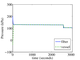
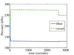
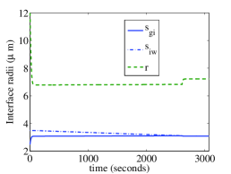
Fig. 20: Case 5 – larger vessel bubble: With ice and osmosis, initial radii $s_{gi}(0)=0.7R^{f}$, $r(0)=0.6R^{v}$, and pressure $p^{f}_{g}(0)=200\;\mbox{$\mathrm{kPa}$}$.

5 Conclusions and future work

The aim of this work was to develop a detailed mathematical model that captures the physical effects – heat and mass transport, gas dissolution, surface tension, osmosis and phase change – that are believed to play a significant role in sap exudation in maple trees. In particular, we were interested in investigating two competing hypotheses for sap exudation based on a model of Milburn–O’Malley (without osmosis) [12] and another of Tyree (with osmosis) [26]. The model focuses on the cellular scale and the transfer of pressure between two main xylem components: fibers and vessels. We derived a coupled system of nonlinear, time-dependent, differential-algebraic equations, which we solved using MATLAB. Extensive numerical simulations were performed that uncovered the following:

• It is necessary to include the effect of gas bubbles in the vessel sap in order to allow a transfer of stored pressure in the fibers to the vessel sap. This gas in the vessels was not explicitly mentioned by either Milburn–O’Malley or Tyree.

• Taking parameter values consistent with data in the literature, our model captures positive vessel pressures provided that the gas in the fiber is sufficiently compressed during the previous year’s freezing phase. The observed increase in vessel sap pressure lies in the range of 30–60 $\mathrm{kPa}$ that is consistent with experimental values reported in the literature for maple sap exudation.

• For a wide range of parameters, and provided the vessel gas content is low enough, the fibers are able to completely dissolve the gas bubbles within the vessel sap. This is consistent with the phenomenon of embolism repair that is known to occur in maple as well as other hardwood species.

• Reasonable exudation pressures are obtained both with and without osmosis. One impact of including osmotic effects is to increase slightly the threshold vessel bubble size below which gas in the vessel gas dissolves entirely; in this respect, our model suggests that osmosis may enhance embolism repair. The second main impact of osmosis is to lessen the likelihood that the fiber gas bubble collapses, which enhances the ability to exude sap.

This paper can only be considered as a preliminary study of sap exudation because the comparisons and conclusions we have drawn so far are mainly qualitative. More detailed comparisons with experimental data in the literature are currently underway to further validate the model, and will form the basis of a future publication. There are a number of other specific areas that we believe would provide fruitful avenues for future research:

• The long-time behavior pictured in Figures 19 and 20 suggests that this problem is ripe for a multi-layer asymptotic analysis in which the solution is divided into two pieces: a linear solution, matched to initial conditions via a boundary layer on the left; and a constant equilibrium state that is matched across an interior layer to the linear solution.

• The predictive power of this model would be strengthened with better estimates of two parameters: the gas content in the vessel, and the initial pressure in the fiber. We will perform a more extensive search of the literature and focus in particular on data from studies of embolism. In conjunction with this effort, we believe that our model (with only minor modifications) could also be applied to study the phenomenon of embolism repair coinciding with the spring thaw [33].

• The conditions under which the maple tree freezes at the end of the previous season are known to have a significant impact on sap exudation during the following spring. To study this process, we could run our model “in reverse” to study the cooling sequence in the Milburn–O’Malley model (steps 1–4 in Figure 2).

• We are currently developing a macroscopic tree-level model, based on the 1D model of Chuang et al. [3] that uses Richards’ equation to capture sap flow in the porous xylem. In order to apply this work to the study of exudation, we require solution-dependent transport coefficients that will be derived from the microscopic cell-level model derived in the current paper using an up-scaling procedure.

References

- [1] The Engineering ToolBox. http://www.engineeringtoolbox.com/, accessed on Apr. 28, 2012.
- [2] T. Améglio, F. W. Ewers, H. Cochard, M. Martignac, M. Vandame, C. Bodet, and P. Cruiziat. Winter stem xylem pressure in walnut trees: effects of carbohydrates, cooling and freezing. Tree Physiol., 21:387–394, 2001.
- [3] Y.-L. Chuang, R. Oren, A. L. Bertozzi, N. Phillips, and G. G. Katul. The porous media model for the hydraulic system of a conifer tree: Linking sap flux data to transpiration rate. Ecol. Model., 191:447–468, 2006.
- [4] D. Cirelli. Anatomy and physiology of sugar maple (Acer saccharum Marsh.) in relation to xylem sap pressure. Master’s thesis, University of Maine, Aug. 2005.
- [5] D. Cirelli, R. Jagels, and M. T. Tyree. Toward an improved model of maple sap exudation: the location and role of osmotic barriers in sugar maple, butternut and white birch. Tree Physiol., 28:1145–1155, 2008.
- [6] P. M. Cortes and T. R. Sinclair. The role of osmotic potential in spring sap flow of mature sugar maple trees (Acer saccharum marsh.). J. Exp. Bot., 36(1):12–24, 1985.
- [7] L. P. V. Johnson. Physiological studies on sap flow in the sugar maple, Acer saccharum marsh. Can. J. Res. C: Bot. Sci., 23:192–197, 1945.
- [8] R. W. Johnson, M. T. Tyree, and M. A. Dixon. A requirement for sucrose in xylem sap flow from dormant maple trees. Plant Physiol., 84:495–500, 1987.
- [9] J. B. Keller. Growth and decay of gas bubbles in liquids. In R. Davies, editor, Cavitation in Real Liquids: Proceedings of the Symposium on Cavitation in Real Liquids, pages 19–29. General Motors Research Laboratories, Warren, Michigan, Elsevier, 1964.
- [10] W. Konrad and A. Roth-Nebelsick. The dynamics of gas bubbles in conduits of vascular plants and implications for embolism repair. J. Theor. Biol., 224:43–61, 2003.
- [11] R. W. Lewis and K. N. Seetharamu. Heat and mass transfer in food processing. IMA J. Math. Appl. Bus. Ind., 5:303–324, 1995.
- [12] J. A. Milburn and P. E. R. O’Malley. Freeze-induced sap absorption in Acer pseudoplatanus: a possible mechanism. Can. J. Bot., 62(10):2101–2106, 1984.
- [13] J. A. Milburn and M. H. Zimmermann. Sapflow in the sugar maple in the leafless state. J Plant Physiol., 124:331–344, 1986.
- [14] S. G. Pallardy. Physiology of Woody Plants. Elsevier, Amsterdam, third edition, 2007.
- [15] A. J. Panshin and C. de Zeeuw. Textbook of Wood Technology. McGraw-Hill, New York, fourth edition, 1980.
- [16] J. A. Petty and M. A. Palin. Permeability to water of the fibre cell wall material of two hardwoods. J. Exp. Bot., 34(143):688–693, 1983.
- [17] B. E. Potter and J. A. Andresen. A finite-difference model of temperatures and heat flow within a tree stem. Can. J. For. Res., 32:548–555, 2002.
- [18] A. Radu, J. Vrouwenvelder, M. van Loosdrecht, and C. Picioreanu. Modeling the effect of biofilm formation on reverse osmosis performance: Flux, feed channel pressure drop and solute passage. J. Membrane Sci., 365(1-2):1–15, 2010.
- [19] R. Sander. Compilation of Henry’s law constants for inorganic and organic species of potential importance in environmental chemistry. Max Planck Institute of Chemistry, Mainz, Germany, Downloaded from http://www.rolf-sander.net/henry, April 8, 1999.
- [20] J. J. Sauter, W. Iten, and M. H. Zimmermann. Studies on the release of sugar into the vessels of sugar maple (Acer saccharum). Can. J. Bot., 51(1):1–8, 1973.
- [21] F. Shen, L. Wenji, G. Rongfu, and H. Hu. A careful physical analysis of gas bubble dynamics in xylem. J. Theor. Biol., 225:229–233, 2003.
- [22] J. S. Sperry, J. R. Donnelly, and M. T. Tyree. Seasonal occurrence of xylem embolism in sugar maple (Acer saccharum). Amer. J. Bot., 75(8):1212–1218, 1988.
- [23] C. L. Stevens and R. L. Eggert. Observations on the causes of the flow of sap in red maple. Plant Physiol., 20:636–648, 1945.
- [24] F. Talamucci. Freezing processes in porous media: Formation of ice lenses, swelling of the soil. Math. Comput. Modelling, 37:595–602, 2003.
- [25] M. T. Tyree. Maple sap uptake, exudation, and pressure changes correlated with freezing exotherms and thawing endotherms. Plant Physiol., 73:277–285, 1983.
- [26] M. T. Tyree. The mechanism of maple sap exudation. In M. Terazawa, C. A. McLeod, and Y. Tamai, editors, Tree Sap: Proceedings of the 1st International Symposium on Sap Utilization, pages 37–45, Bifuka, Japan, April 10–12, 1995. Hokkaido University Press.
- [27] M. T. Tyree and F. W. Ewers. The hydraulic architecture of trees and other wood plants. New Phytol., 119:345–360, 1991.
- [28] M. T. Tyree and M. H. Zimmermann. Xylem Structure and the Ascent of Sap. Springer Series in Wood Science. Springer-Verlag, Berlin, second edition, 2002.
- [29] Universe Review. Anatomy of plants. Web site: http://universe-review.ca/R10-34-anatomy2.htm.
- [30] W. R. Veazey et al., editors. CRC Handbook of Chemistry and Physics. CRC Press, 75th edition, 1994.
- [31] P. Watson, A. Hussein, S. Reath, W. Gee, J. Hatton, and J. Drummond. The kraft pulping properties of Canadian red and sugar maple. Tappi J., 2(6):26–32, 2003.
- [32] K. M. Wiegand. Pressure and flow of sap in wood. Amer. Nat., 40(474):409–453, 1906.
- [33] S. Yang and M. T. Tyree. A theoretical model of hydraulic conductivity recovery from embolism with comparison to experimental data on Acer saccharum. Plant Cell Env., 15:633–643, 1992.