Amplification and suppression of system-bath correlation effects in an open many-body system

Abstract

Understanding the rich dynamics of open quantum systems is of fundamental interest to quantum control and quantum information processing. By considering an open system of many identical two-level atoms interacting with a common bath, we show that effects of system-bath correlations are amplified in a many-body system via the generation of a short time scale inversely proportional to the number of atoms. Effects of system-bath correlations are therefore considerable even when each individual atom interacts with the bath weakly. We further show that correlation-induced dynamical effects may still be suppressed via the dynamical decoupling approach, but they present a challenge for quantum state protection as the number of atom increases.

I Introduction

The rich dynamics of open quantum systems continues to attract great interests breuerbook . Two main motivations for now are to achieve better quantum control and to better understand possible quantum effects in large systems. However, the general complexity of open quantum systems puts exact solutions out of reach. A variety of approximations or assumptions are therefore needed, with their validity under close scrutiny in recent years due to fascinating experimental advances in, e.g., cold-atom physics and photonics. One common assumption in treating open quantum systems, often referred to as “factorized initial conditions”, is that the system and the environment are initially uncorrelated. This can be justified for weak system-bath coupling because the system has a negligible impact on the bath statistics PollakPRE2008 . On the other hand, for moderate and strong system-bath coupling, which is the case in some realistic situations of great experimental interest (e.g., light-harvesting systems, super-conducting qubits, and atom-cavity systems), initial system-bath correlations (SBCs) should be accounted for PechukasPRL ; RoyerPRL ; Hanggi ; TanimuraPRL2010 ; cheekong .

Pioneering studies of SBCs in single-body systems, e.g., a single spin or a single harmonic oscillator in a thermal bath, have been fruitful HakimPRA1985 ; HaakePRA1985 ; Grabert1988 ; SmithPRA1990 ; GrabertPRE1997 ; PazPRA1997 ; LutzPRA2003 ; BanerjeePRE2003 ; vanKampen2004 ; BanPRA2009 ; UchiyamaPRA ; SmirnePRA2010 ; DajkaPRA ; TanPRA2011 ; MorozovPRA2012 ; wgwang (Refs. TanimuraPRL2010 ; ZhangPRA2010 are notable exceptions involving two spins). The main purpose of this work is to extend the investigation to a system of many identical two-level atoms, where novel collective phenomena might occur (one example is super-radiance Dicke1954 ). Specifically, we consider a system of many identical two-level atoms, each atom weakly interacting with a common bath. Using an exactly solvable model, we show below that effects of SBCs may dramatically increase with the number of atoms $N$, leading to a previously unknown time scale $t_{c}$ inversely proportional to $N$. For a large system with many atoms, $t_{c}$ becomes very small and SBCs manifest themselves by inducing rapid oscillations in physical observables. Three implications of our findings are in order. First, the collective dynamics of many two-level atoms can be strongly affected by SBCs even when each individual two-level atom interacts weakly with the bath. Second, this fact may be exploited to amplify and gauge SBCs. Third, a small $t_{c}$ presents challenges for quantum state protection via dynamical decoupling (DD) techniques. In general, it is found that SBCs force us to apply more frequent and more efficient DD pulses to freeze the quantum evolution.

In Sec. II, we present our theoretical findings of SBC effects in a model system consisting of $N$ two-level atoms in a common bath. Section III presents computational examples. We then discuss in Sec. IV the implications for the dynamical decoupling technique and how it may be used to suppress SBC effects. Section V gives a brief summary. Readers interested in the technical details of our derivations should refer to Appendices A-D.

II System-bath correlation effects in a system of $N$ two-level atoms in a common bath

A collection of $N$ identical two-level atoms interacting with a common bosonic bath may be described by an extended spin-boson Hamiltonian $H_{\text{total}}=H_{S}+H_{B}+H_{\text{int}}$ (setting $\hbar=1$ throughout) VorrathChemPhys2004 ; VorrathPRL2005 , with

$$H_{S} = \omega_{0}J_{z}+\delta J_{x}+\chi J_{z}^{2};$$ (1)

$$H_{B} = \sum_{k}\omega_{k}b_{k}^{\dagger}b_{k},$$ (2)

$$H_{\text{int}} = 2J_{z}\sum_{k}(g_{k}^{*}b_{k}+g_{k}b_{k}^{\dagger}).$$ (3)

Here $J_{x,y,z}$ are the collective spin operators with $J_{x}^{2}+J_{y}^{2}+J_{z}^{2}=\frac{N}{2}(\frac{N}{2}+1)$, $\omega_{0}$ is the energy bias, $\chi$ the interaction between the atoms, $\delta$ is the tunneling amplitude, and $H_{B}$ is a collection of boson modes or harmonic oscillators (with zero-point energy dropped). Such a total Hamiltonian $H_{\text{total}}$ can model a two-mode BEC interacting via collisions with thermal atoms or phonon excitations KurizkiPRL2011 . We stress that, other than the self-interaction term $\chi J_{z}^{2}$, $H_{\text{total}}$ is nothing but a straightforward extension of the standard spin-boson model Weissbook to a model of many spins interacting with a common bath.

Rather than switching on the system-bath interaction $H_{\text{int}}$ at a particular instant, in most physical situations the system and the bath have interacted for a long time beforehand. Our starting point is then a thermal equilibrium state for the system and the bath as a whole at temperature $T$, i.e., $\rho\propto\exp(-\beta H_{\text{total}})$ with $\beta\equiv\frac{1}{k_{b}T}$. Noticing the energy contribution by $H_{\text{int}}$, one finds that the associated reduced state of the system (bath) is not really given by $\rho_{S}^{\text{eq}}\varpropto e^{-\beta H_{S}}$ ($\rho_{B}^{\text{eq}}\varpropto e^{-\beta H_{B}}$) Weissbook ; cheekong . Instead, states of the system and of the bath are correlated for a non-vanishing $H_{\text{int}}$. Now, if at time $t=0$, the system is prepared in a pure state $\left|\psi\right\rangle$ via a projective measurement, then the initial state of the system and the bath as a whole is given by

$$\rho(0)=\left|\psi\right\rangle\left\langle\psi\right|\otimes\frac{\left\langle\psi\right|e^{-\beta H_{\text{total}}}\left|\psi\right\rangle}{Z},$$ (4)

where $Z$ is a normalization factor. This initial state should be compared with the usual uncorrelated (unphysical) initial state,

$$\rho^{\text{dir}}(0)=\left|\psi\right\rangle\left\langle\psi\right|\otimes\frac{e^{-\beta H_{B}}}{\text{Tr}_{B}(e^{-\beta H_{B}})}.$$ (5)

Evidently, for a nonzero $H_{\text{int}}$, we have $\rho(0)\neq\rho^{\text{dir}}(0)$. That is, the physical initial state in Eq. (4) has correctly accounted for the system-bath interaction during the past. Consequently the initial bath state $\rho_{B}(0)=\left\langle\psi\right|e^{-\beta H_{\text{total}}}\left|\psi\right\rangle/Z$ depends on $H_{\text{int}}$ as well as the state preparation of the system and is therefore not a canonical equilibrium state for the bath. Previously, how the difference between $\rho(0)$ and $\rho^{\text{dir}}(0)$ impacts on the ensuing dynamics was studied for a damped harmonic oscillator (see, e.g., Ref. PazPRA1997 ) and a single two-level system undergoing pure dephasing MorozovPRA2012 . In Appendices C and D, we also consider initial states of the form $\Omega e^{-\beta H_{\text{total}}}\Omega^{\dagger}/Z$, where $\Omega$ is a unitary operator acting on the system Hilbert space, and we argue that this initial state for large $N$ leads to similar results as $\rho(0)$ does.

In general, the dynamics of $H_{\text{total}}$ starting from $\rho(0)$ or $\rho^{\text{dir}}(0)$ does not have analytical solutions. To obtain analytical solutions from which important insights may be gained, we set the tunneling parameter $\delta$ in $H_{S}$ to zero, yielding a pure-dephasing problem for collective spin states. In the context of a two-mode BEC, such a situation arises if intermode coherent tunneling is made to vanish and if intermode mixing collisions are negligible. Purely for convenience, we shall assume $\chi=0$, which may be achieved via Feshbach resonance. Up to a unitary transformation, one can obtain equivalent situations if $\omega_{0}=0$ and if inter-mode mixing collisions dominate KurizkiPRL2011 .

Working in the basis of $J_{z}$ eigenstates, denoted by $|m\rangle$ with $J_{z}\left|m\right\rangle=m\left|m\right\rangle$, we first find the system’s reduced density matrix for the uncorrelated initial state $\rho^{\text{dir}}(0)$ (see Appendices for detailed calculations),

$$[\rho_{S}(t)]_{mn} =[\rho_{S}(0)]_{mn}e^{-i\omega_{0}(m-n)t}e^{-i\Delta(t)(m^{2}-n^{2})t}$$

$$\times e^{-\gamma(t)(m-n)^{2}t},$$ (6)

where the decoherence factor is given by

$$\gamma(t)=\sum_{k}4|g_{k}|^{2}\frac{(1-\cos(\omega_{k}t))}{\omega_{k}^{2}t}\coth\left(\frac{\beta\omega_{k}}{2}\right),$$ (7)

and

$$\Delta(t)=\sum_{k}4|g_{k}|^{2}\left(\frac{\sin(\omega_{k}t)-\omega_{k}t}{\omega_{k}^{2}t}\right).$$ (8)

The factor $\exp[-i\Delta(t)(m^{2}-n^{2})t]$ arises because the common bosonic bath assists in generating an indirect atom-atom interaction. Note that at sufficiently short times for which $\sin(\omega_{k}t)\approx\omega_{k}t$, we have $\Delta(t)\approx 0$.

By contrast, for the physical initial state $\rho(0)$ in Eq. (4), we find

$$[\rho_{S}(t)]_{mn} =[\rho_{S}(0)]_{mn}e^{-i\omega_{0}(m-n)t}e^{-i\Delta(t)(m^{2}-n^{2})t}$$

$$\times e^{-\gamma(t)(m-n)^{2}t}F^{c}_{mn}(t)$$ (9)

where

$$F^{c}_{mn}(t)=\sum_{l}p_{l}e^{-i\left[2l(n-m)\sum_{k}4|g_{k}|^{2}\sin(\omega_{k}t)/\omega_{k}^{2}\right]},$$ (10)

with the probability

$$p_{l}=\dfrac{|\langle l|\psi\rangle|^{2}e^{-\beta\omega_{0}l}e^{\beta l^{2}\mathcal{C}}}{\sum_{l}\left(|\langle l|\psi\rangle|^{2}e^{-\beta\omega_{0}l}e^{\beta l^{2}\mathcal{C}}\right)},$$ (11)

and

$$\mathcal{C}=\sum_{k}4|g_{k}|^{2}/\omega_{k}.$$ (12)

Comparing Eq. (II) with Eq. (II), it is seen that effects of the SBC on the dynamics are entirely captured by the factor $F^{c}_{mn}(t)$. To understand this, we first examine the non-canonical bath state $\rho_{B}(0)$, i.e., the reduced bath state at time zero. Up to a normalization factor, we obtain

$$\rho_{B}(0)\propto\sum_{l}e^{-\beta\omega_{0}l}|\langle l|\psi\rangle|^{2}e^{-\beta H_{B}^{(l)}},$$ (13)

where

$$H_{B}^{(l)}=H_{B}+2l\sum_{k}(g_{k}^{*}b_{k}+g_{k}b_{k}^{\dagger}).$$ (14)

Two observations can be made here. First, the bath is prepared in the state $e^{-\beta H_{B}^{(l)}}$ with a probability related to the system projection amplitude $\langle l|\psi\rangle$. Second, $H_{B}^{(l)}$ can be interpreted as a collection of harmonic oscillators, each of which is under a ‘force’ proportional to $2l$. Due to this force exerted by the system, the actual equilibrium position of the bath oscillators will be displaced. To make this clearer, we define displaced harmonic oscillator modes

$$B_{k,l}\equiv b_{k}+2lg_{k}/\omega_{k},$$ (15)

from which we have

$$\rho_{B}(0)\varpropto\sum_{l}e^{-\beta\omega_{0}l}|\langle l|\psi\rangle|^{2}e^{\beta l^{2}\mathcal{C}}e^{-\beta\sum_{k}\omega_{k}B_{k,l}^{\dagger}B_{k,l}}.$$ (16)

The initial bath state is seen to be a mixture of different components: each component is a canonical equilibrium state $\varpropto e^{-\beta\sum_{k}\omega_{k}B_{k,l}^{\dagger}B_{k,l}}$ for a collection of harmonic oscillators displaced by $2lg_{k}/\omega_{k}$, with the probability $p_{l}$ defined in Eq. (11).

An interesting physical picture then arises. At time zero a projection of the system on state $|\psi\rangle$ breaks the equilibrium state of the system and the bath as a whole and the bath is instead prepared in a mixture of many components $\sim e^{-\beta\sum_{k}\omega_{k}B_{k,l}^{\dagger}B_{k,l}}$, with each component assuming a certain $J_{z}$ eigenstate for the system. For the $|m\rangle$ component of $|\psi\rangle$, the component $e^{-\beta\sum_{k}\omega_{k}B_{k,l}^{\dagger}B_{k,l}}$ of $\rho_{B}(0)$ finds its equilibrium condition no longer satisfied for $l\neq m$. As a result the collection of displaced harmonic modes start to oscillate around their new equilibrium positions defined by $2mg_{k}/\omega_{k}$. For another $|n\rangle$ component of $|\psi\rangle$, the same mechanism works but with a different degree due to new equilibrium positions at $2ng_{k}/\omega_{k}$. It is such type of bath motion that yields the correction factor $F^{c}_{mn}(t)$ in Eq. (II).

Because $e^{\beta l^{2}\mathcal{C}}$ changes rapidly with $l\in[-N/2,N/2]$, for large $N$ only the terms with probabilities $p_{\pm\frac{N}{2}}$ may contribute to $F^{c}_{mn}(t)$. Further, for $N\beta\omega_{0}\gg 1$, we have $e^{N\beta\omega_{0}/2}\gg e^{-N\beta\omega_{0}/2}$ and hence $p_{-\frac{N}{2}}\gg p_{\frac{N}{2}}$ for a generic state $|\psi\rangle$. This yields $p_{-\frac{N}{2}}\approx 1$ in our many-body system, thus reducing $F^{c}_{mn}(t)$ to

$$F^{c}_{mn}(t)\approx e^{i\left[N(n-m)\sum_{k}4|g_{k}|^{2}\sin(\omega_{k}t)/\omega_{k}^{2}\right]}.$$ (17)

In particular, at sufficiently short times, $\sin(\omega_{k}t)\approx\omega_{k}t$ and then $F^{c}_{mn}(t)\approx e^{i\left[N(n-m)t\sum_{k}4|g_{k}|^{2}/\omega_{k}\right]}$. That is, $F^{c}_{mn}$ represents a phase factor building up with time at a rate of $N(n-m)\sum_{k}4|g_{k}|^{2}/\omega_{k}$. Note that during the same time window, $\Delta(t)$ originating from bath-assisted atom-atom interaction still stays close to zero due to $\sin(\omega_{k}t)\approx\omega_{k}t$. For physical observables not diagonal in the $|m\rangle$ representation, the time dependence of $F^{c}_{mn}$ leads to a characteristic time scale (after setting $|m-n|=1$):

$$t_{c}=\left(N\sum_{k}4|g_{k}|^{2}/\omega_{k}\right)^{-1}.$$ (18)

Remarkably, $t_{c}$ is inversely proportional to the number of two-level atoms. As an example we consider an Ohmic spectral density for the bath, with

$$\sum_{k}4|g_{k}|^{2}C(\omega_{k})\rightarrow\int^{\infty}_{0}d\omega J(\omega)C(\omega)$$ (19)

and

$$J(\omega)=G\omega e^{-\omega/\omega_{c}}.$$ (20)

Then one finds $t_{c}=(NG\omega_{c})^{-1}$, a time scale determined by parameters from both the system ($N$) and the bath ($G$ and $\omega_{c}$). On the other hand, at later times, the time dependence of $F^{c}_{mn}(t)$ weakens as the oscillations of the bath oscillators around their new equilibrium positions start to dephase. For the Ohmic spectrum, $F^{c}_{mn}(t)$ at long times is found to approach $e^{i\left[\frac{\pi}{2}NG(n-m)\right]}$. Analogous results are found for other spectral density functions $J(\omega)$ with an exponential cutoff.

III Numerical examples of amplified system-bath correlation effects

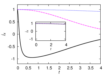
Figure 1: (color online) $j_{x}$ vs $t$ without a bath (upper dotted, blue), with an Ohmic bath but using a factorized initial state (dot-dashed, magenta), and with an Ohmic bath and including SBC effects (solid, black). $N=2000$, $\omega_{0}=0.1$, $G=0.001$, $\beta=1000$, and $\omega_{c}=10$ footnoteparameters . Inset shows the parallel results if $N=1$, where three lines become almost indistinguishable.

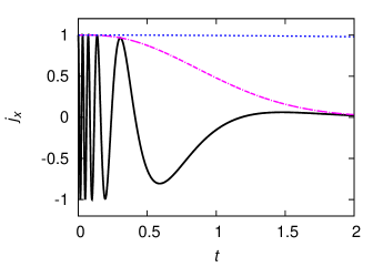
Figure 2: (color online) Same as in Fig. 1, but now with $N=20000$. The rapid oscillations in $j_{x}$ clearly demonstrate the amplification of SBC effects achieved by an increase in the number of particles.

In this section we turn to a concrete example for which we investigate the dynamics of a scaled observable $j_{x}\equiv 2\langle J_{x}\rangle/N$. At time zero, the system is projected onto the initial spin state $\left|\psi\right\rangle=e^{-i\frac{\pi}{2}J_{y}}\left|N/2\right\rangle$. Using the uncorrelated initial state in Eq. (5), we obtain

$$j_{x}=e^{-\gamma(t)t}\text{Re}\left[e^{i[\omega_{0}+\Delta(t)]t}X(t)\right],$$ (21)

with

$$X(t) = \frac{2}{N}\sum_{m}\frac{1}{2^{N}}e^{2imt\Delta(t)}$$ (22)

$$\times\ \sqrt{\binom{N}{\frac{N}{2}+m}\binom{N}{\frac{N}{2}+m+1}\left(\frac{N}{2}-m\right)\left(\frac{N}{2}+m+1\right)}.$$

Details can be found in Appendix D. By contrast, the true dynamics with the physical initial state in Eq. (4) gives

$$j_{x}=e^{-\gamma(t)t}\text{Re}\left[e^{i[\omega_{0}+\Delta(t)]t}X(t)F^{c}_{x}(t)\right],$$ (23)

with $F^{c}_{x}(t)\approx e^{iNG\omega_{c}t}$ at short times for an Ohmic spectrum defined above. In Fig. 1, we plot the time dependence of $j_{x}$ for $N=2000$, in the absence or presence of a bath with $G\ll 1$ (so that each individual two-level atom interacts with the bath very weakly VorrathChemPhys2004 ). For the shown time period in Fig. 1, $j_{x}$ in the absence of the bath hardly changes due to a finite $\omega_{0}$. In the presence of the bath but without including SBCs, $j_{x}$ stays positive but decreases at a faster rate due to the bath-assisted atom-atom interaction. With SBCs accounted for, completely different qualitative behavior of $j_{x}$ is observed: it rapidly changes from $1$ to $-1$ and then gradually returns to a value close to zero. Note that, as analyzed in theory, such rapid change in $j_{x}$ occurs before atom-atom indirect interaction (as captured by $\Delta(t)$) takes effect. The inset also shows the parallel results if $N=1$, with all other parameters unchanged. As expected from $G\ll 1$, in that case all lines are almost on top of each other and hence no SBC effect can be seen. Because the decoherence function $\gamma(t)$ is independent of $N$, the results in the inset also hint that decoherence for the $N=2000$ case is insignificant for the shown time scale. Therefore, SBCs impact on the dynamics long before the onset of decoherence.

To emphasize the role of $N$, in Fig. 2 we plot parallel results for $N=20000$. There SBCs induce more drastic oscillations in $j_{x}$, followed by slower oscillations as the time dependence of $F^{c}_{mn}(t)$ weakens. Clearly then, at short times an increasing number of atoms enhances the oscillation frequency in physical observables, thus amplifying the SBC effects.

IV Suppression of system-bath correlation effects by dynamical decoupling

In this section we discuss the implications of this work for DD, which is one main approach to quantum state protection LloydDD ; UhrigDD ; liuUDD . DD in single-spin systems has found enormous applications. It is therefore highly desirable to extend DD to systems describable by collective (large) spins $J_{x,y,z}$ adampra2012 ; largespin . We return to our pure-dephasing model introduced in Sec. II. Because the details of a bath spectrum is unknown in general, the precise form of the correction factor $F^{c}_{mn}(t)$ induced by SBCs or of the $\Delta(t)$-related phase factor due to bath-assisted atom-atom interaction is unavailable in general. It is tempting to wait for $F^{c}_{mn}(t)$ to saturate such that its time dependence is out of the picture. However, as indicated by our theory and shown in Fig. 2, before reaching that regime the bath assisted atom-atom interaction would have already changed the state. So in order to protect or store a given many-body state, the time dependence of $F^{c}_{mn}(t)$ and $\Delta(t)$ must be suppressed. In general the task of DD becomes three-fold: to suppress the decoherence factor $\gamma(t)$, the $\Delta(t)$-related phase factor, and the correction factor $F^{c}_{mn}(t)$. For large $N$, it is found that DD control pulses need to first compete with the correlated-induced time scale $t_{c}\varpropto 1/N$.

Consider now $N_{d}$ instantaneous $\pi$-pulses of $J_{x}$ applied to our system at times $t_{l}$, with $1\leq l\leq N_{d}$. Upon application of one such pulse, one has, in the frame of the applied pulses, $J_{z}\rightarrow-J_{z}$. It is hence convenient to introduce the so-called switching function $f(t)$, with

$$f(t)=\sum_{l=1}^{N_{d}+1}(-1)^{l+1}\theta(t-t_{l-1})\theta(t_{l}-t),$$ (24)

where $\theta(t)$ is the Heaviside function. With the assistance of $f(t)$, one can still find the time dependence of $[\rho_{S}(t)]_{mn}$ or of an observable such as $j_{x}$ analytically, using the same technique as used in previous cases without DD pulses. Take $[\rho_{S}(t)]_{mn}$ under DD as an example. The general form of Eq. (II) still holds, but now with $\omega_{0}(t)$ changed to $\tilde{\omega}_{0}(t)$, $\Delta(t)$ changed to $\tilde{\Delta}(t)$, $\gamma(t)$ changed to $\tilde{\gamma}(t)$, and $F_{mn}^{c}(t)$ changed to $\tilde{F}^{c}_{mn}(t)$. Specifically, we find

$$\tilde{\omega}_{0} = \frac{\omega_{0}}{t}\int_{0}^{t}f(t^{\prime})dt^{\prime},$$

$$\tilde{\Delta}(t) = \sum_{k}\frac{4|g_{k}|^{2}}{t}\int_{0}^{t}dt_{1}\int_{0}^{t_{1}}dt_{2}f(t_{1})f(t_{2})\sin[\omega_{k}(t_{2}-t_{1})],$$

$$\tilde{\gamma}(t) = \sum_{k}4|g_{k}|^{2}\frac{|f(\omega_{k},t)|^{2}}{\omega_{k}^{2}t}\coth\left(\frac{\beta\omega_{k}}{2}\right),$$ (25)

and

$$\tilde{F}^{c}_{mn}(t)\approx e^{-i\left[N(n-m)\sum_{k}4|g_{k}|^{2}\text{Im}[f(\omega_{k},t)]/\omega_{k}^{2}\right]}.$$ (26)

Here

$$f(\omega_{k},t)=1+(-1)^{N_{d}+1}e^{i\omega_{k}t}+2\sum_{l=1}^{N_{d}}(-1)^{l}e^{i\omega_{k}t_{l}}$$ (27)

is determined by $f(t)$ via the following relation

$$f(\omega_{k},t)=-i\omega_{k}\int_{0}^{t}dt^{\prime}e^{i\omega_{k}t^{\prime}}f(t^{\prime}).$$ (28)

With these explicit results, effects of DD pulses on the dynamics with SBC effects can be examined in detail. Of particular interest is $\tilde{F}^{c}_{mn}(t)$ because it is indicative of the impact of an applied DD sequence on SBC effects at early times.

In Fig.  3 we illustrate the effect of applying DD pulses for $N=20000$ for a final time $t=0.1$. We first investigate the usefulness of equidistance control pulses (bang-bang control) with a pulse interval $\tau$ LloydDD . Note first that if we neglect SBCs, then there would be no need to apply any DD pulses because the evolution of $j_{x}$ is negligible for the considered period. With SBCs accounted for, an application of $N_{d}=4$ pulses with $\tau=0.02$ is found to be insufficient for state protection. Indeed, for the system parameters used we find $t_{c}=(GN\omega_{c})^{-1}=0.005$, which is far smaller than $\tau=0.02$. To compete with $t_{c}$, we then use $\tau=0.002<t_{c}$, for which the evolution is successfully frozen (see Fig. 3).

To avoid the need of a high pulse repetition rate, we next consider the celebrated, more effective, Uhrig’s dynamical decoupling (UDD) sequence UhrigDD ; liuUDD with unequal pulse intervals, where the pulse timings are given by $t_{j}=t\sin^{2}\left(\frac{j\pi}{2N_{p}+2}\right)$. Dramatically, via only $N_{d}=4$ UDD pulses, the $j_{x}$ value at the final time $t=0.1$ is already recovered to its initial value. A careful look into the above expression for $\tilde{F}^{c}_{mn}(t)$ explains why this is so. The original motivation of a UDD sequence is to suppress the decoherence function $\gamma(t)$ by minimizing $|f(\omega_{k},t)|$ to its $N_{d}$-th order in time. So by construction, the time evolution of $\tilde{F}^{c}_{mn}(t)$ is also optimally suppressed by UDD because a minimized $|f(\omega_{k},t)|$ automatically yields a minimized $\text{Im}[f(\omega_{k},t)]$ that enters into $\tilde{F}^{c}_{mn}(t)$ in Eq. (26). That is, here the correction factor $\tilde{F}_{mn}^{c}(t)$ is already optimally suppressed for an unknown spectrum with an exponential cutoff. Additional computational studies indicate that the $\tilde{\Delta}(t)$ term may be also well suppressed by DD pulses, though this is not of interest here as our main concern is to suppress SBC before bath-assisted atom-atom interaction has any considerable effect on the dynamics. Our conclusions are as follows. In locking a many-body state in our model here, the previously unknown time scale $t_{c}$ induced by SBC calls for the use of DD control pulses long before decoherence and bath-assisted atom-atom interaction becomes important, with a UDD sequence found to be an optimized choice (assuming the detailed form of the bath spectrum is not available).

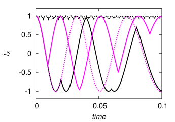
Figure 3: (color online) $j_{x}$ vs time with SBC effects and under bang-bang control pulses, for $\tau=0.02$ (solid, black) or $\tau=0.002$ (dotted, black). The parallel results without any control pulses (dotted, magenta) and with four UDD pulses (solid, magenta) are also shown. Parameters are the same as in Fig. 2, with the final time chosen as $t=0.1$.

V summary

In summary, because SBC effects are amplified by the number of particles in a many-body system, they can be important even when each individual particle interacts with the bath weakly. Interestingly, though SBC effects originate from system-bath interaction in the long past, they may still be suppressed by dynamical decoupling so that a prepared many-body state is well protected. Nevertheless, reaching this goal calls for more effective control pulses applied within a shorter time scale. Our results should also be of interest to other subtopics in open many-body systems by considering SBC effects neglected before.

VI Acknowledgment

We would like to thank Derek Ho for insightful discussions.

Appendix A Exact unitary evolution operator

The dynamics for our model described by Eqs. (1)-(3) can be exactly solved if $\delta=0$. Purely for convenience we also assume $\chi=0$. We first transform to the interaction picture. In this picture, the Hamiltonian becomes

$$H_{I}(t) =e^{i(H_{S}+H_{B})t}H_{\text{int}}e^{-i(H_{S}+H_{B})t},$$

$$=2J_{z}\sum_{k}(g_{k}^{*}b_{k}e^{-i\omega_{k}t}+g_{k}b_{k}^{\dagger}e^{i\omega_{k}t}).$$ (29)

Similar to the treatment in Ref. KurizkiPRL2011 , we next find the time evolution operator $U_{I}(t)$ corresponding to $H_{I}(t)$. The Magnus expansion Magnus1954 tells us that

$$U_{I}(t)=\exp\left[\sum_{i=1}^{\infty}A_{i}(t)\right],$$ (30)

where

$$A_{1}(t)=-i\int_{0}^{t}dt_{1}H_{I}(t_{1}),$$ (31)

$$A_{2}(t)=-\frac{1}{2}\int_{0}^{t}dt_{1}\int_{0}^{t_{1}}dt_{2}[H_{I}(t_{1}),H_{I}(t_{2})].$$ (32)

It is straightforward to find

$$A_{1} =-i\int_{0}^{t}dt_{1}H_{I}(t_{1}),$$

$$=J_{z}\sum_{k}(b_{k}^{\dagger}\alpha_{k}(t)-b_{k}\alpha_{k}^{*}(t)),$$ (33)

where

$$\alpha_{k}(t)=\frac{2g_{k}(1-e^{i\omega_{k}t})}{\omega_{k}}.$$ (34)

Further using

$$[H_{I}(t_{1}),H_{I}(t_{2})]=-8iJ_{z}^{2}\sum_{k}|g_{k}|^{2}\sin[\omega_{k}(t_{1}-t_{2})],$$ (35)

we obtain

$$A_{2} =\frac{1}{2}\int_{0}^{t}dt_{1}\int_{0}^{t_{1}}dt_{2}8iJ_{z}^{2}\sum_{k}|g_{k}|^{2}\sin[\omega_{k}(t_{1}-t_{2})],$$

$$=-iJ_{z}^{2}t\Delta(t),$$ (36)

where

$$\Delta(t)\equiv\frac{1}{t}\sum_{k}4|g_{k}|^{2}\frac{[\sin(\omega_{k}t)-\omega_{k}t]}{\omega_{k}^{2}}.$$ (37)

Since this is a c-number, the higher order terms in the Magnus expansion are all zero. The exact unitary time evolution operator is hence found, i.e.,

$$U(t)=e^{-i\omega_{0}J_{z}t}e^{-iH_{B}t}U_{I}(t),$$ (38)

where

$$U_{I}(t)=\exp\{J_{z}\sum_{k}[b_{k}^{\dagger}\alpha_{k}(t)-b_{k}\alpha_{k}^{*}(t)]-iJ_{z}^{2}t\Delta(t)\}.$$ (39)

For later calculations, let us first consider the reduced density operator of the system

$$\rho_{S}(t)=\text{Tr}_{B}[U(t)\rho(0)U^{\dagger}(t)],$$ (40)

where $\rho(0)$ is the density operator of the system and the bath as a whole. We find it useful to write the reduced density operator of the system in terms of the standard $J_{z}$ basis as

$$[\rho_{S}(t)]_{mn}=\text{Tr}_{S,B}[U(t)\rho(0)U^{\dagger}(t)P_{nm}].$$ (41)

Here $P_{nm}\equiv\left|n\right\rangle\left\langle m\right|$, $\left|n\right\rangle$ being the eigenstate of $J_{z}$ with eigenvalue $n$. Introducing the Heisenberg picture operator $P_{nm}(t)$ as $U^{\dagger}(t)P_{nm}U(t)$, we have

$$[\rho_{S}(t)]_{mn}=\text{Tr}_{S,B}[P_{nm}(t)\rho(0)].$$ (42)

Calculations of the explicit form of $P_{nm}(t)$ are straightforward because the time evolution operator $U(t)$ is already found. In particular, we obtain

$$P_{nm}(t)=e^{-i\omega_{0}t(m-n)}e^{-i\Delta(t)t(m^{2}-n^{2})}e^{-R_{nm}(t)}P_{nm},$$ (43)

where

$$R_{nm}(t)=(n-m)\sum_{k}[b_{k}^{\dagger}\alpha_{k}(t)-b_{k}\alpha_{k}^{*}(t)].$$ (44)

It follows that

$$[\rho_{S}(t)]_{mn}=e^{-i\omega_{0}t(m-n)}e^{-i\Delta(t)t(m^{2}-n^{2})}\text{Tr}_{S,B}[e^{-R_{nm}(t)}P_{nm}\rho(0)].$$ (45)

This is a general result because it applies to an arbitrary initial density $\rho(0)$ (the unphysical state $\rho^{\text{dir}}(0)$ or the physical state with SBC accounted for).

Appendix B Dynamics with uncorrelated initial states

Here we consider unphysical decorrelated initial states, i.e.,

$$\rho^{\text{dir}}(0)=\rho_{S}(0)\otimes\rho_{B},$$ (46)

where $\rho_{B}=\frac{e^{-\beta H_{B}}}{Z_{B}}$ with $Z_{B}=\text{Tr}_{B}[e^{-\beta H_{B}}]$. Then,

$$[\rho_{S}(t)]_{mn}=[\rho_{S}(0)]_{mn}e^{-i\omega_{0}(m-n)t}e^{-i\Delta(t)(m^{2}-n^{2})t}\text{Tr}_{B}[e^{-R_{nm}(t)}\rho_{B}].$$ (47)

We now simplify $\text{Tr}_{B}[e^{-R_{nm}(t)}\rho_{B}]=\langle e^{-R_{nm}(t)}\rangle$, where the average is taken with respect to the thermal bath state at equilibirum. Although this is a standard result, for self-completeness, we explain the steps in detail. Since the modes are independent of each other, we can write

$$\langle e^{-R_{nm}(t)}\rangle=\prod_{k}\langle e^{-(n-m)[b_{k}^{\dagger}\alpha_{k}(t)-b_{k}\alpha_{k}^{*}(t)]}\rangle.$$ (48)

For an operator $A$ which is a linear combination of creation and annihilation operators, we have $\langle e^{A}\rangle=e^{\langle A^{2}\rangle/2}$. Using this identity, we have

$$\langle e^{-R_{nm}(t)}\rangle =\prod_{k}\exp\left[-\frac{1}{2}(n-m)^{2}|\alpha_{k}(t)|^{2}\langle b_{k}^{\dagger}b_{k}+b_{k}b_{k}^{\dagger}\rangle\right]$$

$$=\prod_{k}\exp\left[-\frac{1}{2}(n-m)^{2}|\alpha_{k}(t)|^{2}\langle 2n_{k}+1\rangle\right].$$ (49)

Further using the definition of $\alpha_{k}(t)$ and the Bose-Einstein distribution, we find that

$$\text{Tr}_{B}[e^{-R_{nm}(t)}\rho_{B}]=\exp\left[-\sum_{k}(m-n)^{2}4|g_{k}|^{2}\frac{[1-\cos(\omega_{k}t)]}{\omega_{k}^{2}}\coth\left(\frac{\beta\omega_{k}}{2}\right)\right].$$

This then yields

$$[\rho_{S}(t)]_{mn}=[\rho_{S}(0)]_{mn}e^{-i\omega_{0}(m-n)t}e^{-i\Delta(t)(m^{2}-n^{2})t}e^{-\gamma(t)(m-n)^{2}t},$$ (50)

with

$$\gamma(t)=\frac{1}{t}\sum_{k}4|g_{k}|^{2}\frac{(1-\cos(\omega_{k}t))}{\omega_{k}^{2}}\coth\left(\frac{\beta\omega_{k}}{2}\right).$$ (51)

The factor $e^{-\gamma(t)(m-n)^{2}t}$ describes decoherence and the factor $e^{-i\Delta(t)(m^{2}-n^{2})t}$ describes the indirect atom-atom interaction induced by the common bath.

Appendix C Dynamics with system-bath-correlated initial states

Here we consider (physical) correlated initial states of the form

$$\rho(0)=\frac{1}{Z}\sum_{r}\Omega_{r}e^{-\beta H_{\text{total}}}\Omega_{r}^{\dagger},$$ (52)

with

$$Z=\text{Tr}_{S,B}\left[\sum_{r}\Omega_{r}e^{-\beta H_{\text{total}}}\Omega_{r}^{\dagger}\right].$$ (53)

The $\Omega_{r}$ operators above are assumed to be acting on the system only and their explicit forms will be specified later. To solve for the dynamics starting from such an initial state, we may use a polaron transformation technique, generalizing the results of Ref. MorozovPRA2012 from a single spin to many spins, or we may use displaced harmonic oscillator modes. The latter method is used below since it is physically more transparent.

We first simplify $Z$. By introducing a completeness relation, we find that

$$Z =\sum_{r}\sum_{l}\text{Tr}_{S,B}[\Omega_{r}e^{-\beta H_{\text{total}}}\left|l\right\rangle\left\langle l\right|\Omega_{r}^{\dagger}],$$

$$=\sum_{r}\sum_{l}e^{-\beta\omega_{0}l}\left\langle l|\Omega_{r}^{\dagger}\Omega_{r}|l\right\rangle\text{Tr}_{B}[e^{-\beta H_{B}^{(l)}}],$$ (54)

where we have defined

$$H_{B}^{(l)}=H_{B}+2l\sum_{k}(g_{k}^{*}b_{k}+g_{k}b_{k}^{\dagger}).$$ (55)

Using the displaced harmonic oscillator modes,

$$B_{k,l}=b_{k}+\frac{2lg_{k}}{\omega_{k}},$$ (56)

$$B_{k,l}^{\dagger}=b_{k}^{\dagger}+\frac{2lg_{k}^{*}}{\omega_{k}}.$$ (57)

we find

$$Z=\sum_{r}\sum_{l}e^{-\beta\omega_{0}l}\left\langle l|\Omega_{r}^{\dagger}\Omega_{r}|l\right\rangle e^{\beta l^{2}\mathcal{C}}Z_{B},$$ (58)

where $\mathcal{C}=\sum_{k}\frac{4|g_{k}|^{2}}{\omega_{k}}$, and in this case $Z_{B}=\text{Tr}_{B}[e^{-\beta\sum_{k}\omega_{k}B_{k,l}^{\dagger}B_{k,l}}]$.

We now substitute Eq. (52) in Eq. (45) and again introduce a completeness relation. To proceeed, $\text{Tr}_{B}[e^{-R_{nm}(t)}e^{-\beta H_{B}^{(l)}}]$ needs to be simplified. As before, this can be done using displaced oscillator modes. It is straightforward to show that

$$R_{nm}(t)=(n-m)\sum_{k}[\alpha_{k}(t)B_{k,l}^{\dagger}-\alpha_{k}^{*}(t)B_{k,l}]+i\Phi_{nm}^{(l)}(t),$$ (59)

where

$$\Phi_{nm}^{(l)} = 2(n-m)l\Phi(t),$$ (60)

$$\Phi(t) = \sum_{k}\frac{4|g_{k}|^{2}}{\omega_{k}^{2}}\sin(\omega_{k}t).$$ (61)

We then find that

$$\text{Tr}_{B}[e^{-R_{nm}(t)}e^{-\beta H_{B}^{(l)}}]=e^{-i\Phi_{nm}^{(l)}(t)}e^{\beta l^{2}\mathcal{C}}Z_{B}e^{-\gamma(t)(m-n)^{2}t},$$ (62)

which leads to

$$[\rho_{S}(t)]_{mn} = e^{-i\omega_{0}(m-n)t}e^{-i\Delta(t)(m^{2}-n^{2})t}e^{-\gamma(t)(m-n)^{2}t}$$ (63)

$$\times\ \dfrac{\sum_{r}\sum_{l}\left(\left\langle l|\Omega_{r}^{\dagger}P_{nm}\Omega_{r}|l\right\rangle e^{-i\Phi_{nm}^{(l)}(t)}e^{-\beta\omega_{0}l}e^{\beta l^{2}\mathcal{C}}\right)}{\sum_{r}\sum_{l}\left(\left\langle l|\Omega_{r}^{\dagger}\Omega_{r}|l\right\rangle e^{-\beta\omega_{0}l}e^{\beta l^{2}\mathcal{C}}\right)}.$$

Noting that

$$[\rho_{S}(0)]_{mn}=\dfrac{\sum_{r}\sum_{l}\left(\left\langle l|\Omega_{r}^{\dagger}P_{nm}\Omega_{r}|l\right\rangle e^{-\beta\omega_{0}l}e^{\beta l^{2}\mathcal{C}}\right)}{\sum_{r}\sum_{l}\left(\left\langle l|\Omega_{r}^{\dagger}\Omega_{r}|l\right\rangle e^{-\beta\omega_{0}l}e^{\beta l^{2}\mathcal{C}}\right)},$$ (64)

one finally arrives at

$$[\rho_{S}(t)]_{mn} =[\rho_{S}(0)]_{mn}e^{-i\omega_{0}(m-n)t}e^{-i\Delta(t)(m^{2}-n^{2})t}e^{-\gamma(t)(m-n)^{2}t}$$

$$\times\dfrac{\sum_{r}\sum_{l}\left(\left\langle l|\Omega_{r}^{\dagger}P_{nm}\Omega_{r}|l\right\rangle e^{-i\Phi_{nm}^{(l)}(t)}e^{-\beta\omega_{0}l}e^{\beta l^{2}\mathcal{C}}\right)}{\sum_{r}\sum_{l}\left(\left\langle l|\Omega_{r}^{\dagger}P_{nm}\Omega_{r}|l\right\rangle e^{-\beta\omega_{0}l}e^{\beta l^{2}\mathcal{C}}\right)}.$$ (65)

C.1 State preparation via projective measurement

In this case,

$$\rho(0)=\frac{1}{Z}P_{\psi}e^{-\beta H_{\text{total}}}P_{\psi}$$ (66)

with $P_{\psi}=\left|\psi\right\rangle\left\langle\psi\right|$. Using our general results above we obtain

$$[\rho_{S}(t)]_{mn} = [\rho_{S}(0)]_{mn}e^{-i\omega_{0}(m-n)t}e^{-i\Delta(t)(m^{2}-n^{2})t}e^{-\gamma(t)(m-n)^{2}t}$$ (67)

$$\times\ \dfrac{\sum_{l}\left(|\langle l|\psi\rangle|^{2}e^{-i\Phi_{nm}^{(l)}(t)}e^{-\beta\omega_{0}l}e^{\beta l^{2}\mathcal{C}}\right)}{\sum_{l}\left(|\langle l|\psi\rangle|^{2}e^{-\beta\omega_{0}l}e^{\beta l^{2}\mathcal{C}}\right)}.$$

This can be rewritten as

$$[\rho_{S}(t)]_{mn}=[\rho_{S}(0)]_{mn}e^{-i\omega_{0}(m-n)t}e^{-i\Delta(t)(m^{2}-n^{2})t}e^{-\gamma(t)(m-n)^{2}t}F_{mn}^{c}(t),$$ (68)

where $F_{mn}^{c}(t)$ is already given in the main text.

C.2 State preparation via unitary operations

Alternatively, instead of performing a projective measurement on the system, we may first cool the system and the bath to a desired low temperature. We then perform a unitary operation on the system to approximately arrive at some initial state. In general, initial state of the system and the bath prepared in this manner can be written as

$$\rho(0)=\frac{1}{Z}\Omega e^{-\beta H_{\text{total}}}\Omega^{\dagger},$$ (69)

with $\Omega$ being a unitary preparation operator acting on the system Hilbert space. We then have

$$[\rho_{S}(t)]_{mn} = [\rho_{S}(0)]_{mn}e^{-i\omega_{0}(m-n)t}e^{-i\Delta(t)(m^{2}-n^{2})t}e^{-\gamma(t)(m-n)^{2}t}$$ (70)

$$\times\ \dfrac{\sum_{l}\left(\left\langle l|\Omega^{\dagger}|n\right\rangle\left\langle m|\Omega|l\right\rangle e^{-i\Phi_{nm}^{(l)}(t)}e^{-\beta\omega_{0}l}e^{\beta l^{2}\mathcal{C}}\right)}{\sum_{l}\left(\left\langle l|\Omega^{\dagger}|n\right\rangle\left\langle m|\Omega|l\right\rangle e^{-\beta\omega_{0}l}e^{\beta l^{2}\mathcal{C}}\right)}.$$

This can be rewritten as

$$[\rho_{S}(t)]_{mn}=[\rho_{S}(0)]_{mn}e^{-i\omega_{0}(m-n)t}e^{-i\Delta(t)(m^{2}-n^{2})t}e^{-\gamma(t)(m-n)^{2}t}\left[\sum_{l}\mu^{(l)}_{nm}e^{-i\Phi_{nm}^{(l)}(t)}\right],$$ (71)

with

$$\mu^{(l)}_{nm}=\dfrac{\left\langle l|\Omega^{\dagger}|n\right\rangle\left\langle m|\Omega|l\right\rangle e^{-\beta\omega_{0}l}e^{\beta l^{2}\mathcal{C}}}{\sum_{l}\left(\left\langle l|\Omega^{\dagger}|n\right\rangle\left\langle m|\Omega|l\right\rangle e^{-\beta\omega_{0}l}e^{\beta l^{2}\mathcal{C}}\right)}.$$ (72)

Note that $\mu^{(l)}_{nm}$ need not be real here (nevertheless, by its definition only, we still have $\sum_{l}\mu^{(l)}_{nm}=1$).

Appendix D Calculating observables

To evaluate physical observables using the system’s reduced density operator, let us first evaluate the functions $\gamma(t)$, $\Phi(t)$, $\mathcal{C}$ and $\Delta(t)$. As usual, we take the continuum limit of the bath modes, whereby the summations over the bath modes are replaced by integrals via the rule

$$\sum_{k}4|g_{k}|^{2}C(\omega_{k})=\int_{0}^{\infty}d\omega J(\omega)C(\omega),$$ (73)

with $J(\omega)$ being the spectral density. For this work, we choose Ohmic spectral density, that is,

$$J(\omega)=G\omega e^{-\omega/\omega_{c}}.$$ (74)

We can then evaluate the integrals as MorozovPRA2012 ,

$$\mathcal{C}=G\omega_{c},$$ (75)

$$\Phi(t)=G\tan^{-1}(\omega_{c}t),$$ (76)

and

$$\gamma(t) =\gamma_{\text{vac}}(t)+\gamma_{\text{th}}(t),$$ (77)

$$\gamma_{\text{vac}}(t) =\frac{G}{2t}\text{ln}(1+\omega_{c}^{2}t^{2}),$$ (78)

$$\gamma_{\text{th}}(t) =\frac{2G}{t}[\text{ln}\Gamma(1+\frac{1}{\beta\omega_{c}})-\frac{1}{2}\text{ln}|\Gamma(1+\frac{1}{\beta\omega_{c}}+\frac{it}{\beta})|^{2}],$$ (79)

$$\Delta(t) =\frac{1}{t}(\Phi(t)-\mathcal{C}t).$$ (80)

Expressions for sub-Ohmic and super-Ohmic spectral densities can also be found in Ref. MorozovPRA2012 that treated a single two-level system in a bath.

To evaluate the expectation value of $J_{x}$, we first calculate $\langle J_{+}(t)\rangle$, where $J_{+}=J_{x}+iJ_{y}$ is the standard angular momentum ladder operator. Note first that

$$\langle J_{+}(t)\rangle=\sum_{mn}\rho_{mn}(t)(J_{+})_{nm}.$$ (81)

Using

$$\left\langle n|J_{+}|m\right\rangle=\sqrt{\left(\frac{N}{2}-m\right)\left(\frac{N}{2}+m+1\right)}\,\delta_{n,m+1}.$$ (82)

one obtains

$$\left\langle J_{+}(t)\right\rangle=\sum_{m}\rho_{m,m+1}(t)\sqrt{\left(\frac{N}{2}-m\right)\left(\frac{N}{2}+m+1\right)}.$$ (83)

We then have

$$j_{x}\equiv\frac{2}{N}\left\langle J_{+}(t)\right\rangle=e^{i\omega_{0}t}e^{i\Delta(t)t}e^{-t\gamma(t)}X(t)F_{x}^{c}(t),$$ (84)

where

$$X(t) =\frac{2}{N}\sum_{m}[\rho_{S}(0)]_{m,m+1}e^{2i\Delta(t)mt}\sqrt{\left(\frac{N}{2}-m\right)\left(\frac{N}{2}+m+1\right)},$$ (85)

$$F_{x}^{c}(t) =\sum_{l}p_{l}e^{-2il\Phi(t)}.$$ (86)

For the initial state $\left|\psi\right\rangle=e^{-i\frac{\pi}{2}J_{y}}\left|\frac{N}{2}\right\rangle$ prepared by a projective measurement, it is an eigenstate of $J_{x}$ with eigenvalue $\frac{N}{2}$. Then,

$$[\rho_{S}(0)]_{m,m+1}=\left\langle m|e^{-i\frac{\pi}{2}J_{y}}|N/2\right\rangle\left\langle N/2|e^{i\frac{\pi}{2}J_{y}}|m+1\right\rangle.$$ (87)

Note that $\left\langle m|e^{-i\alpha J_{y}}|m^{\prime}\right\rangle$ is a Wigner “d-matrix” element. Using the Wigner formula, we obtain

$$\left\langle m|e^{-i\frac{\pi}{2}J_{y}}|N/2\right\rangle=\frac{1}{2^{\frac{N}{2}}}\sqrt{\binom{N}{\frac{N}{2}+m}}.$$ (88)

Then,

$$[\rho_{S}(0)]_{m,m+1}=\frac{1}{2^{N}}\sqrt{\binom{N}{\frac{N}{2}+m}\binom{N}{\frac{N}{2}+m+1}},$$ (89)

from which we have

$$X(t)=\frac{2}{N}\sum_{m}\frac{1}{2^{N}}e^{2imt\Delta(t)}\sqrt{\binom{N}{\frac{N}{2}+m}\binom{N}{\frac{N}{2}+m+1}\left(\frac{N}{2}-m\right)\left(\frac{N}{2}+m+1\right)},$$ (90)

which is also given in the main text. The observable $j_{x}$ is then given by

$$j_{x}=e^{-t\gamma(t)}\text{Re}\left[e^{i[\omega_{0}+\Delta(t)]t}X(t)F_{x}^{c}(t)\right].$$ (91)

As to $F_{x}^{c}(t)$ [see Eq. (86)] that involves the summation over $p_{l}$, it can be seen that for large $N$, $F_{x}^{c}(t)\approx e^{iN\Phi(t)}$. That is, due to the exponential factors $e^{-\beta\omega_{0}l}$ and $e^{\beta l^{2}\mathcal{C}}$, only the $l=-N/2$ term makes a dominating contribution if $N\gg 1$.

We now comment on what happens if, instead of a projective measurement, we use a unitary operation. It can be easily shown that

$$[\rho_{S}(0)]_{mn}\varpropto\sum_{l}\left\langle m|\Omega|l\right\rangle\left\langle l|\Omega^{\dagger}|n\right\rangle e^{-\beta\omega_{0}l}e^{\beta l^{2}\mathcal{C}}.$$ (92)

Once again the term with $l=-\frac{N}{2}$ dominates, so that

$$[\rho_{S}(0)]_{mn}\approx\left\langle m|\Omega|-N/2\right\rangle\left\langle-N/2|\Omega^{\dagger}|n\right\rangle$$ (93)

By setting the unitary operator $\Omega$ to be $e^{i\frac{\pi}{2}J_{y}}$, we see that our initial state is approximately the same as in the case of state preparation via projective measurement, with $F_{x}^{c}(t)\approx e^{iN\Phi(t)}$ for large $N$. As such, for large $N$ the $j_{x}$ dynamics are very much the same for the above-mentioned two realizations of initial state preparation.

References

• (1) H.-P. Breuer and F. Petruccione, The Theory of Open Quantum Systems (Oxford University Press, Oxford, 2007).
• (2) E. Pollak, J. Shao and D. H. Zhang, Phys. Rev. E 77, 021107 (2008).
• (3) P. Pechukas, Phys. Rev. Lett.  73, 1060 (1994).
• (4) A. Royer, Phys. Rev. Lett.  77, 3272 (1996).
• (5) M. Campisi, P. Talkner, and P. Hänggi, Phys. Rev. Lett.  102, 210401 (2009).
• (6) A. G. Dijkstra and Y. Tanimura, Phys. Rev. Lett.  104, 250401 (2010).
• (7) C. K. Lee, J. S.  Cao, and J. B. Gong, Phys. Rev. E 86, 021109 (2012).
• (8) V. Hakim and V. Ambegaokar, Phys. Rev. A 32, 423 (1985).
• (9) F. Haake and R. Reibold, Phys. Rev. A 32, 2462 (1985).
• (10) H. Grabert, P. Schramm and G-L. Ingold, Phys. Rep. 168, 115 (1988).
• (11) C. M. Smith and A. O. Caldeira, Phys. Rev. A 41, 3103 (1990).
• (12) R. Karrlein and H. Grabert, Phys. Rev. E 55, 153 (1997).
• (13) L. D. Romero and J. P. Paz, Phys. Rev. A 55, 4070 (1997).
• (14) E. Lutz, Phys. Rev. A 67, 022109 (2003).
• (15) S. Banerjee and R. Ghosh, Phys. Rev. E 67, 056120 (2003).
• (16) N. G. van Kampen, J. Stat. Phys. 115, 1057 (2004).
• (17) M. Ban, Phys. Rev. A 80, 064103 (2009).
• (18) C. Uchiyama and M. Aihara, Phys. Rev. A 82, 044104 (2010); C. Uchiyama, Phys. Rev. A 85, 052104 (2012).
• (19) A. Smirne, H-P. Breuer, J. Piilo and B. Vacchini, Phys. Rev. A 82, 062114 (2010).
• (20) J. Dajka and J. Luczka, Phys. Rev. A 82, 012341 (2010); J. Dajka, J. Luczka and P. Hänggi, Phys. Rev. A 84, 032120 (2011).
• (21) H-T. Tan and W-M. Zhang, Phys. Rev. A 83, 032102 (2011).
• (22) V. G. Morozov, S. Mathey and G. Ropke, Phys. Rev. A 85, 022101 (2012).
• (23) W. G. Wang, L. W. He, and J. B. Gong, Phys. Rev. Lett.  108, 070403 (2012).
• (24) Y. J. Zhang, X-B. Zou, Y-J. Xia and G-C. Guo, Phys. Rev. A 82, 022108 (2010).
• (25) R. H. Dicke, Phys. Rev. 93, 99 (1954).
• (26) T. Vorrath, T. Brandes and B. Kramer, Chem. Phys. 296, 295 (2004).
• (27) T. Vorrath and T. Brandes, Phys. Rev. Lett.  95, 070402 (2005).
• (28) N. Bar-Gill, D. D. B. Rao and G. Kurizki, Phys. Rev. Lett.  107, 010404 (2011).
• (29) U. Weiss, Quantum Dissipative Systems (World Scientific, Singapore, 2008).
• (30) Assuming that intermode transitions dominate, we perform a unitary transformation of the Hamiltonian to find that these parameters correspond to the experimentally realizable values of $\omega_{0}=2\pi\times 1\,\text{kHz}$ and temperature in the nanokelvin regime [see C. Gross et al., Nature (London) 464, 08919 (2010) and M. Lapert et al., Phys. Rev. A 85, 023611 (2012)]. One time unit here then corresponds to approximately $16\,\mu s$.
• (31) L. Viola and S. Lloyd, Phys. Rev. A 58, 2733 (1998); L. Viola, S. Lloyd and E. Knill, Phys. Rev. Lett.  83, 4888 (1999).
• (32) G. S. Uhrig, Phys. Rev. Lett.  98, 100504 (2007).
• (33) W. Yang and R. B. Liu, Phys. Rev. Lett.  101, 180403 (2008).
• (34) A. Z. Chaudhry and J. B. Gong, Phys. Rev. A 86, 012311 (2012).
• (35) M. Koschorreck, M. Napolitano, B. Dubost and M. W. Mitchell, Phys. Rev. Lett.  105, 093602 (2010).
• (36) W. Magnus, Commun. Pure Appl. Math 7, 649 (1954).