Solvation of Complex Surfaces via Molecular Density Functional Theory

Abstract

We show that classical molecular density functional theory (MDFT), here in the homogeneous reference fluid approximation in which the functional is inferred from the properties of the bulk solvent, is a powerful new tool to study, at a fully molecular level, the solvation of complex surfaces and interfaces by polar solvents. This implicit solvent method allows for the determination of structural, orientational and energetic solvation properties that are on a par with all-atom molecular simulations performed for the same system, while reducing the computer time by two orders of magnitude. This is illustrated by the study of an atomistically-resolved clay surface composed of over a thousand atoms wetted by a molecular dipolar solvent. The high numerical efficiency of the method is exploited to carry a systematic analysis of the electrostatic and non-electrostatic components of the surface-solvent interaction within the popular CLAYFF force field. Solvent energetics and structure are found to depend weakly upon the atomic charges distribution of the clay surface, even for a rather polar solvent. We conclude on the consequences of such findings for force-field development.

I Introduction

Liquids at solid-liquid interfaces behave differently from bulk liquids. Interfacial phenomena play key roles in various applications like, for instance, heterogeneous catalysis, electrochemistry, adsorption and transport in porous media. It is our goal to improve the description of such interfaces at the microscopic scale.

Experimentally, specific techniques have been developed, such as the vibrational sum frequency spectroscopy Richmond (2002) or quasi-elastic neutron scattering techniques Marry et al. (2011), that now give access to information on the structural and dynamic properties of the liquid on few molecular layers on top of the surface. At these scales, theoretical modeling can clarify experimental observations by linking them to atomistic phenomena. For instance, Rotenberg et al. Rotenberg, Patel, and Chandler (2011) showed by molecular simulations that wetting properties of talc surfaces, that behave as hydrophilic or hydrophobic depending on the relative humidity, are a consequence of the competition between surface-solvent adhesion, favorable entropy in the gas phase and molecular cohesion in the liquid phase.

This kind of theoretical modeling is typically based on molecular dynamics (MD) or Monte Carlo simulations where each atom is considered individually. For systems that are intrinsically multiscale, e.g. porous media, one has to deal with thousands of atoms. At this point, numerical heaviness becomes critical and hinders systematic studies. To overcome this difficulty, various mesoscale models have been proposed, that are less computationally demanding. One can for instance forget the molecular nature of the solvent to only account for a Polarizable Continuum Medium (PCM) Leszczynski (1999); Tomasi, Cammi, and Mennucci (1999); Tomasi, Mennucci, and Cammi (2005), or simplify it to a hard sphere, with or without dipole Biben, Hansen, and Rosenfeld (1998); Dzubiella and Hansen (2004); Oleksy and Hansen (2010). Coarse-grained strategies have also been successfully applied to solid-liquid interfaces Jardat et al. (2009); Jardat, Hribar-Lee, and Vlachy (2012). While these methods and others proved efficient on a panel of problems, the applicability of their underlying approximation to an unknown system remains to be carefully and systematically checked.

In the second half of the last century, liquid state theories Gray and Gubbins (1984); Hansen and McDonald (2006) like the classical density functional theory (DFT) Evans (1979, 1992); Wu and Li (2007) have blossomed. Classical DFT, like other methods such as integral equations or classical field theories have shown to give thermodynamic and structural results comparable to all-atom simulations at attractive numerical cost, but they have for now been limited to highly symmetric systems, bulk fluids or simple model interfaces, e.g. hard and soft walls. A current challenge lies in the development of three-dimensional theories and implementations to describe molecular liquids, solutions, mixtures, in complex environments such as biomolecular media or atomically-resolved surfaces and interfaces. Recent developments in this direction use lattice field Azuara et al. (2006, 2008), or Gaussian field Varilly, Patel, and Chandler (2011) theoretical approaches, or the 3D reference interaction site model (3D-RISM) Beglov and Roux (1997); F. Hirata (2003); Kloss, Heil, and Kast (2008); Kloss and Kast (2008); Kovalenko and Hirata (1998); Yoshida et al. (2009), an appealing integral equation theory that has proven recently to be applicable to, e.g., structure prediction in complex biomolecular systems. Integral equations are, however, restricted by the choice of a closure relation (typically HyperNetted Chain (HNC), Percus-Yevick Percus and Yevick (1958), or Kovalenko-Hirata Kovalenko and Hirata (1998) approximation), and despite their great potential, they remain difficult to control and improve, and can prove difficult to converge.

Recently, a molecular density functional theory (MDFT) approach to solvation has been introduced. MDF ; Ramirez and Borgis (2005); Ramirez, Mareschal, and Borgis (2005); Gendre, Ramirez, and Borgis (2009); Zhao et al. (2011); Borgis, Gendre, and Ramirez (2012); Levesque, Vuilleumier, and Borgis (2012) It relies on the definition of a free-energy functional depending on the full six-dimensional position and orientation solvent density. In the so-called homogeneous reference fluid (HRF) approximation, the (unknown) functional can be inferred from the properties of the bulk solvent. Compared to reference molecular dynamics calculations, such approximation was shown to be accurate for polar, non-protic fluids Gendre, Ramirez, and Borgis (2009); Zhao et al. (2011); Borgis, Gendre, and Ramirez (2012), but to require corrections for waterZhao et al. (2011); Zhao, Jin, and Wu (2011a); Levesque, Vuilleumier, and Borgis (2012); Zhao, Jin, and Wu (2011b). Until now, only simple three-dimensional solutes have been considered in this framework including ions and polarZhao et al. (2011); Borgis, Gendre, and Ramirez (2012) or apolar Levesque, Vuilleumier, and Borgis (2012) molecules. In ref. Borgis, Gendre, and Ramirez (2012), the authors have shown that the MDFT scheme was applicable to the computation of electron-transfer properties such as reaction free energies and solvent reorganization free energies. In this paper, we show how the most recent developments of the molecular density functional theory, described here in the homogeneous reference fluid approximation MDF (HRF-MDFT), can be implemented to study the solvation of a complex atomically-resolved clay surface, the pyrophyllite, that contains over a thousand atoms. In order to uncouple the difficulties intrinsic to the method to those due to the particular correlations in water, we restrict ourselves here to a generic model of dipolar solvent, the Stockmayer fluid – with eventually parameters adjusted to mimick a few properties of water.

In section II, we present the most recent developments in molecular density functional theory in the homogeneous reference fluid approximation. We also describe our reference molecular dynamics simulations and the system under investigation. In section III, we discuss the structural and orientational properties of the complex interface between the solid and the dipolar liquid. There, we compare HRF-MDFT with reference molecular dynamics results. Finally, in section III.3, we illustrate the possibilities offered by the method in terms of numerical efficiency to analyze the electrostatic and non-electrostatic components of the state-of-the-art force field for clays, CLAYFF Cygan, Liang, and Kalinichev (2004). We conclude on the consequences of our analysis on force field development.

II Methods and Model System

II.1 Molecular Density Functional Theory of Solvation

II.1.1 Theoretical Aspects

Recent developments of a molecular density functional theory (MDFT) unlocked the study of the solvation of three-dimensional molecular solutes in arbitrary solvents using classical density functional theory. In MDFT, the solvent is composed of rigid molecules and described in terms of a position and orientation density, ${\rho\left({\mathbf{r}},\Omega\right)}$. The solvation free energy is defined as the difference between the grand potential $\Phi[\rho]$ of a system that includes external perturbation (a solute) and inhomogeneous solvent, and the grand potential $\Phi[\rho_{0}]$ of the homogeneous solvent at density $\rho_{0}=n_{0}/8\pi^{2}$, where $n_{0}$ is the number density, and without external potential,

$$F[\rho]=\Phi\left[\rho\right]-\Phi[\rho_{0}],$$ (1)

where $\rho$ and $\rho_{0}$ are the position and orientation densities of the inhomogeneous and homogeneous solvent. Following the theoretical framework introduced by Evans Evans (1979, 1992); Wu and Li (2007), the density functional $F$ can be rewritten as the sum of an ideal contribution ($F_{id}$), an excess term ($F_{exc}$) and an external (solute) contribution ($F_{ext}$),

$$F[\rho]=F_{id}[\rho]+F_{ext}[\rho]+F_{exc}[\rho].$$ (2)

The ideal and external contributions $F_{id}$ and $F_{ext}$ can be formally and exactly expressed as

$$F_{id}[\rho] = k_{B}T\int d\mathbf{r}d\Omega[{\rho\left({\mathbf{r}},\Omega\right)}{\rm ln}\left(\frac{{\rho\left({\mathbf{r}},\Omega\right)}}{\rho_{0}}\right)$$ (4)

$$-{\rho\left({\mathbf{r}},\Omega\right)}+\rho_{0}],$$

$$F_{ext}[\rho] = \int d\mathbf{r}d\Omega\ V_{ext}(\mathbf{r},\Omega){\rho\left({\mathbf{r}},\Omega\right)},$$ (5)

where $k_{B}$ is the Boltzmann constant and $T$ the temperature. $V_{ext}$ is the sum of the electrostatic and Lennard-Jones interactions between the solute and one solvent molecule located at $\mathbf{r}$ with orientation $\Omega$:

$$V_{ext}(\mathbf{r},\Omega) = \sum_{j\in\text{solvent}}\{q_{j}\,V_{q}(\mathbf{r}_{j})$$ (6)

$$+\sum_{i\in\text{solute}}4\epsilon_{ij}\left[\left(\frac{\sigma_{ij}}{r_{ij}}\right)^{12}-\left(\frac{\sigma_{ij}}{r_{ij}}\right)^{6}\right]\}.$$

If $\mathbf{R}(\Omega)$ is the rotation matrix associated to $\Omega$ and $\mathbf{s}_{j}$ is the position of the solvent site $j$ in the molecular frame, then $\mathbf{r}_{j}=\mathbf{r}+\mathbf{R}(\Omega)\mathbf{s}_{j}$ denotes its absolute position in space and $\mathbf{r}_{ij}=\mathbf{r}_{j}-\mathbf{r}_{i}$ its relative position with respect to the solute site $i$ located at $\mathbf{r}_{i}$. $\epsilon_{ij}$, $\sigma_{ij}$ are the Lennard-Jones parameters between solute site $i$ and solvent site $j$. $q_{j}$ is the partial charge carried by site $j$ and $V_{q}(\mathbf{r}_{j})$ is the electrostatic potential created by the solute at $\mathbf{r}_{j}$.
The excess functional is unknown, but can be expressed formally as

$$F_{exc}[\rho] = -\frac{1}{2}k_{B}T\iint d\mathbf{r}_{1}d\mathbf{r}_{2}d\Omega_{1}d\Omega_{2}\Delta\rho(\mathbf{r}_{1},\Omega_{1})$$ (7)

$$\times c(\mathbf{r}_{2}-\mathbf{r}_{1},\Omega_{1},\Omega_{2})\,\Delta\rho(\mathbf{r}_{2},\Omega_{2})$$

$$+F_{B}[\Delta\rho],$$

where $\Delta{\rho\left({\mathbf{r}},\Omega\right)}={\rho\left({\mathbf{r}},\Omega\right)}-\rho_{0}$. The first term represents the homogeneous reference fluid approximation where the excess free-energy density is written in terms of the angular-dependent direct correlation of the pure solvent. It amounts to a second order Taylor expansion of the excess free-energy functional around the homogeneous solvent. It is equivalent to the HNC approximation in integral equation theories when the solute is taken as a solvent particle. The second term represents the unknown correction to that term (or bridge term) that can be expressed as of a systematic expansion of the solvent correlations in terms of the three-body,… n-body terms direct correlation functions. We will consider below the case $F_{B}=0$. This approximation was shown in Ref. Zhao et al. (2011) to be accurate for several polar aprotic solvents. Difficulties were found, however, for water, certainly the most interesting but also the most complex solvent, in part due to its high-order correlations, if not interactions. We have proposed several corrections for water entering in the definition of $F_{B}$: an empirical three-body correlation termZhao et al. (2011) inspired by the water model by Molinero et al. Molinero and Moore (2009), and a bridge function extracted from a hard sphere functional Levesque, Vuilleumier, and Borgis (2012). The first one enforces the missing tetrahedral order, while the second one introduces the $N$-body repulsion terms ($N>2$) of a hard-sphere fluid.
Since water adds some extra complexity in the functional that deserve to be tackled separately, it is not our purpose to study hydration here, but rather to show the advantages/disadvantages of MDFT and its practical implementation for the molecular solvation of complex atomically-resolved surfaces. We will thus consider a generic dipolar fluid, the Stockmayer model, with parameters adjusted to mimick a few properties of water (particle size, molecular dipole and dielectric constant), but no hydrogen bonds, and certainly not a ”drinkable” water.
For dipolar models, each orientation $\Omega$ can be described by the normalized orientation vector $\mathbf{\Omega}$ and the direct correlation function in Eq. 7 may be developed on a basis of three rotational invariants

$$c\left(\mathbf{r_{12}},\mathbf{\Omega_{1}},\mathbf{\Omega_{2}}\right) = c_{S}\left(r_{12}\right)\Phi^{100}$$ (8)

$$+c_{\Delta}\left(r_{12}\right)\Phi^{110}\left(\mathbf{\Omega_{1}},\mathbf{\Omega_{2}}\right)$$

$$+c_{D}\left(r_{12}\right)\Phi^{112}\left(\mathbf{\Omega_{1}},\mathbf{\Omega_{2}}\right),$$

where

$$\Phi^{100} = 1,$$ (9)

$$\Phi^{110} = \mathbf{\Omega_{1}}\cdot\mathbf{\Omega_{2}},$$ (10)

$$\Phi^{112} = 3\left(\mathbf{\Omega_{1}}\cdot\mathbf{\hat{r}_{12}}\right)\left(\mathbf{\Omega_{2}}\cdot\mathbf{\hat{r}_{12}}\right)-\mathbf{\Omega_{1}}\cdot\mathbf{\Omega_{2}},$$ (11)

with $\mathbf{r}_{12}=\mathbf{r}_{2}-\mathbf{r}_{1}$ and $\mathbf{\hat{r}_{12}}$ the associated unit vector.
If we also define the molecular density $n\left(\mathbf{r}\right)$ and the polarization density $\mathbf{P}\left(\mathbf{r}\right)$

$$n\left(\mathbf{r}\right) = \int\rho\left(\mathbf{r},\mathbf{\Omega}\right)d\mathbf{\mathbf{\Omega}},$$ (12)

$$\mathbf{P}\left(\mathbf{r}\right) = \int\mathbf{\mathbf{\Omega}}\cdot\rho\left(\mathbf{r},\mathbf{\Omega}\right)d\mathbf{\mathbf{\Omega}},$$ (13)

the excess free-energy density functional $F_{exc}\left[\rho\right]$ can be rewritten as a functional of $n$ and $\mathbf{P}$ instead of ${\rho\left({\mathbf{r}},\Omega\right)}$MDF ; Ramirez and Borgis (2005):

$$F_{exc}\left[{\rho\left({\mathbf{r}},{\mathbf{\Omega}}\right)}\right] = -\frac{1}{2}k_{B}T\int d\mathbf{r}_{1}d\mathbf{r}_{2}\{c_{S}(r_{12})\,\Delta n(\mathbf{r}_{1})\,\Delta n(\mathbf{r}_{2})$$

$$-c_{\Delta}(r_{12})\,\mathbf{P}(\mathbf{r}_{1})\cdot\mathbf{P}(\mathbf{r}_{1})$$

$$-c_{D}(r_{12})[3(\mathbf{P}(\mathbf{r}_{1})\cdot\hat{\mathbf{r}}_{12})(\mathbf{P}(\mathbf{r}_{2})\cdot\hat{\mathbf{r}}_{12})$$

$$-\mathbf{P}(\mathbf{r}_{1})\cdot\mathbf{P}(\mathbf{r}_{1})]\}.$$

This significantly increases numerical efficiency, as will be discussed below. The same reduction is true for the ideal and external contributions if the solute-solvent electrostatic interaction is strictly restricted to charge-dipole interactionsMDF ; Ramirez and Borgis (2005). Even in that case, however, it remains advantageous, both for convergence reasons and for keeping the generality of the code, to stick to the expression of the ideal free-energy in terms of the angular distribution ${\rho\left({\mathbf{r}},{\mathbf{\Omega}}\right)}$, eq. 4, and to minimize the functional in the full position-angle space. This is now described.

II.1.2 Numerical Aspects of HRF-MDFT

Here, we give insight into numerical details associated with the variational minimization of the density functional $F$, i.e. the resolution of the Euler-Lagrange equation

$$\frac{\delta F[\rho]}{\delta\rho}=k_{B}T\ln\left(\frac{\rho\left(\mathbf{r},\mathbf{\Omega}\right)}{\rho_{0}}\right)+V_{ext}\left(\mathbf{r},\mathbf{\Omega}\right)+\frac{\delta F_{exc}[\rho]}{\delta\rho}=0.$$ (15)

The inhomogeneous density $\rho$ is projected onto an orthorhombic position grid of $N_{x}\times N_{y}\times N_{z}$ nodes with periodic boundary conditions. To each node is associated an angular grid on which is discretized the orientation vector $\mathbf{\Omega}$. The variational density ${\rho\left({\mathbf{r}},{\mathbf{\Omega}}\right)}$ which minimizes $F$ is optimized numerically by the limited memory Broyden–Fletcher–Goldfarb–Shanno (L-BFGS) method as implemented by Byrd, Lu, Nocedal and Zhu Byrd et al. (1995); Zhu et al. (1997). This quasi-Newton algorithm only requires the knowledge of the functional $F$ and its first derivative with respect to the density at each node, which are known analytically. The Hessian, needed in Newton-derived algorithms, is approximated using gradients at previous self-consistent iterations. This makes a notable difference with other optimizers: faster than Piccard iterations, without requiring the second variation of the functional with respect to the density as typically required by pseudo-Newton algorithms. Convolutions in $F_{exc}$ are calculated in reciprocal space by fast Fourier transforms (FFT) as implemented in the FFTW3 library Frigo and Johnson (1998, 2005); FFT . Rewriting $F$ as a functional of $n$ and $\mathbf{P}$ reduces considerably the number of angular summations and of FFTs to be performed. As a summary, the high performance of our three-dimensional HRF-MDFT is due to ($i$) a quasi-Newton implementation, ($ii$) the calculation of convolutions in reciprocal space, associated to the extreme performance of FFTW3, ($iii$) the rewriting of the functional in a form optimal for our purpose.

For the given solvent molecular model, the direct correlation function of the solvent is extracted from all-atom simulations from which are generated the pair distribution functions. The corresponding correlation function can then be deduced by solving the Ornstein-Zernike equation. This can be done in Fourier space but raises numerical issues at large $r$, i.e. at small $k$, the conjugate of $r$. The direct space method of Baxter combined with the variational method of Dixon and Hutchinson was used accordingly Dixon and Hutchinson (1977); MDF . This method enjoins that $c$ vanishes beyond a radius, set to 8.7 Å  in the present system. The projection of the direct correlation function of the Stockmayer fluid on rotational invariants $c_{S}$, $c_{\Delta}$ and $c_{D}$ as expressed in Eqs. 8 to 11 are plotted as a function of $k$ in figure 1. Note that the exact bridge function of the Stockmayer fluid from explicit Monte Carlo simulation data has been published recently by Puibasset and Belloni Puibasset and Belloni (2012).

Figure 1: Projections $c_{S}$ (black line), $c_{\Delta}$ (red dashed line) and $c_{D}$ (blue dotted line) of the direct correlation function of the Stockmayer fluid on the first three rotational invariants.

The external potential $V_{exc}(\mathbf{r},\mathbf{\Omega})$ is computed only once, at the beginning of the simulation: At each node, an isolated solvent molecule is considered with a given molecular orientation, for which is tabulated the total interaction energy between the solvent molecule sites and the solute sites, according to Eq. 6. To accelarate the computation, the value of the electrostatic potential at each solvent site is interpolated from its values on the grid. The grid electrosatic potential itself is obtained by first extrapolating the solute charge density on the grid and then solving the resulting Poisson equation by FFT’s. The calculation of the Lennard-Jones external potential takes advantage of cut-off distances for each solute site.

In this work, we used typically $4\times 4\times 4$ nodes per ų, which, for the system considered below, corresponds to roughly $150^{3}$ 3D-grid points. The molecular orientation $\mathbf{\Omega}$ was discretized over 18 angles and integrated over the whole sphere by Legendre quadratures. This implies $4\times 4\times 4\times 18=1152$ variables per ų to be optimized. All results presented here were carefully checked with respect to the number of nodes per ų and per orientation. The convergence of the results as a function of grid resolution can be quantified as follows: with respect to calculations with a very fine grid resolution of $5^{3}$ grid points per ų, the relative difference in solvation free energy amounts to 1.2 % with $2^{3}$ grid points per ų and $0.3$ % with $3^{3}$ grid points per ų. It is less than 0.1 % with $4^{3}$ grid points per ų. 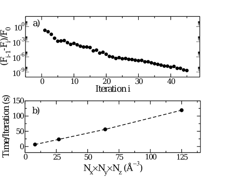Values given above are found to be adequate for all observables presented in this paper. In order to illustrate the high efficiency of the method, the iterative convergence of $F$ with iteration steps is illustrated in figure 2 for the grid described above. After 15 iterations, the convergence in solvation free energy is of the order of $10^{-5}$. We also illustrate in figure 2 the CPU time per iteration for 18 angles per node and $2^{3}$, $3^{3}$, $4^{3}$ and $5^{3}$ nodes per ų for our model system containing several hundred atoms. One observes a linear scaling in $N_{x}\times N_{y}\times N_{z}$, which leads to convergence in less than 15 minutes for the $4\times 4\times 4$ grid per ų described above on an ordinary laptop without parallelization.

Figure 2: a) Variation of the solvation free energy functional $F$ between two iterations normalized by the initial value $F_{0}$ during the iteration process. The grid is composed of $4\times 4\times 4$ nodes per ų and 18 discrete orientations per node. A typical minimization is performed with a precision of $10^{-5}$ in the solvation energy in less than 15 iterations. b) CPU time in seconds per iteration for grid meshes $N_{x}\times N_{y}\times N_{z}=2^{3}$, $3^{3}$, $4^{3}$ and $5^{3}$ per ų and 18 discrete orientations per node. The calculation of the external potential for a given grid mesh is done only once at the beginning of the simulation and takes a CPU time comparable to 1 to 2 iterations. The solvated solute consists of 1280 point charges and 1152 Lennard-Jones sites, for which parameters are extracted from the popular CLAYFF force field Cygan, Liang, and Kalinichev (2004) and given in table 2. The supercell volume is approximately $68$ nm³.

II.2 Molecular Dynamics

Molecular dynamics simulations were generated for the same surface and solvent molecular models in order to compare with the MDFT results. All simulations were done in the canonical NVT ensemble, with a Nose-Hoover thermostat. After a phase of equilibration, all structural quantities were collected and averaged over 5 ns. The local molecular density $n(\mathbf{r})$ of the Stockmayer fluid is calculated as the time averaged density in elementary volumes of $0.1^{3}$ Å³. The densities perpendicularly to the clay layers can be calculated by averaging the above density in the $(x,y)$ planes. The spatial densities of the average dipoles were calculated in the same way. Molecular dynamics simulations were performed with the DLPOLY package Todorov et al. (2006); DL_ .

II.3 System Description

Pyrophyllite is neutral clay. It is monoclinic of space group $2/m$, perfectly cleaved along orientation $\{001\}$. Two views of a pyrophyllite sheet are provided in figure 3. It consists of a stack of 6 atomic layers. The top layer consists of oxygen (O) and silicon (Si) atoms with a lateral hexagonal symmetry. The central layer consists of aluminum (Al) atoms in $2/3$ of the octahedral sites. Between these two layers is a oxygen-hydrogen (O-H) layer, with O atoms at the center of the hexagons formed by the top Al-O sites. The O-H axis is oriented in the direction of the empty octahedral site. The coordinate $z$ of each site along the normal to the clay surface is given in table 1. The simulation box contains two half clay layers of lateral dimensions $L_{x}\times L_{y}=41.44\times 35.88$ Å², which corresponds to 32 clay unit cells of formula Al₄[Si₈O₂₀](OH)₄. The distance between the surfaces is $L_{z}=45.57$ Å, chosen to recover the bulk density of the Stockmayer fluid at the center of the pore, i.e. $n_{0}=0.0289$ molecule per ų. The simulation supercell is thus $\approx 68$ nm${}^{{}^{3}}$ in periodic boundary conditions, and contains 1280 clay atoms (640 per half clay layer). This pore contains 1600 solvent molecules in the reference all-atom simulations.

Figure 3: Microscopic clay structure, side and top views (red, O; white, H; yellow, Si; cyan, Al). In the top view, only layers above the Al atoms are shown to highlight the hexagonal symmetry of the first O-Si layer, the hydroxyl group (-OH) parallel to the sheet, and the Al position in $2/3$ of the octahedral sites.

type		O	Si	O	H	Al	H	O	Si	O
$z$ (Å)		0.00	0.59	2.18	2.27	3.27	4.27	4.36	5.95	6.54

Table 1: Coordinate $z$ along the normal to the surface of each site of the pyrophyllite. The distance $\Delta z$ between two successive layers is also indicated.

We used the CLAYFF force field for both molecular dynamics simulations and MDFT minimization. It is a general purpose force field for simulations involving multicomponent mineral systems and their interfaces with solutions. Related information is tabulated in table 2. The Stockmayer fluid is described by a 3-sites molecule. The neutral central site interacts via Lennard-Jones potentials only. The external sites have opposite charges of $\pm 1.91$ e, both distant of 0.1 Å from the central site. It results in a solvent molecular dipole of 1.84 D (incidentally, approximately that of a water molecule in the gas phase), and, with the chosen Lennard-Jones parameters that match the reduced parameter set of Pollock and Alder Pollock and Alder (1980), in a dielectric constant of roughly 80, comparable to that of bulk water at room conditions MDF . The parameters for the Stockmayer fluid force field can also be found in table 2. Once again, it is not our purpose here to study the more complex solvation by water, which requires extra terms in the functional, but to demonstrate the possibilities of MDFT in the HRF approximation for a generic polar solvent whose functional is of a good quality.

Molecule	Atom	$\epsilon$ (kJ/mol)	$\sigma$ (Å)	$q$ (e)
Pyrophyllite	Al	5.56388e-6	4.27120	1.575
	Si	7.7005e-6	3.30203	2.100
	OG	0.650190	3.16554	$-1.050$
	OH	0.650190	3.16554	$-0.950$
	HG	0.0	0.0	0.425
Stockmayer	central	1.847	3.024	0.0
	side 1	0.0	0.0	1.91
	side 2	0.0	0.0	$-1.91$

Table 2: Force field used to model the pyrophyllite solute and the Stockmayer fluid in both molecular dynamics simulations and HRF-MDFT minimization. Pyrophyllite parameters are extracted from the CLAYFF force field Cygan, Liang, and Kalinichev (2004).

III Results

We first compare the predictions of HRF-MDFT for the solvent density and orientation to reference all-atom simulations, which are two orders of magnitude slower to acquire. We then analyze the role of electrostatic interactions on these quantities.

III.1 Density Profiles

The main structural observable describing solvated interfaces is the number density profile $n(z)$, defined as the average of the number density on plane $z$,

$$n(z)=\frac{1}{L_{x}L_{y}}\iint\frac{n(\mathbf{r})}{n_{0}}dxdy.$$ (16)

The density profiles extracted from explicit molecular dynamics and from HRF-MDFT are given in figure 4. Good overall agreement is found between the two methods. A shoulder followed by two main peaks are found in MD. In HRF-MDFT, the shoulder looks more like a weak peak. The two strongest peaks are followed by long-ranged oscillations. The first feature (shoulder or weak peak) is found at $z=8.3$ Å, 1.76 Å away of the surface layer (see Table 1 to identify layers coordinates). Its intensity is limited to $\approx 0.7$ in MD and $\approx 1$ in HRF-MDFT. The largest and main peak is at $z=9.5$ Å, 2.96 Å after the top surface layer. An intermediately intense and broad peak is also found at $z=12.3$ Å, 5.76 Å away of the surface. These three structures will later be called “prepeak”, “main peak” and “secondary peak”. Further weak oscillations are found up to 15 Å away from the surface. At the center of the supercell, the density is flat at $n=n_{0}$, namely at the bulk density, which means for solvent molecules to be in bulk, homogeneous, conditions.

Figure 4: Normalized number density profile of the solvent between two pyrophyllite layers as calculated by molecular dynamics (open circles) and HRF-MDFT (black line).

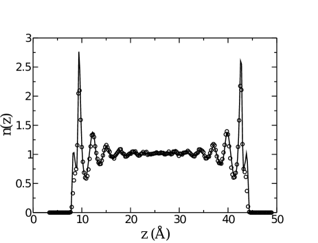
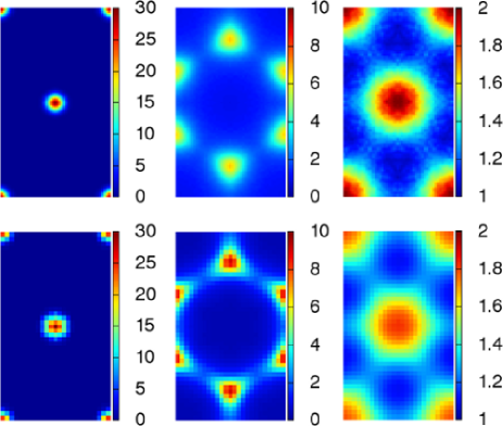
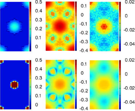
The only noticeable difference lies in the weak prepeak seen in HRF-MDFT observed as a shoulder in molecular dynamics. The HRF-MDFT is known to slightly overestimate the height of the first peak in polarized systems Zhao et al. (2011). The localized nature of the prepeak can be seen in figure 5 where is presented the density map in the plane defined by the maximum of the prepeak, as calculated by MD and HRF-MDFT. The same position and overall shape is found with the two methods. It is slightly broader in-plane in HRF-MDFT for approximately the same intensity, which induces the higher value once averaged in the plane. The prepeak is localized at the center of the hexagons formed by surface Si and O atoms. One may note the high maximum value of the normalized number density $n/n_{0}$ there (up to $\approx 30$). The integral of the density in this peak is the total number of particles in it. While a strict deconvolution of the three-dimensional prepeak is arbitrary, no consistent definition results in more than one solvent molecule inside each prepeak.

In figure 5, we also plot the number density in the plane of the main and secondary peaks. Again, the shapes are very similar in MD and HRF-MDFT. The main peak is localized on top of Si atoms. On the contrary, a depletion is found on top of O atoms of the surface layer. The broad secondary peak can be found again on top of the center of hexagons, i.e. on top of O atoms.

We now have a clear three-dimensional view of the solvent structure on the pyrophyllite surface: rare solvent molecules are adsorbed very close to the surface, at the center of hexagons formed by Si and O atoms of the clay surface layer. On top of these molecules is stacked a strongly structured hexagonal layer of solvent molecules, above Si atoms. An additional, more diffuse layer is found once again on top of the center of the hexagons. The relatively small distance between the first two layers demonstrates significant interactions, and thus cohesion, between layers. This conclusion is in agreement with Rotenberg et al. who showed recently how the competition between adhesion and cohesion determines the hydrophobicity of these surfaces Rotenberg, Patel, and Chandler (2011).
As a partial conclusion about structural properties, HRF-MDFT results are in quantitative agreement with the reference molecular dynamics simulations, with a speed-up of two orders of magnitude.

Figure 5: Maps of the solvent normalized number density $n(\mathbf{r})/n_{0}$ in planes of the prepeak (left), main peak (center) and secondary peak (right), as calculated by molecular dynamics (top) and HRF-MDFT (bottom).

III.2 Orientational Properties

We now turn to the orientational properties of the molecules solvating the pyrophyllite surface. Even if it is routinely done, it is worth emphasizing that orientational properties are slower to sample in molecular dynamics or Monte Carlo simulations as each elementary volume described in section II.2 has to be sampled for a number of angles. This problem is recurrent in numerous simulation techniques where orientational degrees of freedom (from electronic spins to molecular orientations) induces new and rich behaviors Lavrentiev, Nguyen-Manh, and Dudarev (2010); Levesque et al. (2011); Levesque, Gupta, and Gupta (2012). For its part, HRF-MDFT gives a direct access to this quantity through the full orientational density ${\rho\left({\mathbf{r}},{\mathbf{\Omega}}\right)}$, and also the polarization density $\mathbf{P}(\mathbf{r})$ defined in Eq. 13, as one of the two natural observables of the theory.

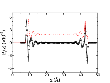
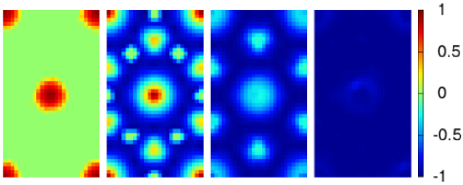
The polarization density is found to be aligned in the $z$ direction, both in MD and HRF-MDFT. In figure 6, we report the projection of $\mathbf{P}$ on the $z$ axis (noted $P_{z}$) as a function of coordinate $z$ (i.e. it is averaged in each plane $z$). Quantitative agreement is again found between the reference molecular dynamics simulations and the HRF-MDFT. A first peak is found at the location of the prepeak, another one at the main peak, etc. Between each maximum, the sign of $P_{z}$ changes. Maps of $P_{z}$ in the planes of the prepeak, main peak and secondary peak are given in figure 7. Similarly to the density, the overall shapes from both methods are in very good agreement. The polarization density is overestimated by HRF-MDFT in the prepeak, which is expected from previous work on small polarized systems Zhao et al. (2011) where the polarization close to the solute is often slightly overestimated. In the main and secondary peaks, the polarization densities are found larger in MD than in HRF-MDFT, although not significantly. This may be due to a balance of the layer-by-layer polarizations in HRF-MDFT.

In order to get more information on the orientational properties per molecule, we also define several orientation order parameters. One is the local orientation of the polarization density, defined as the cosine of the angle between the polarization density $\mathbf{P}(\mathbf{r})$ and the normal $\mathbf{z}$ to the surface,

$$\cos\theta_{P}(\mathbf{r})=\frac{P_{z}\left(\mathbf{r}\right)}{\left\|\mathbf{P}(\mathbf{r})\right\|}.$$ (17)

Another is the averaged molecular orientation

$$\cos\theta_{\mu}(\mathbf{r})=\frac{\left\|P_{z}\left(\mathbf{r}\right)\right\|}{n\left(\mathbf{r}\right)}.$$ (18)

We plot the average molecular orientation $\cos\theta_{\mu}(z)=\left\langle\cos\theta_{\mu}(\mathbf{r})\right\rangle_{xy}$ in figure 8. The solvent molecules show strong average orientation in the first layer. On the contrary, the high polarization density in the second, more cohesive layer reflects the large number of molecules inside, each one with a relatively small preferential orientation along $z$.

Figure 6: Component along the normal $z$ to the surface of the dimensionless solvent polarization density, between two pyrophyllite layers, as calculated by molecular dynamics (open circles) and HRF-MDFT (black line). The density profile is also presented in arbitrary units (red dashed line). Maxima in the polarization density correspond to maxima in the solvent number density.

Figure 7: Maps of the polarization density projected on the normal $z$ to the surface axis, $P_{z}$, in the planes of the prepeak (left), main peak (center) and secondary peak (right), as calculated by molecular dynamics simulations (top) and HRF-MDFT (bottom).

Figure 8: Profile along the normal to the surface $z$ of the average molecular orientation, $\cos\theta_{\mu}(z)$ (black line). The density profile of the solvent is also given in arbitrary units (red dashed line).

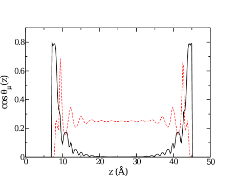
One can get more insight into the orientation properties of the solvent molecules by looking at the order parameter $\cos\theta_{P}$ defined in Eq. 17. When $\cos\theta_{P}=1$ ($-1$), the dipole is oriented against (toward) the surface on the left of the supercell, and vice versa for the other surface. In figure 9, we plot $\cos\theta_{P}$ in the plane of the first three peaks identified earlier and in an intermediate coordinate $z$ between the prepeak and the main peak. We observe that solvent molecules in the prepeak, strongly oriented, point against the surface. In the main peak, dipoles are preferentially oriented toward the surface when localized on top of O atoms. In the secondary layer, preferential polarization is found in the whole plane against the surface.

Figure 9: From left to right, order parameter $\cos\theta_{P}$ in the prepeak, at the intermediate state between the prepeak and the main peak, in the main peak, and in the secondary peak.

III.3 The Role of Electrostatics

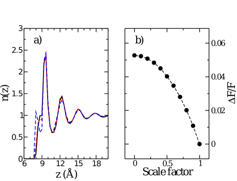
The computational efficiency of the molecular density functional theory unlocks systematic studies of the solvent structure and thermodynamics, such as the relative roles of van der Waals and electrostatic interactions to the CLAYFF force field. They are modeled respectively by Lennard-Jones interactions and a point charge distribution reported in table 2. Figure 10 reports the number density profile along the $z$ axis for modified systems where the CLAYFF charges of the clay atoms have been scaled by a factor of 1, 0.5 and 0. It is observed that, surprisingly, only the shape of the prepeak is modified when the point charges are turned off. This part of the density profile evolves from a localized peak (with electrostatics on) to a shoulder of the main peak when quenched. The rest of the number density profile is unchanged. As might be expected, the polarization vanishes when charges are turned off. In figure 10 is also plotted the relative change in solvation free energy $F\left[\rho\right]$ for scale factors between 0 (turned off) and 1 (completely turned on) of the charges of the clay atoms. The solvation energy is affected by less than 6 % when charges are turned off. The contribution of the electrostatics is thus small compared to the Lennard-Jones one, which is not an obvious result even for a surface with a zero net charge.

Figure 10: a) Number density profile along the $z$ axis with point charges of the clay atoms scaled by a factor of 1 i.e. completely turned on (full black line), 0.5 (dashed red line), and 0 i.e. turned off (blue dashed line). Only the prepeak is affected. b) Relative change in solvation free energy as a function of the scale factor. The relative changes stay below 5.5 %.

IV Conclusion

We have shown that the molecular density functional theory in the homogeneous reference fluid approximation (HRF-MDFT) is able to handle the study of solvation properties of a complex clay surface of several hundred atoms. The description of its structural and orientational properties is quantitatively comparable to reference all-atom molecular dynamics, while reducing the CPU-time by two orders of magnitude. This means that the computation of these properties is now accessible on a simple workstations within minutes. The HRF-MDFT calculations allowed to accurately describe the subtle structure of the first molecular layers at the surface, in particular the orientational properties. The only noticeable difference lies in a localized zone of high density at the center of hexagons, a defect due to a small overestimation of the polarization close to the solute inherent to the method. Some improvements in this respect are in progress.

The numerical efficiency of our approach made it possible to analyze the relative contributions of the CLAYFF force field to the solvation properties. The density profile and the solvation energy are found to be insensitive to the electrostatic contribution. This may imply that the role of electrostatics in charged clays may be reasonably reduced to their charged defects. We think that this finding may be of high interest considering the large amount of work dedicated to the derivation of accurate point charge distributions when building force fields for such systems.

Finally, the next step of this work will be to consider the solvation of clay surfaces by a realistic model of water, at either a dipolar or multipolar level, and by ionic solutions.