^aSchool of Natural Sciences, Institute for Advanced Study, Princeton, NJ 08540, USA

^bDepartment of Particle Physics and Astrophysics, Weizmann Institute of Science,
Rehovot 76100, Israel

^cJadwin Hall, Princeton University, Princeton, NJ 08540, USA

WIS/18/12-NOV-DPPA
 
 
The Thermal Free Energy in Large $N$
Chern-Simons-Matter Theories

Ofer Aharony^a,b, Simone Giombi^c, Guy Gur-Ari^b,
Juan Maldacena^a and Ran Yacoby^b

1 Introduction

An interesting class of conformal field theories in three dimensions comes from coupling a (topological) Chern-Simons (CS) theory to massless matter fields. Since the Chern-Simons coupling is quantized and cannot be renormalized beyond the one-loop level, it is easy to make such theories conformal by tuning away any relevant operators. When the matter fields are purely fermionic this is enough to make the theory conformal. When scalar fields are present there are also classically marginal couplings (of the schematic form $\phi^{6}$ or $\phi^{2}\psi\psi$) and one has to arrange for their beta functions to vanish, but often this can be done, at least in the large $N$ limit.

In the past year, a specific class of conformal Chern-Simons-matter theories has been investigated in detail [1, 2, 3, 4, 5, 6]. This is the large $N$ ’t Hooft limit of a $U(N)$ Chern-Simons theory at level $k$, coupled to a single matter field (scalar or fermion) in the fundamental representation (the generalization to an $O(N)$ theory and/or to $N_{f}$ matter fields is straightforward). The large $N$ limit involves taking both $N$ and $k$ to infinity, keeping fixed the ratio $\lambda\equiv N/k$. These theories come in two versions; a “regular” version where one does not turn on any other couplings except the gauge coupling, and a “critical” version which can be defined by turning on a quartic coupling and sending its coefficient to infinity, or by adding a mass parameter and making it into a dynamical field that is integrated over. It was found that this class of theories has some very nice properties :

• For $\lambda=0$ the theory is free and has an exact high-spin symmetry, with spin $s$ generators for every positive integer $s$. For finite $\lambda$ and large $N$ this symmetry is still approximately present, in the sense that the anomalous dimensions of the high-spin currents are of order $1/N$ [1, 2].

• The approximate high-spin symmetry allows for an exact evaluation of all 2-point and 3-point functions of “single-trace” primary operators, up to two (or three) parameters [7, 8].

• The 2-point and 3-point correlators of these theories can also be computed exactly in the planar limit by resumming Feynman diagrams, and agree with the general results based on symmetries [5, 6].

• It was proposed [1, 2] that these theories (as well as various supersymmetric extensions [3]) have a gravity dual given by a parity breaking version of Vasiliev’s higher-spin theory on $AdS_{4}$ [9, 10], with a parity-breaking parameter $\theta$ that is a function of the ’t Hooft coupling $\lambda$ (the exact gauge theory computation of [5], direct 3-point function calculations in the bulk [11] and arguments in [3] suggest a simple linear relation between the bulk phase $\theta$ and $\lambda$). This duality is a generalization of the original conjectures [12, 13] relating the singlet sector of bosonic/fermionic vector models to the parity invariant Vasiliev’s theories.

• The gravity dual is the same for the theory of scalars coupled to Chern-Simons, and for fermions coupled to Chern-Simons, suggesting a duality between these theories, and this duality is consistent also with their planar $2$-point and $3$-point functions. More precisely, the “critical” version of the scalar theory has the same gravity dual as the “regular” version of the fermionic theory, and vice versa.

In the large $N$ limit, the considerations above suggest an exact duality between the “critical” $U(N)_{k_{\mathrm{YM}}}$ CS theory coupled to a scalar field, and the “regular” $U(k_{\mathrm{YM}})_{-N}$ CS theory coupled to a fermionic field; here we are using the definition of the coupling constant $k_{\mathrm{YM}}$ that arises when the theory is regularized using a Yang-Mills theory at high energies (this is the definition that agrees with the level of the affine Lie algebra that arises on boundaries of the Chern-Simons theory, but many formulas depend on the renormalized coupling $k=k_{\mathrm{YM}}+N\,\mathrm{sign}(k_{\mathrm{YM}})$; in this paper we will generally use this renormalized coupling in all formulas, unless indicated otherwise). In the absence of the matter fields this duality is simply the level-rank duality of pure Chern-Simons theories [14, 15, 16, 17, 18, 19] (and, whenever they are non-zero, the Chern-Simons contributions dominate in the large $N$ limit over those of the matter fields), but the claim is that there is still an exact duality also after adding the matter fields. The duality was conjectured in [5] to hold also for finite values of $N$, with a small shift in the CS level on the fermionic side.

The tests of this (non-supersymmetric) duality so far involve exact computations of various 2-point and 3-point correlation functions in the planar limit, which agree precisely. However, as shown in [8], these correlators are all determined by the almost-conserved high-spin symmetry, and it would be nice to be able to test the duality by properties that are not determined purely by this symmetry. This is particularly important since the gravity dual Vasiliev theory appears to contain additional coupling constants that could affect 5-point and higher correlators of single-trace operators, and their role (if any) in these dualities is still not clear, so one may wonder whether the two theories may have the same 2-point and 3-point functions for their single-trace operators (determined by the high-spin symmetry) but still not be identical.

In this paper we provide further evidence for this duality by matching the thermal free energy between the two theories mentioned above, at large enough temperatures and in the planar limit. The free energy for the fermionic theory was computed already in [1], while the scalar computation (by the same methods) was performed in [4, 20]. These computations do not agree with the duality (nor with supersymmetric versions of the duality, for which there is much more evidence); the scalar computation does not even show a vanishing free energy in the strong coupling limit $\lambda\to 1$ where $\langle T(x)T(y)\rangle$ goes to zero, indicating that it cannot possibly be correct.

The computations in the literature assumed that the eigenvalue distribution of the holonomy of the gauge field around the thermal circle localizes around zero at high enough temperatures, so that the periodicity of the fermionic/scalar fields can be taken to be the naive one (without any shift coming from the gauge holonomy). For free theories this is certainly correct [21, 22]; the matter fields tend to cause the eigenvalue distribution to localize, and while on some spatial manifolds (like $S^{2}$) there is a repulsive term coming from the measure, the effects of this term go to zero at high temperatures. For asymptotically free gauge theories it is also clearly true that the holonomy eigenvalues localize at high enough temperatures. However, for conformal theories at finite coupling it is not clear if this is correct or not.

In section 2 we argue that the correct large $N$ eigenvalue distribution for the thermal gauge holonomy in a Chern-Simons-matter theory of the type described above is not localized, but actually is a uniform distribution with a width covering a fraction $|\lambda|$ of the unit circle. Recall that in our convention $\lambda$ goes from zero at weak coupling to one at strong coupling, so that at weak coupling the eigenvalues do localize as expected, while in the strong coupling limit the eigenvalue distribution becomes uniform (as in a confined phase, though there is no confinement here). This effect comes from the Chern-Simons interactions, that make the eigenvalues effectively fermionic so that they cannot be too dense, despite the attractive forces coming from the matter sector.

In sections 3-5 we compute the thermal free energy for the scalar and fermion theories, both “regular” and “critical”, using this eigenvalue distribution. The computation is completely analogous to the computations of [1, 4, 20], just with a different periodicity condition for the matter fields, arising from the holonomy. We show that with this correct eigenvalue distribution the free energies have the expected properties (going to zero in the strong coupling limit), and that there is a precise matching between the thermal free energies of the scalar and fermion theories. This provides an additional test for the duality between these two theories, that does not follow just from their approximate high-spin symmetry (as far as we know).

In section 6, we then generalize the computation to a theory that has both scalars and fermions, with general couplings. In particular, we verify that in the special case of the theory with $\mathcal{N}=2$ supersymmetry, the thermal free energy in the large $N$ limit is invariant under the supersymmetric version of the duality [23, 24].

Since this paper is rather long, we summarize our results for the free energies of the various theories in section 7. Our analysis of the critical theories automatically gives us the thermal free energies also for the Chern-Simons theories coupled to massive scalars and fermions, and in this section we also briefly discuss some of their properties.

Our methods for computing the holonomy apply to any Chern-Simons-matter theory in which the number of matter fields is much smaller than $N^{2}$ in the large $N$ limit. It would be interesting to understand their implications for theories like those of [25] where the number of matter fields is of order $N^{2}$, so that one cannot neglect their back-reaction on the eigenvalue distribution. This should be important in any computation of the (planar) thermal free energy in these theories. Our methods are sufficient for computing the order $\lambda^{2}$ correction to the free energy in these theories.

It would be interesting to understand how to reproduce our results for the thermal free energy (or various other effects of the Chern-Simons part of the conformal field theory [26, 27]) in the gravity dual theory. It would also be interesting to find additional tests for the field theory duality, in particular for finite values of $N$.

2 The Holonomy Along the Thermal Circle

When one studies the thermodynamics of gauge theories it is common to have long distance modes that require special treatment [28, 29, 30]. These are captured cleanly by thinking of the thermal computation as a Kaluza-Klein reduction of the Euclidean theory on a circle. If we go to energies lower than the inverse radius of the circle (the temperature), we might encounter light degrees of freedom that contribute to the free energy. In particular, the holonomy of the gauge field on the circle is classically a massless field. These light degrees of freedom need to be taken into account correctly.

In our case, we are interested in conformal field theories coming from large $N$ $U(N)$ Chern-Simons theories coupled to matter fields in the fundamental representation. On general grounds, the free energy of a 3d conformal field theory at temperature $T$ and volume $V$ is proportional, for large enough volumes, to $VT^{2}$. For a standard gauge theory coupled to fields in the fundamental representation, the large $N$ free energy would be dominated by the contribution of the gauge fields (scaling as $N^{2}$), while the matter field contributions scale as $N$. In our case, the Chern-Simons theory is purely topological, so the contributions of this theory on its own are independent of the volume, and one thus expects the free energy to scale as $N$. One may expect that at large enough volumes (or, equivalently, large enough temperatures) the contribution of the matter fields will be dominant, and will make the eigenvalues of the holonomy matrix of the gauge field localize near zero (as in asymptotically free gauge theories). This is the assumption that was made in previous computations of the free energy. However, we will see that the presence of the Chern-Simons theory modifies this, even at very large volumes.

In order to analyze the thermal partition function, we reduce the Euclidean theory on the thermal circle of circumference $\beta=1/T$. For the purposes of this section, we begin by integrating out the matter fields in the fundamental representation (at finite temperature and coupling we expect all these fields to be massive). We are then left with an effective two dimensional theory, involving the dimensional reduction of the gauge field. We have the two dimensional gauge fields, and also the holonomy of the gauge field along the thermal circle,

$$a\equiv i\int_{0}^{\beta}dx^{3}A_{3}.$$ (2.1)

The $i$ is introduced so that $a$ is hermitian (we use a convention in which the $A_{\mu}$ fields are anti-Hermitian).

Let us first consider this dimensional reduction for the pure Euclidean Chern-Simons theory,

$$S_{\mathrm{CS}} =\frac{ik}{4\pi}\int\!d^{3}x\,\epsilon^{\mu\nu\rho}\,\mathrm{Tr}\left(A_{\mu}\partial_{\nu}A_{\rho}-\frac{2i}{3}A_{\mu}A_{\nu}A_{\rho}\right)\,,\quad k\in\mathbb{Z}\,.$$ (2.2)

In that case we get an effective action of the form

$$S={k\over 2\pi}\int\!d^{2}x\,\mathrm{Tr}(Fa),$$ (2.3)

where $a$ is the holonomy (which is a scalar field in two dimensions), and $F$ is the field strength along the two non-compact dimensions. Since the original action is topological, this action is also topological.

Let us now compactify one of the $\mathbb{R}^{2}$ directions on a circle of circumference $L$, and think of the other non-compact direction as (Euclidean) time. We now have a second holonomy,

$$b\equiv i\int_{0}^{L}dx^{1}A_{1}.$$ (2.4)

We can gauge fix the other component of the gauge field $A_{0}$ to zero, and the two dimensional action then becomes a quantum mechanics action for the two holonomies, of the form

$$S={ik\over 2\pi}\int\!dt\,\mathrm{Tr}(a\partial_{0}b).$$ (2.5)

This has the form of a matrix quantum mechanics action with a single matrix degree of freedom, since $b$ is canonically conjugate to $a$. We can diagonalize $a$ and consider only the dynamics of the eigenvalues. As is standard in matrix quantum mechanics, this introduces a Vandermonde determinant from the measure, which we can swallow into the wavefunction, but this makes the remaining part of the wavefunction anti-symmetric in the eigenvalues, so they need to be treated as identical (due to the remaining Weyl symmetry) fermions [31]. Thus, we get a Euclidean action for $N$ fermionic variables [32],

$$S={ik\over 2\pi}\sum_{i=1}^{N}\int\!dt\,\dot{b}_{i}a_{i}.$$ (2.6)

For each eigenvalue we have the action for a particle in a magnetic field, on the lowest Landau level. Due to the fact that $a_{i}$ and $b_{i}$ come from holonomies, they all have periodic identifications, which in our normalization are $a_{i}\sim a_{i}+2\pi$ and $b_{i}\sim b_{i}+2\pi$. So we have $N$ fermions moving on a torus, with a magnetic field that has $k$ units of flux. Having flux $k$ implies that each Landau level has precisely $|k|$ states. So, we have $N$ fermions filling $|k|$ states. In our conventions $k$ is the renormalized Chern-Simons coupling (which for the $SU(N)$ part of the gauge group is related to the Chern-Simons coupling that arises from a Yang-Mills regularization by $k=k_{\mathrm{YM}}+N{\mathrm{sign}}(k_{\mathrm{YM}})$), so we always have $|k|>N$, and we have ${|k|\choose N}$ different ways of filling these states. In the pure Chern-Simons theory the Hamiltonian vanishes, so all these states have the same energy (zero energy), giving the ground state degeneracy of the $U(N)$ Chern-Simons theory on a spatial torus [32].

Up to now our analysis was exact. Next, we add the matter in the fundamental representation of the gauge group, in the large $N$ limit. We imagine that the thermal circle is much smaller than the other circle, and we expect all the matter fields to obtain masses of the order of the temperature. When we integrate out the matter fields we get a contribution to the free energy of order $N$ times the volume. In this computation (which we will perform in detail in the subsequent sections for a specific holonomy) we treat the holonomy as a constant background field, so we obtain a result which depends on the holonomy. In the limit where the thermal circle is much smaller than the other circles, the other effects of the gauge field are very small. The most important term that we get in the effective action is then a potential for the holonomy

$$\int dtdx^{1}V(a),$$ (2.7)

where $V(a)$ is some (gauge-invariant) functional of the holonomy, which scales as $N$ in the large $N$ limit. (Additional terms depending on the two dimensional gauge fields also arise when integrating out the matter fields, and we will discuss them below.) At least to leading order in the $1/k$ expansion, the potential $V(a)$ has a minimum at $a=0$, and the expansion around zero looks like $V(a)-V(0)\propto\mathrm{Tr}(a^{2})T^{2}$.

One may be tempted to set $a=0$, as was done in previous computations in thermal Chern-Simons-matter theories. However, recall that when we consider this theory compactified on an extra $S^{1}$, we saw that the eigenvalues of the holonomy $a$ behave like the positions of fermions in the lowest Landau level. Thus, we cannot set them all to zero; the state $a_{i}=0$ is not consistent with the Pauli exclusion principle. The best we can do is to fill a Fermi sea so that the $N$ levels are as close to zero (in the $a$ direction) as possible. Since $ka_{i}/2\pi$ is the conjugate momentum to $b_{i}$, which has periodicity $2\pi$, if we work in a basis of eigenstates of $a_{i}$, then the eigenvalues are quantized in units of $(2\pi/|k|)$. We want to fill the $N$ eigenstates that are closest to $a=0$. In the “phase space” torus parameterized by $a$ and $b$, this means that we are filling all states in a band of width $2\pi|\lambda|$ around $a=0$, and uniform in the $b$ direction, see figure 1(b). Notice that in the large $N$ limit, we have many eigenvalues and we can view the distribution of fermions as a fluid, ignoring the details of the wavefunctions of these fermionic eigenvalues on the torus.

Figure 1: (a) One out of many possible configurations of fermions in the lowest Landau level on the torus. (b) The potential generated by integrating out the matter fields selects the configuration where the fermions are localized in a band around $a=0$. The fact that $L\gg\beta$ breaks the symmetry between the two holonomies.

The matter contributions break the degeneracy between the different ground states of the Chern-Simons theory, and imply that this specific state has the lowest energy. We will argue below that the other contributions from integrating out the matter fields do not affect this computation at leading order in the large $N$ limit. In principle we should now sum over all the different states with a thermal distribution. The energy density difference between the lowest energy state that we found and the next state is of order $T^{3}/|k|$ (since we can shift a single eigenvalue by $2\pi/k$). Thus, if $VT^{2}$ is much larger than $N$ and $k$, we can focus on the ground state, and ignore all other contributions to the free energy. From here on we will be working in this limit for simplicity. The regime $VT^{2}\sim 1$ was discussed in [26, 27].

The discussion above implies that at large volumes/temperatures we should diagonalize the thermal holonomy and distribute the eigenvalues uniformly in a band of width $2\pi|\lambda|$ around zero. It is important that even though to derive this result we compactified an extra circle, this width is independent of the radius of the second spatial circle that we used for this derivation, as long as $L\gg\beta$. So, this distribution of holonomy eigenvalues affects the extensive part of the free energy (the part that is proportional to the radius of the second circle). It turns out that this change in the eigenvalue distribution affects the thermal free energy already at order $\lambda^{2}$ in the weak coupling expansion. As a consistency check on this value for the holonomy, one can check that with this eigenvalue distribution the traces of the holonomy matrix $e^{a}$ transform in the correct way under the level-rank duality (the traces of this holonomy in symmetric representations in the theory with coupling $\lambda$ are mapped to the traces of the holonomy in anti-symmetric representations in the theory with coupling $\lambda-{\mathrm{sign}}(\lambda)$). This would not be the case for $a=0$.

It seems surprising that a finite-volume effect like the eigenvalues being fermions modifies the free energy even in the large volume limit. We can obtain an alternative perspective on this by following the standard treatment of long distance modes in thermal gauge theories [30], adapted for Chern-Simons matter theories. Again, we consider for simplicity the large $k$ limit (with large $N$, and with $\lambda=N/k$ fixed and small). Then, after dimensionally reducing on the circle we get the following effective action

$$S=\int d^{2}x\left[{k\over 2\pi}\mathrm{Tr}(Fa)+T^{2}\mathrm{Tr}(a^{2})+\cdots\right],$$ (2.8)

where we expanded around $a=0$ and kept just the leading terms, ignoring coefficients of order one. We can now integrate out the scalar field $a$, obtaining

$$S\propto{k^{2}\over T^{2}}\int\!d^{2}x\,\mathrm{Tr}(F^{2}).$$ (2.9)

This is a two dimensional Yang-Mills action with an effective coupling $g^{2}_{2D}\propto{T^{2}\over k^{2}}$. So for large $k$ this is very weakly coupled at the scale $T$. In two dimensional Yang-Mills there are no propagating degrees of freedom, but there are non-trivial flux excitations. Here we are interested in the ground state energy of this effective two dimensional Yang-Mills theory. We again compactify the $x^{1}$ direction on a circle of circumference $L$. Choosing the other direction to be time, we end up with a matrix quantum mechanics for the holonomy $b=i\int_{0}^{L}dx^{1}A_{1}$ around the $x^{1}$ direction. Again we have free fermions by diagonalizing the matrix; this time we have free fermions on a circle. The effective Lagrangian takes the form

$$S\propto\int dt{1\over L}{k^{2}\over T^{2}}\sum_{i=1}^{N}\dot{b}_{i}^{2}.$$ (2.10)

Since $b_{i}$ is periodic with period $2\pi$, the quantized momenta for $b_{i}$ have the form $p_{i}=n_{i}$ with integer $n_{i}$, where $p_{i}\sim{k^{2}\over LT^{2}}\dot{b}_{i}$. We fill the Fermi sea up to $|n|=N/2$ and we end up with a ground state energy of the form

$$E_{0}\propto\sum_{n_{i}=-N/2}^{N/2}{LT^{2}\over k^{2}}n_{i}^{2}\propto{LT^{2}N^{3}\over k^{2}}\propto{LT^{2}N\lambda^{2}}.$$ (2.11)

In particular, we see that it is proportional to $L$, so it is an extensive contribution. And, we see that it is (at leading order in perturbation theory) an order $\lambda^{2}$ correction to the leading order in $N$ result for the free energy (that would come from the vacuum energy of the matter fields themselves); thus, it cannot be ignored in the large $N$ limit. As usual, in order to speak in a meaningful way about the ground state energy we need to define a subtraction scheme. The fact that the scheme we used here is the correct one is most transparent according to our previous discussion, where we started from the dimensional reduction of Chern-Simons theory and viewed the same correction to the energy as arising from integrating out the matter fields in the fundamental representation.

As we integrate out matter fields, we also induce terms of the form

$$\int\!d^{2}x\,\mathrm{Tr}\!\left((Da)^{2}\right)+\beta^{2}\mathrm{Tr}\!\left(F^{2}\right),$$ (2.12)

with order one coefficients (depending on $\lambda$) and with powers of the temperature fixed by dimensional analysis. Such terms do not affect the previous discussions, because they are subleading in the $1/N$ expansion.

The spreading of the eigenvalues of the holonomy is expected to be a general feature in the thermodynamics of Chern-Simons-matter theories. For a finite number of matter fields in the fundamental representation we saw that the eigenvalues have a uniform distribution with a width proportional to $|\lambda|$, with corrections that are small at large $N$. It is more complicated to analyze what happens when the number of matter fields is of order $N^{2}$; in that case corrections like (2.12) are no longer negligible, and could affect the eigenvalue distribution. The precise eigenvalue distribution could also depend on the precise field content, since (for instance) for adjoint matter fields the potential $V(a)$ depends only on differences between eigenvalues. In any case, we expect that there should be a non-trivial eigenvalue distibution also in such cases, which would give extra terms starting at order $\lambda^{2}$ in the thermal partition function. In particular, these effects should be added to the results in [35], and to any other perturbative computations of the thermodynamics of Chern-Simons-matter theories.

The derivation we have presented here is most clear if we consider the free energy for the theory on $T^{2}\times S_{\beta}^{1}$. In this case the $T^{2}$ gives us the extra circle that we needed to run our argument, and we can take the large volume limit of the $T^{2}$ and obtain the extensive part of the free energy as we discussed above. One could wonder if similar effects also appear when we consider the three dimensional theory on $\Sigma_{2}\times S_{\beta}^{1}$ for other Riemann surfaces $\Sigma_{2}$, in the limit that $S^{1}_{\beta}$ is very small. Pure three dimensional Chern-Simons theory on such manifolds was studied in detail in [34]. They argued that the theory can be reduced to a two dimensional theory of the form (2.3), where now the integral is over $\Sigma_{2}$. In addition, we can further diagonalize the holonomy in the circle direction. The resulting effective action is independent of the manifold, up to overall factors (involving powers of the Vandermonde determinant) which do not scale like the volume of $\Sigma_{2}$, and thus do not contribute to the free energy in the limit of large $\Sigma_{2}$ volume. Since the analysis on the torus gave us an extensive effect, we expect that the same effect should arise on a general Riemann surface $\Sigma_{2}$. It would be nice to show in detail how this works. A particularly interesting case is when $\Sigma_{2}=S^{2}$. It was argued in [36] (for $\lambda=0$) that the thermal circle needs to be very small, of order $1/\sqrt{N}$ as compared to the size of the $S^{2}$, in order to obtain an answer for the free energy that is linear in $N$. Note that here we are also discussing very large temperatures of the same order. On the sphere, there is a volume independent contribution to the effective action for the thermal holonomy, $a$, that leads to a repulsion between eigenvalues. This will lead to an eigenvalue distribution that is uniformly spread over the whole circle for small temperatures, but for very large temperatures this is overwhelmed by the effects we encountered on the torus. For negatively curved $\Sigma_{2}$ the extra volume independent factors lead to attractive interactions between the eigenvalues, so we expect the eigenvalues to localize already at smaller temperatures.

In the remainder of this paper we will compute the resulting free energy exactly as a function of $\lambda$, but to leading order in the $1/N$ expansion. We work on $\mathbb{R}^{2}$, which can be thought of as the large volume limit of $T^{2}$ (as we mentioned, we expect the result to be the same for large enough volumes on any two dimensional space). The computation is similar to those done in [1, 4, 20]. We simply need to repeat all their steps, but now with a constant holonomy $a$ matrix, with the eigenvalue distribution that we found, in which the eigenvalues of the holonomy are distributed in a band as in figure 1 (b). We view this as a constant background field in the perturbative computation of the free energy.

3 Preliminaries

In the following sections we consider the theory of $N$ complex scalars or Dirac fermions, in the fundamental representation of $U(N)$, coupled to a $U(N)$ gauge field $A_{\mu}$ with Chern-Simons interactions in 3 Euclidean dimensions. The Chern-Simons action (2.2) can be written as

$$S_{\mathrm{CS}} =-\frac{ik}{8\pi}\int\!d^{3}x\,\epsilon^{\mu\nu\rho}\left(A_{\mu}^{a}\partial_{\nu}A_{\rho}^{a}+\frac{1}{3}f^{abc}A_{\mu}^{a}A_{\nu}^{b}A_{\rho}^{c}\right)\,,\quad k\in\mathbb{Z}\,.$$ (3.1)

We take the ’t Hooft large $N$ limit, keeping $\lambda=\frac{N}{k}$ fixed, and work (following [1]) in light-cone gauge in the $x^{1}-x^{2}$ directions, $A_{-}=0$. In this gauge the gluon self-interaction vanishes, and the Chern-Simons action reduces to

$$S_{CS}=\frac{k}{4\pi}\int\!d^{3}x\,A_{+}^{a}\partial_{-}A_{3}^{a}\,.$$ (3.2)

We will regularize our theory by placing a sharp momentum cutoff $\Lambda$ in the $x^{1}-x^{2}$ directions. This will cure most UV divergences, and the remaining ones (that will occur when computing determinants) will be handled as they are encountered. In this regularization (used also in [1, 2, 4, 5]), $k$ is related to the level $k_{\mathrm{YM}}$ that appears in a regularization by a Yang-Mills action (and that appears, for instance, in the Wess-Zumino-Witten model on boundaries) by $k=k_{\mathrm{YM}}+N{\mathrm{sign}}(k_{\mathrm{YM}})$ (for the $SU(N)$ part).

We will take our manifold to be $\mathbb{R}^{2}\times S^{1}$, where the compactified direction is $x^{3}$ and has length $\beta$. As argued in Section 2, we should take the gauge field to have non-trivial holonomy around $S^{1}$ (the eigenvalues of the holonomy are gauge-invariant). We can describe the holonomy in terms of the zero mode

$$\mathcal{A}_{3}=\frac{1}{V_{2}}\int_{\mathbb{R}^{2}}\!d^{2}x\,A_{3}\,,$$ (3.3)

where $V_{2}$ is the regularized volume of $\mathbb{R}^{2}$. Using a residual gauge transformation (that preserves the light-cone gauge) we set $\partial_{3}\mathcal{A}_{3}=0$ and diagonalize $\mathcal{A}_{3}$. In the notations of Section 2, the holonomy along the thermal circle is

$$a\equiv i\beta\mathcal{A}_{3}\,,$$ (3.4)

whose eigenvalues are real and live on a circle of length $2\pi$, due to the periodic identifications which follow from the gauge symmetry.

Most of the calculation can be done for general fixed $a$, but in the end we are interested in the large $N$ limit where the eigenvalues of $a$ are uniformly spread around $0$ with width $2\pi|\lambda|$, namely we take

$$a_{ii}\to a(u)=2\pi|\lambda|u\,,\quad u\in\left[-\frac{1}{2},\frac{1}{2}\right]\,,$$ (3.5)

and replace sums over eigenvalues by integrals over $u$ with uniform distribution over the spread of eigenvalues. In other words, we replace

$$\sum_{i=1}^{N}f(a_{ii})\longrightarrow{N}\int_{-{1\over 2}}^{1\over 2}duf(2\pi|\lambda|u)\,.$$ (3.6)

4 Bosonic Theories

In this section we consider (following [2, 5]) the theory of $N$ complex scalars $\phi$, coupled to the gauge field $A_{\mu}$, defined by the action

$$S =S_{\mathrm{scalar}}+S_{\mathrm{CS}}\,,$$ (4.1)

$$S_{\mathrm{scalar}} =\int\!d^{3}x\,\,(D_{\mu}\phi)^{\dagger}(D^{\mu}\phi)+\frac{\lambda_{6}}{3!N^{2}}(\phi^{\dagger}\phi)^{3}\,,\quad D_{\mu}=\partial_{\mu}+A_{\mu}\,.$$ (4.2)

We include the coupling $\lambda_{6}$ which is exactly marginal in the large $N$ limit [2]. We treat the holonomy as part of the free theory. Its effect is to shift the scalar momentum. Let us define

$$\tilde{p}_{\mu}=p_{\mu}-i\mathcal{A}_{\mu}\,,$$ (4.3)

where $\mathcal{A}_{3}$ is the zero-mode (3.3) and $\mathcal{A}_{\pm}\equiv 0$. We will diagonalize the matrix $\mathcal{A}_{3}$ so that we have $\tilde{p}_{3}=p_{3}-a_{ii}/\beta$ for the $i$’th scalar. The Feynman rules for this theory in momentum space include (in the $A_{-}=0$ gauge)

	$\displaystyle=(\tilde{p}^{-2})_{ji}$
	$\displaystyle=G_{\nu\mu}(p)\delta_{ab}$
	$\displaystyle=i(T^{a}\tilde{p}^{\prime}_{\mu}+\tilde{p}_{\mu}T^{a})_{ij}$
	$\displaystyle=\{T^{a},T^{b}\}_{ij}\delta_{\mu 3}\delta_{\nu 3}$

The non-vanishing components of the gluon propagator are

$$G_{+3}(p)=-G_{3+}(p)=\frac{4\pi i}{k}\frac{1}{p^{+}}\,.$$ (4.4)

It is important that this gluon propagator does not depend on $p_{3}$. Thus, it is not affected by the holonomy.

4.1 Exact propagator

The exact scalar propagator is

$$\langle\phi(p)^{j}\phi^{\dagger}(-q)_{i}\rangle=\left[\frac{1}{\tilde{p}^{2}-\Sigma_{B}}\right]_{\!ji}(2\pi)^{3}\delta^{3}(p-q)\,,$$ (4.5)

where $(\Sigma_{B})_{ji}$ is the sum of 1PI diagrams. As we will see, at large $N$ all contributions to $(\Sigma_{B})_{ji}$ are proportional to the unit matrix in color space, so $\Sigma_{B}(p)_{ji}=\Sigma_{B}(p)\delta_{ji}$. Also, none of the contributions will depend on $p_{3}$. Using this and the fact that $\Sigma_{B}$ must be invariant under rotations in the $x^{1}-x^{2}$ plane, we see that $\Sigma_{B}$ can depend on $p$ only through $p_{s}^{2}=(p_{1})^{2}+(p_{2})^{2}=2p^{+}p^{-}$. Using dimensional analysis, we can write

$$\Sigma_{B}(p)=-\beta^{-2}\mu_{B}^{2}(\lambda,\lambda_{6},\beta p_{s},a)\,,$$ (4.6)

and $\mu_{B}\beta^{-1}=\mu_{B}T$ is the thermal mass of the scalar.

The bootstrap equation for $\Sigma_{B}$ is shown in figure 2. The 1-loop diagram (not shown since it vanishes) can be written as

$$-\int{\mathcal{D}}^{3}q\left[(T^{a}\tilde{q}^{\nu}+\tilde{p}^{\nu}T^{a})\frac{1}{\tilde{q}^{2}-\Sigma_{B}(q)}(T^{a}\tilde{p}^{\mu}+\tilde{q}^{\mu}T^{a})\right]_{ji}G_{\mu\nu}(q-p)\,.$$ (4.7)

It is understood here and below that the full integration measure on $\mathbb{R}^{2}\times S^{1}$ is

$$\int{\mathcal{D}}^{3}q=\frac{1}{\beta}\int_{\mathbb{R}^{2}}\frac{d^{2}q}{(2\pi)^{2}}\sum_{n=-\infty}^{\infty}\,,$$ (4.8)

where momenta $q$ on $S^{1}$ are quantized as $q_{n}=\frac{2\pi n}{\beta}$. It is easy to check that the diagram (4.7) vanishes using the relation for generators in the fundamental representation of $U(N)$,

$$T^{a}_{ij}T^{a}_{kl}=-\frac{1}{2}\delta_{il}\delta_{jk}\,,$$ (4.9)

and the fact that $\Sigma_{B}$ and $\tilde{p}$ are diagonal in color space for any vector $p$.

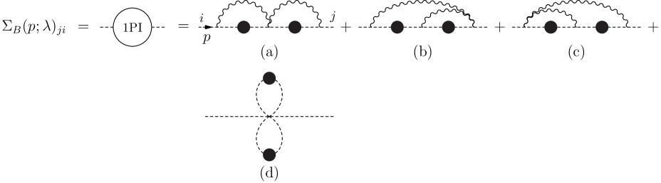
Figure 2: Bootstrap equation for the scalar self-energy. A filled circle denotes the full scalar propagator. (d) corresponds to the insertion of the $\lambda_{6}(\phi^{2})^{3}$ interaction vertex.

In the remaining diagrams, the $\phi\partial_{\mu}\phi^{\dagger}A_{\mu}$ vertex always appears with $\mu\neq 3$, and therefore the Feynman rule for the vertex becomes simply $iT^{a}_{ij}(p+p^{\prime})_{\mu}$. The remaining diagrams can be written as

$$\mathrm{(a)} =-\left(\frac{4\pi}{k}\right)^{2}\int{\mathcal{D}}^{3}l{\mathcal{D}}^{3}q\frac{(l+p)^{+}}{(l-p)^{+}}\frac{(q+p)^{+}}{(q-p)^{+}}\left[T^{b}\frac{1}{\tilde{l}^{2}-\Sigma_{B}(l)}\{T^{a},T^{b}\}\frac{1}{\tilde{q}^{2}-\Sigma_{B}(q)}T^{a}\right]_{ji}\,,$$

$$\mathrm{(b)}=\mathrm{(c)} =\left(\frac{4\pi}{k}\right)^{2}\int{\mathcal{D}}^{3}l{\mathcal{D}}^{3}q\frac{(l+p)^{+}}{(l-p)^{+}}\frac{(q+l)^{+}}{(q-l)^{+}}\left[T^{a}\frac{1}{\tilde{l}^{2}-\Sigma_{B}(l)}T^{b}\frac{1}{\tilde{q}^{2}-\Sigma_{B}(q)}\{T^{a},T^{b}\}\right]_{ji}\,,$$

$$\mathrm{(d)} =-\frac{1}{2}\frac{\lambda_{6}}{N^{2}}\int{\mathcal{D}}^{3}l{\mathcal{D}}^{3}q\left[\frac{1}{\tilde{q}^{2}-\Sigma_{B}(q)}\right]_{j_{1}i_{1}}\left[\frac{1}{\tilde{l}^{2}-\Sigma_{B}(l)}\right]_{j_{2}i_{2}}\times$$

$$\quad\qquad\qquad\;\;\left[\delta_{ij}\delta_{i_{1}j_{1}}\delta_{i_{2}j_{2}}+(5~{}\mathrm{permutations})\right]\,.$$ (4.10)

In diagram (d) the one-half is a symmetry factor. For general matrices $A,B$ we have, using (4.9),

$$T^{b}A\{T^{a},T^{b}\}BT^{a}=T^{b}AT^{a}B\{T^{a},T^{b}\}=\frac{1}{4}[BA+\mathrm{Tr}(A)\mathrm{Tr}(B)\mathbb{1}]\,.$$ (4.11)

Using this in diagrams (a)-(c), we see that the first term of (4.11) is subleading at large $N$ and can be dropped. In diagram (d), only the first permutation survives at large $N$. The diagrams can therefore be written as

$$\mathrm{(a)} =-\frac{4\pi^{2}}{k^{2}}\delta_{ji}\left[\int{\mathcal{D}}^{3}q\frac{(q+p)^{+}}{(q-p)^{+}}\mathrm{Tr}\left(\frac{1}{\tilde{q}^{2}-\Sigma_{B}(q)}\right)\right]^{2}\,,$$ (4.12)

$$\mathrm{(b)}=\mathrm{(c)} =\frac{4\pi^{2}}{k^{2}}\delta_{ji}\int{\mathcal{D}}^{3}l{\mathcal{D}}^{3}q\frac{(l+p)^{+}}{(l-p)^{+}}\frac{(q+l)^{+}}{(q-l)^{+}}\mathrm{Tr}\left(\frac{1}{\tilde{q}^{2}-\Sigma_{B}(q)}\right)\mathrm{Tr}\left(\frac{1}{\tilde{l}^{2}-\Sigma_{B}(l)}\right)\,,$$

$$\mathrm{(d)} =-\frac{\lambda_{6}}{2}\delta_{ji}\left[\frac{1}{N}\int{\mathcal{D}}^{3}q\mathrm{Tr}\left(\frac{1}{\tilde{q}^{2}-\Sigma_{B}(q)}\right)\right]^{2}\,.$$

We can simplify things by taking the derivative of the bootstrap equation

$$\Sigma_{B}(p)\delta_{ij}=\mathrm{(a)}+\mathrm{(b)}+\mathrm{(c)}+\mathrm{(d)}$$ (4.13)

with respect to $p^{-}$, using the relations

$$\frac{\partial}{\partial p^{-}}\frac{1}{p^{+}}=2\pi\delta^{2}(p)\,,\quad\frac{\partial p_{s}}{\partial p^{-}}=\frac{p^{+}}{p_{s}}\,.$$ (4.14)

The resulting equation is $\partial_{p^{-}}\Sigma_{B}(p)=0$, and therefore $\Sigma_{B}$ and $\mu_{B}^{2}$ do not depend on $p_{s}$. Using this observation, we can simply evaluate the various contributions to $\Sigma_{B}$ by setting $p_{s}=0$. With this choice, one finds that (b)=(c)=0 for symmetry reasons, and

$$\mathrm{(a)} =-4\pi^{2}\lambda^{2}\delta_{ji}\left[\int^{1/2}_{-1/2}du\int{\mathcal{D}}^{3}q\frac{1}{\tilde{q}^{2}+\beta^{-2}\mu_{B}^{2}}\right]^{2}\,,$$ (4.15)

$$\mathrm{(d)} =-\frac{\lambda_{6}}{2}\delta_{ji}\left[\int^{1/2}_{-1/2}du\int{\mathcal{D}}^{3}q\frac{1}{\tilde{q}^{2}+\beta^{-2}\mu_{B}^{2}}\right]^{2}\,,$$ (4.16)

where we have replaced the trace with an integral over the uniform spread of eigenvalues. The sum over the $q_{3}$ momentum takes the form

$$F(q_{s},u) \equiv\frac{1}{\beta}\sum_{n=-\infty}^{\infty}\frac{1}{(\frac{2\pi}{\beta}(n+|\lambda|u))^{2}+q_{s}^{2}+\beta^{-2}\mu_{B}^{2}}$$

$$=\frac{\beta}{2\sqrt{(\beta q_{s})^{2}+\mu_{B}^{2}}}\cdot{\mathrm{Re}}\left(\coth\left[\frac{\sqrt{(\beta q_{s})^{2}+\mu_{B}^{2}}+2\pi i|\lambda|u}{2}\right]\right)\,\,.$$ (4.17)

The bootstrap equation for the self-energy can then be written as

$$\Sigma_{B}=-\hat{\lambda}^{2}\left[\int^{1/2}_{-1/2}du\int dq_{s}q_{s}F(q_{s},u)\right]^{2}\,,$$ (4.18)

where we defined

$$\hat{\lambda}^{2}\equiv\lambda^{2}+\frac{\lambda_{6}}{8\pi^{2}}\,.$$ (4.19)

The thermal mass $\mu_{B}$ then obeys the bootstrap equation

$$|\mu_{B}(\lambda,\lambda_{6})|=\left|\frac{\hat{\lambda}}{2}\int^{1/2}_{-1/2}du\int_{0}^{\infty}dx\frac{x}{\sqrt{x^{2}+\mu_{B}^{2}}}\,{\mathrm{Re}}\left(\coth\left[\frac{\sqrt{x^{2}+\mu_{B}^{2}}+2\pi i|\lambda|u}{2}\right]\right)\right|\,.$$ (4.20)

In writing this we made a change of variables $x=\beta q_{s}$, and took the square root of the equation for $\Sigma_{B}$. Using a cutoff $\Lambda^{\prime}=\beta\Lambda$, we find that the radial integral gives (using ${\mathrm{Re}}(\log(z))=\log|z|$)

$$2\log\left|\sinh\left(\frac{\sqrt{x^{2}+\mu_{B}^{2}}+2\pi i|\lambda|u}{2}\right)\right|_{x=0}^{\Lambda^{\prime}}=\Lambda^{\prime}-2\log\left|2\sinh\left(\frac{|\mu_{B}|+2\pi i|\lambda|u}{2}\right)\right|+O\left(\frac{1}{\Lambda^{\prime}}\right)\,.$$ (4.21)

Subtracting the divergence using a mass counter-term, and taking the limit $\Lambda\to\infty$, the bootstrap equation for $\mu_{B}$ now reads

$$|\mu_{B}| =\left|\hat{\lambda}\int^{1/2}_{-1/2}du\log\left|2\sinh\left(\frac{|\mu_{B}|+2\pi i|\lambda|u}{2}\right)\right|\right|\,.$$ (4.22)

This integral can be computed analytically in terms of dilogarithms, and we find the equation

$$\pm\mu_{B} =-\frac{|\hat{\lambda}\mu_{B}|}{2}-\frac{1}{2\pi i}\frac{|\hat{\lambda}|}{|\lambda|}\left[\mathrm{Li}_{2}(e^{-|\mu_{B}|-\pi i|\lambda|})-\mathrm{Li}_{2}(e^{-|\mu_{B}|+\pi i|\lambda|})\right]\,.$$ (4.23)

In some cases there may be more than one solution to this equation (with different choices of the relative sign), and in such cases we should choose the solution that minimizes the free energy. We can always take (without loss of generality) $\mu_{B}>0$, and we will do this in the rest of this section. The solution that minimizes the free energy is then always the one with the plus sign in (4.23).

To summarize, the exact scalar propagator is given by

$$\langle\phi(p)^{j}\phi^{\dagger}(-q)_{i}\rangle=\left[\frac{1}{\tilde{p}^{2}+\beta^{-2}\mu_{B}^{2}(\lambda,\lambda_{6})}\right]_{\!ji}(2\pi)^{3}\delta^{3}(p-q)\,,$$ (4.24)

where the thermal mass $\mu_{B}$ is found by solving (4.23). Note that if we drop the integral over the holonomy in (4.22) and set $u=0$, the equation determining the thermal mass agrees with the result derived in [4, 20].

4.2 Free energy

It was shown in [4, 20] that the free energy has a simple expression in terms of the self-energy. In our case the calculation follows through, except that we should include the integral over the holonomy. At large $N$, we have

$$\beta F_{B}=NV_{2}\int_{-1/2}^{1/2}du\int\frac{d^{2}p}{(2\pi)^{2}}\sum_{n=-\infty}^{\infty}\left[\log\left(\tilde{p}^{2}-\Sigma_{B}\right)+\frac{2}{3}\frac{\Sigma_{B}}{\tilde{p}^{2}-\Sigma_{B}}\right]\,,$$ (4.25)

where $p_{3}=\frac{2\pi n}{\beta}$ and $\tilde{p}_{\mu}=p_{\mu}-{2\pi|\lambda|u\over\beta}\delta_{3,\mu}$.

Consider first the log term. The sum over $n$ diverges, and we regulate it by introducing a negative contribution with a large mass $\beta^{-1}M$, so that we need to compute (here we use that $\Sigma_{B}=-\beta^{-2}\mu_{B}^{2}$)

$$\int\frac{d^{2}p}{(2\pi)^{2}} \sum_{n=-\infty}^{\infty}\log\left[\frac{\tilde{p}^{2}+\beta^{-2}\mu_{B}^{2}}{\tilde{p}^{2}+\beta^{-2}M^{2}}\right]=\int\frac{d^{2}p}{(2\pi)^{2}}\log\prod_{n=-\infty}^{\infty}\left[1+\frac{p_{s}^{2}+\beta^{-2}\mu_{B}^{2}}{\left(\frac{2\pi}{\beta}(n-|\lambda|u)\right)^{2}}\right]-(\mu_{B}\to M)$$

$$=\int\frac{d^{2}p}{(2\pi)^{2}}\log\left[\cosh(\beta\sqrt{p_{s}^{2}+\beta^{-2}\mu_{B}^{2}})-\cos(2\pi|\lambda|u)\right]-(\mu_{B}\to M)$$

$$=\frac{1}{2\pi\beta^{2}}\int_{0}^{\Lambda^{\prime}}\!dx\,x\log\left[2\cosh(\sqrt{x^{2}+\mu_{B}^{2}})-2\cos(2\pi|\lambda|u)\right]-(\mu_{B}\to M)\,,$$ (4.26)

where again $x=\beta p_{s}$ and $\Lambda^{\prime}=\beta\Lambda$. The first term has a UV power divergence, which we now subtract. We can write this term as

$$\frac{1}{2\pi\beta^{2}}\int_{0}^{\Lambda^{\prime}}\!dx\,x\left\{\sqrt{x^{2}+\mu_{B}^{2}}+\log\left[1+e^{-2\sqrt{x^{2}+\mu_{B}^{2}}}-2e^{-\sqrt{x^{2}+\mu_{B}^{2}}}\cos(2\pi|\lambda|u)\right]\right\}\,.$$ (4.27)

The divergence is now contained in the first term. The last term, which is finite, can be simplified by taking $y=\sqrt{x^{2}+\mu_{B}^{2}}$ and sending $\Lambda\to\infty$. After subtracting the divergence we find

$$\frac{1}{2\pi\beta^{2}}\left[-\frac{\mu_{B}^{3}}{3}+\int_{\mu_{B}}^{\infty}\!dy\,y\log\left(1+e^{-2y}-2e^{-y}\cos(2\pi|\lambda|u)\right)\right]\,.$$ (4.28)

Let us now compute the integral $\int_{-1/2}^{1/2}du$ of this expression. With some work, one finds the result

$$\frac{1}{2\pi\beta^{2}}\left\{-\frac{\mu_{B}^{3}}{3}-\frac{1}{\pi i|\lambda|}\int_{\mu_{B}}^{\infty}\!dy\,y\left[\mathrm{Li}_{2}(e^{-y+\pi i|\lambda|})-\mathrm{Li}_{2}(e^{-y-\pi i|\lambda|})\right]\right\}\,.$$ (4.30)

This is the first term in (4.26). The second, regulator term in (4.26) gives a pure UV divergence (when taking $M,\Lambda\to\infty$) that we subtract. This removes the determinant regulator.

Let us now consider the second term in (4.25). Here the computation is similar to what we encountered in section 4.1. The bootstrap equation for the self-energy implies that

$$\mu_{B}=\pm 2\pi|\hat{\lambda}|\int_{-1/2}^{1/2}du\int\frac{d^{2}p}{(2\pi)^{2}}\sum_{n=-\infty}^{\infty}\frac{1}{\tilde{p}^{2}+\beta^{-2}\mu_{B}^{2}}\,,$$ (4.31)

and so we find that

$$\frac{2}{3}\int_{-1/2}^{1/2}du\int\frac{d^{2}p}{(2\pi)^{2}}\sum_{n=-\infty}^{\infty}\frac{\Sigma_{B}}{\tilde{p}^{2}-\Sigma_{B}}=\mp\frac{\mu_{B}^{3}}{3\pi\beta^{2}|\hat{\lambda}|}\,.$$ (4.32)

Combining (4.30) and (4.32), we find that the free energy is given by

$$\beta F_{B}=-\frac{NV_{2}}{2\pi\beta^{2}}\left\{\frac{\mu_{B}^{3}}{3}\left(1\pm\frac{2}{|\hat{\lambda}|}\right)+\frac{1}{\pi i|\lambda|}\int_{\mu_{B}}^{\infty}\!dy\,y\left[\mathrm{Li}_{2}(e^{-y+\pi i|\lambda|})-\mathrm{Li}_{2}(e^{-y-\pi i|\lambda|})\right]\right\}\,,$$ (4.33)

where the choice of sign is correlated to the choice of sign in (4.23). Note that (4.23) is always given by setting to zero the $\mu_{B}$-derivative of (4.33). Using (4.23) we can rewrite (4.33) as

$$\beta F_{B}=-\frac{N}{\lambda}\frac{V_{2}}{2\pi^{2}i\beta^{2}} \left\{\frac{\mu_{B}^{2}}{3}\left[\mathrm{Li}_{2}(e^{-\mu_{B}+\pi i\lambda})-\mathrm{Li}_{2}(e^{-\mu_{B}-\pi i\lambda})\right]\right.$$

$$\quad\left.+\int_{\mu_{B}}^{\infty}\!dy\,y\left[\mathrm{Li}_{2}(e^{-y+\pi i\lambda})-\mathrm{Li}_{2}(e^{-y-\pi i\lambda})\right]\right\}\,.$$ (4.34)

It is obvious from this expression that the free energy vanishes (for fixed $N$) in the strong coupling limit $|\lambda|\to 1$. The free energy with $\lambda_{6}=0$ is shown in figure 4 below.

4.3 The critical theory

In this subsection we consider the critical bosonic theory, which at large $N$ can be defined as the Legendre transform of the regular theory (with $\lambda_{6}=0$) with respect to the scalar operator $\phi^{\dagger}\phi$. In order to carry out the transform, we begin by computing the free energy in the theory deformed by a mass squared $\sigma$, and then we make $\sigma$ into a dynamical field. The mass-deformed theory has the action (4.1), deformed by

$$\delta S=\int\!d^{3}x\,\sigma\phi^{\dagger}\phi\,.$$ (4.35)

The exact propagator (4.5) is now

$$\langle\phi(p)^{j}\phi^{\dagger}(-q)_{i}\rangle=\frac{1}{\tilde{p}^{2}+\sigma-\Sigma_{B}}\delta_{ji}(2\pi)^{3}\delta^{3}(p-q)=\frac{1}{\tilde{p}^{2}-\Sigma_{B,\sigma}}\delta_{ji}(2\pi)^{3}\delta^{3}(p-q)\,.$$ (4.36)

The computation of the bootstrap equation for the self-energy in section 4.1 generalizes to this case with minor modifications. The right-hand side of equation (4.18), given by the sum of 1PI diagrams, is given by the old one with the replacement $\Sigma_{B}\to\Sigma_{B,\sigma}$. If we replace the definition (4.6) with $\Sigma_{B,\sigma}=-\beta^{-2}\mu_{B}^{2}$, the right-hand side is unchanged. In the left-hand side of (4.18) we now have $\Sigma_{B}=\Sigma_{B,\sigma}+\sigma=-\beta^{-2}(\mu_{B}^{2}-\tilde{\sigma})$, where $\tilde{\sigma}\equiv\beta^{2}\sigma$. As a result, the final bootstrap equation (4.23) becomes

$$\pm\sqrt{\mu_{B}^{2}-\tilde{\sigma}}=-\frac{|\lambda|\mu_{B}}{2}-\frac{1}{2\pi i}\left[\mathrm{Li}_{2}(e^{-\mu_{B}-\pi i|\lambda|})-\mathrm{Li}_{2}(e^{-\mu_{B}+\pi i|\lambda|})\right]\,.$$ (4.37)

The free energy written in terms of the self-energy is also slightly modified, and becomes

$$\beta F_{B,\sigma}=NV_{2}\int_{-1/2}^{1/2}du\int\frac{d^{2}p}{(2\pi)^{2}}\sum_{n=-\infty}^{\infty}\left[\log\left(\tilde{p}^{2}-\Sigma_{B,\sigma}\right)+\frac{2}{3}\frac{\Sigma_{B,\sigma}+\sigma}{\tilde{p}^{2}-\Sigma_{B,\sigma}}\right]\,.$$ (4.38)

The extra contribution in the last term can be easily computed analogously to (4.32). The final result for the free energy is given by

$$\beta F_{B,\sigma}=-\frac{NV_{2}T^{2}}{2\pi}\left\{\frac{\mu_{B}^{3}}{3}\pm\frac{2(\mu_{B}^{2}-\tilde{\sigma})^{3/2}}{3|\lambda|}+\frac{1}{\pi i|\lambda|}\int_{\mu_{B}}^{\infty}\!dy\,y\left[\mathrm{Li}_{2}(e^{-y+\pi i|\lambda|})-\mathrm{Li}_{2}(e^{-y-\pi i|\lambda|})\right]\right\}\,.$$ (4.39)

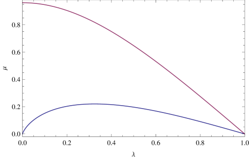
Figure 3: Thermal mass in the regular bosonic theory with $\lambda_{6}=0$ (blue, lower curve) and critical theory (red, upper curve), with arbitrary normalization.

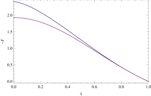
Figure 4: Negative free energy in the regular bosonic theory with $\lambda_{6}=0$ (blue, upper curve) and critical theory (red, lower curve), using arbitrary normalization.

Let us now carry out the path integral over $\sigma$ to obtain the critical theory. The saddle point equation for $\tilde{\sigma}$, derived from (4.39) (using (4.37)), is

$$\sqrt{\mu_{B}^{2}-\tilde{\sigma}}=0\,,$$ (4.40)

and we find $\tilde{\sigma}=\mu_{B}^{2}$. Plugging this back in, we find the free energy of the critical bosonic theory,

$$\beta F_{B}^{\mathrm{crit.}}=-\frac{NV_{2}T^{2}}{2\pi}\left\{\frac{\mu_{B,c}^{3}}{3}+\frac{1}{\pi i\lambda}\int_{\mu_{B,c}}^{\infty}\!dy\,y\left[\mathrm{Li}_{2}(e^{-y+\pi i\lambda})-\mathrm{Li}_{2}(e^{-y-\pi i\lambda})\right]\right\}\,,$$ (4.41)

where $\mu_{B,c}$ is given by (4.37)

$$0=\lambda\mu_{B,c}+\frac{1}{\pi i}\left[\mathrm{Li}_{2}(e^{-\mu_{B,c}-\pi i\lambda})-\mathrm{Li}_{2}(e^{-\mu_{B,c}+\pi i\lambda})\right]\,.$$ (4.42)

These results are shown in figures 3 and 4. It is amusing to note that (4.42) is simply given by setting the $\mu_{B,c}$ derivative of (4.41) to zero.

One may check that in the limit $\lambda=0$ these results agree with the thermal mass and free energy of the critical $O(N)$ model computed in [37]. At $\lambda=0$, one finds from (4.42)-(4.41)

$$\mu_{B,c}=2\log\left(\frac{\sqrt{5}+1}{2}\right)\,,$$ (4.43)

$$\beta F_{B,c}=-NV_{2}T^{2}\,\frac{4}{5}\frac{\zeta(3)}{\pi}\,,$$ (4.44)

which is indeed the result of [37] (up to a factor of 2 in the free energy, due to the fact that we work with $U(N)$ rather than $O(N)$).

5 Fermionic Theories

In this section we consider, following [1], the theory of $N$ Dirac fermions $\psi^{i}$, coupled to the $U(N)$ Chern-Simons gauge field $A_{\mu}$. The theory is defined by the action

$$S =S_{\mathrm{fermion}}+S_{\mathrm{CS}},$$ (5.1)

$$S_{\mathrm{fermion}} =\int\!d^{3}x\,\bar{\psi}\gamma^{\mu}D_{\mu}\psi+\sigma\bar{\psi}\psi\,.$$ (5.2)

The regular theory is given by setting $\sigma=0$. In the critical theory (the Gross-Neveu model with Chern-Simons interactions) $\sigma$ plays the role of the primary scalar operator, and we must perform the path integral over it.

The calculation is similar to the one done in [1]. Our conventions for the gamma matrices are $\gamma^{\mu}=\sigma^{\mu}$, $\mu=1,2,3$, where $\sigma^{\mu}$ are the Pauli matrices. In the thermal theory the fermions have anti-periodic boundary conditions on the thermal $S^{1}$ (before including the effects of the holonomy), so the momenta in this direction are quantized as $p_{3}=\frac{2\pi}{\beta}(n+\frac{1}{2})$, $n\in\mathbb{Z}$.

5.1 Exact propagator

Denote the exact propagator as

$$\langle\psi(p)_{i}\bar{\psi}(-q)_{j}\rangle=\left[\frac{1}{i\tilde{p}_{\mu}\gamma^{\mu}+\sigma-\Sigma_{F}(p)}\right]_{ji}(2\pi)^{3}\delta^{3}(p-q)\,.$$ (5.3)

The notation is the same as for the bosonic theories, with $\Sigma_{F}$ being the sum of 1PI diagrams. The bootstrap equation for $\Sigma_{F}$ is shown in figure 5.

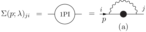
Figure 5: Bootstrap equation for $\Sigma_{F}$. A filled circle denotes the exact fermion propagator.

The $2\times 2$ matrix $\Sigma_{F}$ can be uniquely expanded as the linear combination

$$\Sigma_{F} =i\Sigma_{\mu}\gamma^{\mu}+\Sigma_{I}I=i\Sigma_{-}\gamma^{-}+i\Sigma_{+}\gamma^{+}+i\Sigma_{3}\gamma^{3}+\Sigma_{I}I\,.$$ (5.4)

Let us also define $\tilde{\Sigma}_{I}=\Sigma_{I}-\sigma$. The diagram in the bootstrap equation is given by

$$\mathrm{(a)} =\frac{4\pi i}{k}T^{a}_{jm}T^{a}_{ki}\int\!{\mathcal{D}}^{3}q\,\frac{1}{(q-p)^{+}}\,\gamma^{[3|}\left(\frac{1}{i\tilde{q}_{\mu}\gamma^{\mu}+\sigma-\Sigma_{F}(q)}\right)_{mk}\gamma^{|+]}$$

$$=-\frac{2\pi i}{k}\delta_{ji}\mathrm{Tr}_{N}\int\!{\mathcal{D}}^{3}q\,\frac{1}{(q-p)^{+}}\,\gamma^{[3|}\frac{1}{i\tilde{q}_{\mu}\gamma^{\mu}+\sigma-\Sigma_{F}(q)}\gamma^{|+]}$$

$$=\frac{2\pi i}{k}\delta_{ji}\mathrm{Tr}_{N}\int\!{\mathcal{D}}^{3}q\,\frac{1}{(q-p)^{+}}\frac{1}{(\tilde{q}-\Sigma_{F})^{2}+\tilde{\Sigma}_{I}^{2}}\,\gamma^{[3|}\!\left[i(\tilde{q}-\Sigma_{F})_{\mu}\gamma^{\mu}+\tilde{\Sigma}_{I}I\right]\!\gamma^{|+]}\,,$$ (5.5)

where in the second line we used (4.9). The right-hand side is proportional to the unit matrix in color space, so we may write $\Sigma_{F}(p)_{ji}=\Sigma_{F}(p)\delta_{ji}$. Using the relations $\gamma^{[3|}\gamma^{\mu}\gamma^{|+]}=-2\delta^{\mu}_{-}I$ and $[\gamma^{3},\gamma^{+}]=2\gamma^{+}$, the bootstrap equation becomes

$$\Sigma_{F}(p) =\frac{4\pi i}{k}\mathrm{Tr}_{N}\int\!{\mathcal{D}}^{3}q\,\frac{1}{(q-p)^{+}}\frac{\tilde{\Sigma}_{I}(q)\gamma^{+}-i(q-\Sigma_{F})^{+}I}{(\tilde{q}-\Sigma_{F})^{2}+\tilde{\Sigma}_{I}^{2}}$$

$$=4\pi i\lambda\int_{-1/2}^{1/2}\!du\,\int\!\frac{d^{2}q}{(2\pi)^{2}}\,\frac{1}{(q-p)^{+}}\frac{1}{\beta}\sum_{n=-\infty}^{\infty}\frac{\tilde{\Sigma}_{I}(q)\gamma^{+}-i(q-\Sigma_{F})^{+}I}{(\tilde{q}-\Sigma_{F})^{2}+\tilde{\Sigma}_{I}^{2}}\,.$$ (5.6)

We see that $\Sigma_{-}=\Sigma_{3}=0$, and that $\Sigma_{F}$ is independent of $p^{3}$. Using also rotation invariance in the $p^{1}-p^{2}$ plane, we may therefore write

$$\tilde{\Sigma}_{I}(p)=f(\lambda,\beta p_{s},\tilde{\sigma})p_{s}\,,\quad\Sigma_{+}(p)=g(\lambda,\beta p_{s},\tilde{\sigma})p_{+}\,,$$ (5.7)

where $\tilde{\sigma}\equiv\beta\sigma$. Let us now compute the sum in (5.6). As before, let $x=\beta q_{s}$.

$$\frac{1}{\beta}\sum_{n=-\infty}^{\infty} \frac{1}{(\tilde{q}-\Sigma_{F})^{2}+\tilde{\Sigma}_{I}^{2}(q)}=\frac{1}{\beta}\sum_{n}\frac{1}{\tilde{q}_{3}^{2}+(q-\Sigma_{F})_{s}^{2}+\tilde{\Sigma}_{I}^{2}}$$

$$=\beta\sum_{n}\frac{1}{\left[2\pi\left(n+\frac{1}{2}-|\lambda|u\right)\right]^{2}+x^{2}(1-g+f^{2})}$$

$$=\frac{\beta}{2}\frac{1}{x\sqrt{1-g(x)+f^{2}(x)}}\,{\mathrm{Re}}\left[\tanh\left(\frac{x\sqrt{1-g(x)+f^{2}(x)}+2\pi i|\lambda|u}{2}\right)\right]$$

$$\equiv\frac{\beta}{2}G(x)\,.$$ (5.8)

The bootstrap equation is now (comparing separately the coefficients of $\gamma^{+}$ and $I$)

$$\Sigma_{+}(p) =2\pi\lambda\beta\int_{-1/2}^{1/2}du\,\int\!\frac{d^{2}q}{(2\pi)^{2}}\,\frac{\tilde{\Sigma}_{I}(q)}{(q-p)^{+}}\cdot G(x)\,,$$ (5.9)

$$\Sigma_{I}(p) =2\pi\lambda\beta\int_{-1/2}^{1/2}du\,\int\!\frac{d^{2}q}{(2\pi)^{2}}\,\frac{q^{+}}{(q-p)^{+}}\cdot G(x)\,.$$ (5.10)

Let us differentiate with respect to $p^{-}$, using (4.14). We find

$$\frac{y}{2}\partial_{y}g+g(y) =-yfG(y)\,,$$ (5.11)

$$\partial_{y}f+\frac{f(y)}{y} =-G(y)\,.$$ (5.12)

Combining these, we find that

$$\partial_{y}(y^{2}g-y^{2}f^{2})=0\quad\Longrightarrow\quad g(\lambda,y)-f^{2}(\lambda,y)=-\frac{\mu_{F}^{2}(\lambda)}{y^{2}}\,,$$ (5.13)

where $\mu_{F}$ is an integration constant that may depend on the coupling. As we will see, $\mu_{F}$ plays the role of the fermion’s thermal mass. Returning to (5.10), we can write it as

$$yf(y)+\beta\sigma =\frac{\lambda}{2\pi}\int_{-1/2}^{1/2}du\int_{0}^{\Lambda^{\prime}}dx\,xG(x)\int_{0}^{2\pi}d\theta_{q}\,\frac{q^{+}}{(q-p)^{+}}$$

$$=\lambda\int_{-1/2}^{1/2}du\int_{y}^{\Lambda^{\prime}}dx\,\frac{x}{\sqrt{x^{2}+\mu_{F}^{2}}}\,{\mathrm{Re}}\left[\tanh\left(\frac{\sqrt{x^{2}+\mu_{F}^{2}}+2\pi i|\lambda|u}{2}\right)\right]$$

$$\to\lambda\Lambda^{\prime}-2\lambda\int_{-1/2}^{1/2}du\,\,{\mathrm{Re}}\left(\log\left[2\cosh\left(\frac{\sqrt{y^{2}+\mu_{F}^{2}}+2\pi i|\lambda|u}{2}\right)\right]\right)\,.$$ (5.14)

Here again $\Lambda^{\prime}=\beta\Lambda$ ($\Lambda$ being the cutoff). In the second line we computed the angular integral, which evaluates to $2\pi\Theta(q_{s}-p_{s})$, and substituted $G(x)$. In the third line we took $\Lambda\to\infty$, keeping diverging terms. We subtract the linear divergence with a mass counter-term. For a trivial holonomy ($u=0$) we find agreement with [1]. For our holonomy the remaining integral can be computed, and we find

$$yf(y)+\tilde{\sigma} =-\lambda\sqrt{y^{2}+\mu_{F}^{2}}+\frac{1}{\pi i}\left[\mathrm{Li}_{2}\left(-e^{-\sqrt{y^{2}+\mu_{F}^{2}}+\pi i\lambda}\right)-\mathrm{c.c.}\right]\,.$$ (5.15)

To determine the integration constant $\mu_{F}$ in (5.13) (which we choose to satisfy $\mu_{F}>0$), we demand that $g$ is regular in the limit $y\to 0$. The expression $f^{2}-\frac{\mu_{F}^{2}}{y^{2}}$ has a $y^{-2}$ divergence in this limit, unless $\mu_{F}$ satisfies the equation

$$\pm\mu_{F}(\lambda)=\tilde{\sigma}+\lambda\mu_{F}+\frac{1}{\pi i}\left[\mathrm{Li}_{2}\left(-e^{-\mu_{F}-\pi i\lambda}\right)-\mathrm{c.c.}\right]\,.$$ (5.16)

It turns out that this equation always has a unique solution (with some choice of sign).

Let us summarize. The exact fermion propagator in the thermal theory is

$$\langle\psi(p)_{i}\bar{\psi}(-q)_{j}\rangle =\frac{1}{i\tilde{p}_{\mu}\gamma^{\mu}-igp_{+}\gamma^{+}-fp_{s}I}\delta_{ji}(2\pi)^{3}\delta^{3}(p-q)$$

$$=\frac{-i\tilde{p}_{\mu}\gamma^{\mu}+igp_{+}\gamma^{+}-fp_{s}I}{\tilde{p}^{2}+T^{2}\mu_{F}^{2}}\delta_{ji}(2\pi)^{3}\delta^{3}(p-q)\,,$$ (5.17)

where $g$ is given by (5.13), $f$ by (5.15), and $\mu_{F}$ obeys (5.16). Notice that $T|\mu_{F}|$ is the thermal mass.

5.2 Free energy

For trivial holonomy, it was shown in [1] that the free energy $F$ has a simple expression in terms of the self-energy. In our case the expression is similar, with the same modifications that were needed in the scalar case (4.25):

$$\beta F_{F} =-NV_{2}\int_{-1/2}^{1/2}du\int\!\frac{d^{2}q}{(2\pi)^{2}}\sum_{n=-\infty}^{\infty}\mathrm{Tr}_{\mathrm{fer.}}\left\{\log\left(i\tilde{q}_{\mu}\gamma^{\mu}-\tilde{\Sigma}_{F}(q)\right)+\frac{1}{2}\Sigma_{F}(q)\frac{1}{i\tilde{q}_{\mu}\gamma^{\mu}-\tilde{\Sigma}_{F}(q)}\right\}\,,$$ (5.18)

where $\tilde{\Sigma}_{F}\equiv i\Sigma_{\mu}\gamma^{\mu}+\tilde{\Sigma}_{I}I=\Sigma_{F}-\sigma I$. Let us first compute the trace over the fermionic indices :

$$\mathrm{Tr}_{\mathrm{fer.}} \left\{\log\left(i\tilde{q}_{\mu}\gamma^{\mu}-\tilde{\Sigma}_{F}(q)\right)+\frac{1}{2}\Sigma_{F}(q)\frac{1}{i\tilde{q}_{\mu}\gamma^{\mu}-\tilde{\Sigma}_{F}(q)}\right\}$$

$$=\log\left[\det\,\!\!_{\mathrm{fer.}}\!\!\left(i\tilde{q}_{\mu}\gamma^{\mu}-\tilde{\Sigma}_{F}(q)\right)\right]+\frac{1}{2}\mathrm{Tr}_{\mathrm{fer.}}\!\!\left(\Sigma_{F}(q)\frac{i(\tilde{q}-\Sigma_{F})_{\mu}\gamma^{\mu}+\tilde{\Sigma}_{I}I}{-(\tilde{q}-\Sigma_{F})^{2}-\tilde{\Sigma}_{I}^{2}}\right)$$

$$=\log\left[(\tilde{q}-\Sigma_{F})^{2}+\tilde{\Sigma}_{I}^{2}\right]+\frac{1}{2}\frac{(g-2f^{2})q_{s}^{2}-2f\sigma q_{s}}{(\tilde{q}-\Sigma_{F})^{2}+\tilde{\Sigma}_{I}^{2}}\,.$$ (5.19)

Notice that

$$(\tilde{q}-\Sigma_{F})^{2}+\tilde{\Sigma}_{I}^{2}=\tilde{q}_{3}^{2}+(q-\Sigma_{F})_{s}^{2}+\tilde{\Sigma}_{I}^{2}=\tilde{q}_{3}^{2}+q_{s}^{2}(1-g+f^{2})=\tilde{q}^{2}+\beta^{-2}\mu_{F}^{2}\,,$$ (5.20)

where we used (5.13). The free energy can therefore be written as

$$\beta F_{F} =-NV_{2}\int_{-1/2}^{1/2}du\int\!\frac{d^{2}q}{(2\pi)^{2}}\sum_{n=-\infty}^{\infty}\left[\log\left(\tilde{q}^{2}+\beta^{-2}\mu_{F}^{2}\right)+\frac{1}{2}\frac{(g-2f^{2})q_{s}^{2}-2f\sigma q_{s}}{\tilde{q}^{2}+\beta^{-2}\mu_{F}^{2}}\right]\,.$$ (5.21)

We first consider the log term. The sum over momentum in the compact direction diverges, and we regulate it as before by subtracting the contribution from a massive fermion with mass $\beta^{-1}M$:

$$\int\!\frac{d^{2}q}{(2\pi)^{2}} \sum_{n=-\infty}^{\infty}\log\left[\frac{\tilde{q}^{2}+\beta^{-2}\mu_{F}^{2}}{\tilde{q}^{2}+\beta^{-2}M^{2}}\right]=\int\!\frac{d^{2}q}{(2\pi)^{2}}\log\left(\prod_{n=-\infty}^{\infty}\left[1+\frac{(\beta q_{s})^{2}+\mu_{F}^{2}}{\left(2\pi(n+\frac{1}{2}-|\lambda|u)\right)^{2}}\right]\right)-(\mu_{F}\to M)$$

$$=\frac{1}{2\pi\beta^{2}}\int_{0}^{\Lambda^{\prime}}\!dx\,x\log\left[2\cosh(\sqrt{x^{2}+\mu_{F}^{2}})+2\cos(2\pi|\lambda|u)\right]-(\mu_{F}\to M)\,.$$ (5.22)

The remaining radial integral is the same as that of (4.26) if we replace $\mu_{B}$ by $\mu_{F}$ and flip the sign of $\cos(2\pi|\lambda|u)$. After subtracting the divergences as we did in the bosonic case, we find the result

$$\frac{1}{2\pi\beta^{2}}\left[-\frac{\mu_{F}^{3}}{3}+\int_{\mu_{F}}^{\infty}\!dy\,y\log\left(1+e^{-2y}+2e^{-y}\cos(2\pi|\lambda|u)\right)\right]\,.$$ (5.23)

We now compute the integral $\int_{-1/2}^{1/2}du$ of this expression. The result can be obtained from (4.30) by analytically continuing $y\to y+\pi i$, and we find

$$-\frac{1}{2\pi\beta^{2}}\left\{\frac{\mu_{F}^{3}}{3}+\frac{1}{\pi i|\lambda|}\int_{\mu_{F}}^{\infty}\!dy\,y\left[\mathrm{Li}_{2}(-e^{-y+\pi i|\lambda|})-\mathrm{Li}_{2}(-e^{-y-\pi i|\lambda|})\right]\right\}\,.$$ (5.24)

Let us now consider the second term in (5.21). The sum was already computed in (5.8), and we find that

$$\quad\int_{-1/2}^{1/2}du\int\!\frac{d^{2}q}{(2\pi)^{2}}\sum_{n=-\infty}^{\infty}\frac{1}{2}\frac{(g-2f^{2})q_{s}^{2}-2f\sigma q_{s}}{\tilde{q}^{2}+\beta^{-2}\mu_{F}^{2}}$$

$$=\frac{1}{16\pi\beta^{2}}\int_{-1/2}^{1/2}du\int_{0}^{\Lambda^{\prime}}\!dx\,x\frac{(g-2f^{2})x^{2}-2f\tilde{\sigma}x}{\sqrt{x^{2}+\mu_{F}^{2}}}\left[\tanh\left(\frac{\sqrt{x^{2}+\mu_{F}^{2}}+2\pi i|\lambda|u}{2}\right)+\mathrm{c.c.}\right]$$

$$=\frac{1}{8\pi^{2}i|\lambda|\beta^{2}}\int_{0}^{\Lambda^{\prime}}\!dx\,x\frac{\mu_{F}^{2}+f(x)^{2}x^{2}+2f(x)\tilde{\sigma}x}{\sqrt{x^{2}+\mu_{F}^{2}}}\left(\log\left[\cosh\left(\frac{\sqrt{x^{2}+\mu_{F}^{2}}-\pi i|\lambda|}{2}\right)\right]-\mathrm{c.c.}\right)\,.$$ (5.25)

Notice that from (5.15) we have

$$\pi i\,\frac{\partial(xf(x))}{\partial x} =\frac{x}{\sqrt{x^{2}+\mu_{F}^{2}}}\left(\log\left[\cosh\left(\frac{\sqrt{x^{2}+\mu_{F}^{2}}-\pi i\lambda}{2}\right)\right]-\mathrm{c.c.}\right)\,.$$ (5.26)

Making the replacement $v=xf(x)$ in (5.25) therefore allows us to solve the integral, with the result

$$\int_{-1/2}^{1/2}du\int\!\frac{d^{2}q}{(2\pi)^{2}}\sum_{n=-\infty}^{\infty}\frac{1}{2}\frac{(g-2f^{2})q_{s}^{2}-2f\sigma q_{s}}{\tilde{q}^{2}+\beta^{-2}\mu_{F}^{2}} =\frac{1}{2\pi\beta^{2}}\left(\pm\frac{\mu_{F}^{3}}{3\lambda}-\frac{\mu_{F}^{2}\tilde{\sigma}}{2\lambda}+\frac{\tilde{\sigma}^{3}}{6\lambda}\right)\,.$$ (5.27)

Combining (5.24) and (5.27) into (5.21), we find that the free energy is given by

$$\beta F_{F} =\frac{NV_{2}}{2\pi\beta^{2}}\left\{\frac{\mu_{F}^{3}}{3}\left(1\mp\frac{1}{\lambda}\right)+\frac{\tilde{\sigma}\mu_{F}^{2}}{2\lambda}-\frac{\tilde{\sigma}^{3}}{6\lambda}+\frac{1}{\pi i\lambda}\int_{\mu_{F}}^{\infty}\!dy\,y\left[\mathrm{Li}_{2}\left(-e^{-y+\pi i\lambda}\right)-\mathrm{c.c.}\right]\right\}\,.$$ (5.28)

The choices of signs here and in the previous equation depend on the sign for which there is a solution to (5.16). The thermal mass and free energy in the regular theory are obtained by setting $\tilde{\sigma}=0$ in (5.16) and in (5.28). We can always rewrite (5.28) as

$$\beta F_{F} =\frac{NV_{2}}{2\pi\beta^{2}}\left\{\frac{\tilde{\sigma}\mu_{F}^{2}}{6\lambda}-\frac{\tilde{\sigma}^{3}}{6\lambda}+\frac{1}{\pi i\lambda}\left[\frac{\mu_{F}^{2}}{3}\mathrm{Li}_{2}\left(-e^{-\mu_{F}+\pi i\lambda}\right)+\int_{\mu_{F}}^{\infty}\!dy\,y\mathrm{Li}_{2}\left(-e^{-y+\pi i\lambda}\right)-\mathrm{c.c.}\right]\right\}\,.$$ (5.29)

We can now perform a first test of the duality between the fermionic and bosonic theories. The duality implies that the expressions we found for $\tilde{\sigma}=0$ should map to the analogous expressions (4.42) and (4.41) of the critical bosonic theory. One can verify that this is indeed the case, using the duality map

$$|\lambda_{b}|+|\lambda_{f}|=1\,,\quad\frac{N_{b}}{|\lambda_{b}|}=\frac{N_{f}}{|\lambda_{f}|}\,,\quad\mathrm{sign}(\lambda_{b})=-\mathrm{sign}(\lambda_{f})\,,$$ (5.30)

where $N_{b}$, $\lambda_{b}$ ($N_{f}$, $\lambda_{f}$) are the parameters of the critical bosonic (regular fermionic) theory. In particular, we see that in the $\lambda\rightarrow 1$ limit the thermal mass $\mu_{F}$ of the regular fermion theory goes to the thermal mass (4.43) of the ordinary critical boson, and the fermion free energy goes to

$$\beta F_{F}\stackrel{{\scriptstyle\lambda\rightarrow 1}}{{\simeq}}-NV_{2}T^{2}(1-\lambda)\frac{4}{5}\frac{\zeta(3)}{\pi}\simeq-k_{\mathrm{YM}}V_{2}T^{2}\frac{4}{5}\frac{\zeta(3)}{\pi}\,,$$ (5.31)

which is the free energy of the bosonic critical $U(k_{\mathrm{YM}})$ model [37].

5.3 The critical theory

Consider next the critical fermionic theory. Like the regular bosonic theory, this has (at large $N$) an exactly marginal triple-trace deformation, that we should add also on the fermionic side in order to map to the bosonic theory with general values of $\lambda_{6}$. At large $N$, this theory can be defined by deforming the regular theory by $\delta\mathcal{L}_{\text{fermion}}=\sigma\bar{\psi}\psi+\frac{N}{3!}\lambda_{6}^{f}\sigma^{3}$, computing the effective action for $\sigma$, and finally computing the path integral over $\sigma$ (which at large $N$ is equivalent to extremizing the effective action with respect to $\sigma$). The free energy (5.28) is the effective action for $\sigma$ in the thermal theory, and turning on the $\lambda_{6}^{f}$ deformation corresponds to adding a term

$$\delta(\beta F_{F})=\frac{NV_{2}}{6\beta^{2}}\lambda_{6}^{f}\tilde{\sigma}^{3}\,.$$ (5.32)

Extremizing $\beta F_{F}$ with respect to $\sigma$, we obtain

$$\tilde{\sigma}=-\mathrm{sign}(\lambda)\mu_{F}\hat{g}\,,\quad\hat{g}\equiv\frac{1}{\sqrt{1-2\pi\lambda\lambda_{6}^{f}}}\,,$$ (5.33)

where the sign of $\sigma$ was chosen such that there is a solution of the thermal mass equation with $\mu_{F}>0$ for any $\lambda$ and $\lambda_{6}^{f}$ such that $2\pi\lambda\lambda_{6}^{f}<1$. The dominant solution (with the lowest free energy) has the sign in (5.16) equal to the sign of $\lambda$. The free energy in the critical fermionic theory is then given by (with an ‘$f$’ subscript on fermionic couplings)

$$\beta F_{F}^{\mathrm{crit.}}=-\frac{NV_{2}}{2\pi\beta^{2}|\lambda_{f}|}\left[\frac{\mu_{F,c}^{3}}{3}\left(1-|\lambda_{f}|+|\hat{g}_{f}|\right)+\frac{1}{\pi i}\int_{\mu_{F,c}}^{\infty}dyy\left(\mathrm{Li}_{2}(-e^{-y-\pi i|\lambda_{f}|})-\mathrm{c.c.}\right)\right]\,,$$ (5.34)

where $\mu_{F,c}$ obeys

$$\left(1-|\lambda_{f}|+|\hat{g}_{f}|\right)\mu_{F,c}=\frac{1}{\pi i}\left[\mathrm{Li}_{2}\left(-e^{-\mu_{F,c}-\pi i|\lambda_{f}|}\right)-\mathrm{c.c.}\right]\,.$$ (5.35)

For $\lambda=\lambda_{6}=0$ the free energy of the critical fermion theory is the same (at large $N$) as that of the free fermion theory (see [38, 39] and references therein), but this is not true for finite couplings.

Let us now compare this result with the free energy of the regular bosonic theory. Up to normalization, $\sigma$ is dual to the scalar operator $J_{0}=\phi^{\dagger}\phi$ in the regular bosonic theory, and the $\sigma^{3}$ interaction is dual to the bosonic triple-trace deformation $\delta\mathcal{L}_{\text{boson}}=\frac{\lambda_{6}^{b}}{3!N_{b}^{2}}(J_{0})^{3}$. By matching the $3$-point functions $\langle\sigma\sigma\sigma\rangle$ in the critical-fermionic theory with $\langle J_{0}J_{0}J_{0}\rangle$ in the regular bosonic theory, the mapping of the triple-trace couplings in the two theories is [6]

$$\lambda_{6}^{b}=8\pi^{2}(1-|\lambda_{f}|)^{2}\left(3-8\pi\lambda_{f}\lambda_{6}^{f}\right)\,.$$ (5.36)

Under the duality map $\eqref{duality}$ and (5.36), we have that $\hat{\lambda}_{b}^{2}=\lambda_{b}^{2}+\frac{\lambda_{6}^{b}}{8\pi^{2}}$ maps as

$$\frac{|\hat{\lambda}_{b}|}{|\lambda_{b}|}=\frac{2}{|\hat{g}_{f}|}\,.$$ (5.37)

One can now easily check that under this map the free energy (5.34) and thermal mass (5.35) of the critical fermionic theory map to those of the regular bosonic theory, given by (4.33) and (4.23). This is true for any value of $\lambda$ and $\lambda_{6}$ on both sides, with the constraint

$$\lambda_{6}^{f}<\frac{1}{2\pi\lambda_{f}}\quad\Longleftrightarrow\quad\lambda_{6}^{b}>-8\pi^{2}\lambda_{b}^{2}\,.$$ (5.38)

6 Theories with Bosons and Fermions

In this section we generalize the computation of the free energy to massless theories with both fermions and scalars, with generic couplings. As a special case we will consider the theory with $\mathcal{N}=2$ supersymmetry (for a review, see [40]). As a test of the computation, we will verify the Seiberg-like duality in this theory that was found in [24] (generalizing the duality for non-chiral theories found in [23]).

The theory we consider includes a single complex scalar and a single Dirac fermion, both in the fundamental representation of $U(N)$, coupled to a gauge field with Chern-Simons interactions. It is defined by the action

$$S =S_{\mathrm{CS}}+S_{\mathrm{scalar}}+S_{\mathrm{fermion}}+\int\!d^{3}x\,\frac{\lambda_{4}}{N}(\bar{\psi}\psi)(\phi^{\dagger}\phi)\,,$$ (6.1)

where the first three terms are defined in (3.1), (4.2), and (5.2), and we take the fermion and scalar to be massless for simplicity ($\sigma=0$).

6.1 Exact propagators

The scalar and fermion propagators are given in (4.5) and (5.3), respectively. There is one additional diagram for each bootstrap equation, shown in figure 6.

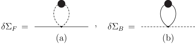
Figure 6: Additional diagrams due to the $\lambda_{4}$ vertex, in the bootstrap equations for the exact propagators.

These diagrams are given by

$$\mathrm{(a)} =-\lambda_{4}\delta_{ji}I\int_{-1/2}^{1/2}du\,\int\!\frac{d^{2}q}{(2\pi)^{2}}\,\frac{1}{\beta}\sum_{n}\frac{1}{\tilde{q}^{2}-\Sigma_{B}(q)}\,,$$ (6.2)

$$\mathrm{(b)} =\lambda_{4}\delta_{ji}\int_{-1/2}^{1/2}du\,\int\!\frac{d^{2}q}{(2\pi)^{2}}\,\frac{1}{\beta}\sum_{n}\mathrm{Tr}_{f}\left(\frac{1}{i\tilde{q}_{\mu}\gamma^{\mu}-\Sigma_{F}(q)}\right)\,.$$ (6.3)

Using the same arguments as in the separate bosonic and fermionic theories, we find again that $\Sigma_{-}=\Sigma_{3}=0$, and that

$$\Sigma_{B}(p) =-\beta^{-2}\mu_{B}^{2}(\lambda)\,,$$ (6.4)

$$\Sigma_{I}(p) =f(y,\lambda)p_{s}\,,$$ (6.5)

$$\Sigma_{+}(p) =g(y,\lambda)p_{+}\,,$$ (6.6)

where

$$g-f^{2}=-\frac{\mu_{F}^{2}(\lambda)}{y^{2}}\,.$$ (6.7)

The diagrams can be computed using the same techniques we used above. Let us define

$$h_{B} \equiv|\lambda|\mu_{B}+\frac{1}{\pi i}\left[\mathrm{Li}_{2}(e^{-\mu_{B}-\pi i|\lambda|})-\mathrm{c.c.}\right]\,,$$ (6.8)

$$h_{F} \equiv|\lambda|\mu_{F}+\frac{1}{\pi i}\left[\mathrm{Li}_{2}(-e^{-\mu_{F}-\pi i|\lambda|})-\mathrm{c.c.}\right]\,.$$ (6.9)

The integrals in (6.2) and (6.3) then evaluate to

$$\int\!du\,\int\!\frac{d^{2}q}{(2\pi)^{2}}\,\frac{1}{\beta}\sum_{n}\frac{1}{\tilde{q}^{2}-\Sigma_{B}(q)} =-\frac{h_{B}}{4\pi\beta|\lambda|}\,,$$ (6.10)

$$\quad\int\!du\, \int\!\frac{d^{2}q}{(2\pi)^{2}}\,\frac{1}{\beta}\sum_{n}\mathrm{Tr}_{f}\left(\frac{1}{i\tilde{q}_{\mu}\gamma^{\mu}-\Sigma_{F}(q)}\right)=$$

$$\quad-\frac{i}{2\pi^{2}\beta^{2}|\lambda|}\int_{0}^{\Lambda^{\prime}}dx\frac{x^{2}f(x)}{\sqrt{x^{2}+\mu_{F}^{2}}}\left[\log\left(\cosh\left(\frac{\sqrt{x^{2}+\mu_{F}^{2}}-\pi i|\lambda|}{2}\right)\right)-\mathrm{c.c.}\right]=$$

$$\quad-\frac{1}{4\pi\beta^{2}\lambda}h_{F}\left(h_{F}-\frac{\lambda_{4}}{2\pi\lambda}h_{B}\right)\,.$$ (6.11)

To compute the last integral in (6.11) we first determined $f(y)$, which using the results of the previous section and (6.10) evaluates to

$$yf(y) =-\lambda\sqrt{y^{2}+\mu_{F}^{2}}+\frac{\mathrm{sign}(\lambda)}{\pi i}\left[\mathrm{Li}_{2}\left(-e^{-\sqrt{y^{2}+\mu_{F}^{2}}+\pi i|\lambda|}\right)-\mathrm{c.c.}\right]+\frac{\lambda_{4}}{4\pi|\lambda|}h_{B}\,.$$ (6.12)

Adding the contributions (6.2) and (6.3) to the bootstrap equations (4.18) and (5.15), we find the corrected equations for the thermal masses,

$$\mu_{B}^{2} =\left(\frac{\hat{\lambda}}{2{\lambda}}h_{B}\right)^{2}+\frac{\lambda_{4}}{4\pi\lambda}h_{F}\left(h_{F}-\frac{\lambda_{4}}{2\pi\lambda}h_{B}\right)\,,$$ (6.13)

$$\mu_{F} =h_{F}-\frac{\lambda_{4}}{4\pi\lambda}h_{B}\,.$$ (6.14)

In the second line we chose the branch that gives a solution with positive $\mu_{F}$.

6.2 Free energy

The free energy receives separate contributions from the scalars and fermions, as well as contributions from the $\lambda_{4}$ interaction. It is given by [4]

$$F=F_{B}+F_{F}+F_{BF}\,,$$ (6.15)

where $F_{B}$ is given (in terms of the self-energy) in (4.25), $F_{F}$ in (5.18), and

$$\beta F_{BF} =-\frac{\lambda_{4}NV_{2}\beta}{6}\left[\int_{-1/2}^{1/2}du\,\int\!\frac{d^{3}q}{(2\pi)^{3}}\,\frac{1}{\tilde{q}^{2}-\Sigma_{B}}\right]\left[\int_{-1/2}^{1/2}du\,\int\!\frac{d^{3}p}{(2\pi)^{3}}\,\mathrm{Tr}_{f}\left(\frac{1}{i\tilde{p}_{\mu}\gamma^{\mu}-\Sigma_{F}}\right)\right]$$

$$=-\frac{NV_{2}}{96\pi^{2}\beta^{2}}\frac{\lambda_{4}}{\lambda|\lambda|}h_{B}h_{F}\left(h_{F}-\frac{\lambda_{4}}{2\pi\lambda}h_{B}\right)\,.$$ (6.16)

In the second line we used the integrals (6.10) and (6.11).

The bosonic contribution $F_{B}$ to the free energy is given by (4.34), and the fermionic contribution can be computed as in section 5.2. The only difference is in equation (5.27), where we must account for the corrected thermal mass equation when computing the integral. We find that

$$\int_{-1/2}^{1/2}du\int\!\frac{d^{2}q}{(2\pi)^{2}}\frac{1}{\beta}\sum_{n=-\infty}^{\infty}\frac{(g-2f^{2})q_{s}^{2}}{\tilde{q}^{2}+\beta^{-2}\mu_{F}^{2}} =\frac{1}{8\pi|\lambda|\beta^{3}}\left\{\frac{1}{3}\left(\frac{\lambda_{4}}{4\pi\lambda}h_{B}\right)^{3}+\frac{1}{3}\left(h_{F}-\frac{\lambda_{4}}{4\pi\lambda}h_{B}\right)^{3}+\mu_{F}^{2}h_{F}\right\}\,.$$ (6.17)

The resulting fermionic contribution to the free energy is

$$\beta F_{F}=\frac{V_{2}N}{2\pi\beta^{2}|\lambda|} \left\{\frac{|\lambda|\mu_{F}^{3}}{3}-\frac{\mu_{F}^{3}}{12}-\frac{\mu_{F}^{2}h_{F}}{4}-\frac{1}{12}\left(\frac{\lambda_{4}}{4\pi\lambda}h_{B}\right)^{3}\right.$$

$$\left.\quad+\frac{1}{\pi i}\int_{\mu_{F}}^{\infty}\!dy\,y\left[\mathrm{Li}_{2}(-e^{-y+\pi i|\lambda|})-\mathrm{c.c.}\right]\right\}\,.$$ (6.18)

Combining all the contributions to the free energy and using (6.8), (6.9) and (6.14) to simplify the expression, we obtain

$$\beta F =-\frac{NV_{2}}{2\pi^{2}i\beta^{2}\lambda}\left\{\frac{\mu_{F}^{2}}{3}\left[\mathrm{Li}_{2}(-e^{-\mu_{F}-\pi i\lambda})-\mathrm{c.c.}\right]-\frac{\mu_{B}^{2}}{3}\left[\mathrm{Li}_{2}(e^{-\mu_{B}-\pi i\lambda})-\mathrm{c.c.}\right]\right.$$

$$\quad\left.+\int_{\mu_{F}}^{\infty}\!dy\,y\left[\mathrm{Li}_{2}(-e^{-y-\pi i\lambda})-\mathrm{c.c.}\right]-\int_{\mu_{B}}^{\infty}\!dy\,y\left[\mathrm{Li}_{2}(e^{-y-\pi i\lambda})-\mathrm{c.c.}\right]\right\}\,.$$ (6.19)

6.3 The supersymmetric case

The theory with $\mathcal{N}=2$ supersymmetry is conjectured to be self-dual [24], with the transformation at large $N$ given by $N\to|k|-N$ and $k\to-k$. In this section we verify that the free energy is invariant under this duality.

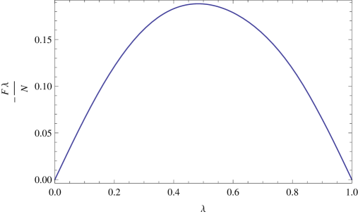
Figure 7: Free energy (times $-\lambda$) in the $\mathcal{N}=2$ theory, in arbitrary normalization.

In this theory, the couplings are given in terms of $\lambda$ by [4]

$$\lambda_{4}=4\pi\lambda\,,\quad\lambda_{6}=24\pi^{2}\lambda^{2}\,,$$ (6.20)

so that $\hat{\lambda}=2|\lambda|$. The equations for the thermal masses become

$$\mu_{B}^{2} =\left(h_{B}-h_{F}\right)^{2}\,,\quad\mu_{F}=h_{F}-h_{B}\,.$$ (6.21)

The thermal masses are therefore equal, $\mu\equiv\mu_{B}=\mu_{F}$, with $\mu$ satisfying

$$\mu =\frac{1}{\pi i}\left[\mathrm{Li}_{2}(e^{-\mu+\pi i|\lambda|})+\mathrm{Li}_{2}(-e^{-\mu-\pi i|\lambda|})-\mathrm{c.c.}\right]\,.$$ (6.22)

The free energy is given by

$$\beta F =\frac{V_{2}N}{2\pi\beta^{2}|\lambda|}\left\{-\frac{\mu^{3}}{3}+\frac{1}{\pi i}\int_{\mu}^{\infty}\!dy\,y\left[\mathrm{Li}_{2}(e^{-y-\pi i|\lambda|})+\mathrm{Li}_{2}(-e^{-y+\pi i|\lambda|})-\mathrm{c.c.}\right]\right\}\,.$$ (6.23)

Both the thermal mass and the free energy are invariant under the duality, which in terms of $N$ and $|\lambda|$ takes $|\lambda|\to 1-|\lambda|$ with $N/|\lambda|$ fixed. The free energy is plotted in figure 7. It is straightforward to generalize our results also to theories with different amounts of supersymmetry, including the theories analyzed in [41, 4].

7 Summary of Results

In this section we collect the main results obtained in this paper.

We have computed the thermal free energy on $\mathbb{R}^{2}$ for various large $N$ vector models coupled to Chern-Simons gauge fields, working exactly in the ‘t Hooft coupling $\lambda=\frac{N}{k}$. In particular, we have explicitly tested the conjectured non-supersymmetric dualities (“3d bosonization”) relating the regular/critical fermion coupled to Chern-Simons to the critical/regular scalar coupled to Chern-Simons [1, 8, 5]. Our calculations closely followed [1, 4, 20], with the difference that we included the effect of the holonomy around the thermal circle, as explained in Section 2.

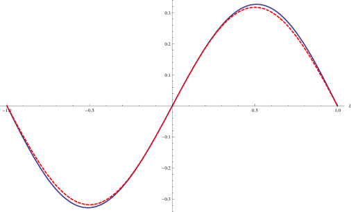
Figure 8: Plot of $(-\lambda)$ times the free energy, $(-\lambda F_{F})$, (blue solid line) and $\lambda$ times the stress-tensor 2-point function $\lambda\langle TT\rangle\sim\frac{\sin\pi\lambda}{\pi}$ (red dashed line) for the regular fermion theory. They look very similar but they have a different functional form.

In all cases we find that the free energy goes to zero at $\lambda=1$, in accordance with the behavior of the exact $\langle TT\rangle$ correlator [5, 6]. In fact, since the thermal free energy $F$ and $\langle TT\rangle$ are both a measure of the number of degrees of freedom of the theory, it is interesting to compare them. Amusingly, we find that their behavior as a function of $\lambda$ is rather similar. As an example, figure 8 shows a plot of $(-\lambda F)$ and $\lambda\langle TT\rangle$ for the regular fermion theory, normalized to agree at weak coupling. Note that it is possible to smoothly continue our results beyond $\lambda=1$. In fact, the functions $\lambda F$ and $\lambda\langle TT\rangle$ in the regular fermion theory (and the critical bosonic theory) are both periodic under $\lambda\to\lambda+2$ and odd under $\lambda\to-\lambda$.

Our results are most simply expressed in terms of the following functions

$$\mathcal{F}(\mu,\lambda) \equiv\frac{1}{2\pi^{2}i}\left[\frac{\mu^{2}}{3}\mathrm{Li}_{2}(e^{-\mu-\pi i\lambda})+\int_{\mu}^{\infty}\!dy\,y\,\mathrm{Li}_{2}(e^{-y-\pi i\lambda})-\mathrm{c.c.}\right]\,,$$ (7.1)

$$h_{B}(\mu_{B},\lambda) \equiv\lambda\mu_{B}+\frac{1}{\pi i}\left[\mathrm{Li}_{2}(e^{-\mu_{B}-\pi i\lambda})-\mathrm{c.c.}\right]\,,$$ (7.2)

$$h_{F}(\mu_{F},\lambda) \equiv\lambda\mu_{F}+\frac{1}{\pi i}\left[\mathrm{Li}_{2}(-e^{-\mu_{F}-\pi i\lambda})-\mathrm{c.c.}\right]\,.$$ (7.3)

7.1 Regular fermion and critical boson results

For the regular fermion theory (a massless fermion coupled to CS), the exact planar free energy takes the form

$$F_{F}=-\frac{NV_{2}T^{3}}{\lambda}\mathcal{F}(\mu_{F},\lambda-{\mathrm{sign}}(\lambda))\,,$$ (7.4)

where the thermal mass $\mu_{F}$ is determined by the equation

$$\mu_{F}=h_{F}(\mu_{F},\lambda)\,.$$ (7.5)

Note that here (unlike our discussion above) we allow $\mu_{F}$ also to be negative, and the equations are still valid in this case. In fact, we have $h_{F}(-\mu_{F},-\lambda)=-h_{F}(\mu_{F},\lambda)$, and the free energy is even under $\lambda\to-\lambda$. For the critical boson coupled to CS, we found

$$F_{B}^{\mathrm{crit.}}=\frac{NV_{2}T^{3}}{\lambda}\mathcal{F}(\mu_{B,c},\lambda)\,,$$ (7.6)

where $\mu_{B,c}$ is given by (again allowing also negative values)

$$h_{B}(\mu_{B,c},\lambda)=0\,,$$ (7.7)

It is now obvious that if the thermal masses map to each other under the duality, so will the free energies. Note that ${N\over\lambda}=k_{\mathrm{YM}}+N\mathrm{sign}(k_{\mathrm{YM}})$ changes sign under the duality It is easy to see that the thermal masses are indeed related by $|\mu_{F}(\lambda)|=|\mu_{B,c}(\lambda-\mathrm{sign}(\lambda))|$, in agreement with the expected duality. The inclusion of the non-trivial holonomy was crucial in order to obtain this.

Our theories have a global $U(1)$ symmetry, which acts on the scalars/fermions in a natural way (the equations of motion of the gauge field identify this symmetry with the topological symmetry of the three dimensional $U(1)$ gauge field). It is simple to generalize our analysis by adding a chemical potential for this gauge field, as done (without taking the holonomy into account) for the regular fermion theory in [42]. In the bosonic theories we find that the effect of adding a chemical potential $\mu_{U(1)}$ is simply to replace every $\mathrm{Li}_{2}(e^{x})$ appearing in our analysis by $\frac{1}{2}(\mathrm{Li}_{2}(e^{x+\mu_{U(1)}})+\mathrm{Li}_{2}(e^{x-\mu_{U(1)}}))$. The chemical potential maps to itself under the duality.

For comparison to results that previously appeared in the literature, one may also look at the perturbative expansion of these results around $\lambda=0$. The first few orders of the thermal mass and free energy for the regular fermion theory read

$$\mu_{F}=2\log(2)\,\lambda+\left(\log^{2}(2)-\frac{\pi^{2}}{12}\right)\lambda^{3}+{\mathcal{O}}(\lambda^{5})\,,$$

$$F_{F}=-NV_{2}T^{3}\left[\frac{3\zeta(3)}{4\pi}-\frac{\pi^{2}\log(2)+4\log^{3}\!(2)}{6\pi}\lambda^{2}+{\mathcal{O}}(\lambda^{4})\right]\,.$$ (7.8)

One may verify that these differ from the results in [1] already at order $\lambda^{2}$. Analogously, one may derive the perturbative expansion of the critical boson free energy. Since the thermal mass $\mu_{B,c}(\lambda=0)=2\log\left(\frac{\sqrt{5}+1}{2}\right)$ is non-zero, the perturbative expansion is analytic. By the duality map, this also means that the expansion of the fermion free energy (and thermal mass) close to $\lambda=1$ is analytic, unlike the result found in [1].

7.2 Regular boson and critical fermion results

In this case, the situation is slightly more complicated due to the possibility of adding a sextic coupling $\frac{\lambda_{6}}{6N^{2}}(J_{0})^{3}$, where $J_{0}$ is the scalar/fermion bilinear. In the large $N$ limit, this coupling is exactly marginal [2] and we have computed the free energies keeping $\lambda_{6}$ as a free parameter. The result for the regular boson turns out to be

$$F_{B}=\frac{NV_{2}T^{3}}{\lambda}\mathcal{F}(\mu_{B},\lambda)\,,$$ (7.9)

where the thermal mass is determined by

$$-\frac{2\lambda}{\hat{\lambda}}\mu_{B}=h_{B}(\mu_{B},\lambda)\,,$$ (7.10)

with $\hat{\lambda}^{2}=\lambda^{2}+\frac{\lambda_{6}}{8\pi^{2}}$.

For the critical fermion theory, we found that the free energy is given by

$$F_{F}^{\mathrm{crit.}}=-\frac{NV_{2}T^{3}}{\lambda}\mathcal{F}(\mu_{F,c},\lambda-{\mathrm{sign}}(\lambda))\,,$$ (7.11)

and the thermal mass is given by

$$(1+\hat{g})\mu_{F,c}=h_{F}(\mu_{F,c},\lambda)\,,$$ (7.12)

where $\hat{g}=1/\sqrt{1-2\pi\lambda\lambda_{6}^{f}}$.

In this case, the duality requires a non-trivial map between the $\lambda_{6}$ couplings, given in equation (5.36), which can be derived independently by matching the scalar three-point functions in the two theories [6]. For example, the critical fermionic theory with $\lambda_{6}^{f}=0$ ($\hat{g}=1$) maps under $\lambda\leftrightarrow\lambda-{\mathrm{sign}}(\lambda)$ to the regular bosonic theory with $\lambda_{6}=24\pi^{2}\lambda^{2}$ ($\hat{\lambda}=2|\lambda|$), as can be easily seen from the expressions above.

7.3 Theories with bosons and fermions

Let us now summarize the results for the theory with one scalar and one fermion, discussed in section 6. This theory contains a boson-fermion coupling $\frac{\lambda_{4}}{N}(\bar{\psi}\psi)(\phi^{{\dagger}}\phi)$ in addition to the scalar sextic coupling $\frac{\lambda_{6}}{6N^{2}}(\phi^{{\dagger}}\phi)^{3}$. We found that the free energy in this theory is

$$F=\frac{NV_{2}T^{3}}{\lambda}\left(\mathcal{F}(\mu_{B},\lambda)-\mathcal{F}(\mu_{F},\lambda-\mathrm{sign}(\lambda))\right)\,,$$ (7.13)

where

$$\mu_{B}^{2} =\left(\frac{\hat{\lambda}}{2\lambda}h_{B}\right)^{2}+\frac{\lambda_{4}}{4\pi\lambda}h_{F}\left(h_{F}-\frac{\lambda_{4}}{2\pi\lambda}h_{B}\right)\,,$$ (7.14)

$$\mu_{F} =h_{F}-\frac{\lambda_{4}}{4\pi\lambda}h_{B}\,,$$ (7.15)

and $\hat{\lambda}$ is defined as in the regular boson theory.

The $\mathcal{N}=2$ supersymmetric Chern-Simons theory with one chiral superfield is a particular case of the above theory, obtained by setting $\hat{\lambda}=2|\lambda|$ and $\lambda_{4}=4\pi\lambda$. In this case we obtain

$$\mu=\mu_{F}=\mu_{B}=h_{F}-h_{B}\,.$$ (7.16)

One finds that $\mu$ is self-dual under the level-rank duality transformation, consistent with the expected Seiberg-like duality of this theory [24].

One would expect that the theory with one scalar and one fermion is self-dual (at infinite $N$) also away from the $\mathcal{N}=2$ supersymmetric point, for general values of $\lambda_{4}$ and $\lambda_{6}$, since we can deform the two theories away from the supersymmetric point, and the deformation is exactly marginal for infinite $N$ (but not for finite $N$). Let us now describe how this duality works in the large $N$ limit.

The single-trace operators of this theory consist of the operators of the regular boson theory, which we will denote by $J_{s}^{b}$ ($s=0,1,\cdots$), and those of the regular fermion theory, denoted by $J_{s}^{f}$. In addition, there is a tower of half-integer spin operators obtained by contracting the scalar with the fermion.

It is easy to generalize the computations of planar correlators of integer spin operators, performed in [5, 6], to this theory. One finds that the results are consistent with conformal invariance for any $\lambda_{4}$ and $\lambda_{6}$. In particular, by computing the exact planar 2-point functions of the operators $(\phi^{{\dagger}}\phi)(\bar{\psi}\psi)$ and $(\phi^{{\dagger}}\phi)^{3}$ we find that these operators have dimension $3+O(1/N)$, consistent with the expectation that these deformations are exactly marginal in the planar limit.

The planar 3-point functions of the operators $J_{s}^{b}$ or $J_{s}^{f}$ with $s\geq 1$ are independent of $\lambda_{4}$ and $\lambda_{6}$, giving the same results as in the regular boson or fermion theories. Therefore the correlators of the currents $J_{s}^{b}$ map to those of $J_{s}^{f}$ under the level-rank transformation. The $\lambda_{4}$ deformation affects planar 3-point functions with insertions of the scalar operators $J_{0}^{b}$ and $J_{0}^{f}$, while $\lambda_{6}$ affects only the 3-point function of $J_{0}^{b}$. By computing 3-point functions with insertions of $J_{0}^{b}$ and $J_{0}^{f}$ we find the duality map of $\lambda_{4}$ and $\lambda_{6}$ to be

$$x_{4}\equiv\frac{\lambda_{4}}{4\pi\lambda} \rightarrow\frac{1}{x_{4}}\,,$$ (7.17)

$$\frac{\hat{\lambda}^{2}}{4\lambda^{2}} \rightarrow\frac{1}{x_{4}^{3}}\left(1+x_{4}^{3}-\frac{\hat{\lambda}^{2}}{4\lambda^{2}}\right)\,.$$ (7.18)

Note that the above transformations are consistent with the self-duality of the $\mathcal{N}=2$ theory in which $x_{4}=\frac{\hat{\lambda}^{2}}{4\lambda^{2}}=1$.

One can now verify that the free energy (7.13) maps to itself under the above transformations for any values of $\lambda_{4}$ and $\lambda_{6}$, consistent with the expected self-duality of this theory. Note that to complete the duality map one has to determine also the mapping of the half-integer spin operators, and include the effects of the additional double-trace deformations of this theory, constructed from the spin $1/2$ operators $(\bar{\psi}\phi)$ and $(\phi^{{\dagger}}\psi)$ (see footnote 11). While the free energy does not depend on those deformations, correlators of the spin $1/2$ operators will. Moreover, one has to prove that all the above deformations are exactly marginal more carefully. We leave a more detailed analysis of these issues to future work.

7.4 Massive theories

While in this paper we have concentrated on the conformal theories, we should note that our results also allow us to readily obtain the thermal free energy for massive fermions or scalars coupled to a Chern-Simons gauge field. Studying these theories in detail is beyond the scope of this paper, but let us make a few brief comments about them.

For example, the regular fermion free energy derived in (5.28), with $\mu_{F}$ obeying (5.16), describes a massive fermion theory, where the mass parameter appearing in the Lagrangian is $m_{F}=\tilde{\sigma}/\beta$. For convenience we rewrite here the two equations defining $\tilde{m}_{f}=\beta m_{f}$,

$${\mathrm{sign}}(\lambda)\mu_{F}=\tilde{m}_{f}+\lambda\mu_{F}+\frac{1}{\pi i}\left[\mathrm{Li}_{2}\left(-e^{-\mu_{F}-\pi i\lambda})-\mathrm{c.c.}\right)\right]\,,$$ (7.19)

$$\beta F_{F} =\frac{NV_{2}}{2\pi\beta^{2}}{1\over\lambda}\left\{\frac{\mu_{F}^{3}}{3}(\lambda-{\mathrm{sign}}(\lambda))+\frac{\tilde{m}_{f}\mu_{F}^{2}}{2}-\frac{{\tilde{m}}_{f}^{3}}{6}+\frac{1}{\pi i}\int_{\mu_{F}}^{\infty}\!dy\,y\left[\mathrm{Li}_{2}\left(-e^{-y+\pi i\lambda}\right)-\mathrm{c.c.}\right]\right\}\,.$$ (7.20)

As above, we allow also negative values of $\mu_{F}$; there is always a solution for either positive or negative $\mu_{F}$.

This theory should be related by the duality to the critical boson theory, with a mass deformation $m_{b}$ proportional to $m_{f}$. In this theory we continue to get equation (4.37), but now we need to add an extra term to the free energy in (4.39) of the form $-{\tilde{m}_{b}\tilde{\sigma}\over 2}$ inside the curly brackets of (4.39) (where again $\tilde{m}_{b}\equiv\beta m_{b}$). The equation for $\tilde{\sigma}$ is now modified into

$${4\over\lambda^{2}}\left(\mu_{B}^{2}-\tilde{\sigma}\right)=\tilde{m}_{b}^{2}\,.$$ (7.21)

Substituting this value of $\tilde{\sigma}$ in (4.37) and (4.39), we obtain (using here $\mu_{B}>0$)

$$-\lambda\tilde{m}_{b}=-\lambda\mu_{B}-\frac{1}{\pi i}\left[\mathrm{Li}_{2}(e^{-\mu_{B}-\pi i\lambda})-\mathrm{Li}_{2}(e^{-\mu_{B}+\pi i\lambda})\right]\,,$$ (7.22)

$$\beta F_{B,m_{b}}^{\mathrm{crit.}}=-\frac{NV_{2}T^{2}}{2\pi}\left\{\frac{\mu_{B}^{3}}{3}+{\lambda^{2}\tilde{m}_{b}^{3}\over 6}-{\tilde{m}_{b}\mu_{B}^{2}\over 2}+\frac{1}{\pi i\lambda}\int_{\mu_{B}}^{\infty}\!dy\,y\left[\mathrm{Li}_{2}(e^{-y+\pi i\lambda})-\mathrm{Li}_{2}(e^{-y-\pi i\lambda})\right]\right\}\,.$$ (7.23)

In writing (7.23) we added to the Lagrangian density a constant term proportional to $N\lambda^{2}m_{b}^{3}$ (this modifies only the second term, and does not affect the physics), in order to match with the fermionic theory, using the identifications

$$|\mu_{B}|=|\mu_{F}|,~{}~{}~{}~{}~{}~{}~{}~{}~{}\lambda_{b}=\lambda_{f}-\mathrm{sign}(\lambda_{f}),~{}~{}~{}~{}~{}~{}~{}\lambda_{b}m_{b}=-m_{f}\,.$$ (7.24)

The last relation between the mass parameters follows (up to a sign) from properly normalizing the associated spin zero operators, using their two-point functions computed in [5, 6].

Actually, this is not precise, since equation (7.22) does not always have a solution (recall $\mu_{B}>0$). When it does not, it turns out that there is (at least at zero temperature [5]) a different configuration in which one of the scalars obtains an expectation value, breaking the $U(N)$ gauge symmetry to $U(N-1)$. The duality implies that analyzing this configuration (using the expectation value that minimizes the free energy) should lead to exactly the same equations that we had above, just for negative values of $\mu_{B}$, in order to be consistent with the matching with the fermionic theory for these values of the mass. It would be interesting to confirm this.

It is interesting to take the zero temperature limit of the above relations. In the zero temperature limit $\tilde{m}$ and $\mu$ become large, so the dilogarithms go to zero if the argument of their exponent is negative (otherwise we can map to this situation, using the identity $\mathrm{Li}_{2}(x)+\mathrm{Li}_{2}(1/x)=-\frac{\pi^{2}}{6}-\frac{1}{2}(\log(-x))^{2}$). For the two theories described above, we find the simple results (assuming for simplicity $0<\lambda_{b}<1$, $-1<\lambda_{f}<0$)

$${\mu_{B}\over\beta}=-{\mu_{F}\over\beta}= m_{b}=-{m_{f}\over(1+\lambda_{f})}~{},~{}~{}~{}~{}~{}~{}~{}~{}~{}~{}~{}~{}~{}\qquad m_{b}>0,m_{f}<0\,,$$ (7.25)

$${\mu_{B}\over\beta}=-{\mu_{F}\over\beta}= {\lambda_{b}m_{b}\over(2-\lambda_{b})}=-{m_{f}\over(1-\lambda_{f})}~{},~{}~{}~{}~{}~{}~{}~{}~{}~{}~{}~{}~{}~{}m_{b}<0,m_{f}>0\,.$$ (7.26)

Note that $\mu_{F,B}/\beta$ is the position of the pole of the dressed fermion/scalar propagator in these theories. This is not a gauge-invariant quantity. However, at least for weak coupling, we expect that the position of this pole is close to the actual physical mass of the lightest (charged) excitation. In the massive theory, the low energy effective description is by a topological pure Chern-Simons theory. We have massive excitations whose worldlines act as Wilson line sources for this Chern-Simons theory, with vanishing forces between them at leading order in the large $N$ limit.

In the fermionic theory for small $\lambda_{f}$ the excitation mass is of order $m_{f}$. However, it seems strange that when $\lambda_{f}$ is not small, we have a significant difference between the two choices of signs for $m_{f}$; the low-energy theories in the two cases differ just by shifting $k$ by one (which is negligible in the large $N$ limit). However, we can understand the origin of this difference by thinking about the critical bosonic theory. In this theory we see that for small $\lambda_{b}$ the physical mass of the excitations is the same as $m_{b}$ for $m_{b}>0$, but is a much smaller scale of order $\lambda_{b}m_{b}$ for negative $m_{b}$. As mentioned in [5], this is because for one sign the theory is in a phase with unbroken $U(N)$, while for the other sign the $U(N)$ symmetry is spontaneously broken to $U(N-1)$ by a scalar vacuum expectation value. Since the $U(N)$ symmetry is gauged, instead of having Nambu-Goldstone bosons, we have light massive gauge bosons with a mass of order $\lambda_{b}m_{b}$ (for $\lambda_{b}\ll 1$).

There is also another way to obtain massive theories. Instead of a massive deformation, in some cases we have (for zero temperature in the regular bosonic and critical fermionic theories) a moduli space along which we can spontaneously break the conformal symmetry by a vacuum expectation value for the gauge-invariant scalar operator. Without the Chern-Simons coupling this possibility was analyzed in [44, 45]. Usually the only solution to our equations at zero temperature is $\mu=0$. However, in our regular bosonic theories, we see that when $\hat{\lambda}=2$ (namely $\lambda^{2}+\frac{\lambda_{6}}{8\pi^{2}}=4$), there is a solution to the “gap equation” (7.10) for the thermal mass for every negative value of $\mu_{B}$ (in the zero temperature limit). This is the manifestation of the opening of a new moduli space of vacua for this specific value of $\hat{\lambda}$ in our analysis. Along this moduli space the conformal symmetry is spontaneously broken, and there is a massless Nambu-Goldstone boson. Of course, for finite temperature this moduli space is lifted, and we also do not expect it to be present for finite values of $N$.

Acknowledgments

We would like to thank S. Banerjee, S. Hellerman, I. Klebanov, J. Maltz, G. Moore, S. Minwalla, M. Moshe, E. Rabinovici, S. Shenker, J. Sonnenschein and X. Yin for useful discussions and correspondence. OA is the Samuel Sebba Professorial Chair of Pure and Applied Physics, and he is supported in part by a grant from the Rosa and Emilio Segre Research Award. The work of OA, GG and RY was supported in part by an Israel Science Foundation center for excellence grant, by the German-Israeli Foundation (GIF) for Scientific Research and Development, and by the Minerva foundation with funding from the Federal German Ministry for Education and Research. OA gratefully acknowledges support from an IBM Einstein Fellowship at the Institute for Advanced Study. The work of JM was supported in part by U.S. Department of Energy grant #DE-FG02-90ER40542.

References

- [1] S. Giombi, S. Minwalla, S. Prakash, S. P. Trivedi, S. R. Wadia and X. Yin, “Chern-Simons Theory with Vector Fermion Matter,” Eur. Phys. J. C 72, 2112 (2012) [arXiv:1110.4386 [hep-th]].
- [2] O. Aharony, G. Gur-Ari and R. Yacoby, “d=3 Bosonic Vector Models Coupled to Chern-Simons Gauge Theories,” JHEP 1203 (2012) 037 [arXiv:1110.4382 [hep-th]].
- [3] C. -M. Chang, S. Minwalla, T. Sharma and X. Yin, “ABJ Triality: from Higher Spin Fields to Strings,” arXiv:1207.4485 [hep-th].
- [4] S. Jain, S. P. Trivedi, S. R. Wadia and S. Yokoyama, “Supersymmetric Chern-Simons Theories with Vector Matter,” arXiv:1207.4750 [hep-th].
- [5] O. Aharony, G. Gur-Ari and R. Yacoby, “Correlation Functions of Large N Chern-Simons-Matter Theories and Bosonization in Three Dimensions,” arXiv:1207.4593 [hep-th].
- [6] G. Gur-Ari and R. Yacoby, “Correlators of Large N Fermionic Chern-Simons Vector Models,” arXiv:1211.1866 [hep-th].
- [7] J. Maldacena and A. Zhiboedov, “Constraining Conformal Field Theories with A Higher Spin Symmetry,” arXiv:1112.1016 [hep-th].
- [8] J. Maldacena and A. Zhiboedov, “Constraining conformal field theories with a slightly broken higher spin symmetry,” arXiv:1204.3882 [hep-th].
- [9] M. A. Vasiliev, “More on equations of motion for interacting massless fields of all spins in (3+1)-dimensions,” Phys. Lett. B 285, 225 (1992).
- [10] M. A. Vasiliev, “Higher spin gauge theories: Star product and AdS space,” In *Shifman, M.A. (ed.): The many faces of the superworld* 533-610 [hep-th/9910096].
- [11] S. Giombi and X. Yin, “The Higher Spin/Vector Model Duality,” arXiv:1208.4036 [hep-th].
- [12] I. R. Klebanov and A. M. Polyakov, “AdS dual of the critical O(N) vector model,” Phys. Lett. B 550, 213 (2002) [hep-th/0210114].
- [13] E. Sezgin and P. Sundell, “Holography in 4D (super) higher spin theories and a test via cubic scalar couplings,” JHEP 0507, 044 (2005) [hep-th/0305040].
- [14] E. Witten, “Quantum Field Theory and the Jones Polynomial,” Commun. Math. Phys. 121, 351 (1989).
- [15] S. G. Naculich, H. A. Riggs and H. J. Schnitzer, “Group Level Duality In Wzw Models And Chern-simons Theory,” Phys. Lett. B 246, 417 (1990).
- [16] M. Camperi, F. Levstein and G. Zemba, “The Large N Limit Of Chern-simons Gauge Theory,” Phys. Lett. B 247, 549 (1990).
- [17] E. J. Mlawer, S. G. Naculich, H. A. Riggs and H. J. Schnitzer, “Group level duality of WZW fusion coefficients and Chern-Simons link observables,” Nucl. Phys. B 352, 863 (1991).
- [18] S. G. Naculich and H. J. Schnitzer, “Level-rank duality of the U(N) WZW model, Chern-Simons theory, and 2-D qYM theory,” JHEP 0706 (2007) 023 [hep-th/0703089].
- [19] A. Kapustin, B. Willett and I. Yaakov, “Tests of Seiberg-like Duality in Three Dimensions,” arXiv:1012.4021 [hep-th].
- [20] O. Aharony, G. Gur-Ari and R. Yacoby, unpublished.
- [21] B. Sundborg, “The Hagedorn transition, deconfinement and N=4 SYM theory,” Nucl. Phys. B 573 (2000) 349 [hep-th/9908001].
- [22] O. Aharony, J. Marsano, S. Minwalla, K. Papadodimas and M. Van Raamsdonk, “The Hagedorn - deconfinement phase transition in weakly coupled large N gauge theories,” Adv. Theor. Math. Phys. 8 (2004) 603 [hep-th/0310285].
- [23] A. Giveon and D. Kutasov, “Seiberg Duality in Chern-Simons Theory,” Nucl. Phys. B 812 (2009) 1 [arXiv:0808.0360 [hep-th]].
- [24] F. Benini, C. Closset and S. Cremonesi, “Comments on 3d Seiberg-like dualities,” JHEP 1110, 075 (2011) [arXiv:1108.5373 [hep-th]].
- [25] O. Aharony, O. Bergman, D. L. Jafferis and J. Maldacena, “N=6 superconformal Chern-Simons-matter theories, M2-branes and their gravity duals,” JHEP 0810 (2008) 091 [arXiv:0806.1218 [hep-th]].
- [26] S. Banerjee, S. Hellerman, J. Maltz and S. H. Shenker, “Light States in Chern-Simons Theory Coupled to Fundamental Matter,” arXiv:1207.4195 [hep-th].
- [27] S. Banerjee, A. Castro, S. Hellerman, E. Hijano, A. Lepage-Jutier, A. Maloney and S. Shenker, “Smoothed Transitions in Higher Spin AdS Gravity,” arXiv:1209.5396 [hep-th].
- [28] A. D. Linde, “Infrared Problem in Thermodynamics of the Yang-Mills Gas,” Phys. Lett. B 96, 289 (1980)..
- [29] B. Svetitsky, “Symmetry Aspects of Finite Temperature Confinement Transitions,” Phys. Rept. 132, 1 (1986).
- [30] E. Braaten and A. Nieto, “Asymptotic behavior of the correlator for Polyakov loops,” Phys. Rev. Lett. 74, 3530 (1995) [hep-ph/9410218].
- [31] E. Brezin, C. Itzykson, G. Parisi and J. B. Zuber, “Planar Diagrams,” Commun. Math. Phys. 59, 35 (1978).
- [32] M. R. Douglas, “Chern-Simons-Witten theory as a topological Fermi liquid,” hep-th/9403119.
- [33] S. Elitzur, G. W. Moore, A. Schwimmer and N. Seiberg, “Remarks on the Canonical Quantization of the Chern-Simons-Witten Theory,” Nucl. Phys. B 326 (1989) 108.
- [34] M. Blau and G. Thompson, “Derivation of the Verlinde formula from Chern-Simons theory and the G/G model,” Nucl. Phys. B 408, 345 (1993) [hep-th/9305010].
- [35] M. Smedback, “On thermodynamics of N=6 superconformal Chern-Simons theory,” JHEP 1004, 002 (2010) [arXiv:1002.0841 [hep-th]].
- [36] S. H. Shenker and X. Yin, “Vector Models in the Singlet Sector at Finite Temperature,” arXiv:1109.3519 [hep-th].
- [37] S. Sachdev, “Polylogarithm identities in a conformal field theory in three-dimensions,” Phys. Lett. B 309, 285 (1993) [hep-th/9305131].
- [38] A. C. Petkou and M. B. Silva Neto, “On the free energy of three-dimensional CFTs and polylogarithms,” Phys. Lett. B 456 (1999) 147 [hep-th/9812166].
- [39] H. R. Christiansen, A. C. Petkou, M. B. Silva Neto and N. D. Vlachos, “On the thermodynamics of the (2+1)-dimensional Gross-Neveu model with complex chemical potential,” Phys. Rev. D 62 (2000) 025018 [hep-th/9911177].
- [40] D. Gaiotto and X. Yin, “Notes on superconformal Chern-Simons-Matter theories,” JHEP 0708, 056 (2007) [arXiv:0704.3740 [hep-th]].
- [41] J. Feinberg, M. Moshe, M. Smolkin and J. Zinn-Justin, “Spontaneous breaking of scale invariance and supersymmetric models at finite temperature,” Int. J. Mod. Phys. A 20 (2005) 4475.
- [42] S. Yokoyama, “Chern-Simons-Fermion Vector Model with Chemical Potential,” arXiv:1210.4109 [hep-th].
- [43] L. V. Avdeev, D. I. Kazakov and I. N. Kondrashuk, “Renormalizations in supersymmetric and nonsupersymmetric nonAbelian Chern-Simons field theories with matter,” Nucl. Phys. B 391 (1993) 333.
- [44] W. A. Bardeen, M. Moshe and M. Bander, “Spontaneous Breaking of Scale Invariance and the Ultraviolet Fixed Point in O() Symmetric in Three-Dimensions) Theory,” Phys. Rev. Lett. 52, 1188 (1984).
- [45] D. J. Amit and E. Rabinovici, “Breaking of scale invariance in phi**6 theory: tricriticality and critical end points,” Nucl. Phys. B 257, 371 (1985).