Unitarising Matrix Element + Parton Shower merging111Work supported in parts by the Swedish research council (contracts 621-2009-4076 and 621-2010-3326).

Leif Lönnblad and Stefan Prestel
Dept. of Astronomy and Theoretical Physics, Lund University, Sweden
E-mail: and
Leif.Lonnblad@thep.lu.se Stefan.Prestel@thep.lu.se
Abstract:

We revisit the CKKW-L method for merging tree-level matrix elements with parton showers, and amend it with an add/subtract scheme to minimise dependencies on the merging scale. The scheme is constructed to, as far as possible, recover the unitary nature of the underlying parton shower, so that the inclusive cross section is retained for each jet multiplicity separately.

QCD, Jets, Parton Model, Phenomenological Models
preprint: LU-TP 12-42
MCnet-12-14
arXiv:1211.4827 [hep-ph] (November 20, 2012)

1 Introduction

Particularly after the discovery of a Higgs-candidate resonance at ATLAS and CMS, the precise description of multi-jet Standard Model (SM) processes at the LHC remains crucial. Major progress has recently been made in combining calculations of next-to-leading order (NLO) perturbative QCD corrections with Parton Shower (PS) based Monte Carlo event generators [1, 2, 3, 4, 5, 6, 7, 8].

In light of the rapid succession of publications on merging multiple NLO calculations with event generators [1, 6, 7, 8], it seems hardly arguable that this long-standing issue is resolved. From the point of next-to-leading order accuracy, scepticism about state-of-the-art methods is baseless. It has however also been pointed out that sub-leading logarithmic enhancements could be left after the merging procedure [9, 10, 11]. It has to be stressed that initially, this problem is not caused by the extension of tree-level methods to NLO, but already appears for CKKW-inspired tree-level merging schemes [12, 13, 14, 15, 16]. The introduction of a merging scale (tMSsubscript𝑡MSt_{\textnormal{\tiny{MS}}}) introduces logarithmic dependencies, L=lnμF/tMS𝐿subscript𝜇𝐹subscript𝑡MSL=\ln\mu_{F}/t_{\textnormal{\tiny{MS}}}, with a dominant contribution αsnL2nsuperscriptsubscript𝛼s𝑛superscript𝐿2𝑛\alpha_{\mathrm{s}}^{n}L^{2n}, in the multi-jet tree-level configurations. These terms are partly cancelled by the parton shower higher-order corrections to low-multiplicity states. Let us look at one-jet merging in WW\mathrm{W}-boson production, with a strictly leading-logarithmic parton shower. Integrating the WW\mathrm{W}+jet matrix element (ME) over the one-jet phase space introduces the dependencies αsL2subscript𝛼ssuperscript𝐿2\alpha_{\mathrm{s}}L^{2} and αsL1subscript𝛼ssuperscript𝐿1\alpha_{\mathrm{s}}L^{1}, while unresolved PS emissions in the zero-jet state produce αsL2subscript𝛼ssuperscript𝐿2\alpha_{\mathrm{s}}L^{2} terms, but with negative sign. In the total cross section, the αsL2subscript𝛼ssuperscript𝐿2\alpha_{\mathrm{s}}L^{2} terms cancel, and only a tMSsubscript𝑡MSt_{\textnormal{\tiny{MS}}}-dependence beyond the accuracy of the parton shower (i.e. αsL1subscript𝛼ssuperscript𝐿1\alpha_{\mathrm{s}}L^{1}-terms) remains. This example is rather academic, since modern parton showers include a matrix-element correction for WW\mathrm{W}+jet production, thus ensuring that in one-jet merging, all dependencies on tMSsubscript𝑡MSt_{\textnormal{\tiny{MS}}} are cancelled222Note that the introduction of ME corrections already endows the PS with the tree-level description of the hardest jet, so that one-jet merging would not be necessary.. After the inclusion of matrix element corrections [17, 18, 19, 20], the merging scale dependence enters for two-jet merging. However, since control of beyond-leading logarithmic contributions cannot be universally exerted in a parton shower, it is clear that dependencies enter at some level, commonly hoped to be at next-to-next-to-leading logarithmic accuracy. The logarithmic structure of a two-jet tree-level cross section for example has only an approximate equivalent in parton showers, meaning that certainly at 𝒪(αs2)𝒪superscriptsubscript𝛼s2\mathcal{O}(\alpha_{\mathrm{s}}^{2}), sub-leading contributions are not fully cancelled. This is often, for lack of a better term, referred to as violation of PS unitarity.

We believe it important to investigate this issue more closely. In this publication, we take a step back from the remarkable progress in NLO merging and outline a tree-level merging method that amends the behaviour of parton showers to ensure that no spurious logarithmic enhancements are introduced by including multi-jet matrix elements. The foundation of this method is PS unitarity, i.e. the requirement that the lowest order cross section remains unchanged by methods introduced to ameliorate the description of shapes of observable. It should be noted that in particular the GKS matrix-element-correction method in VINCIA [21, 22] has emphasised a unitarity-based approach before. The aim of this article is more modest, in that we offer a novel prescription of combining the input used in multi-jet merging procedures, moving from the additive scheme of CKKW-inspired methods to an add-and-subtract method that preserves the total inclusive cross section.

This article is structured as follows. Section 2 is intended as introduction to our perspective on PS unitarity. This will be succeeded by a brief discussion of tree-level merging in the CKKW-L scheme [13, 14, 16] and its problems in section 3, before we move on to construct a LO merging method that preserves PS unitarity in section 4. Section 5 presents results for including additional jets in WW\mathrm{W}-production and QCD dijet processes in the novel procedure, which we call UMEPS (Unitary Matrix Element ++ Parton Shower merging). Finally, we give a discussion in section 6 and conclude in section 7.

2 Parton shower unitarity

Without any outside intervention, parton showers act on a lowest order seed cross section as a unitary operator. In other words, showering dresses the constituents of a perturbatively calculated 22222\to 2 process with radiation, in order to set the stage for hadronisation. By generating soft and collinear emissions, parton showering sums (at least) leading double-logarithmic enhancements to all orders.

Before detailing how this is achieved, let us introduce some notation in order to make the formulae less cluttered. We will also classify partons to be either resolved jets or unresolved jets at a particular scale ρMSsubscript𝜌MS\rho_{\textnormal{\tiny MS}}. By this, we mean that in a jet algorithm that exactly inverts the parton shower, a parton would be resolved as a jet if the evolution scale at which it was emitted (ρ𝜌\rho), as well as jet separations that have been changed by the emission due to recoil effects, are above ρMSsubscript𝜌MS\rho_{\textnormal{\tiny MS}}. For the parton shower to be invertible in a well-defined way, we assume the existence of on-shell intermediate states between splittings. The index MS foreshadows the use of this jet definition as merging scale333 We here restrict ourselves to a particular jet (merging scale) definition, for the sake of clarity. We further assumed that the PS evolution variable is a measure of “hardness”, i.e. that soft and collinear divergences are located at ρ0𝜌0\rho\rightarrow 0. All the following arguments apply for a general merging scale tMSsubscript𝑡MSt_{\textnormal{\tiny{MS}}}..

The parton shower approximates the effect of virtual corrections on observables sensitive to the scales ρisubscript𝜌𝑖\rho_{i} and ρi+1subscript𝜌𝑖1\rho_{i+1} by integrating DGLAP splitting kernels P(z)𝑃𝑧P\left(z\right) over the unresolved phase space. This gives a term

ρi+1ρi𝑑ρ𝑑zαs(ρ)2π{a{outgoing}jPja(z)+a{incoming}jfja(xiaz,ρ)fia(xia,ρ)Pja(z)}subscriptsuperscriptsubscript𝜌𝑖subscript𝜌𝑖1differential-d𝜌differential-d𝑧subscript𝛼s𝜌2𝜋subscript𝑎outgoingsubscript𝑗superscriptsubscript𝑃𝑗𝑎𝑧subscript𝑎incomingsubscript𝑗superscriptsubscript𝑓𝑗𝑎superscriptsubscript𝑥𝑖𝑎𝑧𝜌superscriptsubscript𝑓𝑖𝑎superscriptsubscript𝑥𝑖𝑎𝜌superscriptsubscript𝑃𝑗𝑎𝑧\displaystyle-\int^{\rho_{i}}_{\rho_{i+1}}d\rho~{}dz~{}\frac{\alpha_{\mathrm{s}}(\rho)}{2\pi}\left\{\sum_{a\in\{\textnormal{\tiny{outgoing}}\}}\!\sum_{j}P_{j}^{a}\left(z\right)~{}+\sum_{a\in\{\textnormal{\tiny{incoming}}\}}\!\sum_{j}\frac{f_{j}^{a}(\frac{x_{i}^{a}}{z},\rho)}{f_{i}^{a}(x_{i}^{a},\rho)}P_{j}^{a}\left(z\right)\right\}
ρi+1ρi𝑑ρ𝑑zαs(ρ)𝒫i+1(z,ρ),absentsuperscriptsubscriptsubscript𝜌𝑖1subscript𝜌𝑖differential-d𝜌differential-d𝑧subscript𝛼s𝜌subscript𝒫𝑖1𝑧𝜌\displaystyle\qquad\quad\equiv~{}-\int_{\rho_{i+1}}^{\rho_{i}}\!\!\!d\rho dz\alpha_{\mathrm{s}}\left(\rho\right){\mathcal{P}_{i+1}}\left(z,\rho\right)~{},\quad (1)

where the first terms on the left-hand side sums all possible unresolved final state emissions, and the second term includes all unresolved initial state splittings. The ratios of parton distribution functions f𝑓f is only absent if no initial parton is taking part in the (unresolved) emissions. The 𝒫i+1subscript𝒫𝑖1{\mathcal{P}_{i+1}} (and P𝑃P) notation is rather symbolic to permit a certain degree of simplicity. We include symmetry factors and the typical ρ𝜌\rho- and z𝑧z-fractions from approximating the matrix element or multiplying Jacobian factors in P𝑃P and 𝒫i+1subscript𝒫𝑖1{\mathcal{P}_{i+1}}, e.g. for an initial state splitting q¯q¯g¯q¯qg\bar{\mathrm{q}}\to\bar{\mathrm{q}}\mathrm{g}, we would have P=1ρ1z1+z21z𝑃1𝜌1𝑧1superscript𝑧21𝑧P=\frac{1}{\rho}\frac{1}{z}\frac{1+z^{2}}{1-z}. It can be shown, by performing the z𝑧z-integration for a specific splitting kernel P𝑃P, that the PS “virtual corrections” in eq. (1) indeed capture the leading logarithmic contributions of virtual corrections. Let us introduce the short-hand

fi(xi,ρi)=fi+(xi+,ρi)fi(xi,ρi)subscript𝑓𝑖subscript𝑥𝑖subscript𝜌𝑖superscriptsubscript𝑓𝑖superscriptsubscript𝑥𝑖subscript𝜌𝑖superscriptsubscript𝑓𝑖superscriptsubscript𝑥𝑖subscript𝜌𝑖\displaystyle f_{i}(x_{i},\rho_{i})=f_{i}^{+}(x_{i}^{+},\rho_{i})f_{i}^{-}(x_{i}^{-},\rho_{i}) (2)

The Sudakov form factor, resumming unresolved emissions between scales ρisubscript𝜌𝑖\rho_{i} and ρi+1subscript𝜌𝑖1\rho_{i+1}, is given by

𝚫S+i(xi,ρi,ρi+1)subscript𝚫subscriptSisubscript𝑥𝑖subscript𝜌𝑖subscript𝜌𝑖1\displaystyle{\mathbf{\Delta}_{\mathrm{S_{+i}}}}\left(x_{i},\rho_{i},\rho_{i+1}\right) =\displaystyle= fi(xi,ρi)fi+1(xi,ρi+1)ΠS+i(xi,ρi,ρi+1)subscript𝑓𝑖subscript𝑥𝑖subscript𝜌𝑖subscript𝑓𝑖1subscript𝑥𝑖subscript𝜌𝑖1subscriptΠsubscript𝑆𝑖subscript𝑥𝑖subscript𝜌𝑖subscript𝜌𝑖1\displaystyle\frac{f_{i}(x_{i},\rho_{i})}{f_{i+1}(x_{i},\rho_{i+1})}\Pi_{S_{+i}}\left(x_{i},\rho_{i},\rho_{i+1}\right) (3)

where ΠS+i(xi,ρi,ρi+1)subscriptΠsubscript𝑆𝑖subscript𝑥𝑖subscript𝜌𝑖subscript𝜌𝑖1\Pi_{S_{+i}}\left(x_{i},\rho_{i},\rho_{i+1}\right) is the probability of no emission from state S+isubscript𝑆𝑖S_{+i} between the ρisubscript𝜌𝑖\rho_{i} and ρi+1subscript𝜌𝑖1\rho_{i+1}. The no-emission probability in turn can be expressed as

ΠS+i(xi,ρi,ρi+1)=exp{ρi+1ρi𝑑ρ𝑑zαs(ρ)𝒫i+1(z,ρ)}subscriptΠsubscript𝑆𝑖subscript𝑥𝑖subscript𝜌𝑖subscript𝜌𝑖1superscriptsubscriptsubscript𝜌𝑖1subscript𝜌𝑖differential-d𝜌differential-d𝑧subscript𝛼s𝜌subscript𝒫𝑖1𝑧𝜌\displaystyle\Pi_{S_{+i}}\left(x_{i},\rho_{i},\rho_{i+1}\right)=\exp\left\{-\int_{\rho_{i+1}}^{\rho_{i}}\!\!\!d\rho dz\alpha_{\mathrm{s}}\left(\rho\right){\mathcal{P}_{i+1}}\left(z,\rho\right)\right\} (4)

We have kept xisubscript𝑥𝑖x_{i} as an argument to remember that ΠS+i(xi,ρi,ρi+1)subscriptΠsubscript𝑆𝑖subscript𝑥𝑖subscript𝜌𝑖subscript𝜌𝑖1\Pi_{S_{+i}}\left(x_{i},\rho_{i},\rho_{i+1}\right) contains xisubscript𝑥𝑖x_{i}-dependent PDF factors through 𝒫i+1subscript𝒫𝑖1{\mathcal{P}_{i+1}}.

Let us consider the case when no PS emission above a scale ρMSsubscript𝜌MS\rho_{\textnormal{\tiny MS}} is generated. The parton shower approximation of the resummed exclusive zero-jet cross section is then

dσ0exdϕ0𝑑superscriptsubscript𝜎0𝑒𝑥𝑑subscriptitalic-ϕ0\displaystyle\frac{d\sigma_{0}^{ex}}{d\phi_{0}} =\displaystyle= f0(x0,ρ0)|0(ρ0,μR)|2ΠS+0(x0,ρ0,ρMS)subscript𝑓0subscript𝑥0subscript𝜌0superscriptsubscript0subscript𝜌0subscript𝜇𝑅2subscriptΠsubscript𝑆0subscript𝑥0subscript𝜌0subscript𝜌MS\displaystyle f_{0}(x_{0},\rho_{0})\left|\mathcal{M}_{0}\left(\rho_{0},\mu_{R}\right)\right|^{2}\Pi_{S_{+0}}\left(x_{0},\rho_{0},\rho_{\textnormal{\tiny MS}}\right)
=\displaystyle= f0(x0,ρ0)|0(ρ0,μR)|2subscript𝑓0subscript𝑥0subscript𝜌0superscriptsubscript0subscript𝜌0subscript𝜇𝑅2\displaystyle f_{0}(x_{0},\rho_{0})\left|\mathcal{M}_{0}\left(\rho_{0},\mu_{R}\right)\right|^{2}
\displaystyle- f0(x0,ρ0)|0(ρ0,μR)|2ρMSρ0𝑑ρ𝑑zαs(ρ)𝒫1(z,ρ)subscript𝑓0subscript𝑥0subscript𝜌0superscriptsubscript0subscript𝜌0subscript𝜇𝑅2superscriptsubscriptsubscript𝜌MSsubscript𝜌0differential-d𝜌differential-d𝑧subscript𝛼s𝜌subscript𝒫1𝑧𝜌\displaystyle f_{0}(x_{0},\rho_{0})\left|\mathcal{M}_{0}\left(\rho_{0},\mu_{R}\right)\right|^{2}\int_{\rho_{\textnormal{\tiny MS}}}^{\rho_{0}}\!\!\!d\rho dz\alpha_{\mathrm{s}}\left(\rho\right){\mathcal{P}_{1}}\left(z,\rho\right)
+\displaystyle+ f0(x0,ρ0)|0(ρ0,μR)|2ρMSρ0𝑑ρ1𝑑z1αs(ρ1)𝒫1(z1,ρ1)subscript𝑓0subscript𝑥0subscript𝜌0superscriptsubscript0subscript𝜌0subscript𝜇𝑅2superscriptsubscriptsubscript𝜌MSsubscript𝜌0differential-dsubscript𝜌1differential-dsubscript𝑧1subscript𝛼ssubscript𝜌1subscript𝒫1subscript𝑧1subscript𝜌1\displaystyle f_{0}(x_{0},\rho_{0})\left|\mathcal{M}_{0}\left(\rho_{0},\mu_{R}\right)\right|^{2}\int_{\rho_{\textnormal{\tiny MS}}}^{\rho_{0}}\!\!\!d\rho_{1}dz_{1}\alpha_{\mathrm{s}}\left(\rho_{1}\right){\mathcal{P}_{1}}\left(z_{1},\rho_{1}\right)
×ρMSρ1dρ2dz2αs(ρ2)𝒫1(z2,ρ2)+𝒪(αs3),\displaystyle\qquad\qquad\qquad\qquad\quad~{}\times\int_{\rho_{\textnormal{\tiny MS}}}^{\rho_{1}}\!\!\!d\rho_{2}dz_{2}\alpha_{\mathrm{s}}\left(\rho_{2}\right){\mathcal{P}_{1}}\left(z_{2},\rho_{2}\right)~{}+~{}\mathcal{O}(\alpha_{\mathrm{s}}^{3})~{},

where we have used the fact that

12(ρMSρ0𝑑ρ𝑑zαs(ρ)𝒫1(z,ρ))212superscriptsuperscriptsubscriptsubscript𝜌MSsubscript𝜌0differential-d𝜌differential-d𝑧subscript𝛼s𝜌subscript𝒫1𝑧𝜌2\displaystyle\frac{1}{2}\left(\int_{\rho_{\textnormal{\tiny MS}}}^{\rho_{0}}\!\!\!d\rho dz\alpha_{\mathrm{s}}\left(\rho\right){\mathcal{P}_{1}}\left(z,\rho\right)\right)^{2} (6)
=ρMSρ0𝑑ρ1𝑑z1αs(ρ1)𝒫1(z1,ρ1)ρMSρ1𝑑ρ2𝑑z2αs(ρ2)𝒫1(z2,ρ2).absentsuperscriptsubscriptsubscript𝜌MSsubscript𝜌0differential-dsubscript𝜌1differential-dsubscript𝑧1subscript𝛼ssubscript𝜌1subscript𝒫1subscript𝑧1subscript𝜌1superscriptsubscriptsubscript𝜌MSsubscript𝜌1differential-dsubscript𝜌2differential-dsubscript𝑧2subscript𝛼ssubscript𝜌2subscript𝒫1subscript𝑧2subscript𝜌2\displaystyle=\int_{\rho_{\textnormal{\tiny MS}}}^{\rho_{0}}\!\!\!d\rho_{1}dz_{1}\alpha_{\mathrm{s}}\left(\rho_{1}\right){\mathcal{P}_{1}}\left(z_{1},\rho_{1}\right)\int_{\rho_{\textnormal{\tiny MS}}}^{\rho_{1}}\!\!\!d\rho_{2}dz_{2}\alpha_{\mathrm{s}}\left(\rho_{2}\right){\mathcal{P}_{1}}\left(z_{2},\rho_{2}\right)~{}.

The zero-jet PS cross section is exclusive in the sense that no resolved emissions (i.e. emissions above ρMSsubscript𝜌MS\rho_{\textnormal{\tiny MS}}) are produced. Beside resumming unresolved contributions to the zero-jet cross section, the parton shower also produces resolved emissions. The parton shower approximation to the cross section for emitting the hardest jet at scale ρ1subscript𝜌1\rho_{1} is

dσ1indϕ0𝑑superscriptsubscript𝜎1𝑖𝑛𝑑subscriptitalic-ϕ0\displaystyle\frac{d\sigma_{1}^{in}}{d\phi_{0}} =\displaystyle= dρ1dz1f0(x0,ρ0)|0(ρ0,μR)|2αs(ρ1)𝒫1(z1,ρ1)ΠS+0(x0,ρ0,ρ1).𝑑subscript𝜌1𝑑subscript𝑧1subscript𝑓0subscript𝑥0subscript𝜌0superscriptsubscript0subscript𝜌0subscript𝜇𝑅2subscript𝛼ssubscript𝜌1subscript𝒫1subscript𝑧1subscript𝜌1subscriptΠsubscript𝑆0subscript𝑥0subscript𝜌0subscript𝜌1\displaystyle d\rho_{1}dz_{1}f_{0}(x_{0},\rho_{0})\left|\mathcal{M}_{0}\left(\rho_{0},\mu_{R}\right)\right|^{2}\alpha_{\mathrm{s}}\left(\rho_{1}\right){\mathcal{P}_{1}}\left(z_{1},\rho_{1}\right)\Pi_{S_{+0}}\left(x_{0},\rho_{0},\rho_{1}\right)~{}.

𝒫1subscript𝒫1{\mathcal{P}_{1}} contains PDF ratios and kinematical factors (see definition 1). The cross section is labelled with in𝑖𝑛in for “inclusive”, because the emission of further jets below ρ1subscript𝜌1\rho_{1}, but above ρMSsubscript𝜌MS\rho_{\textnormal{\tiny MS}}, is still allowed. Note that dσ1indϕ0𝑑superscriptsubscript𝜎1𝑖𝑛𝑑subscriptitalic-ϕ0\frac{d\sigma_{1}^{in}}{d\phi_{0}} is also exclusive in the sense that no resolved emissions above ρ1subscript𝜌1\rho_{1} – the scale of the first emission – are possible. In the following, we will always call a cross section inclusive if the parton shower can (at least in principle) produce further resolved emissions, and exclusive otherwise.

If only zero- and one-jet states are generated, the total cross section is given by the sum of exclusive zero-jet and inclusive one-jet cross sections. Let us analyse the total cross section in the approximation of having maximally one parton shower emission. It useful to rewrite eq. (2) with help of definition eq. (4):

dσ0exdϕ0𝑑superscriptsubscript𝜎0𝑒𝑥𝑑subscriptitalic-ϕ0\displaystyle\frac{d\sigma_{0}^{ex}}{d\phi_{0}} =\displaystyle= f0(x0,ρ0)|0(ρ0,μR)|2subscript𝑓0subscript𝑥0subscript𝜌0superscriptsubscript0subscript𝜌0subscript𝜇𝑅2\displaystyle f_{0}(x_{0},\rho_{0})\left|\mathcal{M}_{0}\left(\rho_{0},\mu_{R}\right)\right|^{2}
\displaystyle- f0(x0,ρ0)|0(ρ0,μR)|2ρMSρ0𝑑ρ𝑑zαs(ρ)𝒫1(z,ρ)ΠS+0(x,ρ0,ρ)subscript𝑓0subscript𝑥0subscript𝜌0superscriptsubscript0subscript𝜌0subscript𝜇𝑅2superscriptsubscriptsubscript𝜌MSsubscript𝜌0differential-d𝜌differential-d𝑧subscript𝛼s𝜌subscript𝒫1𝑧𝜌subscriptΠsubscript𝑆0𝑥subscript𝜌0𝜌\displaystyle f_{0}(x_{0},\rho_{0})\left|\mathcal{M}_{0}\left(\rho_{0},\mu_{R}\right)\right|^{2}\int_{\rho_{\textnormal{\tiny MS}}}^{\rho_{0}}\!\!\!d\rho dz\alpha_{\mathrm{s}}\left(\rho\right){\mathcal{P}_{1}}\left(z,\rho\right)\Pi_{S_{+0}}\left(x,\rho_{0},\rho\right)

so that the total cross section is

σinsuperscript𝜎𝑖𝑛\displaystyle\sigma^{in} =\displaystyle= 𝑑ϕ0(dσ0exdϕ0+dσ1indϕ0)differential-dsubscriptitalic-ϕ0𝑑superscriptsubscript𝜎0𝑒𝑥𝑑subscriptitalic-ϕ0𝑑superscriptsubscript𝜎1𝑖𝑛𝑑subscriptitalic-ϕ0\displaystyle\int d\phi_{0}\left(\frac{d\sigma_{0}^{ex}}{d\phi_{0}}+\int\frac{d\sigma_{1}^{in}}{d\phi_{0}}\right) (8)
=\displaystyle= dϕ0(f0(x0,ρ0)|0(ρ0,μR)|2\displaystyle\int d\phi_{0}\Bigg{(}f_{0}(x_{0},\rho_{0})\left|\mathcal{M}_{0}\left(\rho_{0},\mu_{R}\right)\right|^{2}
f0(x0,ρ0)|0(ρ0,μR)|2ρMSρ0dρdzαs(ρ)𝒫1(z,ρ)ΠS+0(x,ρ0,ρ))\displaystyle\quad~{}-~{}f_{0}(x_{0},\rho_{0})\left|\mathcal{M}_{0}\left(\rho_{0},\mu_{R}\right)\right|^{2}\int_{\rho_{\textnormal{\tiny MS}}}^{\rho_{0}}\!\!\!d\rho dz\alpha_{\mathrm{s}}\left(\rho\right){\mathcal{P}_{1}}\left(z,\rho\right)\Pi_{S_{+0}}\left(x,\rho_{0},\rho\right)\Bigg{)}
+\displaystyle+ 𝑑ϕ0f0(x0,ρ0)|0(ρ0,μR)|2ρMSρ0𝑑ρ𝑑zαs(ρ)𝒫(z,ρ)ΠS+0(x0,ρ0,ρ)differential-dsubscriptitalic-ϕ0subscript𝑓0subscript𝑥0subscript𝜌0superscriptsubscript0subscript𝜌0subscript𝜇𝑅2superscriptsubscriptsubscript𝜌MSsubscript𝜌0differential-d𝜌differential-d𝑧subscript𝛼s𝜌𝒫𝑧𝜌subscriptΠsubscript𝑆0subscript𝑥0subscript𝜌0𝜌\displaystyle\int d\phi_{0}f_{0}(x_{0},\rho_{0})\left|\mathcal{M}_{0}\left(\rho_{0},\mu_{R}\right)\right|^{2}\int_{\rho_{\textnormal{\tiny MS}}}^{\rho_{0}}\!\!\!d\rho dz\alpha_{\mathrm{s}}\left(\rho\right){\mathcal{P}}\left(z,\rho\right)\Pi_{S_{+0}}\left(x_{0},\rho_{0},\rho\right)
=\displaystyle= 𝑑ϕ0f0(x0,ρ0)|0(ρ0,μR)|2differential-dsubscriptitalic-ϕ0subscript𝑓0subscript𝑥0subscript𝜌0superscriptsubscript0subscript𝜌0subscript𝜇𝑅2\displaystyle\int d\phi_{0}f_{0}(x_{0},\rho_{0})\left|\mathcal{M}_{0}\left(\rho_{0},\mu_{R}\right)\right|^{2}

Thus, if the parton shower would stop after the first emission, the total cross section is not changed by the application of the parton shower.

This small sketch does not really ensure that the total cross section is preserved after PS resummation. Parton showering usually generates more than one emission, so that only being concerned with a single emission might not be enough. The above argument can however be extended to any number of emissions. As an example, assume the PS had generated two emissions. Then, the one-jet cross section becomes exclusive by demanding that only one resolved emission has been produced,

dσ1exdϕ0𝑑superscriptsubscript𝜎1𝑒𝑥𝑑subscriptitalic-ϕ0\displaystyle\frac{d\sigma_{1}^{ex}}{d\phi_{0}} =\displaystyle= dρ1dz1f0(x0,ρ0)|0(ρ0,μR)|2𝑑subscript𝜌1𝑑subscript𝑧1subscript𝑓0subscript𝑥0subscript𝜌0superscriptsubscript0subscript𝜌0subscript𝜇𝑅2\displaystyle d\rho_{1}dz_{1}f_{0}(x_{0},\rho_{0})\left|\mathcal{M}_{0}\left(\rho_{0},\mu_{R}\right)\right|^{2} (9)
αs(ρ1)𝒫1(z1,ρ1)ΠS+0(x0,ρ0,ρ1)ΠS+1(x1,ρ1,ρMS)subscript𝛼ssubscript𝜌1subscript𝒫1subscript𝑧1subscript𝜌1subscriptΠsubscript𝑆0subscript𝑥0subscript𝜌0subscript𝜌1subscriptΠsubscript𝑆1subscript𝑥1subscript𝜌1subscript𝜌MS\displaystyle\alpha_{\mathrm{s}}\left(\rho_{1}\right){\mathcal{P}_{1}}\left(z_{1},\rho_{1}\right)\Pi_{S_{+0}}\left(x_{0},\rho_{0},\rho_{1}\right)\Pi_{S_{+1}}\left(x_{1},\rho_{1},\rho_{\textnormal{\tiny MS}}\right)

and we need to add the PS approximation to the two-jet cross section

dσ2indϕ0𝑑superscriptsubscript𝜎2𝑖𝑛𝑑subscriptitalic-ϕ0\displaystyle\frac{d\sigma_{2}^{in}}{d\phi_{0}} =\displaystyle= dρ1dz1dρ2dz2f0(x0,ρ0)|0(ρ0,μR)|2𝑑subscript𝜌1𝑑subscript𝑧1𝑑subscript𝜌2𝑑subscript𝑧2subscript𝑓0subscript𝑥0subscript𝜌0superscriptsubscript0subscript𝜌0subscript𝜇𝑅2\displaystyle d\rho_{1}dz_{1}d\rho_{2}dz_{2}f_{0}(x_{0},\rho_{0})\left|\mathcal{M}_{0}\left(\rho_{0},\mu_{R}\right)\right|^{2} (10)
×αs(ρ1)𝒫1(z1,ρ1)ΠS+0(x0,ρ0,ρ1)absentsubscript𝛼ssubscript𝜌1subscript𝒫1subscript𝑧1subscript𝜌1subscriptΠsubscript𝑆0subscript𝑥0subscript𝜌0subscript𝜌1\displaystyle\times~{}\alpha_{\mathrm{s}}\left(\rho_{1}\right){\mathcal{P}_{1}}\left(z_{1},\rho_{1}\right)\Pi_{S_{+0}}\left(x_{0},\rho_{0},\rho_{1}\right)
×αs(ρ2)𝒫2(z2,ρ2)ΠS+1(x1,ρ1,ρ2)Θ(ρ1ρ2)absentsubscript𝛼ssubscript𝜌2subscript𝒫2subscript𝑧2subscript𝜌2subscriptΠsubscript𝑆1subscript𝑥1subscript𝜌1subscript𝜌2Θsubscript𝜌1subscript𝜌2\displaystyle\times~{}\alpha_{\mathrm{s}}\left(\rho_{2}\right){\mathcal{P}_{2}}\left(z_{2},\rho_{2}\right)\Pi_{S_{+1}}\left(x_{1},\rho_{1},\rho_{2}\right)\Theta\left(\rho_{1}-\rho_{2}\right)

Now we rewrite 9 by expanding the second no-emission probability

dσ1exdϕ0𝑑superscriptsubscript𝜎1𝑒𝑥𝑑subscriptitalic-ϕ0\displaystyle\frac{d\sigma_{1}^{ex}}{d\phi_{0}} =\displaystyle= dρ1dz1f0(x0,ρ0)|0(ρ0,μR)|2αs(ρ1)𝒫1(z1,ρ1)ΠS+0(x0,ρ0,ρ1)𝑑subscript𝜌1𝑑subscript𝑧1subscript𝑓0subscript𝑥0subscript𝜌0superscriptsubscript0subscript𝜌0subscript𝜇𝑅2subscript𝛼ssubscript𝜌1subscript𝒫1subscript𝑧1subscript𝜌1subscriptΠsubscript𝑆0subscript𝑥0subscript𝜌0subscript𝜌1\displaystyle d\rho_{1}dz_{1}f_{0}(x_{0},\rho_{0})\left|\mathcal{M}_{0}\left(\rho_{0},\mu_{R}\right)\right|^{2}\alpha_{\mathrm{s}}\left(\rho_{1}\right){\mathcal{P}_{1}}\left(z_{1},\rho_{1}\right)\Pi_{S_{+0}}\left(x_{0},\rho_{0},\rho_{1}\right)
×(1ρMSρ1dρ2dz2αs(ρ2)𝒫2(z2,ρ2)\displaystyle\times~{}\Bigg{(}1-\int_{\rho_{\textnormal{\tiny MS}}}^{\rho_{1}}\!\!\!d\rho_{2}dz_{2}\alpha_{\mathrm{s}}\left(\rho_{2}\right){\mathcal{P}_{2}}\left(z_{2},\rho_{2}\right)
+ρMSρ1dρ2dz2ρMSρ2dρ3dz3αs(ρ3)𝒫2(z3,ρ3)+𝒪(αs3))\displaystyle\quad~{}+\int_{\rho_{\textnormal{\tiny MS}}}^{\rho_{1}}\!\!\!d\rho_{2}dz_{2}\int_{\rho_{\textnormal{\tiny MS}}}^{\rho_{2}}\!\!\!d\rho_{3}dz_{3}\alpha_{\mathrm{s}}\left(\rho_{3}\right){\mathcal{P}_{2}}\left(z_{3},\rho_{3}\right)+\mathcal{O}(\alpha_{\mathrm{s}}^{3})\Bigg{)}
=\displaystyle= dρ1dz1f0(x0,ρ0)|0(ρ0,μR)|2αs(ρ1)𝒫1(z1,ρ1)ΠS+0(x0,ρ0,ρ1)𝑑subscript𝜌1𝑑subscript𝑧1subscript𝑓0subscript𝑥0subscript𝜌0superscriptsubscript0subscript𝜌0subscript𝜇𝑅2subscript𝛼ssubscript𝜌1subscript𝒫1subscript𝑧1subscript𝜌1subscriptΠsubscript𝑆0subscript𝑥0subscript𝜌0subscript𝜌1\displaystyle d\rho_{1}dz_{1}f_{0}(x_{0},\rho_{0})\left|\mathcal{M}_{0}\left(\rho_{0},\mu_{R}\right)\right|^{2}\alpha_{\mathrm{s}}\left(\rho_{1}\right){\mathcal{P}_{1}}\left(z_{1},\rho_{1}\right)\Pi_{S_{+0}}\left(x_{0},\rho_{0},\rho_{1}\right)
×(1ρMSρ1𝑑ρ𝑑zαs(ρ)𝒫2(z,ρ)ΠS+1(x1,ρ1,ρ))absent1superscriptsubscriptsubscript𝜌MSsubscript𝜌1differential-d𝜌differential-d𝑧subscript𝛼s𝜌subscript𝒫2𝑧𝜌subscriptΠsubscript𝑆1subscript𝑥1subscript𝜌1𝜌\displaystyle\times~{}\Bigg{(}1-\int_{\rho_{\textnormal{\tiny MS}}}^{\rho_{1}}\!\!\!d\rho dz\alpha_{\mathrm{s}}\left(\rho\right){\mathcal{P}_{2}}\left(z,\rho\right)\Pi_{S_{+1}}\left(x_{1},\rho_{1},\rho\right)\Bigg{)}

where we have again used definition 4 to derive the last equality. If parton showering stops after generating maximally two emissions, the total cross section is given by

σinsuperscript𝜎𝑖𝑛\displaystyle\sigma^{in} =\displaystyle= 𝑑ϕ0(dσ0exdϕ0+dσ1exdϕ0+dσ2indϕ0)differential-dsubscriptitalic-ϕ0𝑑superscriptsubscript𝜎0𝑒𝑥𝑑subscriptitalic-ϕ0𝑑superscriptsubscript𝜎1𝑒𝑥𝑑subscriptitalic-ϕ0𝑑superscriptsubscript𝜎2𝑖𝑛𝑑subscriptitalic-ϕ0\displaystyle\int d\phi_{0}\left(\frac{d\sigma_{0}^{ex}}{d\phi_{0}}+\int\frac{d\sigma_{1}^{ex}}{d\phi_{0}}+\int\int\frac{d\sigma_{2}^{in}}{d\phi_{0}}\right) (12)

By comparing the second term in eq. (2) with eq. (10), we see that any PS contribution of two resolved jets cancels with terms containing one resolved and one unresolved jet. Already earlier, we saw that contributions with one resolved jet cancel against terms with zero resolved jets. Thus, we again find

σin=𝑑ϕ0f0(x0,ρ0)|0(ρ0,μR)|2superscript𝜎𝑖𝑛differential-dsubscriptitalic-ϕ0subscript𝑓0subscript𝑥0subscript𝜌0superscriptsubscript0subscript𝜌0subscript𝜇𝑅2\displaystyle\sigma^{in}=\int d\phi_{0}f_{0}(x_{0},\rho_{0})\left|\mathcal{M}_{0}\left(\rho_{0},\mu_{R}\right)\right|^{2}

It is easy to extend this argument to as many emissions as wanted: Whenever the parton shower generates one emission, the change in the total cross section is counteracted exactly by unresolved contributions to states with one emission less. There is no need to correct the PS approximation of the zero-jet exclusive cross section in the presence of two-jet states – the zero-jet resummation is oblivious of two-jet states. That parton showers are unitary is understandable directly from their construction, since the branching of an underlying n𝑛n-jet state produces a n+1𝑛1n+1-jet state, which overwrites (i.e. removes) the n𝑛n-jet state in the wake of the branching.

3 The problem with CKKW-L

Let us now review tree-level matrix element merging, more specifically the CKKW-L scheme444Although most of what we discuss also applies to other CKKW-inspired merging schemes.. We here focus mainly on issues related to parton shower unitarity, and refer to [16] for a detailed description of CKKW-L in PYTHIA8 [23] and to [12, 13, 14, 15] for a more general introduction.

Matrix element merging procedures are designed to improve the PS description of multi-jet observables. For this purpose, tree-level matrix element (ME) calculations are combined with the parton shower, i.e. tree-level-weighted phase space points with m𝑚m “hard process particles” and n𝑛n additional partons are included in the shower. In the following, we will often use the terms state, event, configuration or the symbol S+nsubscript𝑆𝑛S_{+n} to refer to these n+m𝑛limit-from𝑚n+m-body phase space points. As can be inferred from the form of S+nsubscript𝑆𝑛S_{+n}, we will most often understand that the state contains m𝑚m hard process particles, but not mention these particles explicitly.

A consistent merging removes all overlap between ME states and the PS approximation. This is ensured by introducing a phase space cut ρMSsubscript𝜌MS\rho_{\textnormal{\tiny MS}} to separate the ME region from the PS region, and applying no-emission probabilities. The cut dependence is minimised by weighting configurations above and below ρMSsubscript𝜌MS\rho_{\textnormal{\tiny MS}} in identical fashion. The CKKW-L scheme constructs and chooses a sequence of lower-multiplicity states (a so-called parton shower history) for each ME event, since factors need to be generated that would, in the parton shower evolution, have contributed though intermediate stages. With the help of the history, ME events will be reweighted with

wnsubscript𝑤𝑛\displaystyle w_{n} =\displaystyle= x0f0(x0,ρ0)xnfn(xn,μF)×(i=1nxifi(xi,ρi)xi1fi1(xi1,ρi))subscript𝑥0subscript𝑓0subscript𝑥0subscript𝜌0subscript𝑥𝑛subscript𝑓𝑛subscript𝑥𝑛subscript𝜇𝐹superscriptsubscriptproduct𝑖1𝑛subscript𝑥𝑖subscript𝑓𝑖subscript𝑥𝑖subscript𝜌𝑖subscript𝑥𝑖1subscript𝑓𝑖1subscript𝑥𝑖1subscript𝜌𝑖\displaystyle\frac{x_{0}f_{0}(x_{0},\rho_{0})}{x_{n}f_{n}(x_{n},\mu_{F})}\times\left(\prod_{i=1}^{n}\frac{x_{i}f_{i}(x_{i},\rho_{i})}{x_{i-1}f_{i-1}(x_{i-1},\rho_{i})}\right) (14)
×(i=1nαs(ρi)αs(μR))×(i=1nΠS+i1(ρi1,ρi))×ΠS+n(ρn,ρMS)absentsuperscriptsubscriptproduct𝑖1𝑛subscript𝛼ssubscript𝜌𝑖subscript𝛼ssubscript𝜇𝑅superscriptsubscriptproduct𝑖1𝑛subscriptΠsubscript𝑆𝑖1subscript𝜌𝑖1subscript𝜌𝑖subscriptΠsubscript𝑆𝑛subscript𝜌𝑛subscript𝜌MS\displaystyle\times\left(\prod_{i=1}^{n}\tfrac{\alpha_{\mathrm{s}}(\rho_{i})}{\alpha_{\mathrm{s}}(\mu_{R})}\right)\times\left(\prod_{i=1}^{n}\Pi_{S_{+i-1}}(\rho_{i-1},\rho_{i})\right)\times\Pi_{S_{+n}}(\rho_{n},\rho_{\textnormal{\tiny MS}})
=\displaystyle= xnfn(xn,ρn)xnfn(xn,μF)×i=1n[αs(ρi)αsMExi1fi1(xi1,ρi1)xi1fi1(xi1,ρi)ΠS+i1(xi1,ρi1,ρi)]subscript𝑥𝑛subscript𝑓𝑛subscript𝑥𝑛subscript𝜌𝑛subscript𝑥𝑛subscript𝑓𝑛subscript𝑥𝑛subscript𝜇𝐹superscriptsubscriptproduct𝑖1𝑛delimited-[]subscript𝛼ssubscript𝜌𝑖subscript𝛼sMEsubscript𝑥𝑖1subscript𝑓𝑖1subscript𝑥𝑖1subscript𝜌𝑖1subscript𝑥𝑖1subscript𝑓𝑖1subscript𝑥𝑖1subscript𝜌𝑖subscriptΠsubscript𝑆𝑖1subscript𝑥𝑖1subscript𝜌𝑖1subscript𝜌𝑖\displaystyle~{}\frac{x_{n}f_{n}(x_{n},\rho_{n})}{x_{n}f_{n}(x_{n},\mu_{F})}~{}\times~{}\prod_{i=1}^{n}\Bigg{[}~{}\frac{\alpha_{\mathrm{s}}(\rho_{i})}{\alpha_{\textnormal{s\tiny{ME}}}}\frac{x_{i-1}f_{i-1}(x_{i-1},\rho_{i-1})}{x_{i-1}f_{i-1}(x_{i-1},\rho_{i})}\Pi_{S_{+i-1}}(x_{i-1},\rho_{i-1},\rho_{i})~{}\Bigg{]}
×ΠS+n(xn,ρn,ρMS),absentsubscriptΠsubscript𝑆𝑛subscript𝑥𝑛subscript𝜌𝑛subscript𝜌MS\displaystyle\times~{}\Pi_{S_{+n}}(x_{n},\rho_{n},\rho_{\textnormal{\tiny MS}})~{},

where ρisubscript𝜌𝑖\rho_{i} are the reconstructed splitting scales, and S+isubscript𝑆𝑖S_{+i} the reconstructed intermediate states. The first PDF ratio in eq. (14) ensures that all ME configurations are normalised to the same total cross section, given by the lowest order Born-level matrix element. The PDF ratios in brackets account for PDF factors in the shower splitting probabilities 𝒫isubscript𝒫𝑖{\mathcal{P}_{i}} for initial state backward evolution. The running of αssubscript𝛼s\alpha_{\mathrm{s}} is correctly included by the second bracket. Finally, double-counting is prevented by multiplying no-emission probabilities.

Let us investigate how the CKKW-L merging prescription changes the lowest-order inclusive cross section. For simplicity, we will highlight merging matrix elements with up to two additional jets with parton showers. In the simplest conceivable case of one-jet merging, applying CKKW-L defines the cross sections

dσ0exdϕ0𝑑superscriptsubscript𝜎0𝑒𝑥𝑑subscriptitalic-ϕ0\displaystyle\frac{d\sigma_{0}^{ex}}{d\phi_{0}} =\displaystyle= f0(x0,ρ0)|0(ρ0,μR)|2ΠS+0(x0,ρ0,ρMS)subscript𝑓0subscript𝑥0subscript𝜌0superscriptsubscript0subscript𝜌0subscript𝜇𝑅2subscriptΠsubscript𝑆0subscript𝑥0subscript𝜌0subscript𝜌MS\displaystyle f_{0}(x_{0},\rho_{0})\left|\mathcal{M}_{0}\left(\rho_{0},\mu_{R}\right)\right|^{2}\Pi_{S_{+0}}\left(x_{0},\rho_{0},\rho_{\textnormal{\tiny MS}}\right)
=\displaystyle= f0(x0,ρ0)|0(ρ0,μR)|2×(1ρMSρ0𝑑ρ𝑑zαs(ρ)𝒫1(z,ρ)+𝒪(αs2))subscript𝑓0subscript𝑥0subscript𝜌0superscriptsubscript0subscript𝜌0subscript𝜇𝑅21superscriptsubscriptsubscript𝜌MSsubscript𝜌0differential-d𝜌differential-d𝑧subscript𝛼s𝜌subscript𝒫1𝑧𝜌𝒪superscriptsubscript𝛼s2\displaystyle f_{0}(x_{0},\rho_{0})\left|\mathcal{M}_{0}\left(\rho_{0},\mu_{R}\right)\right|^{2}\times\Bigg{(}1-\int_{\rho_{\textnormal{\tiny MS}}}^{\rho_{0}}\!\!\!d\rho dz\alpha_{\mathrm{s}}\left(\rho\right){\mathcal{P}_{1}}\left(z,\rho\right)+\mathcal{O}(\alpha_{\mathrm{s}}^{2})\Bigg{)}
dσ1indϕ0𝑑superscriptsubscript𝜎1𝑖𝑛𝑑subscriptitalic-ϕ0\displaystyle\frac{d\sigma_{1}^{in}}{d\phi_{0}} =\displaystyle= dρ1dz1f0(x0,ρ0)αs(ρ1)αs(μR)f1(x1,ρ1)f0(x0,ρ1)|1(ρ0,μR)|2ΠS+0(x0,ρ0,ρ1)𝑑subscript𝜌1𝑑subscript𝑧1subscript𝑓0subscript𝑥0subscript𝜌0subscript𝛼ssubscript𝜌1subscript𝛼ssubscript𝜇𝑅subscript𝑓1subscript𝑥1subscript𝜌1subscript𝑓0subscript𝑥0subscript𝜌1superscriptsubscript1subscript𝜌0subscript𝜇𝑅2subscriptΠsubscript𝑆0subscript𝑥0subscript𝜌0subscript𝜌1\displaystyle d\rho_{1}dz_{1}f_{0}(x_{0},\rho_{0})\frac{\alpha_{\mathrm{s}}(\rho_{1})}{\alpha_{\mathrm{s}}(\mu_{R})}\frac{f_{1}(x_{1},\rho_{1})}{f_{0}(x_{0},\rho_{1})}\left|\mathcal{M}_{1}\left(\rho_{0},\mu_{R}\right)\right|^{2}\Pi_{S_{+0}}\left(x_{0},\rho_{0},\rho_{1}\right) (16)

It is crucial to note that the tree-level one-jet matrix element is in general different from the approximate PS splitting kernels. The inclusive lowest-order cross section is only preserved if

f0(x0,ρ0)|0(ρ0,μR)|2ρMSρ0𝑑ρ𝑑zαs(ρ)𝒫1(z,ρ)subscript𝑓0subscript𝑥0subscript𝜌0superscriptsubscript0subscript𝜌0subscript𝜇𝑅2superscriptsubscriptsubscript𝜌MSsubscript𝜌0differential-d𝜌differential-d𝑧subscript𝛼s𝜌subscript𝒫1𝑧𝜌\displaystyle f_{0}(x_{0},\rho_{0})\left|\mathcal{M}_{0}\left(\rho_{0},\mu_{R}\right)\right|^{2}\int_{\rho_{\textnormal{\tiny MS}}}^{\rho_{0}}\!\!\!d\rho dz\alpha_{\mathrm{s}}\left(\rho\right){\mathcal{P}_{1}}\left(z,\rho\right) (17)
=ρMSρ0𝑑ρ1𝑑z1f0(x0,ρ0)αs(ρ1)αs(μR)f1(x1,ρ1)f0(x0,ρ1)|1(ρ0,μR)|2,absentsuperscriptsubscriptsubscript𝜌MSsubscript𝜌0differential-dsubscript𝜌1differential-dsubscript𝑧1subscript𝑓0subscript𝑥0subscript𝜌0subscript𝛼ssubscript𝜌1subscript𝛼ssubscript𝜇𝑅subscript𝑓1subscript𝑥1subscript𝜌1subscript𝑓0subscript𝑥0subscript𝜌1superscriptsubscript1subscript𝜌0subscript𝜇𝑅2\displaystyle=\int_{\rho_{\textnormal{\tiny MS}}}^{\rho_{0}}\!\!\!d\rho_{1}dz_{1}f_{0}(x_{0},\rho_{0})\frac{\alpha_{\mathrm{s}}(\rho_{1})}{\alpha_{\mathrm{s}}(\mu_{R})}\frac{f_{1}(x_{1},\rho_{1})}{f_{0}(x_{0},\rho_{1})}\left|\mathcal{M}_{1}\left(\rho_{0},\mu_{R}\right)\right|^{2}~{},

i.e. in the case where the first parton shower emission is distributed exactly according the one-jet matrix element. In this case, we would not have needed a merging prescription, since the PS would have already produced the correct result.

Though correcting the first PS splitting to the full tree-level result is reasonably simple, correcting higher multiplicities requires significantly more work. The VINCIA program aims at solving this issue [21, 22]. In general however, we are currently forced to rely on tree-level merging to improve the descriptions of multi-jet observables.

If a first-splitting-corrected PS is available, unitarity violations will enter when including matrix elements for the next higher jet multiplicity. Since the case of two-jet merging is also instructive for later considerations, we will list the contributions to the cross section below.

dσ0exdϕ0𝑑superscriptsubscript𝜎0𝑒𝑥𝑑subscriptitalic-ϕ0\displaystyle\frac{d\sigma_{0}^{ex}}{d\phi_{0}} =\displaystyle= f0(x0,ρ0)|0(ρ0,μR)|2ΠS+0(x0,ρ0,ρMS)subscript𝑓0subscript𝑥0subscript𝜌0superscriptsubscript0subscript𝜌0subscript𝜇𝑅2subscriptΠsubscript𝑆0subscript𝑥0subscript𝜌0subscript𝜌MS\displaystyle f_{0}(x_{0},\rho_{0})\left|\mathcal{M}_{0}\left(\rho_{0},\mu_{R}\right)\right|^{2}\Pi_{S_{+0}}\left(x_{0},\rho_{0},\rho_{\textnormal{\tiny MS}}\right) (18)
=\displaystyle= f0(x0,ρ0)|0(ρ0,μR)|2subscript𝑓0subscript𝑥0subscript𝜌0superscriptsubscript0subscript𝜌0subscript𝜇𝑅2\displaystyle f_{0}(x_{0},\rho_{0})\left|\mathcal{M}_{0}\left(\rho_{0},\mu_{R}\right)\right|^{2}
×(1ρMSρ0𝑑ρ𝑑zαs(ρ)𝒫1(z,ρ)ΠS+0(x0,ρ0,ρ))absent1superscriptsubscriptsubscript𝜌MSsubscript𝜌0differential-d𝜌differential-d𝑧subscript𝛼s𝜌subscript𝒫1𝑧𝜌subscriptΠsubscript𝑆0subscript𝑥0subscript𝜌0𝜌\displaystyle\times\left(1-\int_{\rho_{\textnormal{\tiny MS}}}^{\rho_{0}}\!\!\!d\rho dz\alpha_{\mathrm{s}}\left(\rho\right){\mathcal{P}_{1}}\left(z,\rho\right)\Pi_{S_{+0}}\left(x_{0},\rho_{0},\rho\right)\right)
dσ1exdϕ0𝑑superscriptsubscript𝜎1𝑒𝑥𝑑subscriptitalic-ϕ0\displaystyle\frac{d\sigma_{1}^{ex}}{d\phi_{0}} =\displaystyle= dρ1dz1f0(x0,ρ0)αs(ρ1)αs(μR)f1(x1,ρ1)f0(x0,ρ1)|1(ρ0,μR)|2𝑑subscript𝜌1𝑑subscript𝑧1subscript𝑓0subscript𝑥0subscript𝜌0subscript𝛼ssubscript𝜌1subscript𝛼ssubscript𝜇𝑅subscript𝑓1subscript𝑥1subscript𝜌1subscript𝑓0subscript𝑥0subscript𝜌1superscriptsubscript1subscript𝜌0subscript𝜇𝑅2\displaystyle d\rho_{1}dz_{1}f_{0}(x_{0},\rho_{0})\frac{\alpha_{\mathrm{s}}(\rho_{1})}{\alpha_{\mathrm{s}}(\mu_{R})}\frac{f_{1}(x_{1},\rho_{1})}{f_{0}(x_{0},\rho_{1})}\left|\mathcal{M}_{1}\left(\rho_{0},\mu_{R}\right)\right|^{2}
ΠS+0(x0,ρ0,ρ1)ΠS+1(x1,ρ1,ρMS)subscriptΠsubscript𝑆0subscript𝑥0subscript𝜌0subscript𝜌1subscriptΠsubscript𝑆1subscript𝑥1subscript𝜌1subscript𝜌MS\displaystyle\Pi_{S_{+0}}\left(x_{0},\rho_{0},\rho_{1}\right)\Pi_{S_{+1}}\left(x_{1},\rho_{1},\rho_{\textnormal{\tiny MS}}\right)
=\displaystyle= dρ1dz1f0(x0,ρ0)αs(ρ1)αs(μR)f1(x1,ρ1)f0(x0,ρ1)|1(ρ0,μR)|2ΠS+0(x0,ρ0,ρ1)𝑑subscript𝜌1𝑑subscript𝑧1subscript𝑓0subscript𝑥0subscript𝜌0subscript𝛼ssubscript𝜌1subscript𝛼ssubscript𝜇𝑅subscript𝑓1subscript𝑥1subscript𝜌1subscript𝑓0subscript𝑥0subscript𝜌1superscriptsubscript1subscript𝜌0subscript𝜇𝑅2subscriptΠsubscript𝑆0subscript𝑥0subscript𝜌0subscript𝜌1\displaystyle d\rho_{1}dz_{1}f_{0}(x_{0},\rho_{0})\frac{\alpha_{\mathrm{s}}(\rho_{1})}{\alpha_{\mathrm{s}}(\mu_{R})}\frac{f_{1}(x_{1},\rho_{1})}{f_{0}(x_{0},\rho_{1})}\left|\mathcal{M}_{1}\left(\rho_{0},\mu_{R}\right)\right|^{2}\Pi_{S_{+0}}\left(x_{0},\rho_{0},\rho_{1}\right)
×(1ρMSρ1𝑑ρ𝑑zαs(ρ)𝒫2(z,ρ)ΠS+1(x1,ρ1,ρ))absent1superscriptsubscriptsubscript𝜌MSsubscript𝜌1differential-d𝜌differential-d𝑧subscript𝛼s𝜌subscript𝒫2𝑧𝜌subscriptΠsubscript𝑆1subscript𝑥1subscript𝜌1𝜌\displaystyle\times\left(1-\int_{\rho_{\textnormal{\tiny MS}}}^{\rho_{1}}\!\!\!d\rho dz\alpha_{\mathrm{s}}\left(\rho\right){\mathcal{P}_{2}}\left(z,\rho\right)\Pi_{S_{+1}}\left(x_{1},\rho_{1},\rho\right)\right)
dσ2indϕ0𝑑superscriptsubscript𝜎2𝑖𝑛𝑑subscriptitalic-ϕ0\displaystyle\frac{d\sigma_{2}^{in}}{d\phi_{0}} =\displaystyle= dρ1dz1dρ2dz2f0(x0,ρ0)αs(ρ1)αs(μR)f1(x1,ρ1)f0(x0,ρ1)αs(ρ2)αs(μR)f2(x2,ρ2)f1(x1,ρ2)|2(ρ0,μR)|2𝑑subscript𝜌1𝑑subscript𝑧1𝑑subscript𝜌2𝑑subscript𝑧2subscript𝑓0subscript𝑥0subscript𝜌0subscript𝛼ssubscript𝜌1subscript𝛼ssubscript𝜇𝑅subscript𝑓1subscript𝑥1subscript𝜌1subscript𝑓0subscript𝑥0subscript𝜌1subscript𝛼ssubscript𝜌2subscript𝛼ssubscript𝜇𝑅subscript𝑓2subscript𝑥2subscript𝜌2subscript𝑓1subscript𝑥1subscript𝜌2superscriptsubscript2subscript𝜌0subscript𝜇𝑅2\displaystyle d\rho_{1}dz_{1}d\rho_{2}dz_{2}f_{0}(x_{0},\rho_{0})\frac{\alpha_{\mathrm{s}}(\rho_{1})}{\alpha_{\mathrm{s}}(\mu_{R})}\frac{f_{1}(x_{1},\rho_{1})}{f_{0}(x_{0},\rho_{1})}\frac{\alpha_{\mathrm{s}}(\rho_{2})}{\alpha_{\mathrm{s}}(\mu_{R})}\frac{f_{2}(x_{2},\rho_{2})}{f_{1}(x_{1},\rho_{2})}\left|\mathcal{M}_{2}\left(\rho_{0},\mu_{R}\right)\right|^{2}\qquad
ΠS+0(x0,ρ0,ρ1)ΠS+1(x1,ρ1,ρ2)subscriptΠsubscript𝑆0subscript𝑥0subscript𝜌0subscript𝜌1subscriptΠsubscript𝑆1subscript𝑥1subscript𝜌1subscript𝜌2\displaystyle\Pi_{S_{+0}}\left(x_{0},\rho_{0},\rho_{1}\right)\Pi_{S_{+1}}\left(x_{1},\rho_{1},\rho_{2}\right)

For a first-splitting-corrected PS all contributions not containing ΠS+1subscriptΠsubscript𝑆1\Pi_{S_{+1}} cancel between 3 and 3, except for the lowest order inclusive cross section. Unitarity is then guaranteed if

ρ1ρ0𝑑ρ𝑑zρMSρ1𝑑ρ2𝑑z2f0(x0,ρ0)αs(ρ1)αs(μR)f1(x1,ρ1)f0(x0,ρ1)|1(ρ0,μR)|2αs(ρ2)𝒫2(z2,ρ2)superscriptsubscriptsubscript𝜌1subscript𝜌0differential-d𝜌differential-d𝑧superscriptsubscriptsubscript𝜌MSsubscript𝜌1differential-dsubscript𝜌2differential-dsubscript𝑧2subscript𝑓0subscript𝑥0subscript𝜌0subscript𝛼ssubscript𝜌1subscript𝛼ssubscript𝜇𝑅subscript𝑓1subscript𝑥1subscript𝜌1subscript𝑓0subscript𝑥0subscript𝜌1superscriptsubscript1subscript𝜌0subscript𝜇𝑅2subscript𝛼ssubscript𝜌2subscript𝒫2subscript𝑧2subscript𝜌2\displaystyle\int_{\rho_{1}}^{\rho_{0}}\!\!\!d\rho dz\int_{\rho_{\textnormal{\tiny MS}}}^{\rho_{1}}\!\!\!d\rho_{2}dz_{2}f_{0}(x_{0},\rho_{0})\frac{\alpha_{\mathrm{s}}(\rho_{1})}{\alpha_{\mathrm{s}}(\mu_{R})}\frac{f_{1}(x_{1},\rho_{1})}{f_{0}(x_{0},\rho_{1})}\left|\mathcal{M}_{1}\left(\rho_{0},\mu_{R}\right)\right|^{2}\alpha_{\mathrm{s}}\left(\rho_{2}\right){\mathcal{P}_{2}}\left(z_{2},\rho_{2}\right)
ΠS+0(x0,ρ0,ρ)ΠS+1(x1,ρ,ρ2)subscriptΠsubscript𝑆0subscript𝑥0subscript𝜌0𝜌subscriptΠsubscript𝑆1subscript𝑥1𝜌subscript𝜌2\displaystyle\qquad\qquad\qquad\qquad\Pi_{S_{+0}}\left(x_{0},\rho_{0},\rho\right)\Pi_{S_{+1}}\left(x_{1},\rho,\rho_{2}\right)
=\displaystyle= ρ1ρ0𝑑ρ𝑑zρMSρ1𝑑ρ2𝑑z2f0(x0,ρ0)αs(ρ)αs(μR)f1(x1,ρ)f0(x0,ρ)αs(ρ2)αs(μR)f2(x2,ρ2)f1(x1,ρ2)|2(ρ0,μR)|2superscriptsubscriptsubscript𝜌1subscript𝜌0differential-d𝜌differential-d𝑧superscriptsubscriptsubscript𝜌MSsubscript𝜌1differential-dsubscript𝜌2differential-dsubscript𝑧2subscript𝑓0subscript𝑥0subscript𝜌0subscript𝛼s𝜌subscript𝛼ssubscript𝜇𝑅subscript𝑓1subscript𝑥1𝜌subscript𝑓0subscript𝑥0𝜌subscript𝛼ssubscript𝜌2subscript𝛼ssubscript𝜇𝑅subscript𝑓2subscript𝑥2subscript𝜌2subscript𝑓1subscript𝑥1subscript𝜌2superscriptsubscript2subscript𝜌0subscript𝜇𝑅2\displaystyle\int_{\rho_{1}}^{\rho_{0}}\!\!\!d\rho dz\int_{\rho_{\textnormal{\tiny MS}}}^{\rho_{1}}\!\!\!d\rho_{2}dz_{2}f_{0}(x_{0},\rho_{0})\frac{\alpha_{\mathrm{s}}(\rho)}{\alpha_{\mathrm{s}}(\mu_{R})}\frac{f_{1}(x_{1},\rho)}{f_{0}(x_{0},\rho)}\frac{\alpha_{\mathrm{s}}(\rho_{2})}{\alpha_{\mathrm{s}}(\mu_{R})}\frac{f_{2}(x_{2},\rho_{2})}{f_{1}(x_{1},\rho_{2})}\left|\mathcal{M}_{2}\left(\rho_{0},\mu_{R}\right)\right|^{2}
ΠS+0(x0,ρ0,ρ)ΠS+1(x1,ρ,ρ2)subscriptΠsubscript𝑆0subscript𝑥0subscript𝜌0𝜌subscriptΠsubscript𝑆1subscript𝑥1𝜌subscript𝜌2\displaystyle\qquad\qquad\qquad\qquad\Pi_{S_{+0}}\left(x_{0},\rho_{0},\rho\right)\Pi_{S_{+1}}\left(x_{1},\rho,\rho_{2}\right)

For this, the splitting kernels need to exactly reproduce the matrix element, phase space must be fully covered by the parton shower, and the no-emission probabilities need to be produced identically in both cases. Particularly the requirement that the phase space is completely covered is problematic, since parton showers commonly fill only phase space regions in which consecutive emissions are ordered in a decreasing evolution variable.

Clearly, eq. (3) is not fulfilled in standard PS programs, which at best are correct to next-to-leading logarithmic (NLL) accuracy. This means that the dependence on the merging scale would vanish to order αs2L4superscriptsubscript𝛼s2superscript𝐿4\alpha_{\mathrm{s}}^{2}L^{4} and αs2L3superscriptsubscript𝛼s2superscript𝐿3\alpha_{\mathrm{s}}^{2}L^{3}, but that there will be a residual logarithmic dependence of order αs2L2superscriptsubscript𝛼s2superscript𝐿2\alpha_{\mathrm{s}}^{2}L^{2}.

In the next section, we would like to outline a method that sidesteps these problems by using multi-jet matrix elements from the very beginning to build the resummation for low-multiplicity states.

4 Concepts of UMEPS

The main concept we would like to emphasise is that appropriately weighted matrix elements with additional jets can be used to induce resummation in lower-multiplicity states.

For example, one-jet inclusive cross sections (eq. (2)) can, by integrating over the phase space of the resolved jet, be manipulated to induce resummation in zero-jet cross section. No parton shower resummation above ρMSsubscript𝜌MS\rho_{\textnormal{\tiny MS}} would then be necessary in zero-jet contributions. This means that we can reorder the parton shower formula for the inclusive cross section:

σinsuperscript𝜎𝑖𝑛\displaystyle\sigma^{in} =\displaystyle= 𝑑ϕ0(dσ0exdϕ0+dσ1indϕ0)differential-dsubscriptitalic-ϕ0𝑑superscriptsubscript𝜎0𝑒𝑥𝑑subscriptitalic-ϕ0𝑑superscriptsubscript𝜎1𝑖𝑛𝑑subscriptitalic-ϕ0\displaystyle\int d\phi_{0}\left(\frac{d\sigma_{0}^{ex}}{d\phi_{0}}+\int\frac{d\sigma_{1}^{in}}{d\phi_{0}}\right)
=\displaystyle= dϕ0(f0(x0,ρ0)|0(ρ0,μR)|2\displaystyle\int d\phi_{0}\Bigg{(}f_{0}(x_{0},\rho_{0})\left|\mathcal{M}_{0}\left(\rho_{0},\mu_{R}\right)\right|^{2}
f0(x0,ρ0)|0(ρ0,μR)|2ρMSρ0𝑑ρ𝑑zαs(ρ)𝒫1(z,ρ)ΠS+0(x0,ρ0,ρ)dσ10indϕ0+dσ1indϕ0)\displaystyle\qquad-\underbrace{f_{0}(x_{0},\rho_{0})\left|\mathcal{M}_{0}\left(\rho_{0},\mu_{R}\right)\right|^{2}\int_{\rho_{\textnormal{\tiny MS}}}^{\rho_{0}}\!\!\!d\rho dz\alpha_{\mathrm{s}}\left(\rho\right){\mathcal{P}_{1}}\left(z,\rho\right)\Pi_{S_{+0}}\left(x_{0},\rho_{0},\rho\right)}_{\frac{d\sigma_{1\rightarrow 0}^{in}}{d\phi_{0}}}+\int\frac{d\sigma_{1}^{in}}{d\phi_{0}}\Bigg{)}

and generate dσ10indϕ0𝑑superscriptsubscript𝜎10𝑖𝑛𝑑subscriptitalic-ϕ0\frac{d\sigma_{1\rightarrow 0}^{in}}{d\phi_{0}} explicitly from dσ1indϕ0𝑑superscriptsubscript𝜎1𝑖𝑛𝑑subscriptitalic-ϕ0\frac{d\sigma_{1}^{in}}{d\phi_{0}} by integrating over the emission phase space. When including one additional jet into the parton shower, we can explicitly preserve the inclusive cross section by adding the samples

dσ0indϕ0𝑑superscriptsubscript𝜎0𝑖𝑛𝑑subscriptitalic-ϕ0\displaystyle\frac{d\sigma_{0}^{in}}{d\phi_{0}} =\displaystyle= f0(x0,ρ0)|0(ρ0,μR)|2subscript𝑓0subscript𝑥0subscript𝜌0superscriptsubscript0subscript𝜌0subscript𝜇𝑅2\displaystyle f_{0}(x_{0},\rho_{0})\left|\mathcal{M}_{0}\left(\rho_{0},\mu_{R}\right)\right|^{2} (25)
dσ1indϕ0𝑑superscriptsubscript𝜎1𝑖𝑛𝑑subscriptitalic-ϕ0\displaystyle\frac{d\sigma_{1}^{in}}{d\phi_{0}} =\displaystyle= dρ1dz1f0(x0,ρ0)αs(ρ1)αs(μR)f1(x1,ρ1)f0(x0,ρ1)|1(ρ0,μR)|2ΠS+0(x0,ρ0,ρ1)𝑑subscript𝜌1𝑑subscript𝑧1subscript𝑓0subscript𝑥0subscript𝜌0subscript𝛼ssubscript𝜌1subscript𝛼ssubscript𝜇𝑅subscript𝑓1subscript𝑥1subscript𝜌1subscript𝑓0subscript𝑥0subscript𝜌1superscriptsubscript1subscript𝜌0subscript𝜇𝑅2subscriptΠsubscript𝑆0subscript𝑥0subscript𝜌0subscript𝜌1\displaystyle d\rho_{1}dz_{1}f_{0}(x_{0},\rho_{0})\frac{\alpha_{\mathrm{s}}(\rho_{1})}{\alpha_{\mathrm{s}}(\mu_{R})}\frac{f_{1}(x_{1},\rho_{1})}{f_{0}(x_{0},\rho_{1})}\left|\mathcal{M}_{1}\left(\rho_{0},\mu_{R}\right)\right|^{2}\Pi_{S_{+0}}\left(x_{0},\rho_{0},\rho_{1}\right) (26)
dσ10indϕ0𝑑superscriptsubscript𝜎10𝑖𝑛𝑑subscriptitalic-ϕ0\displaystyle\frac{d\sigma_{1\rightarrow 0}^{in}}{d\phi_{0}} =\displaystyle= ρMSρ0𝑑ρ𝑑zf0(x0,ρ0)αs(ρ)αs(μR)f1(x1,ρ)f0(x0,ρ)|1(ρ0,μR)|2ΠS+0(x0,ρ0,ρ)superscriptsubscriptsubscript𝜌MSsubscript𝜌0differential-d𝜌differential-d𝑧subscript𝑓0subscript𝑥0subscript𝜌0subscript𝛼s𝜌subscript𝛼ssubscript𝜇𝑅subscript𝑓1subscript𝑥1𝜌subscript𝑓0subscript𝑥0𝜌superscriptsubscript1subscript𝜌0subscript𝜇𝑅2subscriptΠsubscript𝑆0subscript𝑥0subscript𝜌0𝜌\displaystyle-\int_{\rho_{\textnormal{\tiny MS}}}^{\rho_{0}}\!\!\!d\rho dzf_{0}(x_{0},\rho_{0})\frac{\alpha_{\mathrm{s}}(\rho)}{\alpha_{\mathrm{s}}(\mu_{R})}\frac{f_{1}(x_{1},\rho)}{f_{0}(x_{0},\rho)}\left|\mathcal{M}_{1}\left(\rho_{0},\mu_{R}\right)\right|^{2}\Pi_{S_{+0}}\left(x_{0},\rho_{0},\rho\right) (27)

Before we continue, let us pause and investigate how we attach parton showers to these samples. In zero-jet contributions, the effect of parton showers above ρMSsubscript𝜌MS\rho_{\textnormal{\tiny MS}} is already included, so that we only need to start the parton shower at ρMSsubscript𝜌MS\rho_{\textnormal{\tiny MS}}. If the one-jet matrix element is the highest multiplicity sample, we allow the shower to generate emissions below ρ1subscript𝜌1\rho_{1}, as in traditional merging. Since cross section changes from allowing e.g. two resolved jets cancel exactly with unresolved jets in the one-jet state (see eq. (10) and eq. (2) and the discussion following 12), allowing the shower to produce resolved emissions does not invalidate unitarity.

We call this method UMEPS, for unitary matrix element + parton shower merging. In principle, this method is as easily generalisable as traditional merging techniques, and shows, on a more detailed level, difficulties reminiscent of CKKW-L. To particularise, let us have a look at how two additional jets can be included by UMEPS. Naively, we would simply add

dσ2indϕ0𝑑superscriptsubscript𝜎2𝑖𝑛𝑑subscriptitalic-ϕ0\displaystyle\frac{d\sigma_{2}^{in}}{d\phi_{0}} =\displaystyle= dρ1dz1dρ2dz2f0(x0,ρ0)αs(ρ1)αs(μR)f1(x1,ρ1)f0(x0,ρ1)αs(ρ2)αs(μR)f2(x2,ρ2)f1(x1,ρ2)|2(ρ0,μR)|2𝑑subscript𝜌1𝑑subscript𝑧1𝑑subscript𝜌2𝑑subscript𝑧2subscript𝑓0subscript𝑥0subscript𝜌0subscript𝛼ssubscript𝜌1subscript𝛼ssubscript𝜇𝑅subscript𝑓1subscript𝑥1subscript𝜌1subscript𝑓0subscript𝑥0subscript𝜌1subscript𝛼ssubscript𝜌2subscript𝛼ssubscript𝜇𝑅subscript𝑓2subscript𝑥2subscript𝜌2subscript𝑓1subscript𝑥1subscript𝜌2superscriptsubscript2subscript𝜌0subscript𝜇𝑅2\displaystyle d\rho_{1}dz_{1}d\rho_{2}dz_{2}f_{0}(x_{0},\rho_{0})\frac{\alpha_{\mathrm{s}}(\rho_{1})}{\alpha_{\mathrm{s}}(\mu_{R})}\frac{f_{1}(x_{1},\rho_{1})}{f_{0}(x_{0},\rho_{1})}\frac{\alpha_{\mathrm{s}}(\rho_{2})}{\alpha_{\mathrm{s}}(\mu_{R})}\frac{f_{2}(x_{2},\rho_{2})}{f_{1}(x_{1},\rho_{2})}\left|\mathcal{M}_{2}\left(\rho_{0},\mu_{R}\right)\right|^{2}\qquad\quad
×ΠS+0(x0,ρ0,ρ1)ΠS+1(x1,ρ1,ρ2)absentsubscriptΠsubscript𝑆0subscript𝑥0subscript𝜌0subscript𝜌1subscriptΠsubscript𝑆1subscript𝑥1subscript𝜌1subscript𝜌2\displaystyle\qquad\qquad\times\Pi_{S_{+0}}\left(x_{0},\rho_{0},\rho_{1}\right)\Pi_{S_{+1}}\left(x_{1},\rho_{1},\rho_{2}\right)\quad
dσ21indϕ0𝑑superscriptsubscript𝜎21𝑖𝑛𝑑subscriptitalic-ϕ0\displaystyle\frac{d\sigma_{2\rightarrow 1}^{in}}{d\phi_{0}} =\displaystyle= dρ1dz1ρMSρ1𝑑ρ𝑑zf0(x0,ρ0)αs(ρ1)αs(μR)f1(x1,ρ1)f0(x0,ρ1)αs(ρ2)αs(μR)f2(x2,ρ)f1(x1,ρ)|2(ρ0,μR)|2𝑑subscript𝜌1𝑑subscript𝑧1superscriptsubscriptsubscript𝜌MSsubscript𝜌1differential-d𝜌differential-d𝑧subscript𝑓0subscript𝑥0subscript𝜌0subscript𝛼ssubscript𝜌1subscript𝛼ssubscript𝜇𝑅subscript𝑓1subscript𝑥1subscript𝜌1subscript𝑓0subscript𝑥0subscript𝜌1subscript𝛼ssubscript𝜌2subscript𝛼ssubscript𝜇𝑅subscript𝑓2subscript𝑥2𝜌subscript𝑓1subscript𝑥1𝜌superscriptsubscript2subscript𝜌0subscript𝜇𝑅2\displaystyle-d\rho_{1}dz_{1}\int_{\rho_{\textnormal{\tiny MS}}}^{\rho_{1}}\!\!\!d\rho dzf_{0}(x_{0},\rho_{0})\frac{\alpha_{\mathrm{s}}(\rho_{1})}{\alpha_{\mathrm{s}}(\mu_{R})}\frac{f_{1}(x_{1},\rho_{1})}{f_{0}(x_{0},\rho_{1})}\frac{\alpha_{\mathrm{s}}(\rho_{2})}{\alpha_{\mathrm{s}}(\mu_{R})}\frac{f_{2}(x_{2},\rho)}{f_{1}(x_{1},\rho)}\left|\mathcal{M}_{2}\left(\rho_{0},\mu_{R}\right)\right|^{2}\qquad\quad
×ΠS+0(x0,ρ0,ρ1)ΠS+1(x1,ρ1,ρ)absentsubscriptΠsubscript𝑆0subscript𝑥0subscript𝜌0subscript𝜌1subscriptΠsubscript𝑆1subscript𝑥1subscript𝜌1𝜌\displaystyle\qquad\qquad\times\Pi_{S_{+0}}\left(x_{0},\rho_{0},\rho_{1}\right)\Pi_{S_{+1}}\left(x_{1},\rho_{1},\rho\right)

and treat 4 as highest multiplicity sample. It is however possible that due to undoing recoil effects, states with jets below ρMSsubscript𝜌MS\rho_{\textnormal{\tiny MS}} are produced by performing the integration in 4. In this case, we take these contributions to be corrections to the zero-jet cross section, and integrate twice. After this amendment, two-jet UMEPS merging contains the contributions

dσ0indϕ0𝑑superscriptsubscript𝜎0𝑖𝑛𝑑subscriptitalic-ϕ0\displaystyle\frac{d\sigma_{0}^{in}}{d\phi_{0}} =\displaystyle= f0(x0,ρ0)|0(ρ0,μR)|2subscript𝑓0subscript𝑥0subscript𝜌0superscriptsubscript0subscript𝜌0subscript𝜇𝑅2\displaystyle f_{0}(x_{0},\rho_{0})\left|\mathcal{M}_{0}\left(\rho_{0},\mu_{R}\right)\right|^{2} (30)
dσ1indϕ0𝑑superscriptsubscript𝜎1𝑖𝑛𝑑subscriptitalic-ϕ0\displaystyle\frac{d\sigma_{1}^{in}}{d\phi_{0}} =\displaystyle= dρ1dz1f0(x0,ρ0)αs(ρ1)αs(μR)f1(x1,ρ1)f0(x0,ρ1)|1(ρ0,μR)|2ΠS+0(x0,ρ0,ρ1)𝑑subscript𝜌1𝑑subscript𝑧1subscript𝑓0subscript𝑥0subscript𝜌0subscript𝛼ssubscript𝜌1subscript𝛼ssubscript𝜇𝑅subscript𝑓1subscript𝑥1subscript𝜌1subscript𝑓0subscript𝑥0subscript𝜌1superscriptsubscript1subscript𝜌0subscript𝜇𝑅2subscriptΠsubscript𝑆0subscript𝑥0subscript𝜌0subscript𝜌1\displaystyle d\rho_{1}dz_{1}f_{0}(x_{0},\rho_{0})\frac{\alpha_{\mathrm{s}}(\rho_{1})}{\alpha_{\mathrm{s}}(\mu_{R})}\frac{f_{1}(x_{1},\rho_{1})}{f_{0}(x_{0},\rho_{1})}\left|\mathcal{M}_{1}\left(\rho_{0},\mu_{R}\right)\right|^{2}\Pi_{S_{+0}}\left(x_{0},\rho_{0},\rho_{1}\right) (31)
dσ10indϕ0𝑑superscriptsubscript𝜎10𝑖𝑛𝑑subscriptitalic-ϕ0\displaystyle\frac{d\sigma_{1\rightarrow 0}^{in}}{d\phi_{0}} =\displaystyle= ρMSρ0𝑑ρ𝑑zf0(x0,ρ0)αs(ρ)αs(μR)f1(x1,ρ)f0(x0,ρ)|1(ρ0,μR)|2ΠS+0(x0,ρ0,ρ)superscriptsubscriptsubscript𝜌MSsubscript𝜌0differential-d𝜌differential-d𝑧subscript𝑓0subscript𝑥0subscript𝜌0subscript𝛼s𝜌subscript𝛼ssubscript𝜇𝑅subscript𝑓1subscript𝑥1𝜌subscript𝑓0subscript𝑥0𝜌superscriptsubscript1subscript𝜌0subscript𝜇𝑅2subscriptΠsubscript𝑆0subscript𝑥0subscript𝜌0𝜌\displaystyle-\int_{\rho_{\textnormal{\tiny MS}}}^{\rho_{0}}\!\!\!d\rho dzf_{0}(x_{0},\rho_{0})\frac{\alpha_{\mathrm{s}}(\rho)}{\alpha_{\mathrm{s}}(\mu_{R})}\frac{f_{1}(x_{1},\rho)}{f_{0}(x_{0},\rho)}\left|\mathcal{M}_{1}\left(\rho_{0},\mu_{R}\right)\right|^{2}\Pi_{S_{+0}}\left(x_{0},\rho_{0},\rho\right) (32)
dσ2indϕ0𝑑superscriptsubscript𝜎2𝑖𝑛𝑑subscriptitalic-ϕ0\displaystyle\frac{d\sigma_{2}^{in}}{d\phi_{0}} =\displaystyle= dρ1dz1dρ2dz2f0(x0,ρ0)αs(ρ1)αs(μR)f1(x1,ρ1)f0(x0,ρ1)αs(ρ2)αs(μR)f2(x2,ρ2)f1(x1,ρ2)|2(ρ0,μR)|2𝑑subscript𝜌1𝑑subscript𝑧1𝑑subscript𝜌2𝑑subscript𝑧2subscript𝑓0subscript𝑥0subscript𝜌0subscript𝛼ssubscript𝜌1subscript𝛼ssubscript𝜇𝑅subscript𝑓1subscript𝑥1subscript𝜌1subscript𝑓0subscript𝑥0subscript𝜌1subscript𝛼ssubscript𝜌2subscript𝛼ssubscript𝜇𝑅subscript𝑓2subscript𝑥2subscript𝜌2subscript𝑓1subscript𝑥1subscript𝜌2superscriptsubscript2subscript𝜌0subscript𝜇𝑅2\displaystyle d\rho_{1}dz_{1}d\rho_{2}dz_{2}f_{0}(x_{0},\rho_{0})\frac{\alpha_{\mathrm{s}}(\rho_{1})}{\alpha_{\mathrm{s}}(\mu_{R})}\frac{f_{1}(x_{1},\rho_{1})}{f_{0}(x_{0},\rho_{1})}\frac{\alpha_{\mathrm{s}}(\rho_{2})}{\alpha_{\mathrm{s}}(\mu_{R})}\frac{f_{2}(x_{2},\rho_{2})}{f_{1}(x_{1},\rho_{2})}\left|\mathcal{M}_{2}\left(\rho_{0},\mu_{R}\right)\right|^{2}\qquad\quad
ΠS+0(x0,ρ0,ρ1)ΠS+1(x1,ρ1,ρ2)subscriptΠsubscript𝑆0subscript𝑥0subscript𝜌0subscript𝜌1subscriptΠsubscript𝑆1subscript𝑥1subscript𝜌1subscript𝜌2\displaystyle\qquad\Pi_{S_{+0}}\left(x_{0},\rho_{0},\rho_{1}\right)\Pi_{S_{+1}}\left(x_{1},\rho_{1},\rho_{2}\right)
dσ21indϕ0𝑑superscriptsubscript𝜎21𝑖𝑛𝑑subscriptitalic-ϕ0\displaystyle\frac{d\sigma_{2\rightarrow 1}^{in}}{d\phi_{0}} =\displaystyle= dρ1dz1ρMSρ1𝑑ρ𝑑zf0(x0,ρ0)αs(ρ1)αs(μR)f1(x1,ρ1)f0(x0,ρ1)αs(ρ)αs(μR)f2(x2,ρ)f1(x1,ρ)|2(ρ0,μR)|2𝑑subscript𝜌1𝑑subscript𝑧1superscriptsubscriptsubscript𝜌MSsubscript𝜌1differential-d𝜌differential-d𝑧subscript𝑓0subscript𝑥0subscript𝜌0subscript𝛼ssubscript𝜌1subscript𝛼ssubscript𝜇𝑅subscript𝑓1subscript𝑥1subscript𝜌1subscript𝑓0subscript𝑥0subscript𝜌1subscript𝛼s𝜌subscript𝛼ssubscript𝜇𝑅subscript𝑓2subscript𝑥2𝜌subscript𝑓1subscript𝑥1𝜌superscriptsubscript2subscript𝜌0subscript𝜇𝑅2\displaystyle-d\rho_{1}dz_{1}\int_{\rho_{\textnormal{\tiny MS}}}^{\rho_{1}}\!\!\!d\rho dzf_{0}(x_{0},\rho_{0})\frac{\alpha_{\mathrm{s}}(\rho_{1})}{\alpha_{\mathrm{s}}(\mu_{R})}\frac{f_{1}(x_{1},\rho_{1})}{f_{0}(x_{0},\rho_{1})}\frac{\alpha_{\mathrm{s}}(\rho)}{\alpha_{\mathrm{s}}(\mu_{R})}\frac{f_{2}(x_{2},\rho)}{f_{1}(x_{1},\rho)}\left|\mathcal{M}_{2}\left(\rho_{0},\mu_{R}\right)\right|^{2} (34)
Θ(ρ1ρMS)ΠS+0(x0,ρ0,ρ1)ΠS+1(x1,ρ1,ρ)Θsubscript𝜌1subscript𝜌MSsubscriptΠsubscript𝑆0subscript𝑥0subscript𝜌0subscript𝜌1subscriptΠsubscript𝑆1subscript𝑥1subscript𝜌1𝜌\displaystyle\qquad\Theta(\rho_{1}-\rho_{\textnormal{\tiny MS}})\Pi_{S_{+0}}\left(x_{0},\rho_{0},\rho_{1}\right)\Pi_{S_{+1}}\left(x_{1},\rho_{1},\rho\right)
dσ20indϕ0𝑑superscriptsubscript𝜎20𝑖𝑛𝑑subscriptitalic-ϕ0\displaystyle\frac{d\sigma_{2\rightarrow 0}^{in}}{d\phi_{0}} =\displaystyle= ρ1ρ0𝑑ρa𝑑zaρMSρ1𝑑ρb𝑑zbf0(x0,ρ0)αs(ρa)αs(μR)f1(x1,ρa)f0(x0,ρa)αs(ρb)αs(μR)f2(x2,ρb)f1(x1,ρb)|2(ρ0,μR)|2superscriptsubscriptsubscript𝜌1subscript𝜌0differential-dsubscript𝜌𝑎differential-dsubscript𝑧𝑎superscriptsubscriptsubscript𝜌MSsubscript𝜌1differential-dsubscript𝜌𝑏differential-dsubscript𝑧𝑏subscript𝑓0subscript𝑥0subscript𝜌0subscript𝛼ssubscript𝜌𝑎subscript𝛼ssubscript𝜇𝑅subscript𝑓1subscript𝑥1subscript𝜌𝑎subscript𝑓0subscript𝑥0subscript𝜌𝑎subscript𝛼ssubscript𝜌𝑏subscript𝛼ssubscript𝜇𝑅subscript𝑓2subscript𝑥2subscript𝜌𝑏subscript𝑓1subscript𝑥1subscript𝜌𝑏superscriptsubscript2subscript𝜌0subscript𝜇𝑅2\displaystyle-\int_{\rho_{1}}^{\rho_{0}}\!\!\!d\rho_{a}dz_{a}\int_{\rho_{\textnormal{\tiny MS}}}^{\rho_{1}}\!\!\!d\rho_{b}dz_{b}f_{0}(x_{0},\rho_{0})\frac{\alpha_{\mathrm{s}}(\rho_{a})}{\alpha_{\mathrm{s}}(\mu_{R})}\frac{f_{1}(x_{1},\rho_{a})}{f_{0}(x_{0},\rho_{a})}\frac{\alpha_{\mathrm{s}}(\rho_{b})}{\alpha_{\mathrm{s}}(\mu_{R})}\frac{f_{2}(x_{2},\rho_{b})}{f_{1}(x_{1},\rho_{b})}\left|\mathcal{M}_{2}\left(\rho_{0},\mu_{R}\right)\right|^{2} (35)
Θ(ρMSρa)ΠS+0(x0,ρ0,ρa)ΠS+1(x1,ρa,ρb)Θsubscript𝜌MSsubscript𝜌𝑎subscriptΠsubscript𝑆0subscript𝑥0subscript𝜌0subscript𝜌𝑎subscriptΠsubscript𝑆1subscript𝑥1subscript𝜌𝑎subscript𝜌𝑏\displaystyle\qquad\Theta(\rho_{\textnormal{\tiny MS}}-\rho_{a})\Pi_{S_{+0}}\left(x_{0},\rho_{0},\rho_{a}\right)\Pi_{S_{+1}}\left(x_{1},\rho_{a},\rho_{b}\right)

UMEPS can then be extended to arbitrary jet multiplicity. The main idea is that in order keep unitarity, we have to subtract all contributions that we add as higher multiplicity matrix elements. The subtractions are constructed with PS unitarity as a guideline. For brevity, we introduce the short-hands

dσnindϕ0=Bnwn=B^nanddσnmindϕ0=dnmϕBnwn=sB^nmformulae-sequence𝑑superscriptsubscript𝜎𝑛𝑖𝑛𝑑subscriptitalic-ϕ0subscriptB𝑛superscriptsubscript𝑤𝑛subscript^B𝑛and𝑑superscriptsubscript𝜎𝑛𝑚𝑖𝑛𝑑subscriptitalic-ϕ0superscript𝑑𝑛𝑚italic-ϕsubscriptB𝑛superscriptsubscript𝑤𝑛subscript𝑠subscript^B𝑛𝑚\displaystyle\frac{d\sigma_{n}^{in}}{d\phi_{0}}~{}=~{}\textnormal{B}_{n}w_{n}^{\prime}~{}=~{}\widehat{\textnormal{B}}_{n}\qquad\textnormal{and}\qquad\frac{d\sigma_{n\rightarrow m}^{in}}{d\phi_{0}}~{}=~{}-\int d^{n-m}\phi~{}\textnormal{B}_{n}w_{n}^{\prime}~{}=~{}-\int_{s}\widehat{\textnormal{B}}_{n\rightarrow m}

where wnsuperscriptsubscript𝑤𝑛w_{n}^{\prime} will be defined below. The symbol sB^nmsubscript𝑠subscript^B𝑛𝑚\int_{s}\widehat{\textnormal{B}}_{n\rightarrow m} indicates that more than one integrations had to be performed since all of the states S+n1,,S+m+1subscript𝑆𝑛1subscript𝑆𝑚1S_{+n-1},\dots,S_{+m+1} contained partons below the merging scale. The integration(s) will be achieved by substituting the input event with a reconstructed lower-multiplicity event of the parton shower history, as will be discussed in section 4.1. This substitution method is indicated by the subscript s𝑠s on the integral sign. The weight wnsuperscriptsubscript𝑤𝑛w_{n}^{\prime} that needs to be applied to tree-level events to produce the dσnindϕ𝑑superscriptsubscript𝜎𝑛𝑖𝑛𝑑italic-ϕ\frac{d\sigma_{n}^{in}}{d\phi} sample is given by

wnsuperscriptsubscript𝑤𝑛\displaystyle w_{n}^{\prime} =\displaystyle= xnfn(xn,ρn)xnfn(xn,μF)×i=1n[αs(ρi)αs(μR)xi1fi1(xi1,ρi1)xi1fi1(xi1,ρi)ΠS+i1(xi1,ρi1,ρi)]subscript𝑥𝑛subscript𝑓𝑛subscript𝑥𝑛subscript𝜌𝑛subscript𝑥𝑛subscript𝑓𝑛subscript𝑥𝑛subscript𝜇𝐹superscriptsubscriptproduct𝑖1𝑛delimited-[]subscript𝛼ssubscript𝜌𝑖subscript𝛼ssubscript𝜇𝑅subscript𝑥𝑖1subscript𝑓𝑖1subscript𝑥𝑖1subscript𝜌𝑖1subscript𝑥𝑖1subscript𝑓𝑖1subscript𝑥𝑖1subscript𝜌𝑖subscriptΠsubscript𝑆𝑖1subscript𝑥𝑖1subscript𝜌𝑖1subscript𝜌𝑖\displaystyle\frac{x_{n}f_{n}(x_{n},\rho_{n})}{x_{n}f_{n}(x_{n},\mu_{F})}~{}\times~{}\prod_{i=1}^{n}\Bigg{[}~{}\frac{\alpha_{\mathrm{s}}(\rho_{i})}{\alpha_{\mathrm{s}}(\mu_{R})}\frac{x_{i-1}f_{i-1}(x_{i-1},\rho_{i-1})}{x_{i-1}f_{i-1}(x_{i-1},\rho_{i})}~{}\Pi_{S_{+i-1}}(x_{i-1},\rho_{i-1},\rho_{i})~{}\Bigg{]}\qquad
=\displaystyle= xn+fn+(xn+,ρn)xn+fn+(xn+,μF)xnfn(xn,ρn)xnfn(xn,μF)superscriptsubscript𝑥𝑛superscriptsubscript𝑓𝑛superscriptsubscript𝑥𝑛subscript𝜌𝑛superscriptsubscript𝑥𝑛superscriptsubscript𝑓𝑛superscriptsubscript𝑥𝑛subscript𝜇𝐹superscriptsubscript𝑥𝑛superscriptsubscript𝑓𝑛superscriptsubscript𝑥𝑛subscript𝜌𝑛superscriptsubscript𝑥𝑛superscriptsubscript𝑓𝑛superscriptsubscript𝑥𝑛subscript𝜇𝐹\displaystyle\tfrac{x_{n}^{+}f_{n}^{+}(x_{n}^{+},\rho_{n})}{x_{n}^{+}f_{n}^{+}(x_{n}^{+},\mu_{F})}\tfrac{x_{n}^{-}f_{n}^{-}(x_{n}^{-},\rho_{n})}{x_{n}^{-}f_{n}^{-}(x_{n}^{-},\mu_{F})}
×i=1n[αs(ρi)αs(μR)xi1+fi1+(xi1+,ρi1)xi1+fi1+(xi1+,ρi)xi1fi1(xi1,ρi1)xi1fi1(xi1,ρi)ΠS+i1(xi1,ρi1,ρi)].\displaystyle\qquad\times\prod_{i=1}^{n}\Bigg{[}~{}\!\tfrac{\alpha_{\mathrm{s}}(\rho_{i})}{\alpha_{\mathrm{s}}(\mu_{R})}\tfrac{x_{i-1}^{+}f_{i-1}^{+}(x_{i-1}^{+},\rho_{i-1})}{x_{i-1}^{+}f_{i-1}^{+}(x_{i-1}^{+},\rho_{i})}\tfrac{x_{i-1}^{-}f_{i-1}^{-}(x_{i-1}^{-},\rho_{i-1})}{x_{i-1}^{-}f_{i-1}^{-}(x_{i-1}^{-},\rho_{i})}~{}\Pi_{S_{+i-1}}(x_{i-1},\rho_{i-1},\rho_{i})~{}\!\Bigg{]}~{}.

This weight differs from the CKKW-L weight in eq. (14), since it does not contain the last no-emission probability ΠS+n(xn,ρn,ρMS)subscriptΠsubscript𝑆𝑛subscript𝑥𝑛subscript𝜌𝑛subscript𝜌MS\Pi_{S_{+n}}(x_{n},\rho_{n},\rho_{\textnormal{\tiny MS}}), i.e. the last line in eq. (14). In the UMEPS procedure, this factor is instead included by subtracting the integrated, reweighted, next-higher multiplicity sample, thus conserving unitarity in a way reminiscent of standard parton showers. The probability of having no resolved emissions off the zero-jet states in eq. (30) for example, is included through the contributions in eqs. (32) and eq. (35).

Armed with this notation, the prediction of an observable 𝒪𝒪\mathcal{O} in 2limit-from22-jet merged UMEPS becomes

𝒪delimited-⟨⟩𝒪\displaystyle\langle\mathcal{O}\rangle =\displaystyle= dϕ0{𝒪(S+0j)B^0𝒪(S+0j)sB^10𝒪(S+0j)sB^20\displaystyle\int d\phi_{0}\Bigg{\{}\mathcal{O}({S_{+0j}})\widehat{\textnormal{B}}_{0}~{}-~{}\mathcal{O}({S_{+0j}})\int_{s}\widehat{\textnormal{B}}_{1\rightarrow 0}~{}-~{}\mathcal{O}({S_{+0j}})\int_{s}\widehat{\textnormal{B}}_{2\rightarrow 0} (37)
+𝒪(S+1j)B^1𝒪(S+1j)sB^21𝒪subscript𝑆1𝑗subscript^B1𝒪subscript𝑆1𝑗subscript𝑠subscript^B21\displaystyle\qquad\quad+\int\mathcal{O}({S_{+1j}})\widehat{\textnormal{B}}_{1}~{}-~{}\int\mathcal{O}({S_{+1j}})\int_{s}\widehat{\textnormal{B}}_{2\rightarrow 1}
+𝒪(S+2j)B^2},\displaystyle\qquad\quad+\int\!\!\!\int\mathcal{O}({S_{+2j}})\widehat{\textnormal{B}}_{2}\Bigg{\}}~{},

where we have used the notation S+njsubscript𝑆𝑛𝑗S_{+nj} to indicate states with n𝑛n resolved jets, resolved meaning above the cut ρMSsubscript𝜌MS\rho_{\textnormal{\tiny MS}} as defined by the merging scale definition. More generally, the outcome of merging n𝑛n additional partons with the UMEPS method is

𝒪delimited-⟨⟩𝒪\displaystyle\langle\mathcal{O}\rangle =\displaystyle= dϕ0{𝒪(S+0j)[B^0sB^10sB^20sB^N0]\displaystyle\int d\phi_{0}\Bigg{\{}\mathcal{O}({S_{+0j}})\left[\widehat{\textnormal{B}}_{0}~{}-~{}\int_{s}\widehat{\textnormal{B}}_{1\rightarrow 0}~{}-~{}\int_{s}\widehat{\textnormal{B}}_{2\rightarrow 0}~{}-~{}\dots~{}-~{}\int_{s}\widehat{\textnormal{B}}_{N\rightarrow 0}~{}\right] (38)
+𝒪(S+1j)[B^1sB^21sB^N1]𝒪subscript𝑆1𝑗delimited-[]subscript^B1subscript𝑠subscript^B21subscript𝑠subscript^B𝑁1\displaystyle\qquad\quad+\int\mathcal{O}({S_{+1j}})\left[\widehat{\textnormal{B}}_{1}~{}-~{}\int_{s}\widehat{\textnormal{B}}_{2\rightarrow 1}~{}-~{}\dots~{}-~{}\int_{s}\widehat{\textnormal{B}}_{N\rightarrow 1}~{}\right]
+\displaystyle\qquad\quad+\phantom{\int}\dots
+𝒪(S+N1j)[B^N1sB^NN1]𝒪subscript𝑆𝑁1𝑗delimited-[]subscript^B𝑁1subscript𝑠subscript^B𝑁𝑁1\displaystyle\qquad\quad+\int\!\dots\!\int\mathcal{O}({S_{+N-1j}})\left[\widehat{\textnormal{B}}_{N-1}~{}-~{}\int_{s}\widehat{\textnormal{B}}_{N\rightarrow N-1}~{}\right]
+..𝒪(S+Nj)B^N}\displaystyle\qquad\quad+\int\!\dots..\!\int\mathcal{O}({S_{+Nj}})~{}\widehat{\textnormal{B}}_{N}~{}\Bigg{\}}
=\displaystyle= n=0N𝑑ϕ0𝒪(S+nj){B^ni=n+1NsB^in}.superscriptsubscript𝑛0𝑁differential-dsubscriptitalic-ϕ0𝒪subscript𝑆𝑛𝑗subscript^B𝑛superscriptsubscript𝑖𝑛1𝑁subscript𝑠subscript^B𝑖𝑛\displaystyle\sum_{n=0}^{N}\int d\phi_{0}\int\!\dots\!\int\mathcal{O}({S_{+nj}})~{}\left\{\widehat{\textnormal{B}}_{n}~{}-~{}\sum_{i=n+1}^{N}\int_{s}\widehat{\textnormal{B}}_{i\rightarrow n}~{}\right\}~{}.

The generation of B^nlimit-fromsubscript^B𝑛\widehat{\textnormal{B}}_{n}- and sB^nmlimit-fromsubscript𝑠subscript^B𝑛𝑚\int_{s}\widehat{\textnormal{B}}_{n\rightarrow m}-events will be summarised in section 4.1. It should be noted that the treatment ρMSlimit-fromsubscript𝜌MS\rho_{\textnormal{\tiny MS}}-unordered integration results is heavily influenced by how CKKW-L includes states with ρMSlimit-fromsubscript𝜌MS\rho_{\textnormal{\tiny MS}}-unordered emissions, which was discussed in detail in [16]. Precisely for states which evolve from a state below ρMSsubscript𝜌MS\rho_{\textnormal{\tiny MS}} to a state above ρMSsubscript𝜌MS\rho_{\textnormal{\tiny MS}} do CKKW-L and the truncated-shower [24] approach differ. It can thus be imagined that other ways of treating such notorious configurations show improved behaviour. For now, we will not discuss such possibilities, and instead, if necessary, integrate multiple times, until a state above ρMSsubscript𝜌MS\rho_{\textnormal{\tiny MS}} is produced.

Refer to caption
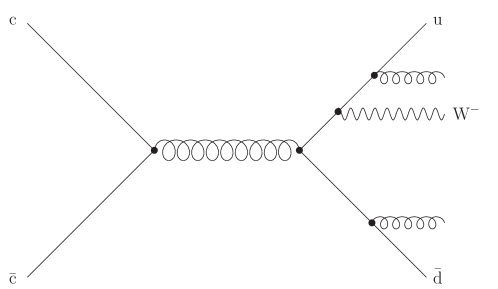
Figure 1: An example of a matrix element contribution without a complete shower history. If the parton shower does not include Wlimit-fromW\mathrm{W}-boson radiation, only the two gluon emissions can be reclustered, and cc¯ud¯Wc¯cu¯dsuperscriptW\mathrm{c}\bar{\mathrm{c}}\to\mathrm{u}\bar{\mathrm{d}}\mathrm{W}^{-} has to be considered a separate hard process.

A well-known challenge of merging prescriptions is the treatment of configurations that could never have been produced by a sequence of shower splittings. This can happen if the PS does not include all possible splittings of the model. Figure 1 for example cannot be produced by a shower that does not allow Wlimit-fromW\mathrm{W}-boson radiation. Such states cannot be projected onto a lower-multiplicity underlying process, and will thus introduce small unitarity violations in UMEPS.

4.1 Procedure step-by-step

To implement UMEPS, we need to be able to perform the necessary integrations. Although the formulae could convey a feeling of complexity, these integrations are factually already needed in traditional merging approaches. All modern CKKW-inspired schemes need to construct a history of parton shower states for input matrix element events, because otherwise, no trial showers can be used to generate Sudakov form factors dynamically. Thus, a sequence of states S+nS+n1S+1S+0subscript𝑆𝑛subscript𝑆𝑛1subscript𝑆1subscript𝑆0S_{+n}\rightarrow S_{+n-1}\rightarrow\dots\rightarrow S_{+1}\rightarrow S_{+0} is always available. The sequence is constructed by inverting the shower mapping of radiative phase space on each state, i.e. a parton in S+nsubscript𝑆𝑛S_{+n} is removed, and its momentum distributed amongst the remaining particles, leading to a state S+n1subscript𝑆𝑛1S_{+n-1}555 The mapping used for the current paper is given in Appendix B.2 of [16]. This is exactly the integration we need: To produce the integrated version of S+nsubscript𝑆𝑛S_{+n}, we simply replace it by S+n1subscript𝑆𝑛1S_{+n-1}, but keep the full weight. klimit-from𝑘k-fold integrations can be achieved by replacing S+nsubscript𝑆𝑛S_{+n} with S+nksubscript𝑆𝑛𝑘S_{+n-k}.

With this, we have all ingredients to construct the UMEPS scheme. If not mentioned explicitly, all weights in UMEPS are generated precisely as in CKKW-L. To avoid unnecessary complications, we will here gloss over many technicalities that have already been addressed in CKKW-L, and are directly borrowed by UMEPS. A discussion of Sudakov reweighting for states without parton-shower ordered histories, for example, can be found in [16].

The UMEPS algorithm has two parts – a part in which we keep the matrix element configurations (B^nlimit-fromsubscript^B𝑛\widehat{\textnormal{B}}_{n}-events) and another in which we integrate over emissions (sB^nmlimit-fromsubscript𝑠subscript^B𝑛𝑚\int_{s}\widehat{\textnormal{B}}_{n\rightarrow m}-events):

  1. I.

    Produce Les Houches event files (LHEF) [25] with a matrix element generator for n=0,1N𝑛01𝑁n~{}=~{}0,1\ldots N extra jets with a regularisation cut-off, ρMSsubscript𝜌MS\rho_{\textnormal{\tiny MS}}, typically using a fixed factorisation scale, μFsubscript𝜇𝐹\mu_{F}, and a fixed αs(μR)subscript𝛼ssubscript𝜇𝑅\alpha_{\mathrm{s}}(\mu_{R}).

  2. II.

    Pick a jet multiplicity, n𝑛n, and a state S+nsubscript𝑆𝑛S_{+n} according to the cross sections given by the matrix element generator.

    1. 1.

      Find all shower histories for the state S+nsubscript𝑆𝑛S_{+n}, pick a sequence according to the product of splitting probabilities. Only pick un-ordered sequences if no ordered sequence was found. Only pick incomplete paths if no complete path was constructed.

    2. 2.

      Perform reweighting: For each 0i<n0𝑖𝑛0\leqslant i<n,

      1. i.

        Start the shower off the state S+isubscript𝑆𝑖S_{+i} at ρisubscript𝜌𝑖\rho_{i}, generate a trial state R𝑅R with scale ρRsubscript𝜌𝑅\rho_{R}. If ρR>ρi+1subscript𝜌𝑅subscript𝜌𝑖1\rho_{R}>\rho_{i+1}, veto the event and start again from II.

      2. ii.

        Calculate the weight factor

        wi=αs(ρi+1)αs(μR)xi+fi+(xi+,ρi)xi+fi+(xi+,ρi+1)xifi(xi,ρi)xifi(xi,ρi+1)subscript𝑤𝑖subscript𝛼ssubscript𝜌𝑖1subscript𝛼ssubscript𝜇𝑅superscriptsubscript𝑥𝑖superscriptsubscript𝑓𝑖superscriptsubscript𝑥𝑖subscript𝜌𝑖superscriptsubscript𝑥𝑖superscriptsubscript𝑓𝑖superscriptsubscript𝑥𝑖subscript𝜌𝑖1superscriptsubscript𝑥𝑖superscriptsubscript𝑓𝑖superscriptsubscript𝑥𝑖subscript𝜌𝑖superscriptsubscript𝑥𝑖superscriptsubscript𝑓𝑖superscriptsubscript𝑥𝑖subscript𝜌𝑖1w_{i}=\frac{\alpha_{\mathrm{s}}(\rho_{i+1})}{\alpha_{\mathrm{s}}(\mu_{R})}\frac{x_{i}^{+}f_{i}^{+}(x_{i}^{+},\rho_{i})}{x_{i}^{+}f_{i}^{+}(x_{i}^{+},\rho_{i+1})}\frac{x_{i}^{-}f_{i}^{-}(x_{i}^{-},\rho_{i})}{x_{i}^{-}f_{i}^{-}(x_{i}^{-},\rho_{i+1})} (39)
    3. 3.

      Start the shower from S+nsubscript𝑆𝑛S_{+n}.

      1. i.

        If n<N𝑛𝑁n<N, start the shower at ρnsubscript𝜌𝑛\rho_{n}, veto any shower emission producing an additional resolved jet.

      2. ii.

        If n=N𝑛𝑁n=N, start the shower at ρnsubscript𝜌𝑛\rho_{n}.

  3. III.

    If the event was not rejected, multiply the event weight by

    wn=xn+fn+(xn+,ρn)xn+fn+(xn+,μF)×xnfn(xn,ρn)xnfn(xn,μF)×i=0n1wisuperscriptsubscript𝑤𝑛superscriptsubscript𝑥𝑛superscriptsubscript𝑓𝑛superscriptsubscript𝑥𝑛subscript𝜌𝑛superscriptsubscript𝑥𝑛superscriptsubscript𝑓𝑛superscriptsubscript𝑥𝑛subscript𝜇𝐹superscriptsubscript𝑥𝑛superscriptsubscript𝑓𝑛superscriptsubscript𝑥𝑛subscript𝜌𝑛superscriptsubscript𝑥𝑛superscriptsubscript𝑓𝑛superscriptsubscript𝑥𝑛subscript𝜇𝐹superscriptsubscriptproduct𝑖0𝑛1subscript𝑤𝑖w_{n}^{\prime}=\frac{x_{n}^{+}f_{n}^{+}(x_{n}^{+},\rho_{n})}{x_{n}^{+}f_{n}^{+}(x_{n}^{+},\mu_{F})}\times\frac{x_{n}^{-}f_{n}^{-}(x_{n}^{-},\rho_{n})}{x_{n}^{-}f_{n}^{-}(x_{n}^{-},\mu_{F})}\times\prod_{i=0}^{n-1}w_{i} (40)
  4. V.

    Start again from II.

The second part, i.e. producing sB^nmlimit-fromsubscript𝑠subscript^B𝑛𝑚\int_{s}\widehat{\textnormal{B}}_{n\rightarrow m}-events to effect lower-multiplicity PS resummation, requires only two changes:

  1. II.3

    Replace the matrix-element state by S+n1subscript𝑆𝑛1S_{+n-1}, or the first state S+lsubscript𝑆𝑙S_{+l} with all ln1𝑙𝑛1l\leq n-1 partons above the merging scale. If no integrated state can be constructed, i.e. if only incomplete paths were found, reject the event. For valid events, start the shower at ρnsubscript𝜌𝑛\rho_{n}, veto any shower emission producing an additional resolved jet.

  2. III.

    If the event was not rejected, multiply the event weight by

    wn=xn+fn+(xn+,ρn)xn+fn+(xn+,μF)×xnfn(xn,ρn)xnfn(xn,μF)×i=0n1wisuperscriptsubscript𝑤𝑛superscriptsubscript𝑥𝑛superscriptsubscript𝑓𝑛superscriptsubscript𝑥𝑛subscript𝜌𝑛superscriptsubscript𝑥𝑛superscriptsubscript𝑓𝑛superscriptsubscript𝑥𝑛subscript𝜇𝐹superscriptsubscript𝑥𝑛superscriptsubscript𝑓𝑛superscriptsubscript𝑥𝑛subscript𝜌𝑛superscriptsubscript𝑥𝑛superscriptsubscript𝑓𝑛superscriptsubscript𝑥𝑛subscript𝜇𝐹superscriptsubscriptproduct𝑖0𝑛1subscript𝑤𝑖-w_{n}^{\prime}=-\frac{x_{n}^{+}f_{n}^{+}(x_{n}^{+},\rho_{n})}{x_{n}^{+}f_{n}^{+}(x_{n}^{+},\mu_{F})}\times\frac{x_{n}^{-}f_{n}^{-}(x_{n}^{-},\rho_{n})}{x_{n}^{-}f_{n}^{-}(x_{n}^{-},\mu_{F})}\times\prod_{i=0}^{n-1}w_{i} (41)

Finally, all samples generated in the first and second parts are added to give the UMEPS prediction. Note that in order produce correctly normalised cross sections dσiexdϕ0𝑑superscriptsubscript𝜎𝑖𝑒𝑥𝑑subscriptitalic-ϕ0\frac{d\sigma_{i}^{ex}}{d\phi_{0}}, we need to include ratios of parton distributions and αssubscript𝛼s\alpha_{\mathrm{s}} ratios into the weight. This is analogous to the CKKW-L method (see the αssubscript𝛼s\alpha_{\mathrm{s}}- and PDF-factors in eq. (14)). It is worthwhile to notice that the UMEPS scheme can in principle be implemented by using structures already existing in traditional merging codes. Basically, compared to traditional merging, the B^nlimit-fromsubscript^B𝑛\widehat{\textnormal{B}}_{n}-contributions do not carry a no-emission probability for emissions off the ME event. The sB^nmlimit-fromsubscript𝑠subscript^B𝑛𝑚\int_{s}\widehat{\textnormal{B}}_{n\rightarrow m}-samples can easily be extracted from merging codes.

How multiple partonic interactions (MPI) are added to the merged samples requires a short discussion. In principle, we stay true to the philosophy of the algorithm outlined in [16], i.e. we want to make sure that the merging method does not artificially suppress hard secondary scatterings, which in PYTHIA8 are interleaved with the parton shower. The interleaving means that the PS is competing with the MPI’s, and the probability of emitting a parton in the PS is not only governed by the standard no-emission probability, ΠS+nsubscriptΠsubscript𝑆𝑛\Pi_{S_{+n}} but is also multiplied by a no-MPI probability, ΠS+nMPIsuperscriptsubscriptΠsubscript𝑆𝑛MPI\Pi_{S_{+n}}^{\mathrm{MPI}}. Hence all m𝑚m-jet (both B^msubscript^B𝑚\widehat{\textnormal{B}}_{m} and sB^nmsubscript𝑠subscript^B𝑛𝑚\int_{s}\widehat{\textnormal{B}}_{n\rightarrow m}) samples generated by our algorithm above need to be multiplied by the no-MPI probabilities

i=0m1ΠS+iMPI(ρi,ρi+1),superscriptsubscriptproduct𝑖0𝑚1superscriptsubscriptΠsubscript𝑆𝑖MPIsubscript𝜌𝑖subscript𝜌𝑖1\prod_{i=0}^{m-1}\Pi_{S_{+i}}^{\mathrm{MPI}}(\rho_{i},\rho_{i+1}), (42)

which are easily incorporated in the trial showers described above. We also need to include the actual MPI’s. Here the philosophy is that as soon as we have a MPI at some scale, we ignore corrections from the full tree-level matrix element on softer jets from the primary interaction, and allow them to be described by the PS alone. Hence, when we start the shower from a given m𝑚m-parton state (with m<N𝑚𝑁m<N) in step II.3, we choose the reconstructed ρmsubscript𝜌𝑚\rho_{m} as starting scale. As described before, we veto any parton emission above ρMSsubscript𝜌MS\rho_{\textnormal{\tiny MS}}. However, if a MPI is generated above ρMSsubscript𝜌MS\rho_{\textnormal{\tiny MS}}, it is accepted and the shower is allowed to continue without any further veto. (For the m=N𝑚𝑁m=N case, the shower including MPI is allowed without restrictions, starting from ρNsubscript𝜌𝑁\rho_{N}.) In this way we achieve the same goal as in [16]: If the nN𝑛𝑁n\leq N hardest jets in an event all belong to the primary interaction, they are described by the tree-level ME, while all other jets are given by the (interleaved) PS. Just as in [16], the treatment of pure QCD jet production means that the Born-level cross section is properly eikonalized by the no-MPI factor, by allowing MPI’s all the way from s𝑠\sqrt{s} in the trial shower for ΠS+0MPIsuperscriptsubscriptΠsubscript𝑆0MPI\Pi_{S_{+0}}^{\mathrm{MPI}}.

5 Results

We have implemented UMEPS merging in PYTHIA8, and will make the necessary code public in the next major release version. In this section, we will concentrate on predictions for WW\mathrm{W}-boson and QCD jet production at the LHC. However, the code aims to achieve the same generality as the implementation of CKKW-L in PYTHIA8.

All input matrix element configurations are taken from Les Houches Event Files generated with MadGraph/MadEvent, with the following settings:

  • Fixed renormalisation scale μR=MZ2subscript𝜇𝑅superscriptsubscriptMZ2\mu_{R}=\textnormal{M}_{\textnormal{\tiny{Z}}}^{2}, fixed factorisation scale μF=MW2subscript𝜇𝐹superscriptsubscriptMW2\mu_{F}=\textnormal{M}_{\textnormal{\tiny{W}}}^{2} for WW\mathrm{W}-production. For 22222\to 2 processes in pure QCD, we use μr,22=m,1m,1subscript𝜇𝑟22subscript𝑚perpendicular-to1subscript𝑚perpendicular-to1\mu_{r,2\to 2}=m_{\perp,1}m_{\perp,1} and μf,22=min{m,12,m,12}subscript𝜇𝑓22subscriptsuperscript𝑚2perpendicular-to1subscriptsuperscript𝑚2perpendicular-to1\mu_{f,2\to 2}=\min\{m^{2}_{\perp,1},m^{2}_{\perp,1}\}.

  • CTEQ6L1 parton distributions and αs(MZ2)=0.130subscript𝛼ssuperscriptsubscriptMZ20.130\alpha_{\mathrm{s}}(\textnormal{M}_{\textnormal{\tiny{Z}}}^{2})=0.130.

  • The merging scale ρMSsubscript𝜌MS\rho_{\textnormal{\tiny MS}} is defined by the minimal PYTHIA8 evolution p,ijksubscript𝑝perpendicular-to𝑖𝑗𝑘p_{\perp,ijk} of all possible combinations of three partons in the event. p,ijksubscript𝑝perpendicular-to𝑖𝑗𝑘p_{\perp,ijk} for a single combination of three particles i𝑖i, j𝑗j and k𝑘k is defined as

    p,ijk2={zijk(1zijk)Qij2withQij2=(pi+pj)2,zijk=xi,jkxi,jk+xj,ik,xi,jk=2pi(pi+pj+pk)(pi+pj+pk)2for FSR(1zijk)Qij2withQij2=(pipj)2,zijk=(pipj+pk)2(pi+pk)2for ISRsubscriptsuperscript𝑝2perpendicular-to𝑖𝑗𝑘casessubscript𝑧𝑖𝑗𝑘1subscript𝑧𝑖𝑗𝑘superscriptsubscript𝑄𝑖𝑗2withsuperscriptsubscript𝑄𝑖𝑗2superscriptsubscript𝑝𝑖subscript𝑝𝑗2,subscript𝑧𝑖𝑗𝑘subscript𝑥𝑖𝑗𝑘subscript𝑥𝑖𝑗𝑘subscript𝑥𝑗𝑖𝑘,otherwisesubscript𝑥𝑖𝑗𝑘2subscript𝑝𝑖subscript𝑝𝑖subscript𝑝𝑗subscript𝑝𝑘superscriptsubscript𝑝𝑖subscript𝑝𝑗subscript𝑝𝑘2for FSR1subscript𝑧𝑖𝑗𝑘superscriptsubscript𝑄𝑖𝑗2withsuperscriptsubscript𝑄𝑖𝑗2superscriptsubscript𝑝𝑖subscript𝑝𝑗2,subscript𝑧𝑖𝑗𝑘superscriptsubscript𝑝𝑖subscript𝑝𝑗subscript𝑝𝑘2superscriptsubscript𝑝𝑖subscript𝑝𝑘2otherwisefor ISR\displaystyle p^{2}_{\perp,ijk}=\begin{cases}z_{ijk}(1-z_{ijk})Q_{ij}^{2}&~{}\textnormal{with}~{}Q_{ij}^{2}=(p_{i}+p_{j})^{2}~{}\textnormal{,}~{}z_{ijk}=\frac{x_{i,jk}}{x_{i,jk}+x_{j,ik}}~{}\textnormal{,}{}\\ &x_{i,jk}=\frac{2p_{i}(p_{i}+p_{j}+p_{k})}{(p_{i}+p_{j}+p_{k})^{2}}\quad\textnormal{for FSR}\\ (1-z_{ijk})Q_{ij}^{2}&~{}\textnormal{with}~{}Q_{ij}^{2}=-(p_{i}-p_{j})^{2}~{}\textnormal{,}~{}z_{ijk}=\frac{(p_{i}-p_{j}+p_{k})^{2}}{(p_{i}+p_{k})^{2}}\\ &\textnormal{for ISR}\end{cases} (43)
  • In QCD 22222\to 2 scatterings, the kinematical transverse momentum of jets is required to be larger than pT,j=5subscript𝑝𝑇𝑗5p_{T,j}=5 GeV.

The value of αs(MZ2)subscript𝛼ssuperscriptsubscriptMZ2\alpha_{\mathrm{s}}(\textnormal{M}_{\textnormal{\tiny{Z}}}^{2}) was set to match the αssubscript𝛼s\alpha_{\mathrm{s}}-value obtained in fitting the PDFs used in the ME calculation. To generate results, we have chosen the merging scale definition to closely match the parton shower evolution variable. The algorithm does however not depend on this particular choice. All jets needed for analysis purposes were defined with help of fastjet-routines [26]. The momentum of the intermediate WW\mathrm{W}-boson will, if required, be extracted directly from the Monte Carlo event. We will compare UMEPS to the CKKW-L implementation in PYTHIA8. The problems we choose to highlight should be regarded as criticism of the implementation in PYTHIA8, rather than an assessment of CKKW-inspired methods in general.

5.1 W-boson production
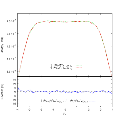
Refer to caption
Refer to caption
Figure 2: Comparison between 𝒪(αs)𝒪subscript𝛼s\mathcal{O}(\alpha_{\mathrm{s}})-terms of the parton shower with integrated matrix elements, for WW\mathrm{W}-boson production in pppp\mathrm{p}\mathrm{p} collisions at ECM=7000subscript𝐸CM7000E_{\mathrm{CM}}=7000 GeV. The merging scale value is ρMS=15subscript𝜌MS15\rho_{\textnormal{\tiny MS}}=15 GeV. Left panel: Rapidity of the WW\mathrm{W}-boson, intended for comparison between the integrated one-jet matrix element (labelled [dσ10/dyw]𝒪(αs1)subscriptdelimited-[]𝑑subscript𝜎10𝑑subscript𝑦𝑤𝒪superscriptsubscript𝛼s1\left[d\sigma_{1\rightarrow 0}/dy_{w}\right]_{\mathcal{O}(\alpha_{\mathrm{s}}^{1})} ​) and the 𝒪(αs1)𝒪superscriptsubscript𝛼s1\mathcal{O}(\alpha_{\mathrm{s}}^{1})-term of the no-emission probability for having no emission above ρMSsubscript𝜌MS\rho_{\textnormal{\tiny MS}} radiated off zero-jet states above ρMSsubscript𝜌MS\rho_{\textnormal{\tiny MS}} (labelled [dσ0/dyw]𝒪(αs1)subscriptdelimited-[]𝑑subscript𝜎0𝑑subscript𝑦𝑤𝒪superscriptsubscript𝛼s1\left[d\sigma_{0}/dy_{w}\right]_{\mathcal{O}(\alpha_{\mathrm{s}}^{1})} ​). Right panel: Transverse momentum of the parton, for W+jW𝑗\mathrm{W}+j production in pppp\mathrm{p}\mathrm{p} collisions at ECM=7000subscript𝐸CM7000E_{\mathrm{CM}}=7000 GeV, intended for comparison between the integrated two-jet matrix element (labelled [dσ21/dp]𝒪(αs2)subscriptdelimited-[]𝑑subscript𝜎21𝑑subscript𝑝perpendicular-to𝒪superscriptsubscript𝛼s2\left[d\sigma_{2\rightarrow 1}/dp_{\perp}\right]_{\mathcal{O}(\alpha_{\mathrm{s}}^{2})} ​) and the 𝒪(αs1)𝒪superscriptsubscript𝛼s1\mathcal{O}(\alpha_{\mathrm{s}}^{1})-term of the no-emission probability for having no emission above ρMSsubscript𝜌MS\rho_{\textnormal{\tiny MS}} radiated off one-jet states, multiplying the W+jW𝑗\mathrm{W}+j matrix element (labelled [dσ1/dp]𝒪(αs2)subscriptdelimited-[]𝑑subscript𝜎1𝑑subscript𝑝perpendicular-to𝒪superscriptsubscript𝛼s2\left[d\sigma_{1}/dp_{\perp}\right]_{\mathcal{O}(\alpha_{\mathrm{s}}^{2})} ​).

We begin by comparing the result of the removal of a jet by integration with the corresponding parton shower contribution. This is useful to assess if performing the integration by the replacement S+n+1S+nsubscript𝑆𝑛1subscript𝑆𝑛S_{+n+1}\rightarrow S_{+n} produces the desired results.

In the left panel of Figure 2, we compare the integrated one-jet matrix element (i.e. the 𝒪(αs1(μR))𝒪superscriptsubscript𝛼s1subscript𝜇𝑅\mathcal{O}\left(\alpha_{\mathrm{s}}^{1}\left(\mu_{R}\right)\right)-term of eq. (32)) with the shower approximation of the 𝒪(αs1(μR))𝒪superscriptsubscript𝛼s1subscript𝜇𝑅\mathcal{O}\left(\alpha_{\mathrm{s}}^{1}\left(\mu_{R}\right)\right)-term in zero-jet events. The second term is of course just the 𝒪(αs1(μR))𝒪superscriptsubscript𝛼s1subscript𝜇𝑅\mathcal{O}\left(\alpha_{\mathrm{s}}^{1}\left(\mu_{R}\right)\right)-contribution in eq. (18). The rapidity of the WW\mathrm{W}-boson is identical in these two samples because PYTHIA8 is already matrix-element corrected for W+jW𝑗\mathrm{W}+j-states. This demonstrates that in WW\mathrm{W}-boson production, generating the no-emission probability in zero-jet states with PYTHIA8, or by a reweighted, integrated one-jet matrix element are both legitimate ways to produce the same factor.

The right panel of Figure 2 investigates the difference between the parton shower approximation of no resolved emissions in one-jet states between the scales ρ1subscript𝜌1\rho_{1} and ρMSsubscript𝜌MS\rho_{\textnormal{\tiny MS}} and the result of constructing an unresolved emission by integrating over one parton in a two-jet matrix element. This means that we compare the one-jet matrix element, multiplied by the 𝒪(αs1(μR))𝒪superscriptsubscript𝛼s1subscript𝜇𝑅\mathcal{O}\left(\alpha_{\mathrm{s}}^{1}\left(\mu_{R}\right)\right)-term of the no-emission probability ΠS+1(x1,ρ1,ρMS)subscriptΠsubscript𝑆1subscript𝑥1subscript𝜌1subscript𝜌MS\Pi_{S_{+1}}(x_{1},\rho_{1},\rho_{\textnormal{\tiny MS}}) in eq. (3), with the 𝒪(αs2(μR))𝒪superscriptsubscript𝛼s2subscript𝜇𝑅\mathcal{O}\left(\alpha_{\mathrm{s}}^{2}\left(\mu_{R}\right)\right)-contribution in eq. (34). The comparison shows that, as expected, the parton shower underestimates the hardness of the unresolved (second) emission, which is reminiscent of the fact that the inclusion of two-jet matrix elements into the PS prediction does in general increase the tail of the psubscript𝑝perpendicular-top_{\perp} of the hardest jet.

Refer to caption
Refer to caption
Figure 3: Transverse momentum of the hardest jet, for WW\mathrm{W}-boson production in pppp\mathrm{p}\mathrm{p} collisions at ECM=7000subscript𝐸CM7000E_{\mathrm{CM}}=7000 GeV, when merging up to two additional partons. Jets were defined with the ksubscript𝑘perpendicular-tok_{\perp}-algorithm, with k,min=10subscript𝑘perpendicular-to𝑚𝑖𝑛10k_{\perp,min}=10 GeV. Multi-parton interactions and hadronisation were excluded. Left panel: Results of the CKKW-L scheme. The contributions are labelled Bw00subscriptsubscript𝑤00{}_{0}w_{0}, Bw11subscriptsubscript𝑤11{}_{1}w_{1} and Bw22subscriptsubscript𝑤22{}_{2}w_{2} for CKKW-L-reweighted zero-, one- and two-jet matrix elements, respectively. Right panel: Results of the UMEPS scheme. The contributions are labelled B^0subscript^B0\widehat{\textnormal{B}}_{0}, B^1subscript^B1\widehat{\textnormal{B}}_{1} and B^2subscript^B2\widehat{\textnormal{B}}_{2} for UMEPS-reweighted zero-, one- and two-jet matrix elements, and sB^10subscript𝑠subscript^B10\int_{s}\widehat{\textnormal{B}}_{1\rightarrow 0} and sB^21subscript𝑠subscript^B21\int_{s}\widehat{\textnormal{B}}_{2\rightarrow 1} for UMEPS-reweighted, integrated one- and two-jet samples. sB^20subscript𝑠subscript^B20\int_{s}\widehat{\textnormal{B}}_{2\rightarrow 0} indicates the two-jet contribution that was integrated twice because the state S+1subscript𝑆1S_{+1} after the first integration contained an unresolved jet.

In Figure, 3 we show how matrix element samples contribute to this increase. All jet multiplicities enter, because the merging scale is not defined as the jet-separation of the ksubscript𝑘perpendicular-tok_{\perp}-algorithm, and since the merging scale cut acts on the matrix element state, while the jets are constructed from outgoing particles after the parton shower cascade. In CKKW-L, the high-psubscript𝑝perpendicular-top_{\perp} tail is dominated by the two-jet matrix element, with a major contribution from the one-jet states. The latter is significantly lower in UMEPS, a fact that we think crucial. UMEPS correctly cancels the inclusion of phase space points with two resolved jets by using the two-jet matrix element to construct a better approximation of radiating an unresolved parton from one-jet states. We see both in CKKW-L (left panel of Figure 3), and in Figure 2, that the parton shower underestimates the hardness of two-parton states. The description of unresolved emissions enters into the no-emission probabilities, with a negative 𝒪(αs1)𝒪superscriptsubscript𝛼s1\mathcal{O}(\alpha_{\mathrm{s}}^{1})-term. Thus, the contribution of showered one-jet states to the tail of p1subscript𝑝perpendicular-toabsent1p_{\perp 1} will be larger if the shower description of two-jet states underestimates hardness. UMEPS improves the description of the no-emission probability by ensuring that in inclusive observables, resolved two-jet states are cancelled, a feature that is at work in the tail of p1subscript𝑝perpendicular-toabsent1p_{\perp 1}.

Refer to caption
Refer to caption
Figure 4: Transverse momentum of the hardest jet, for WW\mathrm{W}-boson production in pppp\mathrm{p}\mathrm{p} collisions at ECM=7000subscript𝐸CM7000E_{\mathrm{CM}}=7000 GeV, when merging up to two additional partons. Jets were defined with the ksubscript𝑘perpendicular-tok_{\perp}-algorithm, with k,min=10subscript𝑘perpendicular-to𝑚𝑖𝑛10k_{\perp,min}=10 GeV. Multi-parton interactions and hadronisation were excluded. The lower insets show the deviation of merged results from default PYTHIA8, for three different ρMSsubscript𝜌MS\rho_{\textnormal{\tiny MS}}-values. Left panel: Results of the CKKW-L scheme. Right panel: Results of the UMEPS scheme.

Variations in the description of p1subscript𝑝perpendicular-toabsent1p_{\perp 1} are also visible in Figure 4, where we show the transverse momentum of the hardest jet in CKKW-L and UMEPS666Note that the co-variation of merged results in the ratio inset is due to fluctuations in the PYTHIA8 reference curve.. The trend sketched in the previous paragraph is particularly clear in the insets comparing to default PYTHIA8: UMEPS produces a softer tail in p1subscript𝑝perpendicular-toabsent1p_{\perp 1} than CKKW-L. The harder tail in CKKW-L is due to a worse description of unresolved emissions. It is fair to say that the difference between CKKW-L and UMEPS hints at the size of relic effects from not cancelling the higher-multiplicity matrix elements in a well-defined way. Merging scale variations in tree-level merging schemes arise from a mismatch of unresolved emissions exponentiated in no-emission probabilities and tree-level matrix elements for hard, resolved jets. UMEPS has a significantly lower merging scale variation since the method enforces a cancellation of resolved and unresolved contributions.
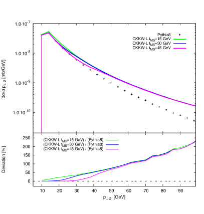
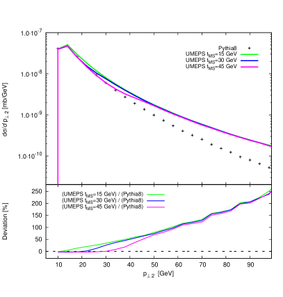
Refer to caption
Refer to caption
Figure 5: Transverse momentum of the second-hardest jet, for WW\mathrm{W}-boson production in pppp\mathrm{p}\mathrm{p} collisions at ECM=7000subscript𝐸CM7000E_{\mathrm{CM}}=7000 GeV. Jets were defined with the ksubscript𝑘perpendicular-tok_{\perp}-algorithm, with k,min=10subscript𝑘perpendicular-to𝑚𝑖𝑛10k_{\perp,min}=10 GeV, when merging up to two additional partons. Multi-parton interactions and hadronisation were excluded. The lower insets show the deviation of merged results from default PYTHIA8, for three different ρMSsubscript𝜌MS\rho_{\textnormal{\tiny MS}}-values. Left panel: Results of the CKKW-L scheme. Right panel: Results of the UMEPS scheme.

Figure 5 shows that for very exclusive observables, CKKW-L and UMEPS are virtually indistinguishable. In this example, this is of course expected since the treatment of the highest multiplicity (here, the two-jet) matrix element is identical for both cases.
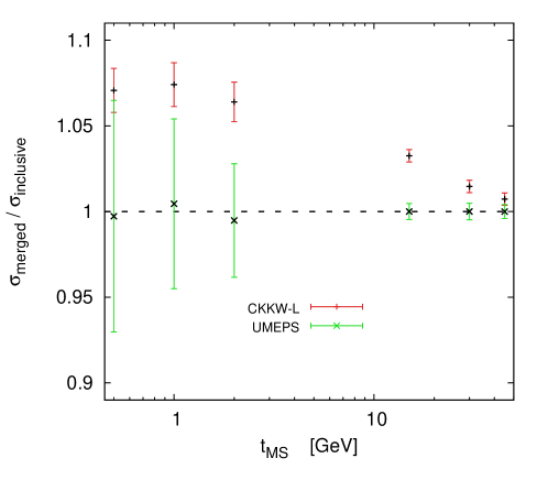
Refer to caption
Figure 6: Inclusive cross section for UMEPS- and CKKW-L merging of up to two additional jets in WW\mathrm{W}-boson production in pppp\mathrm{p}\mathrm{p} collisions at ECM=7000subscript𝐸CM7000E_{\mathrm{CM}}=7000 GeV (labelled σmergedsubscript𝜎merged\sigma_{\textnormal{merged}}), in comparison to the the lowest-multiplicity inclusive cross section σinclusivesubscript𝜎inclusive\sigma_{\textnormal{inclusive}}. The error bars represent only the statistical error on the merged cross section. For the UMEPS sample this becomes large for small merging scales, but as it is the same samples which are added and the subtracted, the central value stays very close to unity.

We would now like to perform a stress-test of the merging scale dependence. Since UMEPS properly cancels the effects of adding multi-jet matrix elements by subtracting their integrated counter-parts, it is in principle possible to push the merging scale to very small values. The variation of the inclusive cross section is shown in Figure 6. It is clear that UMEPS does indeed preserve the inclusive cross section, while for CKKW-L, very small merging scales lead to large changes, rendering the method unreliable. However, the error convergence in UMEPS is, due to the negative weights, significantly slower. We will comment on this below.
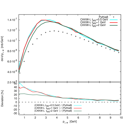
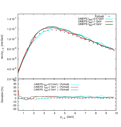
Refer to caption
Refer to caption
Figure 7: Transverse momentum of the WW\mathrm{W}-boson, for WW\mathrm{W}-boson production in pppp\mathrm{p}\mathrm{p} collisions at ECM=7000subscript𝐸CM7000E_{\mathrm{CM}}=7000 GeV, when merging up to two additional partons. Multi-parton interactions and hadronisation were excluded. The PYTHIA8 results are generated with the default settings, in particular with a primordial transverse momentum of k,p=2subscript𝑘perpendicular-to𝑝2k_{\perp,p}=2 GeV. All merged curves have been generated with k,p=0.5subscript𝑘perpendicular-to𝑝0.5k_{\perp,p}=0.5 GeV. The lower insets show the deviation of merged results from default PYTHIA8, for three different ρMSsubscript𝜌MS\rho_{\textnormal{\tiny MS}}-values. Left panel: Results of the CKKW-L scheme. Right panel: Results of the UMEPS scheme.

These unitarity violations might not induce drastic effects in the description of hard-scale observables like the transverse-momentum distribution of the WW\mathrm{W}-boson. However, magnifying the low-scale description of this observable (Figure 7) reveals problems. Figure 7 serves two purposes. It clearly shows that by pushing the merging scale to small values in CKKW-L, sub-leading contributions in the multi-jet matrix elements start to contribute more. Since those sub-leading contributions cannot be cancelled by the default parton shower, major increases over PYTHIA8 are found. UMEPS explicitly cancels these sub-leading terms, and thus leads to a reliable prediction. The second observation in Figure 7 is the dependence on the primordial transverse momentum parameter k,psubscript𝑘perpendicular-to𝑝k_{\perp,p}. This parameter was introduced in event generators to account for the transverse momentum of partons in the incoming protons, which cannot be generated in initial state DGLAP evolution. If this were the only effect to be modelled by k,psubscript𝑘perpendicular-to𝑝k_{\perp,p}, a value of k,p0.3subscript𝑘perpendicular-to𝑝0.3k_{\perp,p}\approx 0.3 GeV per incoming parton would seem appropriate. However, in current event generator tunes, significantly higher values (k,p2subscript𝑘perpendicular-to𝑝2k_{\perp,p}\approx 2 GeV) are required [20, 27], potentially to compensate for an incomplete phase space coverage in initial state showers due to the shower cut-off. The value of k,psubscript𝑘perpendicular-to𝑝k_{\perp,p} is mainly fixed by tuning to the position of the peak of the transverse momentum spectrum of the ZZ\mathrm{Z}- or WW\mathrm{W} boson. Increasing the value of k,psubscript𝑘perpendicular-to𝑝k_{\perp,p} roughly corresponds to pushing the peak to higher psubscript𝑝perpendicular-top_{\perp} values. Figure 7 compares the UMEPS and CKKW-L predictions for the transverse momentum of the WW\mathrm{W} boson, with k,p=0.5subscript𝑘perpendicular-to𝑝0.5k_{\perp,p}=0.5 GeV, to default, tuned PYTHIA8 with k,p=2.0subscript𝑘perpendicular-to𝑝2.0k_{\perp,p}=2.0 GeV. Unitarity violations in CKKW-L pull the peak back to lower psubscript𝑝perpendicular-top_{\perp}. This fact is virtually unchanged if we had used k,p=2.0subscript𝑘perpendicular-to𝑝2.0k_{\perp,p}=2.0 for CKKW-L predictions instead, suggesting that if we positively wanted to use a very low merging scale, an increase in k,psubscript𝑘perpendicular-to𝑝k_{\perp,p} would be necessary. UMEPS on the other hand can be used with very low merging scales, and in particular shows the interesting feature of matching the default PYTHIA8 curve without having a high k,psubscript𝑘perpendicular-to𝑝k_{\perp,p} value. We believe this is due to a better modelling of logarithms of the form ln(1/x)1𝑥\ln\left(1/x\right), which are present in the matrix element, and which are included in a unitary way in UMEPS – allowing for a much more natural value of k,psubscript𝑘perpendicular-to𝑝k_{\perp,p}. This result is of course very preliminary, since there are e.g. correlations of the shower cut-off pminsubscript𝑝perpendicular-toabsentp_{\perp\min} and k,psubscript𝑘perpendicular-to𝑝k_{\perp,p}. One would hope that matrix-element merging would allow to lower pminsubscript𝑝perpendicular-toabsentp_{\perp\min}, which might mean having to make a compromise for the value of k,psubscript𝑘perpendicular-to𝑝k_{\perp,p}. We will come back to these aspects when presenting tunes for matrix-element-merged PYTHIA8 in a future publication.

5.2 Dijet production

We would further like to mention QCD dijet production at the LHC, since potential merging scale dependencies enter already when merging dijet- and three-jet matrix elements, and to demonstrate the flexibility of our implementation. The main objective of including QCD dijet production in this publication was to assess the treatment of MPI discussed at the end of section 4.1. This is most effectively done by comparing to data, and before these we would like to only stress one issue.
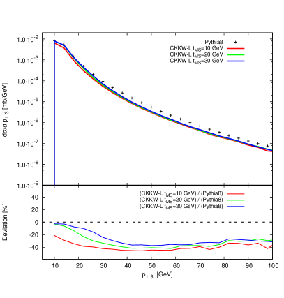
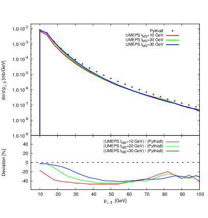
Refer to caption
Refer to caption
Figure 8: Transverse momentum of the third hardest jet, for pure QCD dijet production in pppp\mathrm{p}\mathrm{p} collisions at ECM=7000subscript𝐸CM7000E_{\mathrm{CM}}=7000 GeV, when merging up to two additional partons. Jets were defined with the ksubscript𝑘perpendicular-tok_{\perp}-algorithm, with k,min=10subscript𝑘perpendicular-to𝑚𝑖𝑛10k_{\perp,min}=10 GeV. Multi-parton interactions and hadronisation were excluded. The lower insets show the deviation of merged results from default PYTHIA8, for three different ρMSsubscript𝜌MS\rho_{\textnormal{\tiny MS}}-values. Left panel: Results of the CKKW-L scheme. Right panel: Results of the UMEPS scheme.

Figure 8 shows the transverse momentum of the third-hardest jet. We see that UMEPS and CKKW-L show very similar changes when compared to PYTHIA8. However, neither curves show the high-psubscript𝑝perpendicular-top_{\perp} increase seen in [16]. This is simply because we have revised the choice of the renormalisation scale in the core 22222\to 2 QCD scattering. In [16], the two powers of αs(μR)subscript𝛼ssubscript𝜇𝑅\alpha_{\mathrm{s}}(\mu_{R}) in the core 22222\to 2 process were never touched, and thus were evaluated with the rather unfortunate choice μR=MZ2subscript𝜇𝑅superscriptsubscriptMZ2\mu_{R}=\textnormal{M}_{\textnormal{\tiny{Z}}}^{2} in the input Les Houches events. This has been rectified in the current release of (CKKW-L in) PYTHIA8, i.e. the scale choice (μr,22=m,1m,1subscript𝜇𝑟22subscript𝑚perpendicular-to1subscript𝑚perpendicular-to1\mu_{r,2\to 2}=m_{\perp,1}m_{\perp,1}) is now dynamical. Potential reweighting (due to the usage of fixed μRsubscript𝜇𝑅\mu_{R} in the LHEF generation is handled internally in PYTHIA8. The trend that pure QCD multi-jet matrix elements have a softer spectrum of well-separated jets has already been observed in [16, 28]. The merging scale variation in UMEPS is within the statistical error of the samples. The statical uncertainty is larger in UMEPS than in CKKW-L, due to cancellations between positive and negative weights (see the last part on section 6).

5.3 Comparison with data

In this section, we would like to confront UMEPS with experimental data. Event generator predictions were obtained with the settings of Tune A2 [29]. The results should of course not be regarded as final statement, since changes in the perturbative physics in event generators in principle request a full re-tuning. The intention of this section is to investigate if after including matrix-element information, hard-scale features are closer to measurements, and to assess the changes in underlying event description. All plots were produced with RIVET [30]. We apologise if the selection of experimental measurements seems biased.
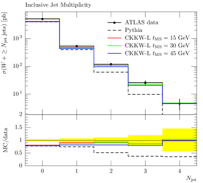
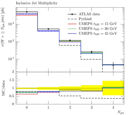
Refer to caption
Refer to caption
Figure 9: Jet multiplicity in WW\mathrm{W}-boson production, for three different merging scales, as measured by ATLAS [31]. Effects of multiple scatterings and hadronisation are included.

In Figure 9, we show jet rates in WW\mathrm{W}-boson production at the ATLAS [31]. We find an improved description after including up to two additional jets, and little differences between UMEPS and CKKW-L.
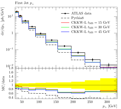
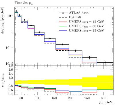
Refer to caption
Refer to caption
Figure 10: Transverse momentum of the hardest jet in WW\mathrm{W}-boson production, for three different merging scales, as measured by ATLAS [31]. Effects of multiple scatterings and hadronisation are included.

The transverse momentum of the hardest jet is shown in Figure 10. Again, we find that the shape description is improved by the CKKW-L and UMEPS methods. CKKW-L shows merging scale variations at lower psubscript𝑝perpendicular-top_{\perp}-values, since a slightly different inclusive cross section for a low merging scale leads to a slightly different normalisations. UMEPS on the other hand suffers from statistical fluctuations for a low merging scale value (ρMS=15subscript𝜌MS15\rho_{\textnormal{\tiny MS}}=15 GeV), while the curves for ρMS=30subscript𝜌MS30\rho_{\textnormal{\tiny MS}}=30 GeV and ρMS=45subscript𝜌MS45\rho_{\textnormal{\tiny MS}}=45 completely overlap. Note that the psubscript𝑝perpendicular-top_{\perp} spectrum of UMEPS is a little softer than CKKW-L, in accordance with Figure 4.
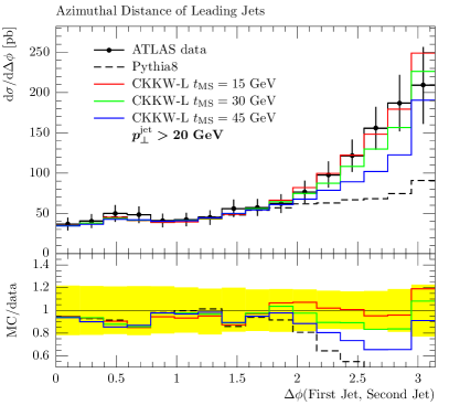
Refer to caption
Refer to caption
Figure 11: Azimuthal distance between the two hardest jets in WW\mathrm{W}-boson production, for three different merging scales, as measured by ATLAS [31]. Effects of multiple scatterings and hadronisation are included.

It is interesting to investigate when tree-level matrix element merging schemes produce large uncertainties. Figure 11 shows the azimuthal distance Δϕ12Δsubscriptitalic-ϕ12\Delta\phi_{12} between the two hardest jets. The parton shower alone cannot describe the peak at π𝜋\pi. If the merging scale is low, the two-jet matrix element will give the dominant contribution in the peak region. High merging scales will increase the influence of the shower, thus degrading the description of the peak. Thus, this observable carries major merging scale variations, and provides excellent guidance for future improvements.
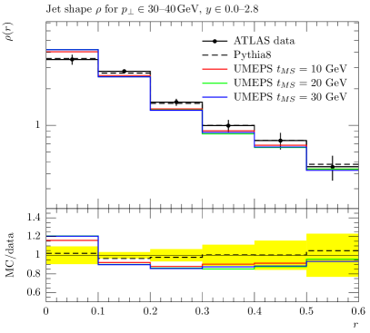
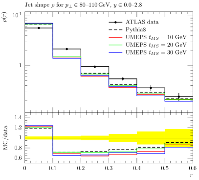
Refer to caption
Refer to caption
Figure 12: Jet shapes in QCD events, for three different merging scales, in two psubscript𝑝perpendicular-top_{\perp} bins, as measured by ATLAS [32]. Effects of multiple scatterings and hadronisation are included.
Refer to caption
Refer to caption
Figure 13: Sum of transverse momenta of charged particles in QCD events, for three different merging scales, in the transverse and toward region, as measured by ATLAS [33]. Effects of multiple scatterings and hadronisation are included.

Before moving to the discussion section, we would like to investigate how jet shapes at the LHC are changed by the inclusion of additional matrix elements in the pure QCD case. The ATLAS analysis [32] found that the differential jet shape for relatively low-psubscript𝑝perpendicular-top_{\perp} jets with p160subscript𝑝perpendicular-to160p_{\perp}\leq 160 GeV depends crucially on the modelling of the underlying event. In Figure 12, we show the default PYTHIA8 and UMEPS results for two psubscript𝑝perpendicular-top_{\perp} bins. Although far from perfect, the difference between the pure shower and merged results are similar to what a minor change in αssubscript𝛼s\alpha_{\mathrm{s}} would give777This of course does not mean that we will to use this data for tuning, but that αssubscript𝛼s\alpha_{\mathrm{s}}-choices for different tunes can have a comparable effect on ρ(r)𝜌𝑟\rho(r).. We are confident that the prescription for adding MPI (see section 4.1) does indeed mean that the underlying-event modelling of PYTHIA8 is only marginally perturbed by the inclusion of additional jets. This is supported by Figure 13, which shows the sum of charged-particle transverse momenta in region close to the leading track (i.e. the toward region) and perpendicular to the leading track (transverse region) [33]. These are typical minimum-bias observables especially designed to investigate the underlying event, and PYTHIA8 tune A2 includes this data in the tuning procedure. It is reassuring that the inclusion of two additional jets through the UMEPS scheme did not invalidate this tuning.

6 Discussion

Before concluding this letter, we would like to make some comments to put this method into perspective.

Relation to LoopSim

Even though not completely obvious at first sight, UMEPS was heavily influenced by the LoopSim method [34]. This method as introduced to tame order-by-order large logarithmic enhancements by combining matrix elements with different jet multiplicities in a unitary way. The combination is done by joining all combinations to integrate over 1,,n1𝑛1,\dots,n partons in the ME event S+nsubscript𝑆𝑛S_{+n}, and also allowing an integration over hard process particles. In figure 1, the final state gluons are candidates for integration (or, in the terminology of LoopSim, looping), and the Wlimit-fromW\mathrm{W}-boson can be looped as well. With such a procedure, enhancements due to collinear Wlimit-fromW\mathrm{W}-boson radiation off a dijet state can be compensated888At very large transverse momenta, the effect of multiple soft/collinear electroweak bosons becomes important. An appraisal of high-psubscript𝑝perpendicular-top_{\perp} observables in WZWZ\mathrm{W}\mathrm{Z}-production has recently been reported [35]..

Apart from major technical differences, one interesting difference is that in the LoopSim method, higher fixed-order corrections are approximated by multiple loopings, whereas in UMEPS, an all-order expression is included in the S+n+1subscript𝑆𝑛1S_{+n+1} state before one parton is looped. Integrating multiple emissions is only necessary for ρMSlimit-fromsubscript𝜌MS\rho_{\textnormal{\tiny MS}}-unordered sequences of splittings, which are not considered in LoopSim. Furthermore, in UMEPS, only integrations of QCD splittings are performed, while LoopSim includes loopings of Wlimit-fromW\mathrm{W}-boson radiation. We postpone the inclusion Wlimit-fromW\mathrm{W}-boson clusterings in UMEPS until a full electroweak shower is available in PYTHIA8. It would clearly be interesting to combine the Sudakov resummation in UMEPS with the multiple loopings done in LoopSim. To arrive at a better description of S+0subscript𝑆0S_{+0} configurations, one could e.g. take αs1superscriptsubscript𝛼s1\alpha_{\mathrm{s}}^{1} contributions from the looped S+1subscript𝑆1S_{+1} state, αs2superscriptsubscript𝛼s2\alpha_{\mathrm{s}}^{2} contributions from the twice-looped S+2subscript𝑆2S_{+2}, and all higher orders from Sudakov-reweighted thrice-integrated S+3subscript𝑆3S_{+3} events. The way the inclusive cross section is maintained in such a procedure will be less obvious than in the case of LoopSim or UMEPS.

Merging scale dependence

In the original CKKW-L algorithm it is evident that the dependence on the merging scale is absent to the accuracy of the PS. This means that for any observable, leading logarithmic terms on the form αsnL2nsuperscriptsubscript𝛼s𝑛superscript𝐿2𝑛\alpha_{\mathrm{s}}^{n}L^{2n}, where L=lnμF/ρMS𝐿subscript𝜇𝐹subscript𝜌MSL=\ln\mu_{F}/\rho_{\textnormal{\tiny MS}}, are correctly cancelled to all orders. For a shower999Note that the shower in PYTHIA8 which is used in simulations in this paper has not been formally proven to be NLL-correct. which in addition is correct to next-to-leading logarithmic accuracy, also terms on the form αsnL2n1superscriptsubscript𝛼s𝑛superscript𝐿2𝑛1\alpha_{\mathrm{s}}^{n}L^{2n-1} are correctly cancelled.

What we have accomplished with the UMEPS method is that the total inclusive Born-level cross section is almost completely independent of the merging scale. In addition, if we look at the master formula in eq. (38), it is clear that for any phase space point ϕnsubscriptitalic-ϕ𝑛\phi_{n} with n𝑛n resolved partons, the inclusive cross section, integrating all contributions from higher parton multiplicities, is simply given by B^nsubscript^B𝑛\widehat{\textnormal{B}}_{n}. Although B^nsubscript^B𝑛\widehat{\textnormal{B}}_{n} includes no-emission probabilities calculated by the shower, it has no dependence on the merging scale, and hence, all inclusive n𝑛n-jet cross sections are independent of the merging scale. Since exclusive n𝑛n-jet cross sections are the difference between the n𝑛n-jet and n+1𝑛1n+1-jet inclusive cross sections, also these are independent of the merging scale.

The independence is, of course, not exact for any real observable. A jet algorithm will not cluster an n+1𝑛1n+1-jet state back to the precise n𝑛n-parton phase space point as would the mapping of the parton shower, or symbolically for a general observable 𝒪𝒪\mathcal{O}, 𝒪(S+n+1j)B^n+1𝒪(S+nj)sB^n+1n𝒪subscript𝑆𝑛1𝑗subscript^B𝑛1𝒪subscript𝑆𝑛𝑗subscript𝑠subscript^B𝑛1𝑛\int\mathcal{O}({S_{+n+1j}})\widehat{\textnormal{B}}_{n+1}\neq\mathcal{O}({S_{+nj}})\int_{s}\widehat{\textnormal{B}}_{n+1\rightarrow n}. However, as long as the observable is collinear- and infrared-safe this difference will not have any logarithmic enhancements, and as long as the n𝑛n-jet state is well above the merging scale we can take this scale to be arbitrarily small, without changing the n𝑛n-jet cross section.

Also, as we have noted before, there are some n𝑛n-parton states, such as the one in figure 1, which do not have an underlying n1𝑛1n-1-parton state reachable with a reconstructed PS emission. Unless the PS is amended with W𝑊W-strahlung splittings, such contributions will always give a small dependence. However, we have found these to be numerically very small in the cases we have investigated.

Events with negative weight

Contrary to the standard CKKW(-L) algorithms our new UMEPS procedure will produce negatively weighted events. There has in the past been a great reluctance in the experimental community towards using generators with negative event weights. Mostly this has been a question about problems in handling the statistics and that it seems wasteful to spend a huge number of CPU cycles to do a full detector simulation on an event, which in the end will be cancelled by another event with a negative weight. However, the acceptance for negative weights have increased, and today most experiments are using programs such as MC@NLO [36, 37, 38, 39], which do produce a fair amount of events with negative weight.

Clearly UMEPS is more wasteful than CKKW-L in this respect, and the number of events that need to be analysed to get the same statistics is more than doubled. In fact it can be shown that the variance in the event weights, when calculating the no-emission probability for the zero-jet case in CKKW-L with the Sudakov-veto algorithm, is proportional to ΠS+0ΠS+02subscriptΠsubscript𝑆0superscriptsubscriptΠsubscript𝑆02\Pi_{S_{+0}}-\Pi_{S_{+0}}^{2}. The variance for UMEPS, where the corresponding factor is calculated by reclustering one-jet states multiplied by a no-emission probability, is of the form

1ΠS+0lnΠS+0(1ΠS+0lnΠS+0)2.1subscriptΠsubscript𝑆0subscriptΠsubscript𝑆0superscript1subscriptΠsubscript𝑆0subscriptΠsubscript𝑆02\frac{1-\Pi_{S_{+0}}}{-\ln\Pi_{S_{+0}}}-\left(\frac{1-\Pi_{S_{+0}}}{-\ln\Pi_{S_{+0}}}\right)^{2}. (44)

Thus, for small merging scales (giving small no-emission probabilities), UMEPS becomes very inefficient as compared to CKKW-L.

We believe that the benefits of UMEPS outweigh this drawback. Also we note that the algorithm works in a way such that all events will either have zero weight or a weight of order (±plus-or-minus\pm) unity. This is because the no-emission probabilities are generated by the Sudakov-veto algorithm and are therefore either zero or unity, while the PDF- and αssubscript𝛼s\alpha_{\mathrm{s}}-reweighting typically is of 𝒪(1)𝒪1{\cal O}(1). Had the no-emission probabilities been calculated analytically, they would be very small for small merging scales, and e.g. each single 0-jet ME event would have to be cancelled by large number of small-weight reclustered 1-jet events. This would be very inefficient if a CPU-heavy detector simulation would have to be run on each event.

On the other hand, the Sudakov-veto algorithm causes some problem in the case full detector simulation is not used. In this case the computational bottle neck is typically in the ME generation of high jet multiplicities, and the problem is that most of these events are given zero weight and will be thrown away by the Sudakov-veto algorithm, especially for small merging scales. This can in principle be handled by a modification of the veto algorithm [40] where all events are kept but are given a small weight.

7 Conclusions and Outlook

In this article, we have presented a new method for tree-level matrix element merging called UMEPS. This method is heavily indebted to the CKKW-L prescription, but explicitly keeps the total inclusive cross section fixed. Since it builds on the implementation of CKKW-L in PYTHIA8, all developments of CKKW-L are immediately available to UMEPS. This for example includes improvements for BSM processes [41] and multiple pre-defined merging scales.

The UMEPS scheme uses an add-subtract prescription inspired by parton shower unitarity to combine the improved description of observable shapes of CKKW-L with a fixed total inclusive cross section. This means that significantly lower the merging scale values are possible, which allows for controlled improvement of low-scale features of the parton shower. Tuning efforts will be subject of a future article. When confronted with data, UMEPS and CKKW-L perform equally well.

UMEPS is an ideal candidate for further improvements, since the lowest-multiplicity cross section is not reweighted, making replacements with the full NLO or NNLO results possible. We have successfully implemented an NLO extension, and will present it in a separate publication [42].

Finally, while finishing this article, it came to our attention that a very similar approach has been developed in parallel by Plätzer [43], which further describes the extension of an inclusive-cross-section preserving merging method to NLO accuracy.

Acknowledgements

Work supported in part by the Swedish research council (contracts 621-2009-4076 and 621-2010-3326). We would like to thank Simon Plätzer, Stefan Höche and Frank Tackmann for helpful discussions.

References