Approximation of stationary solutions to SDEs driven by multiplicative fractional noise

Abstract

In a previous paper, we studied the ergodic properties of an Euler scheme of a stochastic differential equation with a Gaussian additive noise in order to approximate the stationary regime of such an equation. We now consider the case of multiplicative noise when the Gaussian process is a fractional Brownian Motion with Hurst parameter $H>1/2$ and obtain some (functional) convergence properties of some empirical measures of the Euler scheme to the stationary solutions of such SDEs.

Keywords: stochastic differential equation; fractional Brownian motion; stationary process; Euler scheme.

AMS classification (2000): 60G10, 60G15, 60H35.

1 Introduction

Stochastic Differential Equations (SDEs) driven by a fractional Brownian motion (fBm) have been introduced to model random evolution phenomena whose noise has long range dependence properties. Indeed, beyond the historical motivations in Hydrology and Telecommunication for the use of fBm (highlighted e.g in [24]), recent applications of dynamical systems driven by this process include challenging issues in Finance [14], Biotechnology [27] or Biophysics [18, 19]. As a consequence, SDEs driven by fBm have been widely studied in a finite-time horizon during the last decades, and the reader is referred to [26, 6] for nice overviews on this topic.

In a somehow different direction, the study of the long-time behavior (under some stability properties) for fractional SDEs has been developed by Hairer (see [15, 16]) and Hairer and Ohashi [17], who built a way to define stationary solutions of these a priori non-Markov processes and to extend some of the tools of the Markovian theory to this setting. See also [1, 7, 13] for another setting called random dynamical systems. The current article fits into this global aim, and starts from the following observation: the knowledge of the stationary regime being important for applications and essentially inaccessible in an explicit form, we propose to build and to study a procedure for its approximation in the case of SDEs driven by fBm with a Hurst parameter $H>1/2$. This paper is following a similar previous work for SDEs driven by more general noises but in the specific additive case (see [5]).

More precisely, we deal with an $\mathbb{R}^{d}$-valued process $(X_{t})_{t\geq 0}$ which is a solution to the following SDE

$$dX_{t}=b(X_{t})dt+\sigma(X_{t})dB_{t}^{H}$$ (1)

where $b:\mathbb{R}^{d}\rightarrow\mathbb{R}^{d}$ and $\sigma:\mathbb{R}^{d}\rightarrow\mathbb{M}_{d,q}$ are (at least) continuous functions, and where $\mathbb{M}_{d,q}$ is the set of $d\times q$ real matrices. In (1), $(B^{H}_{t})_{t\geq 0}$ is a $q$-dimensional $H$-fBm and for the sake of simplicity we assume $\frac{1}{2}<H<1$, which allows in particular to invoke Young integration techniques in order to define stochastic integrals with respect to $B^{H}$. Compared to [5] we handle here a fairly general diffusion coefficient $\sigma$, instead of the constant one considered previously. Classically the noise is called multiplicative in this setting, whereas it is called additive when $\sigma$ is constant.
Under some Hölder regularity assumptions on the coefficients (see Section 2 for details), (strong) existence and uniqueness hold for the solution to (1) starting from $x_{0}\in\mathbb{R}^{d}$. Classically for any stochastic differential equation, a natural question arises: if we assume that some Lyapunov assumptions hold on the drift term, does it imply that $(X_{t})_{t\geq 0}$ has some convergence properties to a steady state when $t\rightarrow+\infty$ ?
This question implies in particular to define rigorously a concept of steady state. For equation (1), this work has been done in [17]: using the fact that, owing to the Mandelbrot representation, the evolution of the fBm can be represented through a Feller transition on a functional space ${\cal S}$, the authors show that a solution to (1) can be built as the first coordinate of an homogeneous Markov process on the product space $\mathbb{R}^{d}\times{\cal S}$. As a consequence, stationary regimes associated with (1) can be naturally defined as the first projection of invariant measures of this Markov process. Furthermore, the authors of [17] develop some specific theory on strong Feller and irreducibility properties to prove uniqueness of invariant measures in this context.
In the current article, our aim is to propose a way to approximate numerically the stationary solutions to equation (1). To this end, we study some empirical occupation measures related to an Euler type approximation of (1) with step $\gamma>0$. We show that, under some Lyapunov assumptions, this sequence of empirical measures converges almost surely to the distribution of the stationary solution of the discretized equation (denoted by $\nu^{\gamma}$) and that, when $\gamma\rightarrow 0^{+}$, $\nu^{\gamma}$ converges in turn to the distribution of the stationary solution of (1). This approach is the same as in [5]. However, the introduction of multiplicative noise has some important consequences on the techniques for proving the long-time stability of the Euler scheme. In particular, the main difficulty is to show that the long-time control of the dynamical system can be achieved independently of $\gamma$. In [5], this problem has been solved with the help of explicit computations for an Ornstein-Uhlenbeck type process. Because the noise is multiplicative the computations of [5] are not feasible anymore and we use specific tools to obtain uniforms controls of discretized integrals with respect to the fBm. Before going more precisely to the heart of the matter, let us mention that the numerical approximation of the stationary regime by occupation measures of Euler schemes is a classical problem in a Markov setting including diffusions and Lévy driven SDEs (see $e.g.$ [31, 20, 21, 22, 28, 29]).

2 Framework and main results

This section is firstly devoted to specify the setting under which our computations will be performed. Namely, we give an account on differential equations driven by fractional Brownian motion and their related ergodic theory. Once this framework is recalled, we shall be able to state our main results.

2.1 FBm and Hölder spaces

For some fixed $H\in(\frac{1}{2},1)$, we consider $(\Omega,\mathcal{F},\mathbb{P})$ the canonical probability space associated with the fractional Brownian motion indexed by $\mathbb{R}$ with Hurst parameter $H$. That is, $\Omega=\mathcal{C}_{0}(\mathbb{R})$ is the Banach space of continuous functions vanishing at $0$ equipped with the supremum norm, $\mathcal{F}$ is the Borel sigma-algebra and $\mathbb{P}$ is the unique probability measure on $\Omega$ such that the canonical process $B^{H}=\{B^{H}_{t}=(B^{H,1}_{t},\ldots,B^{H,q}_{t}),\;t\in\mathbb{R}\}$ is a fractional Brownian motion with Hurst parameter $H$. In this context, let us recall that $B^{H}$ is a $q$-dimensional centered Gaussian process such that $B^{H}_{0}=0$, whose coordinates are independent and satisfy

$$\mathbb{E}\left[\left(B_{t}^{H,j}-B_{s}^{H,j}\right)^{2}\right]=|t-s|^{2H},\quad\mbox{for}\quad s,t\in\mathbb{R}.$$ (2)

In particular it can be shown, by a standard application of Kolmogorov’s criterion, that $B^{H}$ admits a continuous version whose paths are $\theta$-Hölder continuous for any $\theta<H$.

Let us be more specific about the definition of Hölder spaces of continuous functions. Namely, our driving process $B^{H}$ lies into a space ${\cal C}^{\theta}$ defined as follows: we denote by ${\cal C}^{\theta}(\mathbb{R}_{+},\mathbb{R}^{d})$ the set of functions $f:\mathbb{R}_{+}\rightarrow\mathbb{R}^{d}$ such that

$$\forall T>0,\quad\|f\|_{\theta,T}=\sup_{0\leq s<t\leq T}\frac{|f(t)-f(s)|}{(t-s)^{\theta}}<+\infty,$$

where the Euclidean norm is denoted by $|\,.\,|$. We recall that ${\cal C}^{\theta}(\mathbb{R}_{+},\mathbb{R}^{d})$ can be made into a non-separable complete metric space, whenever endowed with the distance $\delta_{\theta}$ defined by

$$\delta_{\theta}(f,g)=\sum_{N\in\mathbb{N}}2^{-N}\left(1\wedge\left(\sup_{0\leq t\leq N}\|f(t)-g(t)\|+\|f-g\|_{\theta,N}\right)\right),$$

where $x\wedge y=\min(x,y)\;\forall x,\,y\in\mathbb{R}.$ However, since separable spaces are crucial for convergence in law issues, we will work in fact with a smaller space $\bar{\cal C}^{\theta}(\mathbb{R}_{+},\mathbb{R}^{d})$: we say that a function $f$ in ${\cal C}^{\theta}(\mathbb{R}_{+},\mathbb{R}^{d})$ belongs to $\bar{\cal C}^{\theta}(\mathbb{R}_{+},\mathbb{R}^{d})$ if

$$\forall\,T>0,\quad\omega_{\theta,T}(f,\delta):=\sup_{0\leq s<t<T,0\leq|t-s|\leq\delta}\frac{|f(t)-f(s)|}{|t-s|^{\theta}}\xrightarrow{\delta\rightarrow 0}0.$$ (3)

$\bar{\cal C}^{\theta}(\mathbb{R}_{+},\mathbb{R}^{d})$ is a closed separable subspace of ${\cal C}^{\theta}(\mathbb{R}_{+},\mathbb{R}^{d})$.

2.2 Differential equations driven by fBm

We recall now some results on existence and uniqueness of solutions of the stochastic differential equation (1) starting from a deterministic point.

When $B^{H}$ is a fractional Brownian motion with Hurst parameter $H>1/2$, equations of the form (1) are classically solved by interpreting the stochastic integral $\int_{0}^{t}\sigma(X_{u})\,dB_{u}^{H}$ as a Young integral (see e.g [12]). The usual set of assumptions on the coefficients $b$ and $\sigma$ are then of Lipschitz and boundedness types.

Specifically, we recall the following definition of a $(1+\alpha)$-Lipschitz function:

DEFINITION 1.

Let $\sigma:\mathbb{R}^{d}\rightarrow\mathbb{M}_{d,q}$ be a ${\cal C}^{1}$ function and $0<\alpha<1$. We say that $\sigma$ is $(1+\alpha)$-Lipschitz if the following norm is finite:

$$\|\sigma\|_{1+\alpha}=\sup_{x\in\mathbb{R}^{d}}\|D\sigma(x)\|+\sup_{x,y\in\mathbb{R}^{d}}\frac{|D\sigma(x)-D\sigma(y)|}{|x-y|^{\alpha}}.$$ (4)

With this definition the basic existence and uniqueness result in a finite horizon $[0,T]$ for $T>0$ for pathwise equations driven by $\theta$-Hölder functions with $\theta>1/2$ can be found in [6, 23]. Nevertheless in this article we are searching for stationary solutions, which have to be defined on $\mathbb{R}_{+}.$ Moreover we use ergodic results that require some damping effect of the continuous drift coefficient $b$. In order to quantify this notion, let us now introduce a long-time stability assumption $(\mathbf{C})$. Namely, let ${\cal E}\!{\cal Q}(\mathbb{R}^{d})$ denote the set of Essentially Quadratic functions, that is ${\cal C}^{2}$-functions $V:\mathbb{R}^{d}\rightarrow(0,\infty)$ such that

$$\liminf_{|x|\rightarrow+\infty}\frac{V(x)}{|x|^{2}}>0,\qquad\lvert[\rvert\nabla V]\leq C\sqrt{V}\quad\mbox{ and }\quad D^{2}V\mbox{ is bounded.}$$

Note that any element $V\in{\cal E}\!{\cal Q}(\mathbb{R}^{d})$ is continuous, and thus attains its positive minimum $\underline{v}>0$ so that, for any $A,r>0$, there exists a real constant $C_{{}_{A,r}}$ such that $A+V^{r}\leq C_{{}_{A,r}}V^{r}$.

With these notions in mind, our standing assumptions on the coefficients $b$ and $\sigma$ are summarized as:

$\mathbf{(C)}$ The map $\sigma$ is assumed to be a bounded Lipschitz continuous function. Moreover we suppose that there exists $V\in{\cal E}\!{\cal Q}(\mathbb{R}^{d})$ such that

• $\forall x\in\mathbb{R}^{d}\quad|b(x)|^{2}\leq V(x)\;,$

• and such that for $\beta\in\mathbb{R}$ and $\alpha>0$ the following relation holds:

  $$\forall x\in\mathbb{R}^{d}\quad\langle\nabla V(x),b(x)\rangle\leq\beta-\alpha V(x).$$

PROPOSITION 1.

Let us suppose that in addition to assumption $(\mathbf{C}),$ $b$ is Lipschitz continuous and that $\sigma$ is $(1+\alpha)$-Lipschitz with $\alpha>\frac{1}{H}-1$. Then

(i) For any deterministic function $B\in{\cal C}^{\theta}(\mathbb{R}_{+},\mathbb{R}^{q})$ with $\theta>\frac{1}{2},$ and any $x_{0}\in\mathbb{R}^{d},$ there exists a unique solution $X\in{\cal C}^{\theta}(\mathbb{R}_{+},\mathbb{R}^{d})$ of

$$X_{t}=x_{0}+\int_{0}^{t}b(X_{u})du+\int_{0}^{t}\sigma(X_{u})dB_{u},$$ (5)

where the integrals are interpreted in the Riemann-Stieljes sense.

(ii) Let us set $X\equiv\Phi(x_{0},B)$, so that $\Phi(x_{0},B)$ satisfies

$$\Phi(x_{0},B)_{t}=x_{0}+\int_{0}^{t}b(\Phi(x_{0},B)_{s})ds+\int_{0}^{t}\sigma(\Phi(x_{0},B)_{s})dB_{s}.$$

Then the so-called Itô map $\Phi$ is continuous from $\mathbb{R}^{d}\times{\cal C}^{\theta}(\mathbb{R}_{+},\mathbb{R}^{q})$ into ${\cal C}^{\theta}(\mathbb{R}_{+},\mathbb{R}^{d})$.

REMARK 1.

Proposition 1 is not completely standard, when $b$ is not bounded, and we haven’t been able to find a specific reference giving an equivalent statement in the literature. Namely the case of bounded smooth coefficients $b$ and $\sigma$ is handled e.g in [6, 23]. If we move to the case of a dissipative coefficient $b$, an existence and uniqueness result is available in [17]. Nevertheless, this result also assumes that the derivatives of $b$ are bounded. Assumption $(\mathbf{C})\emph{(i)}$ implies that $b$ is sublinear.With the boundedness and Lipschitz assumption on $\sigma$ assumed in $(\mathbf{C}),$ the proof of the existence of a global solution of this stochastic equation and of the continuity of the Itô map is a consequence of Young and Gronwall inequalities.

2.3 Ergodic theory for SDEs driven by fBm

We can now define the solution of the stochastic differential equation starting from a random variable $X_{0}.$ Since the Itô map of Proposition 1 is used in the following definition we have to suppose that in addition to assumption $(\mathbf{C}),$ $b$ is Lipschitz continuous and that $\sigma$ is $(1+\alpha)$-Lipschitz with $\alpha>\frac{1}{H}-1$.

DEFINITION 2.

Let $B^{H}$ be a fractional Brownian motion with $H>\frac{1}{2}.$ A process $(X_{t})_{t\in\mathbb{R}_{+}}$ is called a solution of equation (1) driven by $B^{H}$ starting at $X_{0},$ if for every $1/2<\theta<H<1,$ $(X_{t})_{t\in\mathbb{R}_{+}}$ is almost surely ${\cal C}^{\theta}(\mathbb{R}_{+},\mathbb{R}^{d})$-valued and if $X=\Phi(X_{0},B^{H})$, almost surely.

We now have all the tools to define rigorously a stationary solution to the SDEs driven by fBm. In the following definition and further on we use the notation $\theta_{t}:\omega\mapsto\omega(t+.)$ for every $t\geq 0$ for the time-shift .

DEFINITION 3.

Let $(X_{t})_{t\geq 0}$ denote an $\mathbb{R}^{d}$-valued solution to (1) in the sense of Definition 2. Let $\nu$ denote the distribution of $(X_{t})_{t\geq 0}$ on ${\cal C}^{\theta}(\mathbb{R}_{+},\mathbb{R}^{d}).$ Then, $\nu$ is called a stationary solution of (1) if it is invariant under the time-shift. Such a stationary solution is called adapted, if for $0\leq t$ the processes $(X_{s})_{0\leq s\leq t}$ and $(B^{H}_{s})_{s\geq t}$ are conditionally independent given $(B^{H}_{s})_{s\leq t}$.

Please note that there is an abuse of language in the preceding definition. The distribution of a process $(X_{t})_{t\geq 0}$ on ${\cal C}^{\theta}(\mathbb{R}_{+},\mathbb{R}^{d})$ cannot determine alone if $(X_{t})_{t\geq 0}$ is a solution of (1) in the sense of Definition 2. We need the distribution of the pair $(X_{t},B^{H})_{t\geq 0}$ to know if $X=\Phi(X_{0},B^{H})$, almost surely. In particular it is not possible to take $X_{0}$ independent of $(B^{H})_{t\geq 0}$ in general as remarked in Proposition 5 of [5]. Nevertheless we consider as in the Definition 2.4 in [17] that two distributions $(X^{1}_{t},B^{H})_{t\geq 0})$ and $(X^{2}_{t},B^{H})_{t\geq 0})$ on ${\cal C}^{\theta}(\mathbb{R}_{+},\mathbb{R}^{d})\times{\cal C}^{\theta}(\mathbb{R}_{+},\mathbb{R}^{q})$ solutions of (1) are equivalent if the distribution of $X^{1}$ and of $X^{2}$ are the same. These definitions are the same as definitions in [17] that come from Stochastic Dynamical Systems (SDS). In particular, we require adaptedness of solutions. Compared to Random Dynamical Systems (RDS) (see [1] for an introduction), this property is specific to SDS and is strongly linked to the fact that for such dynamical systems, one can associate a Markovian structure (with an enlargement of the space). Here, the main consequence is that the uniqueness of the stationary solution can be obtained through the criterions of uniqueness of the invariant distribution of this associated Markov process. Such results will be stated later.

Let $\gamma$ be a positive number, we will now discretize equation (1) as follows, for every $n\geq 0,$

$$Y_{t}^{\gamma}=Y_{{n\gamma}}^{\gamma}+{(t-n\gamma)}b(Y_{n\gamma}^{\gamma})+\sigma(Y_{n\gamma}^{\gamma})(B^{H}_{t}-B^{H}_{n\gamma})\quad\forall t\in[n\gamma,(n+1)\gamma).$$ (6)

We set

$$\underline{t}_{\gamma}=\max\{\gamma k,\gamma k\leq t,k\in\mathbb{N}\}.$$

In fact, we will usually write $\underline{t}$ instead of $\underline{t}_{\gamma}$ in the sequel. The discretization of (1) can also be introduced with the following discretization $\Phi^{\gamma}:\mathbb{R}^{d}\times{\cal C}^{\theta}(\mathbb{R}_{+},\mathbb{R}^{q})\mapsto{\cal C}^{\theta}(\mathbb{R}_{+},\mathbb{R}^{d})$ of the Itô map :

$$\Phi^{\gamma}(x_{0},B)_{t}:=x_{0}+\int_{0}^{t}b(\Phi^{\gamma}(x_{0},B)_{\underline{s}_{\gamma}})ds+\int_{0}^{t}\sigma(\Phi^{\gamma}(x_{0},B)_{\underline{s}_{\gamma}})dB_{s}.$$ (7)

Please note that the definition of $\Phi^{\gamma}$ does not involve any Riemann integration but only finite sums and that

$$Y^{\gamma}=\Phi^{\gamma}(Y_{0}^{\gamma},(B^{H}_{t})_{t\geq 0})\;\;a.s.$$ (8)

We now define stationary adapted solutions of (6) in the spirit of the Definition 3.

DEFINITION 4.

Let $B^{H}$ denote a fractional Brownian motion with $H>1/2$ and let $X^{\gamma}$ be defined by $X^{\gamma}=\Phi^{\gamma}(X_{0}^{\gamma},(B^{H}_{t})_{t\geq 0})$. The distribution $\nu^{\gamma}$ of $X^{\gamma}$ on ${\cal C}^{\theta}(\mathbb{R}_{+},\mathbb{R}^{d})$ is then called an adapted solution of (6) if the processes $(X_{s}^{\gamma})_{0\leq s\leq t}$ and $(B^{H}_{s})_{s\geq t}$ are conditionally independent given $(B^{H}_{s})_{s\leq t}$. We will say that $\nu^{\gamma}$ is stationary if it is invariant by the shift maps $(\theta_{k\gamma})_{k\in\mathbb{N}}.$

Note that in this definition, there is a slight abuse of language since we do not require the invariance by the shift maps $\theta_{t}$ for every $t\geq 0$, but only when $t=k\gamma$, $k\in\mathbb{N}$.

Let us introduce the following uniqueness assumption for $\nu^{\gamma}$ and $\nu$:

$(\mathbf{S^{\gamma}})$ $(\gamma\geq 0)$: There is at most one adapted stationary solution to (1) (resp. to (8)) if $\gamma=0$ (resp. if $\gamma>0$).

For $(\mathbf{S^{0}})$, we refer to Theorem 1.1. of [17]. When $\gamma>0$, we have the following proposition:

PROPOSITION 2.

Let $H\in(1/2,1)$. Assume that $d=q$ and that $b$ and $\sigma$ are ${\cal C}^{2}$-functions. Assume that $\sigma$ is invertible and that $\sup_{x\in\mathbb{R}^{d}}\sigma^{-1}(x)<+\infty$. Then, $(\mathbf{S^{\gamma}})$ holds for every $\gamma>0$.

The proof, which is an application of [16], is done in the appendix.

Let us now focus on the construction of the approximation. We denote by $(\bar{X}_{t}^{\gamma})_{t\geq 0}$ the continuous-time Euler scheme defined by $\bar{X}_{0}^{\gamma}=x\in\mathbb{R}^{d}$ and for every $n\geq 0$

$$\bar{X}_{t}^{\gamma}=\bar{X}_{{n\gamma}}^{\gamma}+{(t-n\gamma)}b(\bar{X}_{n\gamma}^{\gamma})+\sigma(\bar{X}_{n\gamma}^{\gamma})(B^{H}_{t}-B^{H}_{n\gamma})\quad\forall t\in[{n\gamma},{(n+1)\gamma}).$$ (9)

The process $(\bar{X}_{t}^{\gamma})_{t\geq 0}$ is a solution to (6) such that $\bar{X}_{0}^{\gamma}=x.$ In order to alleviate the notations and, when it is not confusing, we will usually write $\bar{X}_{t}$ instead of $\bar{X}_{t}^{\gamma}$. Now, we define a sequence of random probability measures $({\cal P}^{(n,\gamma)}(\omega,d\alpha))_{n\geq 1}$ on $\bar{{\mathcal{C}}}^{\theta}(\mathbb{R}_{+},\mathbb{R}^{d})$ with $\theta<H$ (recall that $\bar{{\mathcal{C}}}^{\theta}(\mathbb{R}_{+},\mathbb{R}^{d})$ is defined at (3)) by

$${\cal P}^{(n,\gamma)}(\omega,d\alpha)=\frac{1}{n}\sum_{k=1}^{n}{\delta}_{{\bar{X}}^{\gamma}_{\gamma(k-1)+.}(\omega)}(d\alpha)$$

where $\delta$ denotes the Dirac measure and where, for every $s\geq 0$, ${\bar{X}}^{\gamma}_{s+.}:=({\bar{X}}^{\gamma}_{s+t})_{t\geq 0}$ denotes the $s$-shifted process.
We are now able to state the main theorem of this article:

THEOREM 1.

Let $1/2<\theta<H<1$ and assume $\mathbf{(C)}.$ If $\mathbf{(S^{\gamma})}$ holds for every $\gamma>0,$
(i) then there exists $\gamma_{0}>0$ such that, for every $\gamma\in(0,\gamma_{0})$,

$$\lim_{n\rightarrow+\infty}{\cal P}^{(n,\gamma)}(\omega,d\alpha)=\nu^{\gamma}(d\alpha)\quad a.s.\;\textnormal{ when $n\rightarrow+\infty$},$$

where the convergence is for the weak topology induced by $\bar{{\mathcal{C}}}^{\theta}(\mathbb{R}_{+},\mathbb{R}^{d})$ and where $\nu^{\gamma}$ is the stationary solution of (6).
(ii) If additionally, $b$ is Lipschitz continuous, $\sigma$ is $(1+\alpha)$-Lipschitz with $\alpha>\frac{1}{H}-1$ and if $\mathbf{(S^{0})}$ holds, then

$$\lim_{\gamma\rightarrow 0}\nu^{\gamma}(d\alpha)=\nu(d\alpha)\quad a.s.$$

where the convergence is for the weak topology induced by $\bar{{\mathcal{C}}}^{\theta}(\mathbb{R}_{+},\mathbb{R}^{d})$ and where $\nu$ denotes the adapted stationary solution of (1).

REMARK 2.

Note that some extensions can be deduced from the proof of this theorem. First, remark that this result implies in particular that

$$\lim_{\gamma\rightarrow 0^{+}}\,\lim_{n\rightarrow+\infty}{\cal P}_{0}^{(n,\gamma)}(\omega,dy)=\nu_{0}(dy)\quad a.s.$$

where

$${\cal P}_{0}^{(n,\gamma)}(\omega,dy)=\frac{1}{n}\sum_{k=1}^{n}\delta_{\bar{X}^{\gamma}_{(k-1)\gamma}(dy)}$$

and $\nu_{0}(dy)$ denotes the initial distribution of the stationary solution $\nu$ of (1). This marginal procedure will be numerically tested in Section 6.
Also note that some extensions can be deduced from the proof of this theorem. First, when uniqueness fails for the stationary solutions, the preceding result is replaced by

THEOREM 2.

Assume $\mathbf{(C)}$.

1. Then, there exists $\gamma_{0}>0$ such that for every $\gamma\in(0,\gamma_{0})$, $({\cal P}^{(n,\gamma)}(\omega,d\alpha))_{n\geq 1}$ is $a.s.$ tight on $\bar{{\mathcal{C}}}^{\theta}(\mathbb{R}_{+},\mathbb{R}^{d}),$ for every $1/2<\theta<H<1$. Furthermore, every weak limit is a stationary adapted solution of (6).
2. If additionally, $b$ is Lipschitz continuous, $\sigma$ is $(1+\alpha)$-Lipschitz with $\alpha>\frac{1}{H}-1,$ set

$${\cal U}^{\infty,\gamma}(\omega):=\{\textnormal{weak limits of $({\cal P}^{(n,\gamma)}(\omega,d\alpha))$}\}.$$

Then there exists $\gamma_{1}\in(0,\gamma_{0})$ such that $({\cal U}^{\infty,\gamma}(\omega))_{\gamma\leq\gamma_{1}}$ is a.s. tight in $\bar{{\mathcal{C}}}^{\theta}(\mathbb{R}_{+},\mathbb{R}^{d}),$ and any weak limit when $\gamma\rightarrow 0$ of $({\cal U}^{\infty,\gamma}(\omega))_{\gamma\leq\gamma_{1}}$ is an adapted stationary solution of (1).

REMARK 3.

From the very definition of weak convergence, the preceding assertions imply that the convergence of $({\cal P}^{(n,\gamma)}(\omega,d\alpha))_{n,\gamma}$ holds for bounded continuous functionals $F:\bar{{\mathcal{C}}}^{\theta}(\mathbb{R}_{+},\mathbb{R}^{d})\rightarrow\mathbb{R}$. In fact, this convergence can be extended for arbitrary $T>0$ to some non-bounded continuous functionals $F:\bar{{\mathcal{C}}}^{\theta}([0,T],\mathbb{R}^{d})\rightarrow\mathbb{R}$. Actually, setting $G(\alpha)=\sup_{t\in[0,T]}V(\alpha_{t})$, we easily deduce from inequality (11) of Proposition 4 and Proposition 5 that

$$\sup_{\gamma\leq\gamma_{0}}\limsup_{n\rightarrow+\infty}{\cal P}^{(n,\gamma)}(\omega,G^{p})<+\infty\quad a.s.$$

for every $p>0$. By a uniform integrability argument, it follows

PROPOSITION 3.

The convergence properties of $({\cal P}^{(n,\gamma)}(\omega,d\alpha))$ extend to continuous functionals $F:\bar{{\mathcal{C}}}^{\theta}([0,T],\mathbb{R}^{d})\rightarrow\mathbb{R}$ such that there exists a constant $C$ such that for every $\alpha\in\bar{{\mathcal{C}}}^{\theta}([0,T],\mathbb{R}^{d})$,

$$|F(\alpha_{t},0\leq t\leq T)|\leq C\sup_{t\in[0,T]}V^{p}(\alpha_{t})$$

with $T>0$ and $p>0$.

REMARK 4.

A third natural extension of Theorem 1 consists in handling the case of an irregular fractional Brownian motion $B$ with Hurst index $1/4<H<1/2$. This extension is presumably within the reach of our technology on differential systems driven by fBm, but requires a huge amount of technical elaboration. Indeed, to start with, equation (1) has to be defined thanks to rough paths techniques whenever $H<1/2$, and we refer to [12] for a complete account on rough differential equations driven by Gaussian processes in general and fractional Brownian motion in particular. More importantly, as it will be observed in the next sections, our main result heavily relies on some thorough estimates performed on the discretized version (6) of equation (1). When $H>1/2$ this discretization procedure is based on an Euler type scheme, but the case $H<1/2$ involves the introduction of some Lévy area correction terms of Milstein type (see [8]) or products of increments of $B^{H}$ if one desires to deal with an implementable numerical scheme (cf. [9]). This new setting has tremendous effects on the proof of Propositions 4 and 5. For sake of conciseness, we have thus decided to stick to the case $H>1/2$, and defer the rough case to a subsequent publication.

The sequel of the paper is built as follows. The three next sections are devoted to the proof of Theorem 1. In Section 3, we prove some preliminary results for the long-time stability of $({\cal P}^{(n,\gamma)}(\omega,d\alpha))_{n},$ when $\gamma>0.$ It is important to note that the controls established in this section are independent of $\gamma$ in order to obtain in the sequel a long-time control that does not explode when $\gamma\rightarrow 0$. Then, in Section 4, we obtain some tightness properties for $({\cal P}^{(n,\gamma)}(\omega,d\alpha))$ (in $n$ and $\gamma$) and, in Section 5, we prove that the weak limits of this sequence are adapted stationary solutions. Eventually, in Section 6, we test numerically our algorithm for the approximation of the invariant distribution of a particular fractional SDE.
Note that in the proofs below, non-explicit constants are usually denoted by $C$ or $C_{T}$ (if a dependence to $T$ needs to be emphasized) and may change from line to line.

3 Evolution control of $(\bar{X}_{t}^{\gamma})$ in a finite horizon

The main aim of this part is to obtain a finite-time control of $V(\bar{X}_{T}^{\gamma})$ in terms of $V(\bar{X}_{0}^{\gamma})$ which is independent of $\gamma$. This is the purpose of the first part of Proposition 4 below. In order to obtain some functional convergence results, we state in the second part a result about the finite-time control of the Hölder semi-norm of $\bar{X}^{\gamma}$.

PROPOSITION 4.

Let $T>0$. Assume $\mathbf{(C)}$. Then,
(i) For every $p\geq 1,$ there exist $\gamma_{0}>0$, $\rho\in(0,1)$ and a polynomial function $P_{p,\theta}:\mathbb{R}\rightarrow\mathbb{R}$ such that for every $\gamma\in(0,\gamma_{0}]$,

$$V^{p}(\bar{X}_{T}^{\gamma})\leq\rho V^{p}(x)+P_{p,\theta}(\|B^{H}\|_{\theta,T}).$$ (10)

Furthermore,

$$\sup_{t\in[0,T]}V^{p}(\bar{X}_{t}^{\gamma})\leq C\left(V^{p}(x)+P_{p,\theta}(\|B^{H}\|_{\theta,T})\right).$$ (11)

(ii) For every $\theta\in(\frac{1}{2},H)$, $T>0$, and $\gamma\in(0,\gamma_{0}]$

$$\sup_{0\leq s<t\leq T}\frac{|\bar{X}^{\gamma}_{t}-\bar{X}^{\gamma}_{s}|}{(t-s)^{\theta}}\leq C_{T}\left(V(x)+\tilde{P}_{\theta}(\|B^{H}\|_{\theta,T})\right),$$ (12)

where $\tilde{P}$ is another real valued polynomial function.

The proof of this result is achieved in Subsection 3.2. Before, we focus in Subsection 3.1 on the control of increments of some discretized equations with non-bounded coefficients driven by $B^{H}.$

3.1 Technical Lemmas

Let us recall that, for every $t\geq 0$, $\underline{t}_{\gamma}=\gamma\max\{k\in\mathbb{N},\gamma k\leq t\}.$ In the sequel, we will usually write $\underline{t}$ instead of $\underline{t}_{\gamma}$.

In the following lemmas, we will use the following notation: for any element $(x(t))_{t\geq 0}$ of ${\cal C}(\mathbb{R}_{+},\mathbb{R}^{d})$ and $T>0,$ $\theta>0$, $\gamma>0$, we define

$$\|x\|_{\theta,\gamma}^{s,t}=\sup_{s\leq u\leq v\leq t}\frac{|x(\underline{v}_{\gamma})-x(\underline{u}_{\gamma})|}{(\underline{v}_{\gamma}-\underline{u}_{\gamma})^{\theta}},$$

where we set by convention $\frac{0}{0}=0.$

LEMMA 1.

Assume that $b$ is a sublinear function, $i.e.$ that there exists $C>0$ such that for every $x\in\mathbb{R}^{d}$, $|b(x)|\leq C(1+|x|)$. Then, for every $T>0$, there exists a constant $C>0$ such that for every $s,t\in[0,T]$ with $s\leq t$, for every $\gamma>0$, for every $\theta\in(0,H)$

$$|\bar{X}_{{\underline{t}}}^{\gamma}|\leq\left(|\bar{X}^{\gamma}_{\underline{s}}|+C({\underline{t}}-{\underline{s}})+\|\bar{Z}^{\gamma}\|_{\theta,\gamma}^{{s},{t}}(\underline{t}-\underline{s})^{\theta}\right)\exp(C(\underline{t}-\underline{s})))$$

where

$$\bar{Z}^{\gamma}_{t}=\int_{0}^{t}\sigma(\bar{X}^{\gamma}_{{\underline{s}}})dB^{H}_{s}.$$

Proof.

First, from the very definition of $(\bar{X}^{\gamma}_{t})_{t\geq 0}$, we have for every $s,t\in[0,T]$ with $s\leq t$:

$$\bar{X}^{\gamma}_{\underline{t}}=\bar{X}^{\gamma}_{\underline{s}}+\int_{\underline{s}}^{\underline{t}}b(\bar{X}^{\gamma}_{\underline{u}})du+\bar{Z}^{\gamma}_{\underline{t}}-\bar{Z}^{\gamma}_{\underline{s}}.$$ (13)

The function $b$ being sublinear, we deduce that

$$|\bar{X}^{\gamma}_{\underline{t}}|=|\bar{X}^{\gamma}_{\underline{s}}|+\|\bar{Z}^{\gamma}\|_{\theta,\gamma}^{{s},{t}}(\underline{t}-\underline{s})^{\theta}+C\int_{\underline{s}}^{\underline{t}}(1+|\bar{X}^{\gamma}_{\underline{u}}|)du.$$

Setting $g_{s}(v)=|\bar{X}_{\underline{s}+v}|$, it follows that for every $v\in[0,\underline{t}-\underline{s}]$,

$$g_{{s}}(v)\leq a+C\int_{0}^{v}g_{{s}}(u)du$$

with $a=|\bar{X}^{\gamma}_{\underline{s}}|+\|\bar{Z}^{\gamma}\|_{\theta,\gamma}^{{s},{t}}(\underline{t}-\underline{s})^{\theta}+C(\underline{t}-\underline{s}).$ The result follows from Gronwall’s lemma. ∎

The control of $B^{H}$-integrals is usually based on the so-called sewing Lemma (see $e.g.$ [6, 11]) which leads to a comparison of $\int_{s}^{t}f(x_{u})dB_{u}^{H}$ with $f(x_{t})(B^{H}_{t}-B^{H}_{s})$. The following lemma can be viewed as a discretized version of such results:

LEMMA 2.

Assume that $b$ is a sublinear function. Let $\gamma_{0}>0$ and $(f_{\gamma})_{\gamma\in(0,\gamma_{0}]}$ be a family of functions from $\mathbb{R}_{+}\times\mathbb{R}^{d}$ to $\mathbb{M}_{d,q}$ such that there exists $r\geq 0$ such that for every $T>0$, there exists $C_{T}>0$ such that $\forall\gamma\in(0,\gamma_{0}],$

$$\;\forall(s,x),(t,y)\in[0,T]\times\mathbb{R}^{d},\quad\|f_{\gamma}(t,y)-f_{\gamma}(s,x)\|\leq C_{T}(1+|x|^{r}+|y|^{r})(|t-s|+|y-x|).$$ (14)

Let $(\bar{H}_{t}^{\gamma})_{t\geq 0}$ be defined by

$$\forall t\geq 0,\quad\bar{H}_{t}^{\gamma}=\int_{0}^{t}f_{\gamma}(\underline{s},\bar{X}_{\underline{s}}^{\gamma})dB^{H}_{s}.$$

Then, for every $\theta\in(\frac{1}{2},H)$, for every $T>0$, there exists $\tilde{C}_{T}>0$ such that for every $\gamma\in(0,\gamma_{0}]$, for every $0\leq s\leq t\leq T$,

$$|\bar{H}_{\underline{t}}^{\gamma}-\bar{H}_{\underline{s}}^{\gamma}-f_{\gamma}({\underline{s}},\bar{X}^{\gamma}_{{\underline{s}}})(B^{H}_{\underline{t}}-B^{H}_{\underline{s}})|\leq\tilde{C}_{T}(\underline{t}-\underline{s})^{2\theta}((1+|\bar{X}_{\underline{s}}^{\gamma}|^{r+1}+(\|\bar{Z}^{\gamma}\|_{\theta,\gamma}^{\underline{s},\underline{t}-\gamma})^{r+1})\|B^{H}\|_{\theta,T}.$$ (15)

Proof.

Denoting by $\tilde{f}_{\gamma,\omega}$ the (random) function on $\mathbb{R}_{+}$ $a.s.$ defined by $\tilde{f}_{\gamma,\omega}(s)=f_{\gamma}(\underline{s},\bar{X}_{\underline{s}}^{\gamma}(\omega))$, we can write:

$$\bar{H}_{\underline{t}}^{\gamma}-\bar{H}_{\underline{s}}^{\gamma}-f_{\gamma}({\underline{s}},\bar{X}^{\gamma}_{{\underline{s}}})(B^{H}_{\underline{t}}-B^{H}_{\underline{s}})=\int_{\underline{s}}^{\underline{t}}\tilde{f}_{\gamma,\omega}(u)-\tilde{f}_{\gamma,\omega}(s)dB_{u}^{H}.$$

Let $\theta\in(1/2,H)$ (so that $2\theta>1$). We use a classical Young estimate (see $e.g.$ [34], Inequality (10.9)), to get a upper bound for the left hand side of (15). Let us recall the definition of $p$-variations. For every $u,v\geq 0$ such that $u\leq v$, for every $p>0$ and for every function $f:\mathbb{R}_{+}\rightarrow\mathbb{R}^{d}$,

$$V_{p}(f,u,v)=\sup(\sum_{i=1}^{n}|f(t_{i})-f(t_{i-1})|^{p})^{\frac{1}{p}},$$

the supremum being taken over all subdivisions $(t_{i})$ of $[u,v]$: $u=t_{0}<t_{1}<\ldots<t_{n}=v$. Then using Young inequality we get

$$|\bar{H}_{\underline{t}}^{\gamma}-\bar{H}_{\underline{s}}^{\gamma}-f_{\gamma}({\underline{s}},\bar{X}^{\gamma}_{{\underline{s}}})(B^{H}_{\underline{t}}-B^{H}_{\underline{s}})|\leq CV_{\frac{1}{\theta}}(\tilde{f}_{\gamma,\omega},\underline{s},\underline{t}-\gamma)V_{\frac{1}{\theta}}(B^{H},\underline{s},\underline{t})$$ (16)

where $C$ depends only on $\theta.$ Note that we could write $V_{\frac{1}{\theta}}(\tilde{f}_{\gamma,\omega},\underline{s},\underline{t}-\gamma)$ instead of $V_{\frac{1}{\theta}}(\tilde{f}_{\gamma,\omega},\underline{s},\underline{t})$ since $\tilde{f}_{\gamma,\omega}$ is constant on $[\underline{t}-\gamma,\underline{t})$. We now control separately the two terms on the right-hand member.
Let $T>0$. Since for every $u,v\in[0,T]$,

$$|B^{H}_{v}-B^{H}_{u}|\leq\|B^{H}\|_{\theta,T}|v-u|^{\theta},$$

we first obtain that

$$V_{\frac{1}{\theta}}(B^{H},\underline{s},\underline{t})\leq\|B^{H}\|_{\theta,T}(\underline{t}-\underline{s})^{\theta}.$$ (17)

Second, let $s,t\in[0,T]$ such that $s\leq t$ and consider a subdivision $(t_{i})_{i=1}^{n}$ of $[\underline{s},\underline{t}-\gamma]$. By (14), we have

$$|\tilde{f}_{\gamma,\omega}(t_{i+1})-\tilde{f}_{\gamma,\omega}(t_{i})|\leq C_{T}(1+|\bar{X}_{\underline{t_{i}}}^{\gamma}|^{r}+|\bar{X}_{\underline{t_{i+1}}}^{\gamma}|^{r})(|\underline{t_{i+1}}-\underline{t_{i}}|+|\bar{X}_{\underline{t_{i+1}}}^{\gamma}-\bar{X}_{\underline{t_{i}}}^{\gamma}|).$$

On the one hand, it follows from Lemma 1 that

$$1+|\bar{X}_{\underline{t_{i}}}^{\gamma}|^{r}+|\bar{X}_{\underline{t_{i+1}}}^{\gamma}|^{r}\leq C_{T}\left(1+{|\bar{X}_{\underline{s}}^{\gamma}|}^{r}+(\|\bar{Z}^{\gamma}\|^{\underline{s},\underline{t}-\gamma}_{\theta,\gamma})^{r}\right).$$

On the other hand, since $b$ is a sublinear function, we have

$$|\bar{X}_{\underline{t_{i+1}}}^{\gamma}-\bar{X}_{\underline{t_{i}}}^{\gamma}|\leq C_{T}(1+\int_{{t_{i}}}^{{t_{i+1}}}|\bar{X}_{\underline{u}}^{\gamma}|du+|\bar{Z}^{\gamma}_{\underline{t_{i+1}}}-\bar{Z}^{\gamma}_{\underline{t_{i}}}|).$$

Then, using again Lemma 1 and the definition of $\|.\|^{\underline{s},\underline{t}-\gamma}_{\theta,\gamma}$, it follows that

$$|\bar{X}_{\underline{t_{i+1}}}^{\gamma}-\bar{X}_{\underline{t_{i}}}^{\gamma}|\leq C_{T}\left(1+|\bar{X}^{\gamma}_{\underline{s}}|+\|\bar{Z}^{\gamma}\|_{\theta,\gamma}^{{\underline{s}},\underline{t}-\gamma}\right)(\underline{t_{i+1}}-\underline{t_{i}})+\|\bar{Z}^{\gamma}\|_{\theta,\gamma}^{{\underline{s}},\underline{t}-\gamma}(\underline{t_{i+1}}-\underline{t_{i}})^{\theta}.$$

By a combination of the previous inequalities (and by the use of the Young inequality), we obtain

$$|\tilde{f}_{\gamma,\omega}(t_{i+1})-\tilde{f}_{\gamma,\omega}(t_{i})|\leq C_{T}(1+|\bar{X}_{\underline{s}}^{\gamma}|^{r+1}+(\|\bar{Z}^{\gamma}\|^{\underline{s},\underline{t}-\gamma}_{\theta,\gamma})^{r+1})|\underline{t_{i+1}}-\underline{t_{i}}|^{\theta}.$$

Since $\sum_{i}(\underline{t_{i+1}}-\underline{t_{i}})\leq\underline{t}-\underline{s},$ we deduce that

$$V_{\frac{1}{\theta}}(\tilde{f}_{\gamma,\omega},\underline{s},\underline{t}-\gamma)\leq C_{T}(1+|\bar{X}_{\underline{s}}^{\gamma}|^{r+1}+(\|\bar{Z}^{\gamma}\|^{\underline{s},\underline{t}-\gamma}_{\theta,\gamma})^{r+1})(\underline{t}-\underline{s})^{\theta}.$$

Finally, we plug this control and (17) into (16) and the result follows. ∎

In the following lemma, we make use of Lemma 2 when $f_{\gamma}(t,x)=\sigma(x)$. In this particular case, we show below that we can deduce a control of the increments of $\bar{Z}^{\gamma}$ on an interval with random but explicit length $\eta(\omega)$ (which does not depend on $\gamma$).

LEMMA 3.

Let $\gamma_{0}$ be a positive number. Assume that $b$ is a sublinear function and that $\sigma$ is a bounded Lipschitz continuous function. Then, for every $\theta\in(\frac{1}{2},H)$, for every $T>0$, there exists $C_{T}>0$, there exists a positive random variable

$$\eta(\omega):=\left(\frac{1}{2}[(C_{T}\|B^{H}(\omega)\|_{\theta,T})^{-1}\wedge 1]\right)^{\frac{1}{\theta}}$$ (18)

such that $a.s$ for every $0\leq s\leq t\leq T$ with $\underline{t}-\underline{s}\leq\eta$, for every $\gamma\in(0,\gamma_{0})$

$${|\bar{Z}^{\gamma}_{\underline{t}}-\bar{Z}^{\gamma}_{\underline{s}}|}\leq{(\underline{t}-\underline{s})^{\theta}}\left({2}\|\sigma\|_{\infty}+C_{T}(1+|\bar{X}^{\gamma}_{\underline{s}}|)\eta^{\theta}\right)\|B^{H}\|_{\theta,T}$$

where $\|\sigma\|_{\infty}=\sup_{x\in\mathbb{R}^{d}}\|\sigma(x)\|$.

Proof.

For every $l\geq 0$, set $t_{l}=\underline{s}+\gamma l$ and $N_{l}=\|\bar{Z}^{\gamma}\|_{\theta,\gamma}^{\underline{s},t_{l}}$. Owing to the definition of $\|.\|_{\theta,\gamma}^{\underline{s},t_{l}}$, we have

$$N_{l+1}\leq N_{l}\vee\sup_{i\leq l}\frac{\left|\bar{Z}^{\gamma}_{t_{l+1}}-\bar{Z}^{\gamma}_{t_{i}}\right|}{(t_{l+1}-t_{i})^{\theta}}.$$

By Lemma 2 applied with $s=t_{i}$, $t=t_{l+1}$ and $f_{\gamma}(s,x)=\sigma(x)$ (and $r=0$),

$$\frac{\left|\bar{Z}^{\gamma}_{t_{l+1}}-\bar{Z}^{\gamma}_{t_{i}}\right|}{(t_{l+1}-t_{i})^{\theta}}\leq\left(\|\sigma\|_{\infty}+C_{T}(t_{l+1}-t_{i})^{\theta}\left(1+|\bar{X}^{\gamma}_{t_{i}}|+\|\bar{Z}^{\gamma}\|_{\theta,\gamma}^{\underline{s},t_{l}}\right)\right)\|B^{H}\|_{\theta,T}.$$

By Lemma 1 and the fact that $t\rightarrow\|\bar{Z}^{\gamma}\|_{\theta,\gamma}^{\underline{s},t}$ is nondecreasing, it follows that

$$\sup_{i\leq l}\frac{\left|\bar{Z}^{\gamma}_{t_{l+1}}-\bar{Z}^{\gamma}_{t_{i}}\right|}{(t_{l+1}-t_{i})^{\theta}}\leq\left(\|\sigma\|_{\infty}+C_{T}\left((1+|\bar{X}^{\gamma}_{\underline{s}}|)(t_{l+1}-\underline{s})+\|\bar{Z}^{\gamma}\|_{\theta,\gamma}^{\underline{s},t_{l}}(t_{l+1}-\underline{s})^{\theta}\right)\right)\|B^{H}\|_{\theta,T}.$$

Let $\rho$ be a positive number. If $t_{l+1}-\underline{s}\leq\rho$, we obtain that

$$N_{l+1}\leq N_{l}\vee(\alpha_{\rho}+\beta_{\rho}N_{l})$$

with

$$\alpha_{\rho}=\left(\|\sigma\|_{\infty}+C_{T}((1+|\bar{X}^{\gamma}_{\underline{s}}|)\rho^{\theta}\right)\|B^{H}\|_{\theta,T}\quad\textnormal{and}\quad \beta_{\rho}=C_{T}\rho^{\theta}\|B^{H}\|_{\theta,T}.$$

Let us now set $\rho=\eta(\omega)$ where $\eta(\omega)$ is defined by (18). For this choice of $\rho$, we have $\beta_{\eta}\leq\frac{1}{2}$. Then, the interval $[0,\alpha_{\eta}/(1-\beta_{\eta})]$ being stable by the function $x\mapsto\alpha_{\eta}+\beta_{\eta}x$, we deduce that for every $l\in\mathbb{N}$ such that $t_{l+1}-\underline{s}\leq\eta(\omega)$,

$$N_{l}\leq\frac{\alpha_{\eta}}{1-\beta_{\eta}}\leq{2\alpha_{\eta}}.$$

Note that we used that $N_{0}$ belongs to $[0,\alpha_{\eta}/(1-\beta_{\eta})]$ (since $N_{0}=0$). The result follows. ∎

3.2 Proof of Proposition 4

Proposition 4 is the main technical issue of our approximation result, and its proof is detailed here for sake of completeness. We shall first focus on establishing relation (10) for $p=1$. The main difficulty is to prove that the noise component can be controlled in such a way that under the mean-reverting assumption, we obtain a coefficient $\rho$ which is strictly lower than 1. (See in particular (21).) Note that this property on $\rho$ will be crucial for the control of the sequence $(V(\bar{X}_{kT}))_{k\geq 0}$.

Then, we generalize this result to any $p>1$. Finally we handle the Hölder type bound of Proposition 4 item (ii). We now divide our proof in several steps.

Step 1: First upper-bound for $V(\bar{X}_{\underline{t}}^{\gamma})$ under the mean-reverting assumption. Set $\Delta_{n}=B^{H}_{\gamma n}-B^{H}_{\gamma(n-1)}$. Owing to the Taylor formula,

$$V(\bar{X}_{(n+1)\gamma}) =V(\bar{X}_{n\gamma})+\gamma\langle\nabla V(\bar{X}_{n\gamma}),b(\bar{X}_{n\gamma})\rangle+\langle\nabla V(\bar{X}_{n\gamma}),\sigma(\bar{X}_{n\gamma})\Delta_{n+1}\rangle$$

$$+\frac{1}{2}\sum_{i,j}\partial^{2}_{i,j}V(\xi_{n+1})(\bar{X}_{(n+1)\gamma}-\bar{X}_{n\gamma})_{i}(\bar{X}_{(n+1)\gamma}-\bar{X}_{n\gamma})_{j}.$$

where $\xi_{n+1}\in[\bar{X}_{n\gamma},\bar{X}_{(n+1)\gamma}]$. Using assumption $\mathbf{(C)}$, equation (9) for $\bar{X}_{(n+1)\gamma}-\bar{X}_{n\gamma}$ and the boundedness of $D^{2}V$ and $\sigma$, we obtain

$$V(\bar{X}_{(n+1)\gamma})\leq V(\bar{X}_{n\gamma})+\gamma(\beta-\alpha V(\bar{X}_{n\gamma}))+A_{1}(n+1)+C(\gamma^{2}V(\bar{X}_{n\gamma})+|\Delta_{n+1}|^{2}),$$ (19)

where

$$A_{1}(n+1)=\langle\nabla V(\bar{X}_{n\gamma}),\sigma(\bar{X}_{n\gamma})\Delta_{n+1}\rangle.$$

Set $\displaystyle\gamma_{0}=\frac{\alpha}{2C}$. For every $\gamma\in(0,\gamma_{0}]$, for every $n\geq 0$, we have

$$V(\bar{X}_{(n+1)\gamma})\leq V(\bar{X}_{n\gamma})(1-\frac{\alpha}{2}\gamma)+A_{1}(n+1)+(\beta\gamma+C|\Delta_{n+1}|^{2}).$$

Then, iterating the previous inequality yields for every $s,t$ such that $s\leq t$,

$$V(\bar{X}_{{\underline{t}}})\leq V(\bar{X}_{{\underline{s}}})(1-\frac{\alpha}{2}\gamma)^{\frac{{\underline{t}}-{\underline{s}}}{\gamma}}+\sum_{k=\frac{\underline{s}}{\gamma}+1}^{{\frac{\underline{t}}{\gamma}}}(1-\frac{\alpha}{2}\gamma)^{\frac{{\underline{t}}-{\underline{s}}}{\gamma}-k}\left(A_{1}(k)+\beta\gamma+C|\Delta_{k}|^{2}\right).$$

Using that $\log(1+x)\leq x$ for every $x>-1$, we deduce that

$$V(\bar{X}_{{\underline{t}}})\leq e^{-\frac{\alpha({\underline{t}}-{\underline{s}})}{2}}(V(\bar{X}_{{\underline{s}}})+|\bar{H}_{{\underline{t}}}^{\gamma}-\bar{H}_{{\underline{s}}}^{\gamma}|)+\sum_{k=\frac{\underline{s}}{\gamma}+1}^{{\frac{\underline{t}}{\gamma}}}(\beta\gamma+C|\Delta_{k}|^{2}),$$ (20)

where

$$\bar{H}_{t}^{\gamma}=\int_{0}^{t}g_{\gamma}({\underline{s}})\langle\nabla V(\bar{X}_{{\underline{s}}}),\sigma(\bar{X}_{{\underline{s}}})dB_{s}^{H}\rangle=\sum_{i,j}\int_{0}^{t}g_{\gamma}({\underline{s}})(\nabla V)_{i}(\bar{X}_{{\underline{s}}}),\sigma_{i,j}(\bar{X}_{{\underline{s}}})d(B_{s}^{H})^{j}.$$

with $g_{\gamma}(s)=(1-\frac{\alpha\gamma}{2})^{-\frac{s}{\gamma}}$. We now wish to see that this relation has to be interpreted as $V(\bar{X}_{{\underline{t}}})\leq e^{-\frac{\alpha({\underline{t}}-{\underline{s}})}{2}}V(\bar{X}_{{\underline{s}}})$, up to a remainder term.

Step 2: Upper bound for $|\bar{H}_{{\underline{t}}}^{\gamma}-\bar{H}_{{\underline{s}}}^{\gamma}|$. For every $(i,j)\in\{1,\ldots,d\}\times\{1,\ldots,q\}$, set $f^{i,j}_{\gamma}(s,x)=g_{\gamma}(s)(\nabla V)_{i}(x)\sigma_{i,j}(x)$. Using that $\sup_{t\in[0,T],\gamma\in(0,\gamma_{0}]}|g^{\prime}_{\gamma}(t)|<+\infty$, we check that $(g_{\gamma}(.))_{\gamma\in(0,\gamma_{0}]}$ is a family of Lipschitz continuous functions such that $\sup_{\gamma\in(0,\gamma_{0}]}[g_{\gamma}]_{\rm Lip}<+\infty$. Furthermore, $(\nabla V)_{i}$ and $\sigma_{i,j}$ being respectively Lipschitz continuous and bounded Lipschitz continuous functions, we deduce that $(f^{i,j}_{\gamma})_{\gamma\in(0,\gamma_{0}]}$ satisfies (14) with $r=1$. Applying Lemma 2, we obtain that for every $\theta\in(\frac{1}{2},H)$,

$$\frac{|\bar{H}_{\underline{t}}^{\gamma}-\bar{H}_{\underline{s}}^{\gamma}|}{(\underline{t}-\underline{s})^{\theta}}\leq C_{T}\left[(1+|\bar{X}_{\underline{s}}^{\gamma}|)+{C}_{T}(\underline{t}-\underline{s})^{\theta}(1+|\bar{X}_{\underline{s}}^{\gamma}|^{2}+(\|\bar{Z}^{\gamma}\|_{\theta,\gamma}^{\underline{s},\underline{t}-\gamma})^{2})\right]\|B^{H}\|_{\theta,T}.$$

Now, if $\underline{t}-\underline{s}\leq\eta(\omega)$ defined by (18),

$$\|\bar{Z}^{\gamma}\|_{\theta,\gamma}^{\underline{s},\underline{t}-\gamma}\leq\left({2}\|\sigma\|_{\infty}+C_{T}(1+|\bar{X}^{\gamma}_{s}|)\eta^{\theta}\right)\|B^{H}\|_{\theta,T}.$$

Owing to the definition of $\eta$, we have $a.s.$

$$\|B^{H}(\omega)\|_{\theta,T}\eta^{\theta}\leq C_{T}$$

where $C_{T}$ is a deterministic positive number so that

$$(\|\bar{Z}^{\gamma}\|_{\theta,\gamma}^{\underline{s},\underline{t}-\gamma})^{2}\leq C_{T}(\|B^{H}\|_{\theta,T}^{2}+1+|\bar{X}^{\gamma}_{s}|^{2}).$$

Thus,

$${|\bar{H}_{\underline{t}}^{\gamma}-\bar{H}_{\underline{s}}^{\gamma}|} \leq C_{T}\left[(1+|\bar{X}_{\underline{s}}^{\gamma}|)(\underline{t}-\underline{s})^{\theta}+(\underline{t}-\underline{s})^{2\theta}(1+|\bar{X}_{\underline{s}}^{\gamma}|^{2}+\|B^{H}\|_{\theta,T}^{2})\right]\|B^{H}\|_{\theta,T}.$$

Using that $|ab|\leq 2^{-1}(|a|^{2}+|b|^{2})$ and that $1+|x|\leq C\sqrt{V}(x)$, we have

$$(1+|\bar{X}_{\underline{s}}^{\gamma}|)(\underline{t}-\underline{s})^{\theta}\|B^{H}\|_{\theta,T}\leq C(V(\bar{X}_{\underline{s}}^{\gamma})(\underline{t}-\underline{s})^{2\theta}+\|B^{H}\|_{\theta,T}^{2}).$$

It follows that there exists $C_{T}>0$ such that for every $\varepsilon>0$

$${|\bar{H}_{\underline{t}}^{\gamma}-\bar{H}_{\underline{s}}^{\gamma}|}\leq\varepsilon(\underline{t}-\underline{s})V(\bar{X}_{\underline{s}}^{\gamma})\left(\frac{C_{T}(\underline{t}-\underline{s})^{2\theta-1}(1+\|B^{H}\|_{\theta,T})}{\varepsilon}\right)+C_{T}(\|B^{H}\|_{\theta,T}^{2}+(\underline{t}-\underline{s})^{2\theta}\|B^{H}\|_{\theta,T}^{3}).$$

Now, we choose $\tilde{\eta}_{\varepsilon}\in(0,\eta)$

$$\frac{C_{T}(\tilde{\eta}_{\varepsilon})^{2\theta-1}(1+\|B^{H}\|_{\theta,T})}{\varepsilon}\leq 1.$$

More precisely, we set $\tilde{\eta}_{\varepsilon}=[(C_{T}(1+\|B^{H}\|_{\theta,T}))^{-1}\varepsilon]^{\frac{1}{2\theta-1}}\wedge\eta$. Thus, we obtain that for every $0\leq s\leq t\leq T$ such that $\underline{t}-\underline{s}\leq\tilde{\eta}_{\varepsilon}$,

$${|\bar{H}_{\underline{t}}^{\gamma}-\bar{H}_{\underline{s}}^{\gamma}|}\leq\varepsilon(\underline{t}-\underline{s})V(\bar{X}_{\underline{s}}^{\gamma})+C_{T}(\|B^{H}\|_{\theta,T}^{2}+(\underline{t}-\underline{s})^{2\theta}\|B^{H}\|_{\theta,T}^{3}).$$ (21)

Step 3: Contracting dynamics for $V(\bar{X}_{\underline{k\tilde{\eta}}})$. Choose now $\varepsilon_{0}>0$ such that there exists $\delta\in(0,1/2)$ satisfying

$$\forall x\in[0,1],\quad e^{-\frac{\alpha}{2}x}(1+\varepsilon_{0}x)\leq 1-\delta x,$$ (22)

and set $\tilde{\eta}:=\tilde{\eta}_{\varepsilon_{0}}$. Plugging the two previous controls in (20), it follows that for every $k\in\{1,\ldots,\lfloor\frac{T}{{\tilde{\eta}}}\rfloor\}$,

$$V(\bar{X}_{\underline{k\tilde{\eta}}})\leq V(\bar{X}_{\underline{{(k-1)}\tilde{\eta}}})(1-\delta\alpha_{k})+C_{T}(1+\|B^{H}\|_{\theta,T}^{3})+\sum_{l=\frac{\underline{(k-1)\tilde{\eta}}}{\gamma}+1}^{{\frac{\underline{k\tilde{\eta}}}{\gamma}}}(\beta\gamma+C|\Delta_{l}|^{2}),$$

where $\alpha_{k}=\underline{k\tilde{\eta}}-\underline{{(k-1)}\tilde{\eta}}$. Note that we can apply (22) since

$$\alpha_{k}\leq 2\tilde{\eta}\leq 2\eta\leq 2^{1-\frac{1}{\theta}}\leq 1.$$

In particular, $\delta\alpha_{k}\leq 1/2$. With the convention $\prod_{\emptyset}=1$, an iteration of this inequality yields for every $k\in\{1,\ldots,\lfloor\frac{T}{\tilde{\eta}}\rfloor\}$:

$$V(\bar{X}_{\underline{k\tilde{\eta}}}) \leq V(x)\prod_{l=1}^{k}(1-\delta\alpha_{l})+C_{T}\|B^{H}\|_{\theta,T}^{3}\sum_{m=1}^{k}\prod_{l=m+1}^{k}(1-\delta\alpha_{l})$$

$$+\sum_{m=1}^{k}\prod_{l=m+1}^{k}(1-\delta\alpha_{l})\sum_{l=\frac{\underline{(m-1)\tilde{\eta}}}{\gamma}+1}^{{\frac{\underline{m\tilde{\eta}}}{\gamma}}}(\beta\gamma+C|\Delta_{l}|^{2}).$$

Then, using the inequality $\log(1+x)\leq x$ $\forall x\in(-1,+\infty)$, we have for every $m\in\{0,\ldots,k\}$ (with the convention $\sum_{\emptyset}=0$)

$$\prod_{l=m+1}^{k}(1-\delta\alpha_{l})=\exp(\sum_{l=m+1}^{k}\log(1-\delta\alpha_{l}))\leq\exp(-\sum_{l=m+1}^{k}\delta\alpha_{l}))=\exp(-\delta\underline{k\tilde{\eta}}+\delta\underline{m\tilde{\eta}}).$$

Thus

$$\sum_{m=1}^{k}\prod_{l=m+1}^{k}(1-\delta\alpha_{l})\leq\exp(-\delta\underline{k\tilde{\eta}})\sum_{m=1}^{k}\exp(\delta\tilde{\eta})^{m}\leq\exp(\delta\tilde{\eta}-\delta\underline{k\tilde{\eta}})\frac{\exp(k\delta\tilde{\eta})-1}{\exp(\delta\tilde{\eta})-1}\leq\frac{C}{\delta\tilde{\eta}}$$

where $C$ is deterministic (and does not depend on $k$). Owing to the definition of $\tilde{\eta}$ (and thus from that of $\eta$), we have

$${\tilde{\eta}}^{-1}\leq[(C_{T}(1+\|B^{H}\|_{\theta,T}){)}^{-1}\varepsilon_{0}]^{-\frac{1}{2\theta-1}}\lor\eta^{-1}\leq{C}_{\varepsilon_{0},T}(1+\|B^{H}\|^{\frac{1}{2\theta-1}}).$$

It follows that there exists a polynomial function $P_{1}$ such that

$$C_{T}\|B^{H}\|_{\theta,T}^{3}\sum_{m=1}^{k}\prod_{l=m+1}^{k}(1-\delta\alpha_{l})\leq P_{1}(\|B^{H}\|_{\theta,T}).$$

On the other hand, since $\prod_{l=m+1}^{k}(1-\delta\alpha_{l})\leq 1$, we also have

$$\sum_{m=1}^{k}\prod_{l=m+1}^{k}(1-\delta\alpha_{l})\sum_{l=\frac{\underline{(m-1)\tilde{\eta}}}{\gamma}+1}^{{\frac{\underline{m\tilde{\eta}}}{\gamma}}}(\beta\gamma+C|\Delta_{l}|^{2})\leq\sum_{u=1}^{\lfloor\frac{\underline{k\tilde{\eta}}}{\gamma}\rfloor}(\beta\gamma+C|\Delta_{u}|^{2})\leq\beta k\tilde{\eta}+C\sum_{u=1}^{\lfloor\frac{\underline{k\tilde{\eta}}}{\gamma}\rfloor}|\Delta_{u}|^{2}.$$

We deduce that for every $k\in\{1,\ldots,\lfloor\frac{T}{{\tilde{\eta}}}\rfloor\}$:

$$V(\bar{X}_{\underline{k\tilde{\eta}}})\leq V(x)\exp(-\delta\underline{k\tilde{\eta}})+P_{1}(\|B^{H}\|_{\theta,T})+CQ_{\gamma}(B^{H}_{t},0\leq t\leq T),$$ (23)

where $P_{1}$ is a polynomial function and $Q_{\gamma}$ is defined by

$$Q_{\gamma}((w(t))_{t\in[0,T]})=\sum_{k=1}^{\lfloor\frac{T}{\gamma}\rfloor}|w(k\gamma)-w((k-1)\gamma)|^{2}.$$ (24)

Owing to the definition of $\|B^{H}\|_{\theta,T}$, one checks that for every $\gamma\in(0,\gamma_{0}]$

$$Q_{\gamma}(B^{H}_{t},{t\in[0,T]})\leq\gamma^{2\theta-1}T\|B^{H}\|_{\theta,T}^{2}\leq C_{T}\|B^{H}\|_{\theta,T}^{2}.$$

Thus, denoting by $P$ the polynomial function defined by $P(v)=P_{1}(v)+C_{T}v^{2}$, we deduce from (23) that for every $k\in\{1,\ldots,\lfloor\frac{T}{\tilde{\eta}}\rfloor\}$:

$$V(\bar{X}_{\underline{k\tilde{\eta}}})\leq V(x)\exp(-\delta\underline{k\tilde{\eta}})+P(\|B^{H}\|_{\theta,T}).$$ (25)

Step 4: Contracting dynamics for $V(\bar{X}_{T})$. We now patch the estimates obtained so far in order to propagate inequality (25) to $V(\bar{X}_{T})$. Indeed, applying (25) with $k=\lfloor{\tilde{\eta}}^{-1}{T}\rfloor$, we obtain

$$V(\bar{X}_{\underline{\lfloor{\tilde{\eta}}^{-1}{T}\rfloor\tilde{\eta}}})\leq V(x)\exp(-\delta{\underline{\lfloor{\tilde{\eta}}^{-1}{T}\rfloor\tilde{\eta}}})+P(\|B^{H}\|_{\theta,T}),$$

and owing again to (20), (21) (applied with $s=\lfloor{\tilde{\eta}}^{-1}{T}\rfloor\tilde{\eta}$ and $t=T$) and (22), we deduce that

$$V(\bar{X}_{\underline{T}})\leq V(x)\exp(-\delta{\underline{\lfloor{\tilde{\eta}}^{-1}{T}\rfloor\tilde{\eta}}})+\tilde{P}(\|B^{H}\|_{\theta,T})$$ (26)

where $\tilde{P}$ is a polynomial function. Finally, we want to control $V(\bar{X}_{T})-V(\bar{X}_{\underline{T}})$. The function $\nabla V$ being sublinear and $D^{2}V$ being bounded, we deduce from the Taylor formula that for every $x,y\in\mathbb{R}^{d}$,

$$V(y)\leq V(x)+C(|x|.|y-x|+|y-x|^{2}).$$

Applying this inequality with $x=\bar{X}_{\underline{T}}$ and $y=\bar{X}_{T}$ and taking advantage of the assumptions on $b$, we have

$$V(\bar{X}_{T}) \leq V(\bar{X}_{\underline{T}})+C\left[\gamma(1+|\bar{X}_{\underline{T}}|^{2})+(1+|\bar{X}_{\underline{T}}|)|B^{H}_{T}-B^{H}_{\underline{T}}|+|B^{H}_{T}-B^{H}_{\underline{T}}|^{2}\right]$$ (27)

$$\leq V(\bar{X}_{\underline{T}})(1+C\gamma)+C(1+\|B^{H}\|_{\theta,T}^{2}),$$ (28)

where in the second line, we again used the elementary inequality $|ab|\leq 2^{-1}(|a|^{2}+|b|^{2})$ and the fact that $|x|^{2}\leq CV(x)$. Combined with (26), the previous inequality yields:

$$V(\bar{X}_{T})\leq V(x)\exp(-\delta{\underline{\lfloor{\tilde{\eta}}^{-1}{T}\rfloor\tilde{\eta}}})(1+C\gamma)+P_{1,\theta}(\|B^{H}\|_{\theta,T}),$$

where $P_{1,\theta}$ denotes the polynomial function defined by $P_{1,\theta}(v)=\tilde{P}(v)+C(1+v^{2}$). Finally, since $\exp(-\delta{\underline{\lfloor{\tilde{\eta}}^{-1}{T}\rfloor\tilde{\eta}}})\leq e^{-\delta(T-\tilde{\eta}-\gamma)}$, since $T\geq 1$ and $\tilde{\eta}\leq 2^{\frac{1}{\theta}}<1$, one can find $\gamma_{0}>0$ such that $T-\delta\tilde{\eta}-\gamma_{0}>0$ and such that,

$$\exp(-\delta{\underline{\lfloor{\tilde{\eta}}^{-1}{T}\rfloor\tilde{\eta}}})(1+C\gamma)\leq\rho\quad a.s.$$

Inequality (10) for $p=1$ follows.

Step 5: Inequality (10) for $p>1$. We recall that for every $p>0$, there exists $c_{p}>0$ such that for every $u,v\in\mathbb{R}$, the following inequality holds: $|u+v|^{p}\leq|u|^{p}+c_{p}(|v|.|u|^{p-1}+|v|^{p})$. Thus, by the Young inequality, it follows that for every $\varepsilon>0$, there exists $c_{\varepsilon,p}>0$ such that $|u+v|^{p}\leq(1+\varepsilon)|u|^{p}+c_{\varepsilon,p}|v|^{p}$ for every $u,v\in\mathbb{R}$ and $p\geq 1$. Applying this inequality, we deduce from the case $p=1$ that

$$V^{p}(\bar{X}^{\gamma}_{T})\leq\rho^{p}(1+\varepsilon)V^{p}(x)+C_{T}P_{\theta}(\|B^{H}\|_{\theta,1}))^{p}.$$

Since $\rho<1$, we can choose $\varepsilon>0$ such that $\tilde{\rho}=\rho^{p}(1+\varepsilon)<1$. It follows that

$$V^{p}(\bar{X}^{\gamma}_{T})\leq\tilde{\rho}V^{p}(x)+P_{p,\theta}(\|B^{H}\|_{\theta,T})$$

where $P_{p,\theta}$ is again a polynomial function.
Now, let us focus on (11). We only give the main ideas of the proof when $p=1$ (the extension to $p>1$ again follows from the inequality $|u+v|^{p}\leq 2^{p-1}(|u|^{p}+|v|^{p})$). By (25), the announced inequality holds taking the supremum of the left-hand side of (11) for every $\underline{k\tilde{\eta}}$ with $k\in\{1,\ldots,\lfloor\frac{T}{\tilde{\eta}}\rfloor\}$. Then, for every $t\in[\underline{(k-1)\tilde{\eta}},\underline{k\tilde{\eta}}]$, it remains to control (uniformly in $k$) $V(\bar{X}_{t})$ in terms of $V(\bar{X}_{\underline{(k-1)\tilde{\eta}}})$. By (19) and (21), we obtain such a control for every discretization time between $\underline{(k-1)\tilde{\eta}}$ and $\underline{k\tilde{\eta}}$. Then, it is enough to control uniformly $V(\bar{X}_{t})$ in terms of $V(\bar{X}_{\underline{t}})$. This can be done similarly as in inequality (27).

Step 6: Proof of the Hölder bound (12). Let $s,t\in[0,T]$ with $0\leq s<t\leq T$. We have

$$\bar{X}^{\gamma}_{t}-\bar{X}^{\gamma}_{s}=\int_{s}^{t}b(\bar{X}^{\gamma}_{\underline{u}})du+\bar{Z}^{\gamma}_{t}-\bar{Z}^{\gamma}_{s}.$$

First, since $|b(x)|\leq C\sqrt{V}(x)\leq C(1+V(x))$,

$$|\int_{s}^{t}b(\bar{X}^{\gamma}_{\underline{u}})du|\leq C(t-s)(1+\sup_{u\in[0,T]}V(\bar{X}_{\underline{u}}))$$

and it follows from $(i)$ that

$$\sup_{0\leq s<t\leq T}\frac{|\int_{s}^{t}b(\bar{X}^{\gamma}_{\underline{u}})du|}{(t-s)^{\theta}}\leq C_{T}(V(x)+{P}_{p,\theta}(\|B^{H}\|_{\theta,T})).$$

Thus, we can only focus on the increment of $\bar{Z}^{\gamma}$. By Lemma 3, for every $u,v\in[0,T]$ such that $\underline{v}-\underline{u}\leq\eta$ (where $\eta$ is given by (18)),

$${|\bar{Z}^{\gamma}_{\underline{v}}-\bar{Z}^{\gamma}_{\underline{u}}|}\leq{(\underline{v}-\underline{u})^{\theta}}\left(2\|\sigma\|_{\infty}+C_{T}(1+\sup_{s\in[0,T]}|\bar{X}_{\underline{s}}|)\eta^{\theta}\right)\|B^{H}\|_{\theta,T}.$$

Using the concavity of $x\mapsto x^{\theta}$ on $\mathbb{R}_{+}$, we have for every $s_{1},s_{2}\in[0,T]$ being such that $|s_{2}-s_{1}|\leq\gamma$,

$$|\bar{Z}^{\gamma}_{s_{2}}-\bar{Z}^{\gamma}_{s_{1}}|\leq 2^{1-\theta}\|\sigma\|_{\infty}(s_{2}-s_{1})^{\theta}\|B^{H}\|_{\theta,T}$$

and we derive that for every $u,v\in[0,T]$ with $|u-v|\leq\eta$,

$${|\bar{Z}^{\gamma}_{{v}}-\bar{Z}^{\gamma}_{{u}}|}\leq C_{T}{({v}-{u})^{\theta}}\left(1+(1+\sup_{s\in[0,T]}|\bar{X}_{\underline{s}}|)\eta^{\theta}\right)\|B^{H}\|_{\theta,T}.$$

Now, by the very definition of $\eta$, we have $\eta^{\theta}\|B^{H}\|_{\theta,T}\leq 1$. Then, since $|x|^{2}\leq CV(x)$, we have in particular that $|x|\leq CV(x)$ (using that $\inf_{x\in\mathbb{R}^{d}}V(x)>0$) and we deduce from the first part of this proposition that for every $u,v\in[0,T]$ with $|u-v|\leq\eta$:

$${|\bar{Z}^{\gamma}_{{v}}-\bar{Z}^{\gamma}_{{u}}|}\leq C_{T}({v}-{u})^{\theta}(V(x)+\tilde{P}(\|B^{H}\|_{\theta,T})),$$ (29)

where $\tilde{P}$ is a polynomial function.
We want now to make use of the previous inequality to control $\bar{Z}^{\gamma}_{t}-\bar{Z}^{\gamma}_{s}$ for every $0\leq s<t\leq T$. We divide $[s,t]$ in intervals of length lower than $\eta$. More precisely, setting $s_{k}=s+k\lfloor\eta\rfloor$, we have

$$\bar{Z}^{\gamma}_{t}-\bar{Z}^{\gamma}_{s}=\bar{Z}^{\gamma}_{t}-\bar{Z}^{\gamma}_{s_{\lfloor\frac{t-s}{\eta}\rfloor}}+\sum_{k=1}^{\lfloor\frac{t-s}{\eta}\rfloor}\bar{Z}^{\gamma}_{s_{k}}-\bar{Z}^{\gamma}_{s_{k-1}}.$$

Then, we deduce from (29) that

$$|\bar{Z}^{\gamma}_{t}-\bar{Z}^{\gamma}_{s}| \leq C_{T}\left((t-s_{\lfloor\frac{t-s}{\eta}\rfloor})^{\theta}+\lfloor\frac{t-s}{\eta}\rfloor\eta^{\theta}\right)(V(x)+\tilde{P}(\|B^{H}\|_{\theta,T}))$$

$$\leq C_{T}\left((t-s)^{\theta}+(t-s)\eta^{\theta-1}\right)(V(x)+\tilde{P}(\|B^{H}\|_{\theta,T})).$$

Thus, using (29) if $t-s\leq\eta$ or the fact that $(t-s)\eta^{\theta-1}\leq(t-s)^{\theta}$ if $t-s\geq\eta$, we deduce that there exists $C_{T}>0$ such that for every $0\leq s<t\leq T$,

$${|\bar{Z}^{\gamma}_{{t}}-\bar{Z}^{\gamma}_{{s}}|}\leq C_{T}({t}-{s})^{\theta}(V(x)+\tilde{P}(\|B^{H}\|_{\theta,T})).$$

The result (12) follows.

4 Tightness properties

In the following proposition, we obtain some $a.s.$ tightness results for the sequence $({\cal P}^{(n,\gamma)}(\omega,d\alpha))_{n\geq 1}$. Using that the controls established in Proposition 4 are uniform in $\gamma$, we also show that tightness properties also hold for the set of its limiting measures $({\cal U}^{(\infty,\gamma)}(\omega,\theta))_{\gamma}$ defined by

$${\cal U}^{(\infty,\gamma)}(\omega,\theta)=\left\{\mu\in\bar{\cal C}^{\theta}(\mathbb{R}_{+},\mathbb{R}^{d}),\exists(n_{k}(\omega))_{k\geq 1},{\cal P}^{(n_{k}(\omega),\gamma)}(\omega,d\alpha)\xrightarrow{k\rightarrow+\infty}\mu\right\}.$$

PROPOSITION 5.

Assume $\mathbf{(C)}$. Then, there exists $\gamma_{0}>0$ such that,
(i) For every $\gamma\in(0,\gamma_{0}]$ and $p\geq 1$, $a.s.$,

$$\limsup_{n\rightarrow+\infty}\frac{1}{n}\sum_{k=1}^{n}V^{p}(\bar{X}^{\gamma}_{\gamma(k-1)})\leq C_{p}\mathbb{E}[|P_{p,\theta}(\|B^{H}\|_{\theta,1})|]<+\infty.$$

where $C_{p}$ does not depend on $\gamma$ and $P_{p,\theta}$ is a polynomial function.
(ii) For every $\theta\in(1/2,H)$, for every $\gamma\in(0,\gamma_{0}]$, $({\cal P}^{(n,\gamma)}(\omega,d\alpha))_{n\geq 1}$ is almost surely tight on $\bar{\cal C}^{\theta}(\mathbb{R}_{+},\mathbb{R}^{d})$.
(iii) For every $\theta\in(1/2,H)$, $({\cal U}^{(\infty,\gamma)}(\omega,\theta))_{\gamma\in(0,\gamma_{0}]}$ is $a.s.$ tight in $\bar{\cal C}^{\theta}(\mathbb{R}_{+},\mathbb{R}^{d})$.

Proof.

(i) Case $p=1$ : We first focus on the sequence $(\frac{1}{N}\sum_{\ell=0}^{N-1}V(\bar{X}^{\gamma}_{\ell}))_{N\geq 1}$. Note that, at this stage, we consider the values of the Euler scheme at times $0$, $1$, $2$, …(which do not depend on $\gamma$). that We set

$$\forall\ell\geq 0,\quad(\delta_{\ell}B^{H})_{t}=B^{H}_{\ell+t}-B^{H}_{\ell}.$$

By Proposition 4 applied with $T=1$, we have for every $k\geq 1$

$$V(\bar{X}^{\gamma}_{\ell})\leq\rho V(\bar{X}^{\gamma}_{\ell-1})+P_{1,\theta}(\|\delta_{\ell-1}B^{H}\|_{\theta,1})$$

with $\rho\in(0,1)$. An iteration yields for every $\ell\geq 1$

$$V(\bar{X}^{\gamma}_{\ell})\leq\rho^{\ell}V(x)+\sum_{m=0}^{\ell-1}\rho^{\ell-1-m}P_{1,\theta}(\|\delta_{m}B^{H}\|_{\theta,1}).$$

Setting $U_{m}=P_{1,\theta}(\|\delta_{m}B^{H}\|_{\theta,1})$ and summing over $\ell$, we obtain

$$\frac{1}{N}\sum_{\ell=0}^{N-1}V(\bar{X}^{\gamma}_{\ell}) \leq\frac{V(x)}{N(1-\rho)}+\frac{1}{N}\sum_{\ell=0}^{N-1}\sum_{m=0}^{\ell-1}\rho^{\ell-1-m}U_{m}$$

$$\leq\frac{V(x)}{N(1-\rho)}+\frac{1}{N}\sum_{m=0}^{N-2}U_{m}\sum_{\ell=m+1}^{N}\rho^{\ell-1-m}\leq\frac{V(x)}{N(1-\rho)}+\frac{1}{N(1-\rho)}\sum_{m=0}^{N-2}U_{m}.$$

Let us remark that since $B^{H}$ is a $\bar{\cal C}^{\theta}([0,1],\mathbb{R}^{q})$ valued Gaussian random variable, the norm $\|B^{H}\|_{\theta,1}$ has finite moments of every order, which is classical consequence of Fernique Lemma. Hence

$$\mathbb{E}[|P_{1,\theta}(\|B^{H}\|_{\theta,1})|]<+\infty.$$ (30)

Then, since $(\delta_{m}B^{H})_{m\geq 1}$ is ergodic (see Remark 5 for background and details). We have

$$\frac{1}{N}\sum_{m=0}^{N-2}U_{m}\xrightarrow{N\rightarrow+\infty}\mathbb{E}[P_{1,\theta}(\|B^{H}\|_{\theta,1})]\quad a.s.$$ (31)

and it follows that

$$\limsup_{N\rightarrow+\infty}\frac{1}{N}\sum_{\ell=0}^{N-1}V(\bar{X}^{\gamma}_{\ell})\leq\frac{1}{1-\rho}\mathbb{E}[P_{1,\theta}(\|B^{H}\|_{\theta,1})]\quad a.s.$$ (32)

We want now to use this result to control the $a.s.$ asymptotic behavior of $(\frac{1}{n}\sum_{k=0}^{n-1}V(\bar{X}^{\gamma}_{\gamma k}))_{n\geq 1}$. By the second point of Proposition 4(i), for every $\ell\geq 0$,

$$\sup_{k\in[\lfloor\frac{\ell}{\gamma}\rfloor+1,\lfloor\frac{\ell+1}{\gamma}\rfloor]}V(\bar{X}^{\gamma}_{\gamma k})\leq C\left(V(\bar{X}^{\gamma}_{\ell})+P_{1,\theta}(\|\delta_{\ell}B^{H}\|_{\theta,1})\right).$$

As a consequence, setting $N=\lfloor\gamma(n-1)\rfloor+1$, we have

$$\frac{1}{n}\sum_{k=0}^{n-1}V(\bar{X}^{\gamma}_{\gamma k}) \leq\frac{N}{n}\frac{1}{N}\left(V(x)+\sum_{\ell=0}^{N-1}\sum_{k=\lfloor\frac{\ell}{\gamma}\rfloor+1}^{\lfloor\frac{\ell+1}{\gamma}\rfloor}V(\bar{X}^{\gamma}_{\gamma k})\right)$$

$$\leq C(\gamma+\frac{1}{n})(\frac{1}{\gamma}+1)\left(\frac{1}{N}\sum_{\ell=0}^{N-1}\left(V(\bar{X}^{\gamma}_{\ell})+P_{1,\theta}(\|\delta_{\ell}B^{H}\|_{\theta,1})\right)\right).$$

Using (31) and (32), the result follows when $p=1$.

The proof when $p>1$ is very similar to the case $p=1$ and is left to the reader.

(ii) If for a sequence $(\mu_{n})_{n\geq 1}$ of probability measures on $\mathbb{R}^{d}$, there exists a positive function $\varphi:\mathbb{R}^{d}\mapsto(0,+\infty)$ such that $\sup_{n\geq 1}\mu_{n}(\varphi)<+\infty$ and $\lim_{|x|\rightarrow+\infty}\varphi(x)=+\infty$, one classically derives that $(\mu_{n})_{n\geq 1}$ is tight on $\mathbb{R}^{d}$ (see $e.g.$ [10] p. 41). Thus, by (i), $({\cal P}^{(n,\gamma)}_{0}(\omega,dx))$ is $a.s.$ tight on $\mathbb{R}^{d}$. Owing to some classical tightness results in Hölder spaces (see $e.g.$ [30], Theorem 1.4), we deduce that we only have to prove that for every $T>0$, for every $\theta\in(1/2,H)$, for every $\varepsilon>0$,

$$\limsup_{\delta\rightarrow 0}\limsup_{n\rightarrow+\infty}\frac{1}{n}\sum_{k=1}^{n}{\bf 1}_{\{\omega_{\theta,T}(\bar{X}^{\gamma}_{\gamma(k-1)+.},\delta)\geq\varepsilon\}}=0,$$ (33)

where we recall that

$$\forall\,T>0,\quad\omega_{\theta,T}(f,\delta):=\sup_{0\leq s<t<T,0\leq|t-s|\leq\delta}\frac{|f(t)-f(s)|}{|t-s|^{\theta}}.$$

By Proposition 4 (ii) with $\theta^{\prime}\in(\theta,H)$,

$$\sup_{0\leq s<t\leq T}\frac{|\bar{X}^{\gamma}_{t}-\bar{X}^{\gamma}_{s}|}{(t-s)^{\theta}}\leq C_{T}(t-s)^{\theta^{\prime}-\theta}(V(x)+\tilde{P}_{\theta^{\prime}}(\|B^{H}\|_{\theta^{\prime},T}))$$

so that for every $s,t\in[0,T]$ such that $s<t$ and $t-s\leq\delta$,

$$\sup_{0\leq s<t\leq T}\frac{|\bar{X}^{\gamma}_{t}-\bar{X}^{\gamma}_{s}|}{(t-s)^{\theta}}\leq C_{T}\delta^{\theta^{\prime}-\theta}(V(x)+\tilde{P}_{\theta^{\prime}}(\|B^{H}\|_{\theta^{\prime},T})).$$

As in $(i)$, this property can be extended to the shifted process: we have for every $k\geq 0$

$$\omega_{\theta,T}(\bar{X}^{\gamma}_{\gamma k+.},\delta)=\sup_{0\leq s<t\leq T,\;t-s\leq\delta}\frac{|\bar{X}^{\gamma}_{\gamma k+t}-\bar{X}^{\gamma}_{\gamma k+s}|}{(t-s)^{\theta}}\leq C_{T}\delta^{\theta^{\prime}-\theta}(V(\bar{X}^{\gamma}_{\gamma k})+\tilde{P}_{\theta^{\prime}}(\|\delta_{k}B^{H}\|_{\theta^{\prime},T}).$$ (34)

Since $(\delta_{k}B^{H})_{k\geq 1}$ is ergodic (see Remark 5 for details) and since by the Fernique Lemma $\|B^{H}\|_{\theta^{\prime},T}$ has moments of any order, we have

$$\frac{1}{n}\sum_{k=1}^{n}\tilde{P}_{\theta^{\prime}}(\|\delta_{k}B^{H}\|_{\theta^{\prime},T})\xrightarrow{n\rightarrow+\infty}\mathbb{E}[\tilde{P}_{\theta^{\prime}}(\|B^{H}\|_{\theta^{\prime},T})]\quad a.s.$$

Then, we deduce from $(i)$ and (34) that

$$\limsup_{n\rightarrow+\infty}\frac{1}{n}\sum_{k=1}^{n}{\omega_{\theta,T}(\bar{X}^{\gamma}_{\gamma(k-1)},\delta)}\leq C\delta^{\theta^{\prime}-\theta}.$$

By the Markov inequality, we obtain for every $\varepsilon>0$,

$$\limsup_{n\rightarrow+\infty}\frac{1}{n}\sum_{k=1}^{n}{\bf 1}_{\{\omega_{\theta,T}(\bar{X}^{\gamma}_{\gamma(k-1)+.},\delta)\geq\varepsilon\}}\leq C\frac{\delta^{\theta^{\prime}-\theta}}{\varepsilon}$$ (35)

and (33) follows.

(iii) Let $\theta\in(1/2,H)$ and denote by $\mu^{(\gamma)}$ an element of ${\cal U}^{(\infty,\gamma)}(\omega,\theta)$ and by $\mu^{(\gamma)}_{t}$ its marginals. By (30) and (32),

$$\forall\gamma\in(0,\gamma_{0}],\quad\mu^{(\gamma)}_{0}(V)\leq\frac{C}{1-\rho}$$

where $\rho$ does not depend on $\gamma$. It follows that ${\cal U}_{0}^{(\infty,\gamma)}(\omega,\theta)$ is $a.s.$ tight in $\mathbb{R}^{d}$ (where ${\cal U}_{0}^{(\infty,\gamma)}(\omega,\theta)$ stands for the set of initial distributions $\mu^{(\gamma)}_{0}$).
Now, since $C$ does not depend on $\gamma$ in (35), we also have for every $T>0$, $\delta>0$ and $\varepsilon>0$ for every $\theta^{\prime}>\theta$:

$$\forall\gamma\in(0,\gamma_{0}],\quad\mu^{(\gamma)}({\bf 1}_{\{\omega_{\theta,T}(.,\delta)\geq\varepsilon\}})\leq C\delta^{\theta^{\prime}-\theta}$$

and the announced result follows again from Theorem 1.4 of [30]. ∎

REMARK 5.

Some of the arguments of the previous proof are based on the ergodicity of the increments of the fractional Brownian motion. More precisely, we use the fact that $(B_{t}^{H})_{t\in\mathbb{R}}$ is ergodic under the transformation $T_{\xi}:\bar{\cal C}^{\theta}(\mathbb{R},\mathbb{R}^{q})\rightarrow\bar{\cal C}^{\theta}(\mathbb{R},\mathbb{R}^{q})$ defined by $(T_{\xi}(\omega))_{t}=\omega(\xi+t)-\omega(\xi)$ $(\xi>0)$, which implies by the Birkhoff theorem that, for any functional $F:\bar{\cal C}^{\theta}(\mathbb{R},\mathbb{R}^{q})\rightarrow\mathbb{R}$ such that $\mathbb{E}[|F(B^{H}_{t},t\geq 0)|]<+\infty$,

$$\mathbb{P}-a.s.,\quad\frac{1}{n}\sum_{k=1}^{n}F(B^{H}_{\xi k+.}-B^{H}_{\xi k})\xrightarrow{n\rightarrow+\infty}\mathbb{E}[F(B^{H}_{t},t\geq 0)].$$ (36)

Note that this ergodic result is a (classical) consequence of the Maruyama theorem [25] (see also [32]) which is stated in a slightly different way: let $({\theta}_{t})_{t\in\mathbb{R}}$ denote the standard time-shift defined for $\omega:\mathbb{R}\rightarrow\mathbb{R}$ by $\theta_{t}(\omega)=\omega(t+.)$. Then, a centered stationary real Gaussian process $(Y_{t})_{t\in\mathbb{R}}$ is ergodic under $({\theta}_{t})_{t\in\mathbb{R}}$ if its covariance function $r(t)=\mathbb{E}[Y_{t}Y_{0}]$ satisfies $r(t)\rightarrow 0$ as $t\rightarrow+\infty$. This result can be applied to the stationary (centered) fractional Ornstein-Uhlenbeck process solution to $dY_{t}=-Y_{t}dt+dB_{t}^{H}$ (since $r(t)\rightarrow 0$, see $e.g.$ [4])). Then we retrieve (36) by using that the increment $B^{H}_{t+s}-B^{H}_{t}$ is a functional of $(Y_{t})_{t\geq s}$: $B^{H}_{t+s}-B^{H}_{t}=Y_{t+s}-Y_{t}+\int_{s}^{t}Y_{u}du.$

5 Identification of the weak limits

5.1 Weak limits of $({\cal P}^{(n,\gamma)}(\omega,d\alpha))_{n\geq 1}$

We have the following result:

PROPOSITION 6.

Assume $\mathbf{(C)}$ and let ${{\cal P}}^{(\infty,\gamma)}(\omega,d\alpha)$ denote a weak limit of $({{\cal P}}^{(n,\gamma)}(\omega,d\alpha))_{n\geq 1}$. Then, ${{\cal P}}^{(\infty,\gamma)}(\omega,d\alpha)$ is $a.s.$ an adapted stationary solution of (6).

REMARK 6.

In the following proof, we will state some properties “for every function $f,$ for almost every $\omega$” and conclude that “for almost every $\omega,$ for every function $f$” the property is true. For the sake of completeness, we recall here that such inversions are rigorous since we work on Polish spaces (in which the distributions and the weak convergence are characterized by some countable family of bounded continuous functions).

Proof.

In the proof, we denote by $(\tilde{{\cal P}}^{(n)}(\omega,d\alpha,d\beta))_{n\geq 1}$, the sequence of probability measures on $\bar{{\mathcal{C}}}^{\theta}(\mathbb{R}_{+},\mathbb{R}^{d})\times\bar{{\mathcal{C}}}^{\theta}(\mathbb{R},\mathbb{R}^{q})$ with $\frac{1}{2}<\theta<H$ defined by

$$\tilde{{\cal P}}^{(n,\gamma)}(\omega,d\alpha,d\beta)=\frac{1}{n}\sum_{k=1}^{n}{\delta}_{({\bar{X}}^{\gamma}_{\gamma(k-1)+.}(\omega),B^{H}_{(k-1)\gamma+.}(\omega)-B^{H}_{(k-1)\gamma}(\omega))}(d\alpha,d\beta)$$

where $(B^{H}_{t})_{t\in\mathbb{R}}$ is the fractional Brownian motion used to build the Euler scheme (9). First, let us recall that by Proposition 5 (ii), $({\cal P}^{(n,\gamma)}(\omega,d\alpha))_{n\geq 1}$ is $a.s.$ tight. Thus, we can consider a weak limit ${{\cal P}}^{(\infty,\gamma)}(\omega,d\alpha)$. Second, one checks that $(\tilde{{\cal P}}^{(n,\gamma)}(\omega,d\alpha,d\beta))_{n\geq 1}$ is also almost surely tight since each of its margins have this property. Indeed, for the first margin, it is again (ii) of Proposition 5. For the second margin, we use that $(B^{H}_{t})_{t\in\mathbb{R}}$ is ergodic under the transformation $T_{\gamma}:\bar{\cal C}^{\theta}(\mathbb{R},\mathbb{R}^{q})\rightarrow\bar{\cal C}^{\theta}(\mathbb{R},\mathbb{R}^{q})$ (see Remark 5). In particular,

$$\frac{1}{n}\sum_{k=1}^{n}{\delta}_{B^{H}_{(k-1)\gamma+.}-B^{H}_{(k-1)\gamma}}(d\beta)$$ (37)

is converging almost surely to the distribution of $(B^{H}_{t})_{t\in\mathbb{R}}$ (on $\bar{\cal C}^{\theta}(\mathbb{R},\mathbb{R}^{q})$). Hence, the sequence $(\tilde{{\cal P}}^{(n)}(\omega,d\alpha,d\beta))_{n\geq 1}$ is almost surely tight (and thus relatively compact). Then, if ${{\cal P}}^{(\infty,\gamma)}(\omega,d\alpha)$ is the limit of a subsequence of $({\cal P}^{(n,\gamma)}(\omega,d\alpha))_{n\geq 1}$, maybe with the help of a second extraction, it follows that $a.s.$, there exists a subsequence $(n_{k}(\omega))_{k\geq 0}$ such that

$${\cal P}^{(n_{k},\gamma)}(\omega,d\alpha)\xrightarrow{k\rightarrow+\infty}{\cal P}^{(\infty,\gamma)}(\omega,d\alpha)\quad\textnormal{and}\quad\tilde{{\cal P}}^{(n_{k},\gamma)}(\omega,d\alpha,d\beta)\xrightarrow{n_{k}\rightarrow+\infty}\tilde{{\cal P}}^{(\infty,\gamma)}(\omega,d\alpha,d\beta)$$ (38)

where the first margin of $\tilde{{\cal P}}^{(\infty,\gamma)}(\omega,d\alpha,d\beta)$ is obviously ${\cal P}^{(\infty,\gamma)}(\omega,d\alpha)$ and the second one is $a.s.$ the distribution of $(B_{t}^{H})_{t\in\mathbb{R}}$ (thanks to (37)). Let us also denote by $(X^{(\infty,\gamma)}_{t},B^{H}_{t})$ the coordinate process on $\bar{{\mathcal{C}}}^{\theta}(\mathbb{R}_{+},\mathbb{R}^{d})\times\bar{{\mathcal{C}}}^{\theta}(\mathbb{R},\mathbb{R}^{q})$ endowed with the probability $\tilde{{\cal P}}^{(\infty,\gamma)}.$ For $(\alpha,\beta)\in\bar{{\mathcal{C}}}^{\theta}(\mathbb{R}_{+},\mathbb{R}^{d})\times\bar{{\mathcal{C}}}^{\theta}(\mathbb{R}_{+},\mathbb{R}^{q})$ we consider the following function

$$\tilde{\Phi}^{\gamma}(\alpha,\beta)_{t}:=\alpha_{0}+\int_{0}^{t}b(\tilde{\Phi}^{\gamma}(\alpha,\beta)_{\underline{s}_{\gamma}})ds+\int_{0}^{t}\sigma(\tilde{\Phi}^{\gamma}(\alpha,\beta)_{\underline{s}_{\gamma}})d\beta_{s}.$$ (39)

Please remark that $\tilde{\Phi}^{\gamma}$ is slightly different from $\Phi^{\gamma}$ in the way it handles the initial condition but

$$\tilde{\Phi}^{\gamma}(\alpha,\beta)=\Phi^{\gamma}(a,\beta)$$

for every $\alpha$ such that $\alpha_{0}=a.$ For $t,\;K>0$ let us denote by $F_{t,K}$ the functional defined on $\bar{{\mathcal{C}}}^{\theta}(\mathbb{R}_{+},\mathbb{R}^{d})\times\bar{{\mathcal{C}}}^{\theta}(\mathbb{R},\mathbb{R}^{q})$ by $F_{t,K}(\alpha,\beta)=\sup_{0\leq s\leq t}|\alpha_{s}-\tilde{\Phi}^{\gamma}(\alpha,\beta_{+})_{s}|\wedge K$ where $\beta_{+}=(\beta(t))_{t\geq 0}$. The function $F_{t,K}$ is bounded continuous on $\bar{{\mathcal{C}}}^{\theta}(\mathbb{R}_{+},\mathbb{R}^{d})\times\bar{{\mathcal{C}}}^{\theta}(\mathbb{R},\mathbb{R}^{q}).$

Then,

$$\mathbb{E}(F_{t,K}(X^{(\infty,\gamma)},B^{H}))=\lim_{n_{l}\to\infty}\frac{1}{n_{l}}\sum_{k=1}^{n_{l}}F_{t,K}({\bar{X}}_{(k-1)\gamma+.}^{\gamma},B^{H}_{(k-1)\gamma+.}-B^{H}_{(k-1)\gamma}).$$

By definition of the Euler scheme (even though it is shifted), we have for every $k\geq 1$, $F_{t,K}({\bar{X}}_{(k-1)\gamma+.}^{\gamma},B^{H}_{(k-1)\gamma+.}-B^{H}_{(k-1)\gamma})=0$ almost surely, and

$$X^{(\infty,\gamma)}=\tilde{\Phi}^{\gamma}(X^{(\infty,\gamma)},B^{H})$$

almost surely, which ensures that the pair $(X^{(\infty,\gamma)},B^{H})$ is a solution of (6).
The stationarity of $X^{(\infty,\gamma)}$ follows from the construction. Actually, using the convergence of $({\cal P}^{(n,\gamma)}(\omega,d\alpha))$, we have for every bounded continuous functional $F:\bar{{\cal C}}^{\theta}(\mathbb{R}_{+},\mathbb{R}^{d})\rightarrow\mathbb{R}$,

$$\frac{1}{n}\sum_{k=1}^{n}F(\bar{X}^{\gamma}_{\gamma(k-1)+t+.})-F(\bar{X}^{\gamma}_{\gamma(k-1)+.})\xrightarrow{n\rightarrow+\infty}{\mathbb{E}}[F(X^{(\infty,\gamma)}_{t+.})]-{\mathbb{E}}[F(X^{(\infty,\gamma)}_{.})]$$

and owing to a change of variable, it is obvious that for every $t\in\gamma\mathbb{N}$,

$$\frac{1}{n}\sum_{k=1}^{n}F(\bar{X}^{\gamma}_{\gamma(k-1)+t+.})-F(\bar{X}^{\gamma}_{\gamma(k-1)+.})\xrightarrow{n\rightarrow+\infty}0.$$

It follows that for every $t\in\gamma\mathbb{N}$, for every $F$,

$${\mathbb{E}}[F(X^{(\infty,\gamma)}_{t+.})]={\mathbb{E}}[F(X^{(\infty,\gamma)}_{.})].$$

This property implies that $X^{(\infty,\gamma)}$ is stationary.
We now focus on the adaptation of $X^{(\infty,\gamma)}$. In this step, we need to introduce, for a subset $D$ of $\mathbb{R}$ that contains $0$, the Polish space ${\cal W}_{\theta,\delta}(D)$ that denotes the completion of ${\cal C}_{0}^{\infty}(D,\mathbb{R}^{q})$ (the space of ${\cal C}^{\infty}$-functions $f:D\rightarrow\mathbb{R}^{q}$ with compact support and $f(0)=0$) for the norm

$$\|f\|=\sup_{s,t\in D}\frac{|f(t)-f(s)|}{|t-s|^{\theta}(1+|t|^{\delta}+|s|^{\delta})}.$$

This space is convenient to obtain some Feller properties for the conditional distribution of the fractional Brownian motion given its past. More precisely, by Lemmas 4.1 to 4.3 of [17], the paths of $B^{H}$ belong $a.s.$ to ${\cal W}_{\theta,\delta}(\mathbb{R})$ when $\theta\in(1/2,H)$ and $\theta+\delta\in(H,1)$. Furthermore, setting $B^{H,u}_{t}=B^{H}_{t+u}-B^{H}_{u}$, we also deduce from these lemmas that for every non-negative $t$ and $T$,

$${\cal P}_{T}(\omega,.):={\cal L}((B^{H,t+T}_{s})_{s\leq 0}|(B^{H,t}_{s})_{s\leq 0}=(\omega_{s})_{s\leq 0})$$

is a Feller transition on ${\cal W}_{\theta,\delta}(\mathbb{R}_{-})$ (which does not depend on $t$).
Let us now prove that $X^{(\infty,\gamma)}$ is adapted, $i.e.$ that for every $t\geq 0$, $(X^{(\infty,\gamma)}_{s})_{s\leq t}$ and $(B^{H}_{s})_{s\geq t}$ are independent conditionally to $(B^{H}_{s})_{s\leq t}$. One can check that it is enough to prove that for every $t\geq 0$ and (arbitrary large) $T\geq 0$, $(X^{(\infty,\gamma)}_{s})_{s\leq t}$ and $(B^{H,t+T}_{s})_{s\geq 0}$ are independent conditionally to $(B^{H,t}_{s})_{s\leq 0}$ (using on the one hand that $(B^{H}_{s})_{s\leq t}$ is trivially $\sigma(B^{H}_{s},s\leq t)$-measurable and that for every $u\geq 0$, $\sigma(B^{H,u}_{s},s\leq 0)=\sigma(B^{H}_{s},s\leq u)$). To prove this conditional independence property, it is now enough to show that for every $t\geq 0$, for every $T\geq 0$, for every bounded continuous functionals $f:\bar{\cal C}^{\theta}([0,t],\mathbb{R}^{d})\rightarrow\mathbb{R}$, $g:{\cal W}_{\theta,\delta}(\mathbb{R}_{-})\rightarrow\mathbb{R}$ and $h:{\cal W}_{\theta,\delta}(\mathbb{R}_{-})\rightarrow\mathbb{R}$

$$\begin{split}{\mathbb{E}}[f(X^{(\infty,\gamma)}_{s},s\in[0,t])&g(B^{H,t+T}_{s},s\leq 0)h(B^{H,t}_{s},s\leq 0)]\\ &={\mathbb{E}}[f(X^{(\infty,\gamma)}_{s},s\in[0,t])\psi^{g}(B^{H,t}_{s},s\leq 0)h(B^{H,t}_{s},s\leq 0)]\end{split}$$ (40)

where $\psi^{g}((\omega_{s})_{s\leq 0})=\mathbb{E}[g(B^{H,t+T}_{s},s\leq 0)|(B^{H,t}_{s})_{s\leq 0}=(\omega_{s})_{s\leq 0}]={\cal P}_{T}g((\omega_{s})_{s\leq 0})$. Since ${\cal P}_{T}(\omega,.)$ is Feller, $\psi^{g}$ is continuous on ${\cal W}_{\theta,\delta}(\mathbb{R}_{-})$.
Then, using the ergodicity of the increments of $B^{H}$, we can show as in the beginning of the proof that $(\tilde{{\cal P}}^{(n,\gamma)}(\omega))_{n\geq 1}$ is tight on $\bar{\cal C}^{\theta}(\mathbb{R}_{+},\mathbb{R}^{d})\times{\cal W}_{\theta,\delta}(\mathbb{R})$. Thus, there exists $a.s.$ a sequence $(n_{k})$ such that

$${\mathbb{E}}[f(X^{(\infty,\gamma)}_{s},s\leq t)g(B^{H,t+T}_{s},s\leq 0)h(B^{H,t}_{s},s\leq 0)]=\lim_{k\rightarrow+\infty}\frac{1}{n_{k}}\sum_{k=1}^{n_{k}}H_{k-1}J_{k}$$

and such that

$${\mathbb{E}}[f(X^{(\infty,\gamma)}_{s},s\leq t)\psi^{g}(B^{H,t}_{s},s\leq 0)h(B^{H,t}_{s},s\leq 0)]=\lim_{k\rightarrow+\infty}\frac{1}{n_{k}}\sum_{k=1}^{n_{k}}H_{k-1}\mathbb{E}[J_{k}|{\cal F}_{\gamma(k-1)+t}]$$

with ${\cal F}_{u}=\sigma(B_{s}^{H},s\leq u)$, $H_{k}=f(\bar{X}^{\gamma}_{\gamma k+s},s\leq t)h(B^{H}_{\gamma(k-1)+s+t}-B^{H}_{\gamma(k-1)+t},s\leq 0)$, and $J_{k}={g}(B^{H}_{\gamma(k-1)+s+t+T}-B^{H}_{\gamma(k-1)+t+T},s\leq 0)$. This implies that it is now enough to prove that

$$\frac{1}{n}\sum_{k=1}^{n}H_{k-1}\left(J_{k}-\mathbb{E}[J_{k}|{\cal F}_{\gamma(k-1)+t}]\right)\xrightarrow{n\rightarrow+\infty}0\quad a.s.$$

This point follows from a decomposition of the above sum in martingale increments and from classical martingale arguments (see proof of Proposition 6 of [5] for a similar argument). ∎

5.2 Identification of limits when $\gamma\to 0^{+}$

In this part we fix a $H$-fractional Brownian motion $B^{H}$ on $\bar{{\mathcal{C}}}^{\theta}(\mathbb{R},\mathbb{R}^{q})$ and we consider a pair $(X^{\infty,\gamma},B^{H})$ on $\bar{{\mathcal{C}}}^{\theta}(\mathbb{R}_{+},\mathbb{R}^{d})\times\bar{{\mathcal{C}}}^{\theta}(\mathbb{R}_{+},\mathbb{R}^{q})$ such that for each $\gamma>0$ the joint distribution is given by Proposition 6.

PROPOSITION 7.

Let $(\gamma_{k})$ be a sequence converging to $0$ such that the distributions of $(X^{\infty,\gamma_{k}},B^{H})$ are converging weakly on $\bar{{\mathcal{C}}}^{\theta}(\mathbb{R}_{+},\mathbb{R}^{d})\times\bar{{\mathcal{C}}}^{\theta}(\mathbb{R},\mathbb{R}^{q})$ to $(X^{\infty},B^{H}).$ Then $X^{\infty}$ is a stationary adapted solution to (1) in the sense of Definition 3.

Proof.

Let us first introduce

$$\tilde{\Phi}(\alpha,\beta)_{t}:=\alpha_{0}+\int_{0}^{t}b(\tilde{\Phi}(\alpha,\beta)_{s})ds+\int_{0}^{t}\sigma(\tilde{\Phi}(\alpha,\beta)_{s})d\beta_{s},$$

and remark that $\tilde{\Phi}(\alpha,\beta)=\Phi(a,\beta),$ if $\alpha_{0}=a.$ We want to show that

$$X^{\infty}=\tilde{\Phi}(X^{\infty},B^{H})$$ (41)

almost surely so that $(X^{\infty},B^{H})$ is a solution to (1). Let us rewrite the equation with the help of two continuous operators on $\bar{{\mathcal{C}}}^{\theta}(\mathbb{R}_{+},\mathbb{R}^{d})\times\bar{{\mathcal{C}}}^{\theta}(\mathbb{R}_{+},\mathbb{R}^{q})$  :

$$\Psi(\alpha,\beta)_{t}=\int_{0}^{t}b(\alpha_{s})ds+\int_{0}^{t}\sigma(\alpha_{s})d\beta_{s},$$

and

$$\Delta(\alpha)_{t}=\alpha_{t}-\alpha_{0}.$$

Then equation (41) is equivalent to

$$\Delta(X^{\infty})=\Psi(X^{\infty},B^{H}).$$ (42)

Let us also consider the discretization of $\Psi$

$$\Psi^{\gamma}(\alpha,\beta)_{t}=\int_{0}^{t}b(\alpha_{\underline{s}_{\gamma}})ds+\int_{0}^{t}\sigma(\alpha_{\underline{s}_{\gamma}})d\beta_{s}.$$

Obviously (6) can be rewritten

$$\Delta(X^{\infty,\gamma})=\Psi^{\gamma}(X^{\infty,\gamma},B^{H}).$$ (43)

LEMMA 4.

Let $(\gamma_{k})_{k\geq 1}$ be a sequence converging to $0$ such that $(X^{\infty,\gamma_{k}},B^{H})_{k\geq 1}$ converges weakly on $\bar{{\mathcal{C}}}^{\theta}(\mathbb{R}_{+},\mathbb{R}^{d})\times\bar{{\mathcal{C}}}^{\theta}(\mathbb{R},\mathbb{R}^{q})$ to $(X^{\infty},B^{H}).$ Then $\Psi^{\gamma_{k}}(X^{\infty,\gamma_{k}},B^{H})$ converges weakly on $\bar{{\mathcal{C}}}^{\theta}(\mathbb{R}_{+},\mathbb{R}^{d})$ to $\Psi(X^{\infty},B^{H}).$

Proof.

Let $(\alpha,\beta)\in\bar{{\mathcal{C}}}^{\theta}(\mathbb{R}_{+},\mathbb{R}^{d})\times\bar{{\mathcal{C}}}^{\theta}(\mathbb{R}_{+},\mathbb{R}^{q}).$ A classical result concerning the discretization of Young integrals shows that

$$|\Psi(\alpha,\beta)_{t}-\Psi^{\gamma}(\alpha,\beta)_{t}|\leq\|\alpha\|_{\theta,t}\|\beta\|_{\theta,t}\gamma^{2\theta-1}t.$$

See for instance [6], Proposition 31 or [34]. Hence for $T>0,$

$$\|\Psi(\alpha,\beta)-\Psi^{\gamma}(\alpha,\beta)\|_{\theta,T}\leq\|\alpha\|_{\theta,T}\|\beta\|_{\theta,T}\gamma^{2\theta-1}T^{1-\theta}.$$ (44)

Let $F$ be any bounded $K$-Lipschitz functional on $\bar{{\mathcal{C}}}^{\theta}([0,T],\mathbb{R}^{d}),$

$$|\mathbb{E}(F(\Psi(X^{\infty,\gamma_{k}},B^{H}))-\mathbb{E}(F(\Psi(X^{\infty},B^{H}))|\to 0$$ (45)

as $k\to\infty.$ Then

$$|\mathbb{E}(F(\Psi^{\gamma_{k}}(X^{\infty,\gamma_{k}},B^{H}))-\mathbb{E}(F(\Psi(X^{\infty,\gamma_{k}},B^{H}))|\leq K\mathbb{E}(\|X^{\infty,\gamma_{k}}\|_{\theta,T}\|B^{H}\|_{\theta,T})T^{1-\theta}\gamma_{k}^{2\theta-1},$$ (46)

and using Proposition 4(ii) the left hand side of (46) is converging to $0$ as $k\to\infty.$ Combining (45) and this last fact, we get the desired convergence in distribution. ∎

Let us start with

$$\Delta(X^{\infty,\gamma_{k}})=\Psi^{\gamma_{k}}(X^{\infty,\gamma_{k}},B^{H}),$$ (47)

and let $k\to\infty.$ By Lemma 4, the right hand side of (47) converges to $\Psi(X^{\infty},B^{H})$ and the left hand side to $\Delta(X^{\infty}),$ which, in turn, has the same distribution as $\Psi(X^{\infty},B^{H}).$

Now, let us prove that $X^{\infty}$ is stationary. It is enough to show that $\mathbb{E}[F(X^{\infty}_{.})]=\mathbb{E}[F(X^{\infty}_{t+.})]$ for every $t\geq 0$ and for every functional $F$ defined by $F(\alpha)=\prod_{k=1}^{m}f_{i}(\alpha_{t_{i}})$ where $f_{1},\ldots,f_{m}$ denote Lipschitz continuous functions on $\mathbb{R}^{d}$ and $t_{1},\ldots,t_{m}$ belong to $\mathbb{R}_{+}$. By Proposition 6, the distribution of $X^{\infty,\gamma}$ is invariant by the time-shift $(\theta_{k\gamma})$ for every $k\in\mathbb{N}$ so that $\mathbb{E}[F(X^{\infty}_{.})]=\mathbb{E}[F(X^{\infty}_{\underline{t}+.})]$. The result follows easily by checking that for every $T>0$,

$$\mathbb{E}[\sup_{u,v\in[0,T],|u-v|\leq\gamma}|X^{\infty,\gamma}_{v}-X^{\infty,\gamma}_{u}|]\xrightarrow{\gamma\rightarrow 0}0.$$

Finally, it remains to show that $(X^{\infty},B^{H})$ is adapted. Since $(X^{\infty,\gamma_{k}})$ converges in distribution to $X^{\infty}$ on $\bar{\cal C}^{\theta}(\mathbb{R}_{+},\mathbb{R}^{d})$ and since $B^{H}$ belongs to ${\cal W}_{\theta,\delta}$ (with $\theta\in(1/2,H)$ and $\theta+\delta\in(H,1)$), $(X^{\infty,\gamma^{\prime}_{k}},B^{H})$ converges to $(X^{\infty},B^{H})$ for $\gamma^{\prime}_{k}$ a subsequence of $\gamma_{k}.$ Then, we can let $\gamma$ go to $0$ in equality (40) and the result follows.∎

6 Simulations

In this section, we give an illustration of the application of our procedure for a one-dimensional toy equation:

$$dX_{t}=-X_{t}dt+(4+\cos(X_{t}))dB_{t}^{H}.$$

We propose to compute an estimation of the density of the (marginal) invariant distribution in this case. We denote it by $\nu^{H}_{0}$. By Theorem 1, for every bounded continuous function $f:\mathbb{R}^{d}\rightarrow\mathbb{R}$,

$$\lim_{\gamma\rightarrow 0}\lim_{n\rightarrow+\infty}{\cal P}^{(n,\gamma)}_{0}(\omega,f)=\nu_{0}^{H}(f).$$

The first step is to simulate the sequence $(B^{H}_{\gamma k}-B^{H}_{\gamma(k-1)})_{k=1}^{n}$. We use the Wood-Chan method (see [33]) which is based on the embedding of the covariance matrix of the fractional increments in a symmetric circulant matrix (whose eigenvalues can be computed using the Fast Fourier Transform).
Then, we compute $K_{h}\ast{\cal P}^{(n,\gamma)}_{0}$ where $K_{h}$ is the Gaussian convolution kernel defined by $K_{h}(x)=\frac{1}{\sqrt{2\pi}h}\exp(-\frac{x^{2}}{2h})$. Note that $K_{h}\ast{\cal P}^{(n,\gamma)}_{0}(x_{0})={\cal P}^{(n,\gamma)}_{0}(K_{h}(x_{0}-.))$, where, for a measure $\mu,$ and a $\mu$-measurable function f, we set $\mu(f)=\int fd\mu$. In Figure 1 is depicted the approximate density with the following choices of parameters

$$n=10^{7},\quad\gamma=0.05\quad h=0.2,\quad H=\frac{3}{4}.$$

We choose to compare it with the density of the invariant distribution when $H=1/2$. Note that in this case, the invariant distribution is (semi)-explicit (as for every ergodic one-dimensional diffusion) and is given by

$$\nu^{\frac{1}{2}}_{0}(dx)=\frac{M(dx)}{M(\mathbb{R})}\quad\textnormal{where}\quad M(dx)=\frac{1}{(4+\cos x)^{2}}\exp\left(-\int_{0}^{x}\frac{2u}{(4+\cos u)^{2}}du\right)dx.$$

We observe that the distribution when $H=3/4$ has heavier tails than in the diffusion case.

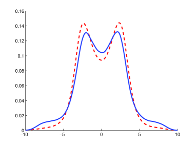
Figure 1: Approximate density of $\nu_{0}^{H}$ (continuous line) compared with that of $\nu^{\frac{1}{2}}_{0}$ (dotted line)

Finally, in order to have a rough idea of the rate of convergence, we depict in Figure 2 the approximate densities for different values of $n$ keeping the other parameters unchanged.

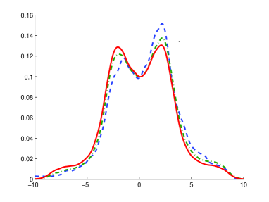
Figure 2: Approximate density of $\nu_{0}^{H}$ for $n=10^{5}$ (dotted line), $n=10^{6}$ (dash-dotted line), $n=10^{7}$ (continuous line)

REMARK 7.

As mentioned before, this section is only an illustration. In fact, there are (many) numerical open questions. For the estimation of the error, it would be necessary for a function $f$ to get some rate of convergence results for ${\cal P}^{(n,\gamma)}_{0}(f)-\nu_{H}(f)$ (long-time error) and for $\nu^{H,\gamma}_{0}(f)-\nu_{0}^{H}(f)$ (discretization error) where $\nu^{H,\gamma}_{0}$ denotes the initial distribution of the stationary Euler scheme with step $\gamma$. Note that in the diffusion case, it can be shown (under some appropriate assumptions that the long time error is about $(\gamma n)^{-\frac{1}{2}}$ (see [3] for the corresponding result in the continuous case) whereas the discretization error is $O(\gamma)$ (see [31], Theorem 3.3 for a similar result with the Milstein scheme). Finally, even if the Wood and Chan simulation method is fast and exact, it requires a lot of memory because of the Fast Fourier Transform. On Matlab, for instance, this implies that we can not take $n$ greater than $2.10^{7}$. Thus, it could be interesting to study some discretization schemes based on some approximations of the fBm-increments simulated, which consumes less memory.

7 Appendix

Proof of Proposition 2 Let us show that $(\bar{X}_{\gamma k})$ is a skew-product in the sense of [16] as follows. For a fractional Brownian $B^{H}$ motion on $\mathbb{R}$, set for every $n\in\mathbb{Z}$ $\Delta_{n}^{\gamma}=B^{H}_{(n+1)\gamma}-B^{H}_{n\gamma}$. Setting ${\cal W}:=(\mathbb{R}^{d})^{\mathbb{Z}_{-}}$, we then introduce the regular conditional probability $\bar{\cal P}^{\gamma}:{\cal W}\rightarrow{\cal M}_{1}(\mathbb{R}^{d})$ defined by:

$$\bar{\cal P}^{\gamma}(\omega)={\cal L}(\Delta_{1}^{\gamma}|(\Delta_{k}^{\gamma})_{k\leq 0}=\omega)$$

and denote by ${\cal P}^{\gamma}$ the Feller transition on ${\cal W}$ defined for every measurable function $f:{\cal W}\rightarrow\mathbb{R}$ by ${\cal P}^{\gamma}f(\omega)=\int_{\mathbb{R}^{d}}f(\omega\sqcup\tilde{\omega})\bar{\cal P}^{\gamma}(\omega,d\tilde{\omega})$ where for $\omega\in(\mathbb{R}^{d})^{\mathbb{Z}_{-}}$ and $\tilde{\omega}\in\mathbb{R}^{d}$, $\omega\sqcup\tilde{\omega}=(\ldots,\omega_{{}_{2}},\omega_{{}_{1}},\omega_{0},\tilde{\omega})$. Setting ${\Phi}^{\gamma}(x,\tilde{\omega})=x+\gamma b(x)+\sigma(x)\tilde{\omega}$ and $\mathbb{P}_{H}^{\gamma}:={\cal L}((\Delta_{n})_{n\leq 0})$, we have defined a skew-product $({\cal W},\mathbb{P}_{H}^{\gamma},{\cal P}^{\gamma},\mathbb{R}^{d},{\Phi}^{\gamma})$ with the transition operator ${\cal Q}^{\gamma}$ on $\mathbb{R}^{d}\times{\cal W}$ defined by

$${\cal Q}^{\gamma}f(x,\omega)=\int f(\Phi^{\gamma}(x,\omega^{\prime})){\cal P}^{\gamma}(\omega,d{\omega}^{\prime}),$$

which describes the dynamics of the Euler scheme.
Then, thanks to Theorem 1.4.17 of [16], uniqueness of the adapted and stationary discrete Euler scheme $(\bar{X}_{\gamma k})$ (in distribution) holds, if the skew-product $({\cal W},\mathbb{P}_{H}^{\gamma},{\cal P}^{\gamma},\mathbb{R}^{d},{\Phi}^{\gamma})$ is strong Feller and topologically irreducible (in the sense of Definition 1.4.6 and 1.4.7 of [16]).
First, write $\tilde{\omega}=(\tilde{\omega}^{1},\ldots,\tilde{\omega}^{q})$ and $\Phi^{\gamma}=(\Phi^{\gamma}_{1},\ldots,\Phi^{\gamma}_{d})$. Denote by $M^{\Phi}(x,\tilde{\omega})$ the (discrete) Malliavin covariance matrix of $\Phi$ defined by

$$\forall(x,\tilde{\omega})\in\mathbb{R}^{d}\times\mathbb{R}^{d}\quad\textnormal{and}(i,j)\in\{1,\ldots,d\}^{2},\quad M^{\Phi}_{i,j}(x,\tilde{\omega}):=\sum_{k=1}^{d}\partial_{\tilde{\omega}^{k}}\Phi^{\gamma}_{i}(x,\tilde{\omega})\partial_{\tilde{\omega}^{k}}\Phi^{\gamma}_{j}(x,\tilde{\omega}).$$

Thus, $M^{\Phi}(x,\tilde{\omega})=(\sigma\sigma^{*})(x)$ and since $\sigma^{-1}$ is bounded (and continuous), it follows that $x\rightarrow({\rm det}(M^{\Phi})^{-1}(x,\omega)$ is bounded continuous. Second, the functions $D_{\omega}\Phi$, $D_{\omega}D_{x}\Phi$ and $D^{2}_{\omega}\Phi$ are clearly bounded continuous. Finally, the sequence $((\Delta_{n}^{\gamma})^{1})$ has a spectral density $f$ that satisfies $\int_{-\pi}^{\pi}(f(x))^{-1}dx<+\infty$ (see $e.g.$ [2] for an explicit expression of $f$). Thus, it follows from Theorem 1.5.9 of [16] that the skew-product is strong Feller.
For the topological irreducibility, it is enough to show that for every $(x,\omega)\in\mathbb{R}^{d}\times{\cal W}$, for every $(y,\varepsilon)\in\mathbb{R}^{d}\times\mathbb{R}_{+}^{*}$, ${\cal Q}(x,\omega,B(y,\varepsilon)\times{\cal W})>0$ . Since $\sigma$ is invertible, the map $\Phi$ is controllable in the following sense: $\Phi(x,\tilde{\omega}_{x})=y$ has a (unique) solution $\tilde{\omega}\in\mathbb{R}^{q}$, for every $x,y\in\mathbb{R}^{d}$. Furthermore, $b$ and $\sigma$ being continuous, for every $\varepsilon>0$, there exists $r_{\varepsilon}$ such that for every $\tilde{\omega}\in B(\tilde{\omega}_{x},r_{\varepsilon})$, $\Phi(x,{\tilde{\omega}})\in B(y,\varepsilon)$. Thus

$${\cal Q}(x,\omega,B(y,\varepsilon)\times{\cal W})\geq\bar{\cal P}(\omega,B(\tilde{\omega}_{x},r_{\varepsilon}))>0,$$

since $\bar{\cal P}(\omega,.)$ is Gaussian with positive variance. This concludes the proof.

Acknowledgment

We would like to thank the anonymous referee for his/her careful reading and his/her suggestions that helped us to improve the first version of this article.

References

• [1] Ludwig Arnold. Random dynamical systems. Springer Monographs in Mathematics. Springer-Verlag, Berlin, 1998.
• [2] Jan Beran. Statistics for long-memory processes, volume 61 of Monographs on Statistics and Applied Probability. Chapman and Hall, New York, 1994.
• [3] R. N. Bhattacharya. On the functional central limit theorem and the law of the iterated logarithm for Markov processes. Z. Wahrsch. Verw. Gebiete, 60(2):185–201, 1982.
• [4] Patrick Cheridito, Hideyuki Kawaguchi, and Makoto Maejima. Fractional Ornstein-Uhlenbeck processes. Electron. J. Probab., 8:no. 3, 14 pp. (electronic), 2003.
• [5] Serge Cohen and Fabien Panloup. Approximation of stationary solutions of Gaussian driven stochastic differential equations. Stochastic Process. Appl., 121(12):2776–2801, 2011.
• [6] Laure Coutin. Rough paths via sewing lemma. ESAIM PS, 16:479–526, 2012.
• [7] Hans Crauel. Non-Markovian invariant measures are hyperbolic. Stochastic Process. Appl., 45(1):13–28, 1993.
• [8] A. M. Davie. Differential equations driven by rough paths: an approach via discrete approximation. Appl. Math. Res. Express. AMRX, (2):Art. ID abm009, 40, 2007.
• [9] A. Deya, A. Neuenkirch, and S. Tindel. A Milstein-type scheme without Lévy area terms for SDEs driven by fractional Brownian motion. Ann. Inst. Henri Poincaré Probab. Stat., 48(2):518–550, 2012.
• [10] Marie Duflo. Random iterative models, volume 34 of Applications of Mathematics (New York). Springer-Verlag, Berlin, 1997. Translated from the 1990 French original by Stephen S. Wilson and revised by the author.
• [11] Denis Feyel and Arnaud de La Pradelle. Curvilinear integrals along enriched paths. Electron. J. Probab., 11:no. 34, 860–892 (electronic), 2006.
• [12] Peter K. Friz and Nicolas B. Victoir. Multidimensional stochastic processes as rough paths, volume 120 of Cambridge Studies in Advanced Mathematics. Cambridge University Press, Cambridge, 2010. Theory and applications.
• [13] María J. Garrido-Atienza, Peter E. Kloeden, and Andreas Neuenkirch. Discretization of stationary solutions of stochastic systems driven by fractional Brownian motion. Appl. Math. Optim., 60(2):151–172, 2009.
• [14] Paolo Guasoni. No arbitrage under transaction costs, with fractional Brownian motion and beyond. Math. Finance, 16(3):569–582, 2006.
• [15] Martin Hairer. Ergodicity of stochastic differential equations driven by fractional Brownian motion. Ann. Probab., 33(2):703–758, 2005.
• [16] Martin Hairer. Ergodic properties of a class of non-Markovian processes. In Trends in stochastic analysis, volume 353 of London Math. Soc. Lecture Note Ser., pages 65–98. Cambridge Univ. Press, Cambridge, 2009.
• [17] Martin Hairer and Alberto Ohashi. Ergodic theory for SDEs with extrinsic memory. Ann. Probab., 35(5):1950–1977, 2007.
• [18] Jae-Hyung Jeon, Vincent Tejedor, Stas Burov, Eli Barkai, Christine Selhuber-Unkel, Kirstine Berg-Sørensen, Lene Oddershede, and Ralf Metzler. In Vivo anomalous diffusion and weak ergodicity breaking of lipid granules. Phys. Rev. Lett., 106:048103, Jan 2011.
• [19] S. C. Kou. Stochastic modeling in nanoscale biophysics: subdiffusion within proteins. Ann. Appl. Stat., 2(2):501–535, 2008.
• [20] Damien Lamberton and Gilles Pagès. Recursive computation of the invariant distribution of a diffusion. Bernoulli, 8(3):367–405, 2002.
• [21] Damien Lamberton and Gilles Pagès. Recursive computation of the invariant distribution of a diffusion: the case of a weakly mean reverting drift. Stoch. Dyn., 3(4):435–451, 2003.
• [22] Vincent Lemaire. An adaptive scheme for the approximation of dissipative systems. Stochastic Process. Appl., 117(10):1491–1518, 2007.
• [23] Terry Lyons. Differential equations driven by rough signals. I. An extension of an inequality of L. C. Young. Math. Res. Lett., 1(4):451–464, 1994.
• [24] Benoit B. Mandelbrot and John W. Van Ness. Fractional Brownian motions, fractional noises and applications. SIAM Rev., 10:422–437, 1968.
• [25] Gisirō Maruyama. The harmonic analysis of stationary stochastic processes. Mem. Fac. Sci. Kyūsyū Univ. A., 4:45–106, 1949.
• [26] David Nualart and Aurel Răşcanu. Differential equations driven by fractional Brownian motion. Collect. Math., 53(1):55–81, 2002.
• [27] David J. Odde, Elly M. Tanaka, Stacy S. Hawkins, and Helen M. Buettner. Stochastic dynamics of the nerve growth cone and its microtubules during neurite outgrowth. Biotechnology and Bioengineering, 50(4):452–461, 1996.
• [28] Gilles Pagès and Fabien Panloup. Approximation of the distribution of a stationary Markov process with application to option pricing. Bernoulli, 15(1):146–177, 2009.
• [29] Fabien Panloup. Recursive computation of the invariant measure of a stochastic differential equation driven by a Lévy process. Ann. Appl. Probab., 18(2):379–426, 2008.
• [30] Alfredas Račkauskas and Charles Suquet. Central limit theorem in Hölder spaces. Probab. Math. Statist., 19(1, Acta Univ. Wratislav. No. 2138):133–152, 1999.
• [31] Denis Talay. Second order discretization schemes of stochastic differential systems for the computation of the invariant law. Stoch. Stoch. Rep., 29(1):13–35, 1990.
• [32] Michel Weber. Sur un théorème de Maruyama. In Seminar on Probability, XIV (Paris, 1978/1979) (French), volume 784 of Lecture Notes in Math., pages 475–488. Springer, Berlin, 1980.
• [33] Andrew T. A. Wood and Grace Chan. Simulation of stationary Gaussian processes in $[0,1]^{d}$. J. Comput. Graph. Statist., 3(4):409–432, 1994.
• [34] L. C. Young. An inequality of the Hölder type, connected with Stieltjes integration. Acta Math., 67(1):251–282, 1936.