Active plasma resonance spectroscopy:
A functional analytic description

Abstract

The term “Active Plasma Resonance Spectroscopy” denotes a class of diagnostic methods which employ the ability of plasmas to resonate on or near the plasma frequency. The basic idea dates back to the early days of discharge physics: A signal in the GHz range is coupled to the plasma via an electrical probe; the spectral response is recorded, and then evaluated with a mathematical model to obtain information on the electron density and other plasma parameters. In recent years, the concept has found renewed interest as a basis of industry compatible plasma diagnostics. This paper analyzes the diagnostics technique in terms of a general description based on functional analytic (or Hilbert Space) methods which hold for arbitrary probe geometries. It is shown that the response function of the plasma-probe system can be expressed as a matrix element of the resolvent of an appropriately defined dynamical operator. A specialization of the formalism to a symmetric probe design is given, as well as an interpretation in terms of a lumped circuit model consisting of series resonance circuits. We present ideas for an optimized probe design based on geometric and electrical symmetry.

I Introduction

Of the many diagnostic techniques available or proposed for low temperature plasmas, only a few are compatible with industrial requirements. A diagnostic tool which is useful for supervision and/or control of technological plasma processes must be i) robust and stable, ii) insensitive against perturbation by the process, iii) itself not perturbing to the process, iv) clearly and easily interpretable without the need of calibration, v) compliant with the requirements of process integration, and, last not least, vi) economical in terms of investment, footprint, and maintenance.

In this paper we focus on a very promising approach to industry compatible plasma diagnostics, the so-called plasma resonance spectroscopy. This approach attempts to exploit the natural ability of plasmas to resonate on or near the electron plasma frequency $\omega_{\rm pe}=\sqrt{e^{2}n_{\rm e}/\epsilon_{0}m_{\rm e}}$ for diagnostics purposes. The idea to use these resonances to determine plasma parameters dates back to the early days of discharge physics tonks1929 and has found many different realizations since then takayama1960 ; stenzel1960 ; cohen71 ; klick1996 ; sugai1999 ; nakamura2003 ; kim2003 ; piejak2004 ; franz2005 ; booth2005 ; scharwitz2008 ; scharwitz2009 ; li2010 ; wang2011 . We follow the classification of lapke11 : Active plasma resonance spectroscopy couples a suitable RF signal into the plasma and records the response takayama1960 ; stenzel1960 ; cohen71 ; sugai1999 ; nakamura2003 ; kim2003 ; piejak2004 ; booth2005 ; scharwitz2008 ; scharwitz2009 ; li2010 ; wang2011 . Passive plasma resonance spectroscopy merely observes the pre-existing excitation of the plasma by other sources (typically, the RF power input) klick1996 ; franz2005 . Electromagnetic concepts are based on the interaction of the plasma with the full electromagnetic field, they operate above the plasma frequency and observe the plasma-induced shift of transmission line or cavity resonances which are already present in vacuum stenzel1960 ; kim2003 ; piejak2004 ; wang2011 . Electrostatic concepts, on the other hand, result from the interaction of the plasma with the electric field alone; they utilize resonances below $\omega_{\rm pe}$ which are not present in vacuum (standing surfaces waves) and deduce the plasma parameters from the absolute value of the frequency takayama1960 ; cohen71 ; sugai1999 ; nakamura2003 ; booth2005 ; scharwitz2008 ; scharwitz2009 ; li2010 . Finally, one-port concepts utilize probes with only one electrical input/output port takayama1960 ; cohen71 ; klick1996 ; sugai1999 ; nakamura2003 ; piejak2004 ; franz2005 ; scharwitz2008 ; scharwitz2009 ; li2010 ; wang2011 , while two-port concepts use a probe configuration with two ports or even two separate probes stenzel1960 ; kim2003 ; piejak2004 ; booth2005 . (Multi-port concepts would also be conceivable.)

Many groups have dealt with simulation and modeling of specialized aspects of such diagnostic devices to achieve a better understanding of the resonance behavior booth2005 ; scharwitz2008 ; xu2009 ; xu2010 ; bin2010 ; liang2011 . In contrast, the purpose of this manuscript is to study the whole class of active, electrostatic methods in order to gain a deeper physical understanding of the resonance behavior. Therefore, we use a general description based on functional analytic methods which allows for an analysis without particular assumptions on the probe geometries or the homogeneity of the plasma.

II A model of an electrostatic probe in arbitrary geometry

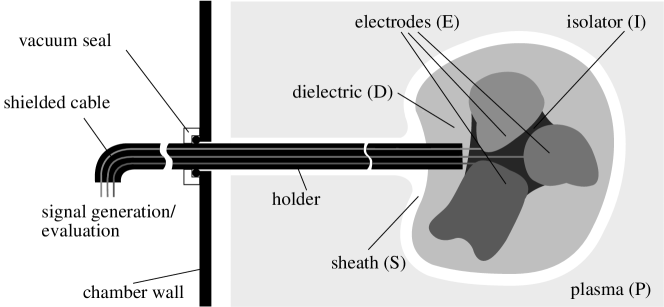
Figure 1: Illustration of the abstract model for a N-electrode system. The electrodes are shielded to each other and the plasma by some dielectric medium. The whole probe, surrounded by a plasma sheath is immersed in a plasma volume.

We represent the plasma chamber (see figure 1) as a simply connected, spatially bounded domain $V$, most of which is plasma (a simply connected subdomain $P$). Other subdomains of $V$ are the plasma boundary sheath $S$, which shields the plasma from all material objects, and possibly dielectric domains $D$. The boundary $\partial V$ of the domain $V$ is either grounded ($G$) or ideally insulating ($I$) with vanishing conductivity and permittivity.

Into this idealized plasma chamber, a diagnostic device is immersed. To render our considerations general, we assume that it is a probe of arbitrary shape, containing an arbitrary number of powered electrodes. The electrodes surfaces $E_{k}$, $k=1\dots N$ are also seen as part of the domain boundary $\partial V$, of course they are insulated from each other and from ground. A possible dielectric shielding of the probe is represented as a part of the subdomain $D$ within the plasma chamber $V$. Fig. 1 illustrates the assumed geometry.

Within the subdomain $P$, the plasma is described by the cold plasma model, a set of two coupled linear equations for the RF charge density $\rho$ and the RF current density $\vec{j}$. The first expresses the conservation of charge, the second describes the acceleration of the electron fluid by the RF electric field $\vec{E}=-\nabla\Phi$ and the momentum loss due to electron-neutral collisions (measured by its rate $\nu$),

$$\frac{\partial\rho}{\partial t}+\nabla\!\cdot\!\vec{j}=0,$$ (1)

$$\frac{\partial\vec{j}}{\partial t}=-\epsilon_{0}\omega_{\rm pe}^{2}\nabla\Phi-\nu{\vec{j}}.$$ (2)

The electric potential $\Phi$ is not only defined in the plasma domain $P$, but also in the sheath $S$and in the dielectric $D$. RF charges are present in the plasma $P$ and – as surface charges – on the plasma boundary $\partial P$. The sheath, however, is electron-free and hence RF charge free. Consequently, Poisson’s equation gives the RF potential as

$$-\nabla\!\cdot\!\left(\epsilon_{0}\epsilon\nabla\Phi\right)=\left\{\begin{array}[]{ll}\rho&\hbox{in the plasma $P$ and on $\partial P$, }\\[2.15277pt] 0&\hbox{in dielectric domains $D$ and the sheath $S$.}\\ \end{array}\right.$$ (3)

The permittivity is given by

$$\epsilon=\epsilon{(\vec{r})}=\left\{\begin{array}[]{ll}1&\hbox{in the plasma $P$ and the sheath $S$, }\\ \epsilon_{r}(\vec{r})&\hbox{in dielectric domains $D$.}\end{array}\right.$$ (4)

The electrodes $E_{k}$ are driven by RF voltages $V_{k}$, with $k=1\dots N$. On the grounded parts of the wall or the probes the potential vanishes. It is convenient to treat these sections as a further electrode $E_{0}$ with an applied voltage $V_{0}=0$. Taking also into account the insulating surfaces $I$, the boundary conditions for the potential are of mixed type:

$$\begin{array}[]{l@{\;\;\;\;\;}l}\text{Electrodes $E_{k}$:}&\Phi|_{E_{k}}=V_{k},\;\;\;\;\;k=0\ldots N\\ \text{Insulators $I$:}&\vec{n}\!\cdot\!\nabla\Phi|_{I}=0.\end{array}$$ (5)

The currents $I_{k}$ carried by the electrodes are the measured signals of the diagnostic. As the electrodes are shielded from the plasma, at least by the sheath, the currents are carried by displacement alone. Counting them positive when they flow from the electrode to the plasma (in the direction of the negative surface normal), one obtains

$$I_{k}=\int_{E_{k}}\epsilon_{0}\epsilon_{r}\frac{\partial\nabla\!\Phi}{\partial t}\,\!\cdot\!\,d^{2}\vec{r}.$$ (6)

Of course, there is a standard approach to solve these equations: Applying the Fourier transform to the equation of motion leads to the RF version of Ohms law, an expression of the total current in terms of the field. The model reduces to an elliptic equation in the domain $V$,

$$\nabla\!\cdot\!\left(\epsilon_{0}\epsilon^{\rm(eff)}\nabla\Phi\right)=0,$$ (7)

with the effective permittivity $\epsilon^{\rm(eff)}$ given by

$$\epsilon^{\rm(eff)}=\left\{\begin{array}[]{ll}1-\frac{\displaystyle\omega_{\rm pe}^{2}}{\displaystyle\omega(\omega-i\nu)}&\hbox{in the plasma $P$, }\\[2.15277pt] 1&\hbox{in the sheath $S$,}\\[2.15277pt] \epsilon_{r}(\vec{r})&\hbox{in dielectric domains $D$.}\end{array}\right.$$ (8)

Together with the Fourier transformed boundary conditions (5), the elliptic equation can easily be solved numerically. Its linearity allows to write the solution $\Phi(\vec{r})$ as a superposition of $N$ fundamental solutions,

$$\Phi(\vec{r})=\sum_{l=1}^{N}V_{l}\Phi_{l}(\vec{r}).$$ (9)

each of which obeys equation (7) and the boundary conditions ($\delta_{kl}$ is Kronecker’s delta)

$$\begin{array}[]{l@{\;\;\;\;\;}l}\text{Electrode $E_{k}$:}&\Phi_{l}|_{E_{k}}=\delta_{kl},\;\;\;\;\;l=0\ldots N,\\ \text{Insulators:}&\vec{n}\!\cdot\!\nabla\Phi_{l}|_{\partial I}=0.\end{array}$$ (12)

With the help of the fundamental solutions $\Phi_{l}$, a response matrix $Y_{kl}$ can be defined as the flux of the Fourier transformed displacement current through electrode $E_{k}$,

$$Y_{kl}=\int_{E_{k}}i\omega\epsilon_{0}\epsilon^{\rm(eff)}\nabla\Phi_{l}\,\!\cdot\!d^{2}\vec{r}\,.$$ (13)

The Fourier transformed RF current $I_{k}$ as the probe signal can then be calculated as

$$I_{k}=\sum_{l=1}^{N}Y_{kl}V_{l},.$$ (14)

This approach has been successfully employed for numerical investigations of the plasma absorption probe and the multipole resonance probe in lapke08 and lapke07 . It relies, however, on numerical calculations and gives only a limited insight into physics of the probe response: Although the mathematical structure of (7) to (14) is quite transparent, it is not possible to separate the plasma contributions from the influences of the geometry from the numerical solution.

III Current and energy balance equations

In order to obtain a deeper understanding of the probe model behavior, we focus on the balance equations of current and energy and continue with a general formalism. To make this section more readable some derivations are shifted to the appendix. We split the electric potential into two parts, one of which is the vacuum potential which can be written as a linear superposition of characteristic functions,

$$\Phi(\vec{r})=\phi(\vec{r})+\Phi^{\rm(vac)}(\vec{r})=\phi(\vec{r})+\sum_{l=0}^{N}V_{l}\Psi_{l}(\vec{r})\,.$$ (15)

The characteristic functions $\Psi_{l}$, with $l=0\dots N$, depend only on the geometry of the chamber and the geometry of the probe. They are independent of the plasma and its spatial distribution. To calculate the $\Psi_{l}$, the related Laplace equation has to be solved, i.e.

$$\nabla\!\cdot\!\left(\epsilon_{0}\epsilon_{r}\nabla\Psi_{l}\right)=0\ .$$ (16)

The boundary conditions are given by

$$\begin{array}[]{l@{\;\;\;\;\;}l}\text{Electrode $E_{k}$:}&\Psi_{l}|_{E_{k}}=\delta_{kl},\;\;\;\;\;l=0\ldots N,\\ \text{Insulators:}&\vec{n}\!\cdot\!\nabla\Psi_{l}|_{\partial I}=0.\end{array}$$ (19)

The first part of the electric potential defined in (15), referred as the inner potential $\phi$, is given by Poisson’s equation in the plasma and the sheath, or dielectric zones, and satisfies homogeneous boundary conditions. One obtains the boundary value problem

$$-\nabla\!\cdot\!\left(\epsilon_{0}\epsilon_{r}\nabla\phi\right)=\left\{\begin{array}[]{ll}\rho&\hbox{in the plasma $P$ and on $\partial P$, }\\[2.15277pt] 0&\hbox{in dielectric domains $D$ and the sheath $S$,}\\[2.15277pt] \end{array}\right.$$ (22)

$$\begin{array}[]{l@{\;\;\;\;\;}l}\text{Electrode $E_{k}$:}&\phi|_{E_{k}}=0,\;\;\;\;\;k=0\ldots N,\\ \text{Insulator:}&\vec{n}\!\cdot\!\nabla\phi|_{\partial I}=0.\end{array}$$ (25)

With the knowledge of the two distinct parts of the potential, we are able to reformulate dynamical equations for the charge density and the current density. From (1) and (2) we ultimately arrive at

$$\frac{\partial\rho}{\partial t}=-\nabla\!\cdot\!\vec{j},$$ (26)

$$\frac{\partial\vec{j}}{\partial t}=-\epsilon_{0}\omega_{\rm pe}^{2}\nabla\phi-\nu{\vec{j}}-\epsilon_{0}\omega_{\rm pe}^{2}\sum_{l=0}^{N}V_{l}\nabla\Psi_{l}.$$ (27)

Similarly to the potential, the current $I_{k}$ carried by the electrode $E_{k}$ can also be split into two parts, $I_{k}(t)=i_{k}(t)+I_{k}^{\rm(vac)}(t)$. The first term is referred to as the inner current, the second is the vacuum part. The vacuum part is nothing but the displacement current related to the vacuum field $\Phi^{\rm(vac)}$. It is shown in the appendix that it has a purely capacitive character. One obtains

$$I_{k}^{\rm(vac)}=-\sum_{l=0}^{N}C_{kl}\frac{\partial V_{l}}{\partial t}.$$ (28)

The coefficients $C_{kl}$ are the capacitance coefficients defined by

$$C_{kl}=\int_{\partial V}\Psi_{k}\epsilon_{0}\epsilon_{r}\nabla\Psi_{l}\!\cdot\!d^{2}\vec{r}.$$ (29)

It is also shown in the appendix that the vacuum current satisfies Kirchhoff’s law of current conservation, i.e., the sum of the currents over all electrodes (including grounded electrodes) is equal to zero,

$$\sum_{k=0}^{N}I_{k}^{\rm(vac)}=\sum_{k=0}^{N}\sum_{l=0}^{N}C_{kl}\frac{\partial V_{l}}{\partial t}=0.$$ (30)

With the help of the characteristic functions introduced in the previous section, the inner part of the current $i_{k}$ can be written as a flux integral over the electrode $E_{k}$

$$i_{k}=-\int_{V}\nabla\Psi_{k}\!\cdot\!\vec{j}\,d^{3}r.$$ (31)

(Again the explicit derivation can be found in the appendix.) The inner part of the current obeys Kirchhoff’s law of current conservation, i.e., their sum over all electrodes (including ground electrodes) is equal to zero (see also appendix).

We now establish energy balance equations for the system. Owing to the fact that the coupling of the vacuum field and the inner potential vanishes (see appendix), we can split the electrical energy of the system into a vacuum part $E^{\rm(vac)}$ and an inner part $\varepsilon^{\rm(el)}$ given by

$$\varepsilon^{\rm(el)} = \int_{V}\frac{1}{2}\epsilon_{0}\epsilon_{r}\nabla\phi\!\cdot\!\nabla\phi\,d^{3}r$$ (32)

and

$$E^{\rm(\rm vac)}=\frac{1}{2}\sum_{k=0}^{N}\sum_{l=0}^{N}C_{kl}V_{k}V_{l}\,.$$ (33)

The vacuum part can be expressed in terms of the previously defined capacitance coefficients (29). Its derivative with respect to time simply describes the charging and decharging of the linear multiport capacitor $C_{kl}$,

$$\frac{dE^{\rm(vac)}}{dt}=\sum_{k=0}^{N}\sum_{l=0}^{N}C_{kl}V_{k}\frac{\partial V_{l}}{\partial t}=\sum_{l=0}^{N}V_{l}I^{\rm(vac)}.$$ (34)

The inner energy $\varepsilon$ is the sum of the inner electrical energy $\epsilon^{\rm(el)}$ and the kinetic energy due to the motion of electrons

$$\varepsilon=\varepsilon^{\rm(el)}+\varepsilon^{\rm(kin)}=\int_{V}\frac{1}{2}\epsilon_{0}\epsilon_{r}\nabla\phi\!\cdot\!\nabla\phi\,d^{3}r+\int_{P}\frac{1}{2\epsilon_{0}\omega_{\rm pe}^{2}}\vec{j}^{\,2}\,d^{3}r.$$ (35)

The temporal change in the inner energy is governed by the balance of the power input and the Ohmic dissipation due to collisions

$$\frac{d\varepsilon}{dt}=\sum_{l=0}^{N}V_{l}i_{l}-\int_{P}\frac{\nu}{\epsilon_{0}\omega_{\rm pe}^{2}}\vec{j}^{2}\,d^{3}r.$$ (36)

IV A lumped element analogy

As a simple problem and to introduce an abstract mathematical formulation, we consider the response of a lumped series resonance circuit driven by a voltage $V(t)$ as shown in figure 2. One can interpret this scenario as a one-port concept which does not couple to the outer ground. We assume the values of the lumped circuit elements as given. (To evaluate real plasma diagnostic concepts the values have of course to be determined by means of a mathematical model.)

The exemplary model can be cast as a system of two coupled ordinary differential equations of first order for the capacitor voltage $U$ and the current $I$,

$$\frac{dU}{dt} = \frac{I}{C},$$ (37)

$$\frac{dI}{dt} = -\frac{U}{L}-\frac{RI}{L}+\frac{1}{L}V(t).$$ (38)

To solve the system the Fourier transform can be used and one obtains its admittance that is interpretable as the system response of the one-port probe

$$Y(\omega)=\frac{I}{V}=\displaystyle\frac{\displaystyle 1}{\displaystyle R+i\omega L+\frac{\displaystyle 1}{\displaystyle i\omega C}}.$$ (39)

The same result can be derived by an abstract mathematical formulation of the system. To introduce this formulation we refer to the ordered pair of $U$ and $I$ as the state of the system, denoted by the state vector

$$|z\rangle\equiv|U,I\rangle=\left(\!\begin{array}[]{c}U\\ I\end{array}\!\right).$$ (40)

Similarly, we introduce the vector of the excitation of the system

$$|e\rangle=\left(\!\begin{array}[]{c}0\\ \displaystyle\frac{1}{L}\end{array}\!\right).$$ (41)

The operators of the non-dissipative and the dissipative dynamics are given by

$$T_{C}=\left(\begin{array}[]{cc}0&\displaystyle\frac{1}{C}\\ -\displaystyle\frac{1}{L}&0\end{array}\right),\qquad T_{D}=\left(\begin{array}[]{cc}0&0\\ 0&-\displaystyle\frac{R}{L}\end{array}\right).$$ (42)

With the help of these definitions, the behavior of the lumped element circuit can be expressed in terms of a compact dynamic equation,

$$\frac{d|z\rangle}{dt}=T_{\rm C}|z\rangle+T_{\rm D}|z\rangle+V(t)|e\rangle.$$ (43)

Since the set of all states $|z\rangle$ forms a vector space $Z$ it is advantageous to employ as the underlying scalar field the set of complex numbers $\mathbb{C}$. To turn $Z$ into a Hilbert space, the appropriate scalar product has to be defined. Due to the fact that the dimension of the vectors $|z\rangle$ is inhomogeneous, the Euclidian product is not available. However, a physically reasonable quadratic form exists, i.e., the energy $\varepsilon=\left(CU^{2}+LI^{2}\right)/2$, which is stored in the capacitance and the inductance of the resonant circuit. This motivates the definition of a scalar product of two state vectors $|\tilde{z}\rangle$ and $|z\rangle$ as

$$\langle\tilde{z}|z\rangle\equiv\langle\tilde{U},\tilde{I}|U,I\rangle:=C{\tilde{U}}^{*}U+L{\tilde{I}}^{*}I.$$ (44)

The energy is a non-negative real quantity even for complex states,

$$\varepsilon=\frac{1}{2}\left\|z\right\|^{2}=\frac{1}{2}\langle z|z\rangle.$$ (45)

The defined scalar product is compatible with the dynamical equations. It can be shown that the operator $T_{C}$ is anti-Hermitian with respect to the scalar product,

$$\langle T_{C}\tilde{z}|z\rangle=-\langle\tilde{z}|T_{C}z\rangle,$$ (46)

while the dissipative operator $T_{D}$ is Hermitian and negative definite,

$$\langle T_{D}\tilde{z}|z\rangle = \langle\tilde{z}|T_{D}|z\rangle,$$ (47)

$$\langle\tilde{z}|T_{C}|z\rangle \leq 0.$$ (48)

Furthermore, it can be shown that the observable response of the system, i.e., the current $I$, is the scalar product of the excitation vector and the state vector $|z\rangle$. Thus, the observation vector is equal to the excitation vector,

$$I=\langle 0,{\frac{\displaystyle 1}{\displaystyle L}}|U,I\rangle=\langle e|z\rangle.$$ (49)

The energy balance equation (45) can be transformed to the energy balance equation of a series resonance circuit

$$\frac{d}{dt}\left(\frac{1}{2}CU^{2}+\frac{1}{2}LI^{2}\right)=-RI^{2}+I\,V(t).$$ (50)

To analyze the response of the system we apply the Fourier transform to (43). The current is then given by

$$I=\langle e|z\rangle=\langle e|\frac{1}{\displaystyle i\omega-T_{\rm C}-T_{\rm D}}|e\rangle V(\omega)=Y(\omega)V.$$ (51)

The response function $Y(\omega)$ of the system can be directly specified by evaluating the matrix products. It should be noted, that two extra matrices from the scalar product (44) appear in the calculation. However, the response function can also be calculated by expanding the state vectors into the eigenfunctions of the operator. One ultimately obtains exactly the same expresion than in (39). This result of the simple RCL-series circuit allows the physical interpretation of the abstract solution that is derived in a section further down.

V Functional analytic formulation of the probe response

We are now equipped with all the material necessary for a functional analytic formulation of the system of dynamical equations (26) and (27). We interpret the charge density $\rho(\vec{r})$ and the current density $\vec{j}(\vec{r})$ defined on the plasma domain $P$ as the variables of the system state $|z\rangle$. (It is advantageous to allow for complex states.) In Dirac’s bra-ket notation we define an appropriate function space as

$${\mathcal{H}}=\left\{|z\rangle\equiv|\rho,\vec{j}\rangle\equiv(\rho,\vec{j})^{\rm T}\right\}.$$ (52)

For two system states $|z\rangle\equiv|\rho,\vec{j}\rangle$ and $|z^{\prime}\rangle\equiv|\rho^{\prime},\vec{j}^{\prime}\rangle$ we define a scalar product $\left\langle z|z^{\prime}\right\rangle$ which is motivated by the inner energy functional (35). The following Hermitian form is compatible with the dynamical equations and satisfies all requirements of an inner product, namely i) conjugate symmetry, ii) sesquilinearity, and iii) positive definiteness.

$$\left\langle z|z^{\prime}\right\rangle=\int_{V}\epsilon_{0}\,\epsilon_{r}\nabla\phi\{\rho\}^{*}\!\cdot\!\nabla\phi\{\rho^{\prime}\}\,d^{3}r+\int_{P}\frac{1}{\epsilon_{0}\omega_{\rm pe}^{2}}\vec{j}^{*}\!\cdot\!\vec{j}^{\prime}\,d^{3}r\,.$$ (53)

The scalar product defines a corresponding norm $\left\|z\right\|$. The norm-square of a state is equal to its inner energy, up to a factor of two

$$\left\|z\right\|^{2}=\left\langle z|z\right\rangle=\int_{V}\epsilon_{0}\,\epsilon_{r}\nabla\phi\{\rho\}^{*}\!\cdot\!\nabla\phi\{\rho\}\,d^{3}r+\int_{P}\frac{1}{\epsilon_{0}\omega_{\rm pe}^{2}}\vec{j}^{*}\!\cdot\!\vec{j}\,d^{3}r=2\varepsilon\,.$$ (54)

Equipped with this scalar product, and suitably completed, the defined function space of all possible states forms a Hilbert space $\mathcal{H}$. It should be noted that the elements of $\mathcal{H}$ are not all regular functions. The charge part may contain also singular functions like surface charges. However, this is acceptable as long as the norm $\left\|z\right\|$ is finite.

One important family of states $|e_{k}\rangle$ can be obtained from the characteristic vacuum functions $\Psi_{k}$ which have only a current part, their charge part and also the corresponding potential are equal to zero,

$$|e_{k}\rangle=|0,-\epsilon_{0}\omega_{\rm pe}^{2}\nabla\Psi_{k}\rangle.$$ (55)

The scalar product of $|e_{k}\rangle$ with a system state $|z\rangle$ is an expression for the inner current $i_{k}$ which is carried by the electrode $E_{k}$. Utilizing the definition of the scalar product (54) one obtains

$$\langle e_{k}|z\rangle=\int_{V}\nabla\Psi_{k}\!\cdot\!\vec{j}\,d^{3}r=i_{k}.$$ (56)

The dynamical equations (26) and (27) can be written in a compact form mussenbrock2007 . We define two dynamical operators $T_{C}$ and $T_{D}$ which act on the Hilbert space $\mathcal{H}$. The conservative operator $T_{C}$ contains the effects of the electron inertia and the electric field; it is defined by the action

$$T_{C}|\rho,\vec{j}\rangle=|-\nabla\!\cdot\!\vec{j},-\epsilon_{0}\omega_{\rm pe}^{2}\nabla\phi\{\rho\}\rangle.$$ (57)

$T_{C}$ can be shown to be anti-Hermitian, i.e., $T_{C}=-T_{C}^{\dagger}$ (see appendix). Thus the associated eigenvalues are purely imaginary and represent the frequency behavior. The dissipative operator $T_{D}$ contains the effects of the collisions

$$T_{D}|\rho,\vec{j}\rangle=|0,-\nu\vec{j}\rangle.$$ (58)

It can be shown that $T_{D}$ is Hermitian, i.e., $T_{D}=T_{D}^{\dagger}$ (see appendix). The eigenvalues are negative definite, $\left\langle z|T_{D}|z\right\rangle\leq 0$. Furthermore, they are real and contain information about damping of the system. With the help of these definitions, the dynamical equations (26) and (27) of the system can be written as

$$\frac{\partial|z\rangle}{\partial t}=T_{C}|z\rangle+T_{D}|z\rangle+\sum_{l=0}^{N}V_{l}|e_{l}\rangle.$$ (59)

Applying a Fourier transform to this abstract form and solving for $|z\rangle$, the measured current can be obtained

$$i_{k}=\langle e_{k}|z\rangle=\sum_{l=1}^{N}\langle e_{k}|\left(i\omega-T_{C}-T_{D}\right)^{-1}|e_{l}\rangle V_{l}=\sum_{l=1}^{N}y_{kl}V_{l}\ .$$ (60)

Thus, the response function, can be written as

$$y_{kl}(\omega)=\langle e_{k}|\left(i\omega-T_{C}-T_{D}\right)^{-1}|e_{l}\rangle.$$ (61)

The main result of this analysis is that the response function $y_{kl}(\omega)$ is given by the matrix elements of the resolvent of the dynamical operator equation evaluated for values on the imaginary axis. The result can be ultimately interpreted using equivalent lumped element circuits as described above.

VI Results for a one-port probe

With this result and the insights gained from the simple application of the formulated theory, we are able to discuss the result of the abstract model, given by equation (60) in terms of a lumped element circuit model. For a one-port probe (we account for two electrodes plus ground) the current to one of the two powered electrodes is given as

$$i_{k}=\langle e_{k}|z\rangle=\sum_{l=0}^{2}\langle e_{k}|\left(i\omega-T_{C}-T_{D}\right)^{-1}|e_{l}\rangle V_{l}=\sum_{l=0}^{2}y_{kl}V_{l}.$$ (62)

Comparing the response function $y_{kl}(\omega)$ (61) with the one in (51) reveals the same structure. It represents the coupling between the powered electrodes directly and the coupling from each electrode to ground. In this case, the dynamical operator $T=T_{C}+T_{D}$ is not a matrix as in the simple example, but a functional operator. The current is able to flow on infinite different paths through the plasma, each path can be expressed by a series resonance circuit. Therefore, the response function represents an infinite number of series resonance circuits connected in parallel.

In summary, the complete equivalent circuit consists of a branch which represents the direct coupling between the two powered electrodes. Two additional branches mimic the parasitic coupling of the electrodes to ground or “infinity”. Each branch itself is complex, and the relation between the plasma and probe parameters and the values of the circuit elements are generally very complicated. This case is depcited in figure 3. For realizations with more than one port the coupling gets even more complex.

Under strictly electrical and geometrical symmetry the situation for a one-port probe becomes simpler. It can be shown via a $\Delta$-Y transform (circuit theory) that the coupling to ground or “infinity” vanishes. As the field decays quickly with increasing distance from the probe, the measurements become actually local. The equivalent circuit becomes more simple: an infinite number of series resonance circuits, each of which representing a discrete resonance mode, are connected in parallel to a vacuum coupling.

The multipole resonance probe proposed by the authors lapke08 fulfills these requirements to a great extent – it consists of two separated hemispherical electrodes covered by a dielectric shielding. Thus its geometry is approximately symmetric (with respect to rotations around the center of the probe) and its electrical behavior is completely symmetric (with respect to the mapping $\omega t\rightarrow\omega t+\pi$ and $\Phi\rightarrow-\Phi$. Additionally, the spherical geometry allows for a compact mathematical description of the resonance behavior and simple algebraic expression for its resonance frequencies.

VII Summary / Conclusion / Outlook

We have formulated a model of electrostatic active resonance spectroscopic methods in terms of a functional analytic approach. The abstract character of these methods allow for a generalized model where the geometrical and electrical details of the probe realization do not enter explicitly in the equations. We presented a general analytic solution for the system state that gives physical insight in the resonance behavior. The scalar product between this state and the observation vector was shown to be the inner current at one electrode. Part of the current is the inner admittance that is determined as a matrix element by the resolvent and the observation vector. This result can be interpreted in terms of a lumped element equivalent circuit. To guide the physical interpretation of the functional analytic approach this method was explicitly used to obtain the systems response of a idealized situation, i.e., that the equivalent circuit is described by a simple RCL-series circuit.

As an example we presented the equivalent circuit of an one-port probe. An analysis of this circuit allows for an optimization of the probe geometry. Due to a symmetrical geometry and a symmetrical applied voltage it is possible to transform the circuit in an equivalent circuit of one branch between the two electrodes. This branch is given by an infinite number of parallel series resonance circuits and each represents a resonance mode parallel to a vacuum coupling.

Of course the presented theory can be extended in many ways. For instance, the influence of a magnetic field or kinetic effects may be taken into account. The magnetic field is negligible in the described theory as long as the skin depth is greater than the influence region of the probe and the gyration frequency is not in the range of the resonance frequency. A kinetic treatment of the electrons becomes important if the pressure is in the range of a few Pa and lower. First attempts to establish a kinetic theory based on functional analytic methods are in progress.

Non the less, the authors applied the formulation to the multipole resonance probe (MRP) lapke08 which is the optimized concept. Its application area in a dielectric depositing plasma process is an advantage compared to a Langmuir probe. Measurements with the prototype of the MRP in a double ICP lapke11 have shown the feasibility of this concept and were in very good agreement with a Langmuir probe.

Appendix A Derivation of the balance equations

In the following, the balance equations and their relations will be formally derived. The calculations utilize the facts that the particle current vanishes at the electrodes due to the dielectric shielding, the total inner current is divergence-free, the $\Psi_{k}$ are the characteristic functions defined by eq. (15) and employs the boundary conditions of $\Phi$ and $\phi$.

The vacuum current can be expressed via capacitance coefficients in the following form

$$I_{k}^{\rm(vac)}=-\int_{E_{k}}\epsilon_{0}\epsilon_{r}\frac{\partial\nabla\Phi^{\rm(vac)}}{\partial t}\!\cdot\!d^{2}\vec{r}=-\int_{\partial V}\Psi_{k}\sum_{l=0}^{N}\frac{\partial V_{l}}{\partial t}\epsilon_{0}\epsilon_{r}\nabla\Psi_{l}\!\cdot\!d^{2}\vec{r}=-\sum_{l=0}^{N}C_{kl}\frac{\partial V_{l}}{\partial t}.$$ (63)

It can also be shown, that Kirchhoff’s law of current conservation is conserved.

$$\sum_{k=0}^{N}C_{kl} = \sum_{k=0}^{N}\int_{\partial V}\Psi_{k}\epsilon_{0}\epsilon_{r}\nabla\Psi_{l}\!\cdot\!d^{2}\vec{r}=\sum_{k=0}^{N}\int_{V}\nabla\!\cdot\!(\Psi_{k}\epsilon_{0}\epsilon_{r}\nabla\Psi_{l})d^{3}r$$ (64)

$$= \sum_{k=0}^{N}\int_{V}\epsilon_{0}\epsilon_{r}\nabla\Psi_{k}\!\cdot\!\nabla\Psi_{l}\,d^{3}r=\sum_{k=0}^{N}\int_{\partial V}\epsilon_{0}\epsilon_{r}\nabla\Psi_{k}\Psi_{l}\!\cdot\!\,d^{2}\vec{r}$$

$$= \int_{\partial V}\epsilon_{0}\epsilon_{r}\nabla\Psi_{l}\!\cdot\!\,d^{2}\vec{r}=\int_{V}\nabla\!\cdot\!\left(\epsilon_{0}\epsilon_{r}\nabla\Psi_{l}\right)\,d^{3}r=\,0.$$

The concise for the inner current can be derived as following

$$i_{k} = -\int_{E_{k}}\epsilon_{0}\epsilon_{r}\frac{\partial\nabla\phi}{\partial t}\!\cdot\!d^{2}\vec{r}=-\int_{\partial V}\Psi_{k}\left(\vec{j}-\epsilon_{0}\epsilon_{r}\frac{\partial\nabla\phi}{\partial t}\right)\!\cdot\!d^{2}\vec{r}=-\int_{V}\nabla\Psi_{k}\!\cdot\!\left(\vec{j}-\epsilon_{0}\epsilon_{r}\frac{\partial\nabla\phi}{\partial t}\right)d^{3}r$$ (65)

$$= {-\int_{V}\nabla\Psi_{k}\!\cdot\!\vec{j}\,d^{3}r+\int_{\partial V}\nabla\Psi_{k}\!\cdot\!\left(\epsilon_{0}\epsilon_{r}\frac{\partial{\Phi}}{\partial t}\right)d^{2}\vec{r}}=-\int_{V}\nabla\Psi_{k}\!\cdot\!\vec{j}\,d^{3}r.$$

Also the inner current obeys Kirchhoff’s law

$$\sum_{k=0}^{N}i_{k}{=\sum_{k=0}^{N}\int_{\partial V}\Psi_{k}\left(\vec{j}-\epsilon_{0}\epsilon_{r}\frac{\partial\nabla\phi}{\partial t}\right)\!\cdot\!d^{2}\vec{r}=\int_{\partial V}\left(\vec{j}-\epsilon_{0}\epsilon_{r}\frac{\partial\nabla\phi}{\partial t}\right)\!\cdot\!d^{2}\vec{r}}=0.$$ (66)

It can be shown, that the coupling of vaccum- and inner energy vanishes

$$E^{\rm(cpl)} = \int_{V}\epsilon_{0}\epsilon_{r}\nabla\phi\,\!\cdot\!\nabla\Phi^{\rm(vac)}d^{3}r$$ (67)

$$= {\int_{\partial V}\phi\,\epsilon_{0}\epsilon_{r}\nabla\Phi^{\rm(vac)}\!\cdot\!d^{2}\vec{r}-\int_{V}\phi\,\nabla\!\cdot\!(\epsilon_{0}\epsilon_{r}\nabla\Phi^{\rm(vac)})\,d^{3}r=0}.$$

For the inner energy, we obtain after some calculation the following relation which reflects the Ohmic dissipation due to the collisions:

$$\frac{d\varepsilon}{dt} = {\int_{V}\epsilon_{0}\epsilon_{r}\nabla\phi\!\cdot\!\frac{\partial\nabla\phi}{\partial t}\,d^{3}r+\int_{P}\frac{1}{\epsilon_{0}\omega_{\rm pe}^{2}}\vec{j}\!\cdot\!\frac{\partial\vec{j}}{\partial t}\,d^{3}r}$$ (68)

$$= {\int_{V}\epsilon_{0}\epsilon_{r}\nabla\phi\!\cdot\!\frac{\partial\nabla\phi}{\partial t}\,d^{3}r+\int_{P}\frac{1}{\epsilon_{0}\omega_{\rm pe}^{2}}\vec{j}\!\cdot\!\left(-\epsilon_{0}\omega_{\rm pe}^{2}\nabla\phi-\nu{\vec{j}}-\epsilon_{0}\omega_{\rm pe}^{2}\sum_{l=0}^{N}V_{l}\nabla\Psi_{k}\right)d^{3}r}$$

$$= {\int_{P}\phi\left(\frac{\partial\rho}{\partial t}+\nabla\!\cdot\!\vec{j}\right)\,d^{3}r+\int_{V}\left(\vec{j}-\epsilon_{0}\epsilon_{r}\frac{\partial\nabla\phi}{\partial t}\right)\!\cdot\!\left(-\sum_{l=0}^{N}V_{l}\nabla\Psi_{k}\right)d^{3}r-\int_{P}\frac{\nu}{\epsilon_{0}\omega_{\rm pe}^{2}}\vec{j}^{2}\,d^{3}r}$$

$$= \sum_{l=0}^{N}V_{l}i_{l}-\int_{P}\frac{\nu}{\epsilon_{0}\omega_{\rm pe}^{2}}\vec{j}^{2}\,d^{3}r.$$

Appendix B Properties of the dynamical operators

In this section the properties of the dynamical operators are derived. It can be shown, that the operator of the conservative dynamics is anti-Hermitian

$$\!\left\langle z^{\prime}|T_{C}|z\right\rangle\!+\!\left\langle z^{\prime}\right|T_{C}^{\dagger}\left|z\right\rangle\!\! = \!\!\int_{V}\!\epsilon_{0}\epsilon_{r}\nabla\phi\{\rho^{\prime}\}^{*}\!\cdot\!\nabla\phi\{-\nabla\!\cdot\!{\vec{j}}\}d^{3}r+\int_{P}\!\frac{1}{\epsilon_{0}\omega_{\rm pe}^{2}}\vec{j}^{\prime*}\!\cdot\!\left(-\epsilon_{0}\omega_{\rm pe}^{2}\nabla\phi\{\rho\}\right)\!d^{3}r$$ (69)

$$\!\!+\int_{V}\!\epsilon_{0}\epsilon_{r}\nabla\phi\{-\nabla\!\cdot\!{\vec{j}^{\prime}}\}^{*}\!\cdot\!\nabla\phi\{\rho\}d^{3}r+\int_{P}\!\frac{1}{\epsilon_{0}\omega_{\rm pe}^{2}}\left(-\epsilon_{0}\omega_{\rm pe}^{2}\nabla\phi\{\rho^{\prime}\}\right)^{*}\!\cdot\!\vec{j}d^{3}r$$

$$= \!\!\int_{V}\!\phi\{\rho^{\prime}\}^{*}\nabla\!\cdot\!\left(\epsilon_{0}\epsilon_{r}\nabla\phi\{\nabla\!\cdot\!{\vec{j}}\}\right)d^{3}r+\int_{P}\!\nabla\!\cdot\!\vec{j}^{\prime*}\phi\{\rho\}\!d^{3}r$$

$$\!\!+\int_{V}\!\nabla\!\cdot\!\left(\epsilon_{0}\epsilon_{r}\nabla\phi\{\nabla\!\cdot\!{\vec{j}^{\prime}}\}^{*}\right)\phi\{\rho\}d^{3}r+\int_{P}\!\phi\{\rho^{\prime}\}^{*}\nabla\!\cdot\!\vec{j}d^{3}r=0,$$

and the operator of dissipative dynamics is Hermitian

$$\left\langle z^{\prime}|T_{D}|z\right\rangle-\left\langle z^{\prime}\right|T_{D}^{\dagger}\left|z\right\rangle=\int_{P}\!\frac{1}{\epsilon_{0}\omega_{\rm pe}^{2}}\vec{j}^{\prime*}\!\cdot\!\left(-\nu\vec{j}\right)\!d^{3}r-\int_{P}\!\frac{1}{\epsilon_{0}\omega_{\rm pe}^{2}}\left(-\nu\vec{j}^{\prime*}\right)\!\cdot\!\vec{j}\;d^{3}r=0$$ (70)

Finally, we can show that it is negative definite

$$\left\langle z|T_{D}|z\right\rangle=\int_{P}\!\frac{1}{\epsilon_{0}\omega_{\rm pe}^{2}}\vec{j}^{*}\!\cdot\!\left(-\nu\vec{j}\right)\!d^{3}r\leq 0.$$ (71)

Figure 2: A lumped series resonance circuit driven by a voltage $V(t)$. This circuit is interpretable as an one-port concept of active resonance spectroscopy which does not couple to the outer ground.

Figure 3: Equivalent circuit for an one-port probe. It consists of a branch which represents the direct coupling between the two electrodes, and two additional branches which stand for the parasitic coupling of the electrodes to ground or ”infinity”. Each branch in itself may be complex, and the relation between the plasma and probe parameters and the values of the circuit elements is generally very complicated.

- (1) L. Tonks and I. Langmuir, Phys. Rev. 33, 195 (1929).
- (2) R.L. Stenzel, Rev. Sci. Instrum. 47, 603 (1976).
- (3) J.-H. Kim, D.-J. Seong, J.-Y. Lim, and K.-H. Chung, Appl. Phys. Lett. 83, 4725 (2003).
- (4) R.B. Piejak, V.A. Godyak, R. Garner, B.M. Alexandrovich, and N. Sternberg, J. Appl. Phys. 95, 3785 (2004).
- (5) H. Wang, H. Li, Y. Wang, B. Li, W. You, Z. Chen, J. Xie, and W. Liu, Plasma Sci. Technol. 13 197, (2011 ).
- (6) S. Dine, J.P. Booth, G.A Curley, C.S. Corr, J. Jolly, and J. Guillon, Plasma Scources Sci. Technol. 14, 777 (2005).
- (7) B. Li, H. Li, Z. Chen, J. Xie and W. Liu, J. Phys. D: Appl. Phys. 43, 325203 (2010).
- (8) K. Takayama, H. Ikegami, and S. Miyazaki, Phys. Rev. Let. 5, 238 (1960).
- (9) A. J. Cohen and G. Bekefi, Phys. Fluids 14, 1512 (1971).
- (10) H. Kokura, K. Nakamura, I.P. Ghanashev, and H. Sugai, Japan. J. Appl. Phys 38, 5262 (1999).
- (11) K. Nakamura, M. Ohata and H. Sugai, J. Vac. Sci. Technol. A 21, 325 (2003).
- (12) C. Scharwitz, M. Böke, and J. Winter, Plasma Process. Polym. 6, 76-85, (2009).
- (13) C. Scharwitz, M. Böke, J. Winter, M. Lapke, T. Mussenbrock, and R. P. Brinkmann, Appl. Phys. Lett. 94, 011502 (2009).
- (14) M. Klick, J. Appl. Phys. 79, 3445 (1996).
- (15) G. Franz and M. Klick, J. Vac. Sci. Technol. A 23, 917 (2005).
- (16) M. Lapke et al, Plasma Sources Sci. Technol. 20 042001, (2011).
- (17) M. Lapke, T. Mussenbrock, and R. P. Brinkmann, Appl. Phys. Lett. 93, 051502 (2008).
- (18) M. Lapke, T. Mussenbrock, R. P. Brinkmann, C. Scharwitz, M. Böke, and J. Winter, Appl. Phys. Lett. 90, 121502 (2007).
- (19) J. Xu, K. Nakamura, Q. Zhang, and H. Sugai, Plasma Sources Sci. Technol. 18 045009, (2009).
- (20) J. Xu, J. Shi, J. Zhang, Q. Zhang, K. Nakamura, and H. Sugai, Chinese Phys. B 19 075206, (2010).
- (21) B. Li, H. Li, Z. Chen, J. Xie G. Feng, and W. Liu, Plasma Sci. Technol. 12, 513, (2010).
- (22) I. Linag, K. Nakamura, and H. Sugai, Appl. Phys. Express 4 066101
- (23) T. Mussenbrock and R. P. Brinkmann, Plasma Scources Sci. Technol. 16, 377 (2007).