Matching Through Features and Features Through Matching

Abstract

This paper addresses how to construct features for the problem of image correspondence, in particular, the paper addresses how to construct features so as to maintain the right level of invariance versus discriminability. We show that without additional prior knowledge of the 3D scene, the right tradeoff cannot be established in a pre-processing step of the images as is typically done in most feature-based matching methods. However, given knowledge of the second image to match, the tradeoff between invariance and discriminability of features in the first image is less ambiguous. This suggests to setup the problem of feature extraction and matching as a joint estimation problem. We develop a possible mathematical framework, a possible computational algorithm, and we give example demonstration on finding correspondence on images related by a scene that undergoes large 3D deformation of non-planar objects and camera viewpoint change.

I Introduction

A fundamental question of recognition from images is whether two two-dimensional (2D) images come from the same 3D scene. Since scenes are three-dimensional, an intuitive approach to answer this question is analysis by synthesis: generate all possible scenes, and for each scene, motions of objects in the scene, changes of ambient illumination, test whether the scene can explain the images, and then pick the most probable scene out of those that can explain the images; if the probability of this scene is high enough, the images correspond.

The latter approach seems to be intractable, and therefore, there are two existing methods in the computer vision literature to determine whether two images correspond to the same scene. The first is the deformable template approach (e.g., [1]). The second approach is the feature based approach (e.g., [2, 3, 4]). We summarize the main points of both approaches next.

The deformable templates approach to determining whether image $I_{1}:\Omega\to\mathbb{R}$ and image $I_{2}:\Omega\to\mathbb{R}$ ($\Omega\subset\mathbb{R}^{2}$ is the domain of the image) correspond to the same scene is to compute the probability of transformations (arising from viewpoint / illumination change) relating two images given $I_{1}$ and $I_{2}$. Then it is possible to compute the maximum a-posteriori estimate of the transformation, and its posterior probability. A sufficiently high maximum posterior probability implies a successful match. The main drawback of this approach is a large search space (e.g., transformations are an infinite dimensional space as exact scene specific induced transformations are hard to narrow down, and a generic class must be considered) and therefore the computational cost is high. The technique is usually applied to problems where it is known that the images correspond, and the transformation is needed, e.g., optical flow [5] and medical image registration [6].

The key idea in feature based approaches in computer vision for determining image correspondence is that the entire transformation in the deformable template approach need not be computed to determine whether two images correspond to the same scene, it is sufficient to simply determine whether a few key points determined from pre-processing each of the images match. The advantage of this approach is obviously computational speed, the drawback may be that there are not enough keypoints to recover the entire transformation, and a possible increase of false positive image matches. The key question in this approach is what features to use?. There is generally no agreement on this question, with many different features designed, e.g., [2, 3, 4].

What’s a good feature? The feature should at least be insensitive to the image formation process, the confounding issues in the formation of images are: viewpoint, illumination, quantization, and noise, which we call nuisances. The features should also maintain the essence of the image in order to be discriminative enough to match. Some researchers have looked into nuisance invariant image representations [7, 8, 9] and more recently [10, 11], but the right level of invariance versus discriminability seems unresolved.

In [12], it is stated that no pre-processing of the image should be done according to the Data Processing Inequality [13], as any estimate made from features of the data (image) is bound to be worse than any estimate made from the original data (image). Thus, it seems that a deformable template approach should be used for determining whether two images correspond to the same scene, as no pre-processed representation is typically used. However, this seems unsatisfying as the question of speed and a reliable algorithm arise.

In this paper, we propose an approach to combine the benefits of both deformable templates and featured-based approaches for the problem of whether two images correspond to the same scene in a way that does not violate the Data Processing Inequality. Indeed, we show that one should not represent the image through features, yet we do suggest computing features! We show that asking the question of how to pre-process the image to maintain the right level of discriminability versus invariance is not the question to ask, yet we do suggest calculating invariants in such a way to maintain discriminability! We derive our approach by asking how to compute a feature of the image that maintains the right tradeoff between invariance and discriminability, and show that leads to a conundrum. We then suggest the path forward, and then derive a possible mathematical framework to do image correspondence, combining the benefits of deformable templates and feature-based approaches. We then build a computational algorithm to implement our program for determining whether two images correspond to the same scene. As a first step, we show our algorithm working on matching corresponding pairs of images where the 3D scene undergoes deformation resulting from 3D deformations of objects, and camera viewpoint change.

II Matching With Invariants

For the purpose of this paper, we assume a Lambertian scene, and constant illumination. As mentioned in the previous section, there are two methods to determine whether two images $I_{1}$ and $I_{2}$ are from the same scene. We discuss the second approach, i.e., feature-based methods, in more detail. Typically, the image is represented through invariants (or more generally insensitive features). The idea is to factor out the effects of the image induced transformation (arising from viewpoint/illumination) from $I_{1}$ and $I_{2}$, and then match the resulting representations directly. In otherwords, compute features of $I_{1}$ and $I_{2}$ that remain invariant to the induced transformation, and match the features directly. The idea being that if we factor out the effects of the transformation from each of the images in a pre-processing step, then the resulting representations should be lower dimensional than the images themselves, and hence establishing correspondence should be easier. While the approach has led to much success, there is no general agreement over what features to use, whether they should be invariant, whether they should be insensitive, and there is no accepted framework for constructing them.

We believe the features used for establishing correspondence should be invariant to viewpoint (and other nuisances, but let us not dwell on that now for simplicity), but the question remains, invariant to what transformations (arising from viewpoint)? Based on early work [7], it was concluded that general viewpoint invariants of the geometry of the 3D object cannot be computed from a 2D projection on the plane (as they don’t exist). This has led to computation of invariant features restricted to the case when the 3D object is flat (e.g., the SIFT detector [2], or affine invariants [3]). However, it might be the case that these are not adequate for a non-flat world. More recently, it was shown that away from occlusions, full viewpoint invariant features of the photometry of the 3D object can be computed from a single 2D image [9] and a characterization of all such invariants was given, i.e., the maximal invariant. Indeed, it was shown that knowing nothing other than smoothness of the 3D scene, viewpoint invariants of the 3D object’s photometry exist and are only a sparse subset of the image. The computation was based on computing invariants to the full group of diffeomorphisms acting on the plane (as that is the smallest group of image induced transformations that can be chosen knowing nothing else about the 3D scene, even though diffeomorphisms are a gigantic set of transformations). While features assuming flat objects are not invariant enough (or invariant to the wrong thing in case of non-planarity), the invariant features computed in [9] may not be discriminative enough (i.e., it may be the case that the invariants of $I_{1}$ and $I_{2}$ match when the images don’t belong to the same scene since the invariants are such small subsets of the images). Therefore, key questions remain - what is the right amount of invariance and discriminability?, i.e., what is the right set of transformations?, and how does one compute invariance to those transformations?

III A Method for Features and Matching

In this section, we attempt to answer the questions posed at the end of the previous section. The main point that we suggest is that the questions above should not be addressed a-priori in the pre-processing stage of the images $I_{1}$ and $I_{2}$ before matching, those questions should be answered at match time (when $I_{1}$ and $I_{2}$ are being matched). In otherwords, the choice of the class of transformations to be invariant to (and hence the invariant features to be computed so that matching can be done) should be determined online during the matching process. We summarize our reasons for this approach next in Section III-A and then derive a possible mathematical framework in the subsequent sections. Note that the idea of processing at match time is considered in [14], but we arrive at that conclusion from a different perspective (further differences are explained in Section IV-B) - that of invariance versus discriminability.

III-A Why Should Features Be Computed Online?

We start by noting the most general transformations induced in the plane that can arise from viewpoint change and 3D deformation of objects. A motion induced image transformation is described by a piecewise diffeomorphism on a subset of the domain of interest, $\Omega$. We define the class of piecewise diffeomorphisms as follows:

Definition 1

A piecewise diffeomorphism $\phi$ on $\Omega$ is defined as

1. a partitioning of the domain $\{R_{i}\}_{i=1}^{N}$ (the mapped sets) and $O$ the occluded set ($R_{i},O\subset\Omega$) such that

   $$\cup_{i=1}^{N}R_{i}\cup O=\Omega,\,R_{i}\cap R_{j}=\emptyset\,(i\neq j),\,R_{i}\cap O=\emptyset$$

   where $N\geq 1$ is the number of regions.

2. and maps $\phi_{i}:R_{i}\to\phi_{i}(R_{i})\subset\Omega$ such that $\phi_{i}$ is a diffeomorphism

3. $\phi:\Omega\backslash O\to\Omega$ is one-to-one

We denote the set of all such $\phi$ that satisfy the above properties as $\mbox{PDiff}(\Omega)$.

Any induced transformation on the image domain from the combined effect of motions/deformations of objects and camera viewpoint change is an element of $\mbox{PDiff}(\Omega)$. We note that the class $\mbox{PDiff}(\Omega)$ is too general a set of transformations for a given scene. Indeed, if one were to consider all the image induced transformations from motions of objects and/or camera of the same scene, then one would not arrive at the entire class of transformations $\mbox{PDiff}(\Omega)$. In other words, $\mbox{PDiff}(\Omega)$ is too generic for a specific scene and perhaps even a class of objects (e.g., all chairs). However, if one were to consider all possible motions of all possible scenes, such transformations would generate $\mbox{PDiff}(\Omega)$.

Let us attempt to answer a question at the end of Section II: what is the subset of transformations of $\mbox{PDiff}(\Omega)$ to choose so that one can compute an invariant feature to be able to match? We will see that in trying to answer this question, we run into a conundrum. One could try to be invariant to the whole class $\mbox{PDiff}(\Omega)$, and match the resulting representations. As discussed in the previous section, in the specialized case of the subset $\mbox{Diff}(\Omega)$ of diffeomorphisms, the maximal invariant representation is a sparse set of the image, and it appears that such an invariant may not be discriminative enough to match images. Hence, features that are fully invariant to $\mbox{PDiff}(\Omega)$ would also not be discriminative enough to match. Therefore, one needs to consider a smaller subset of transformations that are specific to a scene. Clearly, the feature $F_{1}$ of $I_{1}$ should be invariant to image induced transformations arising from the scene that $I_{1}$ is generated from. Similarly, the feature $F_{2}$ of $I_{2}$ should be invariant to transformations arising from the scene that $I_{2}$ arises from. Note that this requires that one knows the scenes!

Since we do not have knowledge of the scene, it seems that the feature cannot be invariant to just scene specific transformations (if we don’t know the scene, transformations are not known, and then it seems impossible to compute features invariant to unknown transformations)! However, suppose for the moment that $I_{1}$ and $I_{2}$ match (i.e., correspond to the same scene), the more general case of when it is not known that $I_{1}$ and $I_{2}$ match will have to wait until Section III-D. Then knowledge of the transformation can be obtained, i.e., we simply establish correspondence in the images, and the transformation can be obtained. But one cannot establish correspondence without first deciding what features to match, and the features depend on the transformation (since the feature should be invariant to it)! This is a “chicken and egg” problem. Therefore, we suggest that one cannot separate the calculation of features from the process of establishing correspondence. This is in contrast to the traditional approach in computer vision, where one first computes features $F_{1}$ from $I_{1}$ in a preprocessing step, then computes features $F_{2}$ from $I_{2}$ (independently from $I_{1}$) in a preprocessing step, and then the features $F_{1}$ and $F_{2}$ are matched to establish correspondence. We suggest setting up feature extraction and establishing correspondence as a joint estimation problem, which is a approach to solve “chicken and egg” problems [15].

III-B Energy for Joint Features and Matching

We now illustrate one possible mathematical framework to illustrate the idea of joint feature extraction and establishing correspondence. We first note the following theorem regarding simplification of $\mbox{PDiff}(\Omega)$.

Theorem 1 (Approximation of PDiff with $\mathbb{A}(2)$)

Suppose that $\phi\in\mbox{PDiff}(\Omega)$ and $\varepsilon>0$, then there exists $\{P_{j}\}$, a sub-partition of a partition $\{R_{i}\}$, arising from $\phi$, and affine transformations $A_{i}\in\mathbb{A}(2)$ such that $\phi$ is approximated up to error $\varepsilon$ in $C^{1}$-norm in each of the sets $P_{i}$, that is

$$\|\phi-A_{i}\|_{C^{1}}=\sup_{x\in P_{i}}|\phi(x)-A_{i}(x)|_{2}+|D\phi(x)-DA_{i}(x)|_{2}<\varepsilon,$$

where $D$ denotes the differential, and the norms on the right hand side are Euclidean norms.

The theorem is proved by noting that for a point $x\in\mbox{cl}(R_{i})$, the closure of $R_{i}$, a diffeomorphism can be approximated within a small ball $B_{\varepsilon}(x)\cap R_{i}$ about $x$ by an affine map. Since $\mbox{cl}(R_{i})$ is compact, there is a finite number of sets $B_{\varepsilon}(x_{j})\cap R_{i}$ that cover $R_{i}$. These sets form $P_{j}$.

Remark 1

The approximation of PDiff with affine maps is just one possible way to simplify PDiff in such a way to create a joint problem in our framework. Better handling of perspective effects could be done with homographies, and the algorithm we derive in Section III-C can certainly be generalized to handle this case.

Hence it is clear that we may replace any motion induced transformation with a piecewise affine map. The partition is obviously much finer than that of the piecewise diffeomorphism. Without loss of generality, we may assume that each $P_{i}$ of the partition is a square patch. If this is not the case, one can break the partition into a finer partition that is square.

The previous theorem allows us to setup a natural joint problem. Firstly, if we are given a patch in the domain of $I_{1}$ in which the transformation is known to be affine, then we know what feature to compute - it will be the affine invariant representation of the image restricted to the patch, the invariant can then be matched to $I_{2}$ to establish correspondence. However, we do not know whether a patch’s motion is described by an affine model directly from one image, $I_{1}$, itself! We do however, have the second image, $I_{2}$, to be matched, and we can certainly test a hypothesis as to whether a given patch $P_{i}$’s motion is affine. If the test is successful, we know how to compute the invariant and the transformation, otherwise another hypothesis must be generated. This is the main idea of the algorithm that we propose. Indeed, to establish correspondence we determine a partitioning of the domain into patches in which each of the patch’s motion is described by an affine motion, and this is setup as an optimization problem in the partition $\{P_{i}\}$ and the affine motions $\{A_{i}\}$ describing motions of the patches.

Since there are many partitions that would satisfy the condition of piecewise affine, we list the criteria for the partition that we would like:

1. the partition should be such that each patch fits an affine model for it’s motion,

2. each patch should be as large as possible to have an efficient decomposition,

3. for each patch $P_{i}$, $I_{1}|P_{i}$, the image restricted to the patch, should be discriminative enough to establish unique correspondence, and

4. the partition should cover as much of $\Omega$ as possible.

These criteria can be integrated into a joint estimation problem of the partition $P_{i}$, and the affine maps $A_{i}$:

$$E(\{A_{i},P_{i}\}_{i=1}^{N})=\sum_{i}d(I_{1}\circ A_{i}|P_{i},I_{2}|P_{i})+\mathcal{C}(I_{1}|P_{i},I_{2})-\mbox{Area}(P_{i})$$ (1)

where the partition must satisfy the following properties:

1. $P_{i}\cap P_{j}=\emptyset$ if $i\neq j$

2. $\cup P_{i}\subset\Omega$ (the occlusion is then $O=\Omega\backslash\cup_{i}P_{i}$ ).

The function $d:\mathcal{I}\times\mathcal{I}\to\mathbb{R}$ is some similarity function defined on image patches (small when the arguments are similar, and large otherwise). The function $\mathcal{C}$ is a measure of non-uniqueness of the patch (we won’t directly define $\mathcal{C}$, but we address what properties it should have in the construction of our algorithm in the next section). The energy should be minimized.

To clarify the connection of the optimization problem to our stated approach of joint feature extraction and establishing correspondence, we make a few comments. Firstly, what are the features? The features are simply image patches. That does not imply that features are computed a-priori as which patch to select is not known. In earlier discussion, we stated that the feature should be the invariant to the transformation. If we have localized patches, the transformation is affine. But an image patch is not invariant to affine transformations.

However, since affine transformations form a group, following discussion in [9], the orbit space of image patches acted on by the group of affine transformations is the invariant space, and each orbit is the invariant representation of the image patch. That is, the orbit of $I$ is

$$[I]=\{I\circ A\,:\,A\in\mathbb{A}(2)\},$$ (2)

which is the invariant representation of $I\in\mathcal{I}$, and

$$\mathcal{I}/\mathbb{A}(2)=\{[I]\,:\,I\in\mathcal{I}\}$$ (3)

is the invariant space of $\mathcal{I}$ under the group $\mathbb{A}(2)$. Therefore, in order to match via invariant representations, it is necessary to define a similarity function $D:\mathcal{I}/\mathbb{A}(2)\times\mathcal{I}/\mathbb{A}(2)\to\mathbb{R}$ on the orbits, i.e.,

$$D([I],[J])=\min_{A,B\in\mathbb{A}(2)}d(I\circ A,J\circ B).$$ (4)

Further, if the similarity function $d$ above is affine invariant, i.e., $d(I_{1}\circ A,I_{2}\circ A)=d(I_{1},I_{2})$, then $D$ above can we written as

$$D([I],[J])=\min_{A\in\mathbb{A}(2)}d(I\circ A,J).$$ (5)

One example of an affine invariant similarity function is choosing the normalized cross correlation:

$$d(I_{1},I_{2})=-\frac{\left<{I_{1}},{I_{2}}\right>_{\mathbb{L}^{2}}}{\|I_{1}\|_{\mathbb{L}^{2}}\|I_{2}\|_{\mathbb{L}^{2}}}$$ (6)

where $\mathbb{L}^{2}$ denotes the usual inner product. It is thus clear that optimizing (1) uses a similarity function on the invariant representation of the patches.

III-C Optimization Algorithm

We now address the optimization of the energy $E$. We devise a simple approximate algorithm below. Let us suppose that $\Omega=[0,2^{n}-1]^{2}$ where $n\geq 1$. Let $2^{n_{min}},2^{n_{max}}$ be the minimum and maximum patch sizes (the lengths of the sides of the squares) that are considered (assume that $n_{min},n_{max}<<n$). We assume that

$$P_{i}\in\mathbb{P}=\left\{[k,k+2^{m}]\times[l,l+2^{m}]\,:\,k,l\in\{0,\ldots,2^{n-m}-1\},m\in[n_{min},n_{max}]\right\},$$ (7)

where $\mathbb{P}$ is the collection of all possible patches that can be considered. That is, the elements of the partition may be any block of size $2^{n_{min}}$ to $2^{n_{max}}$ that is attained by successively cutting the image into four equal blocks ($n$ times).

Suppose that we sample a subset of general linear transformations ($\mathbb{GL}(2)$ of invertible $2\times 2$ matrices; full affine is possible, but we like to keep it simple):

$$\mathbb{DGL}(2)=\{R_{\theta}^{T}\Lambda R_{\theta}:\theta\in\frac{2\pi}{M_{1}}\times\{0,\ldots,M_{2}-1\},\,\lambda_{1},\lambda_{2}\in[-\lambda_{max},\lambda_{max}],|\lambda_{1}|\geq|\lambda_{2}|,\,R_{\theta}\in SO(2)\}$$ (8)

where $SO(2)$ is the group of planar rotations, $M_{1},M_{2}\in\mathbb{N}$ (natural numbers) such that $M_{1}\geq M_{2}$, $\lambda_{max}$ is the maximum scale, and

$$\Lambda=\left(\begin{array}[]{ll}\lambda_{1}&0\\ 0&\lambda_{2}\end{array}\right),\mbox{ and }\lambda=(\lambda_{1},\lambda_{2}).$$

Remark 2

In the above, we allow partial invariance, indeed, by choosing $M_{1}>M_{2}$ and $\lambda_{max}<\infty$, we do not get full invariance to scale and rotation. The desired level of invariance can be chosen, one of the options being full invariance.

It will be useful in explaining our algorithm to define a response function:

Definition 2

Let $I_{1},I_{2}:\Omega\to\mathbb{R}^{+}$ two images. Let $P\in\mathbb{P}$ be a patch in the partition. The response function of patch $P$ of $I_{1}$ to $I_{2}$ localized to $N\subset\Omega$ is

$$\mathcal{R}(\lambda,\theta,x|(I_{1}|P,I_{2}|N))=\frac{\left[(I_{1}\circ a_{\theta,\lambda}|P)\ast I_{2}|N\right](x)}{\|I_{1}\circ a_{\theta,\lambda}|P\|\sqrt{(\mathbf{1}_{P}\ast I_{2}^{2}|N)(x)}}$$

where $a_{\theta,\lambda}\in\mathbb{DGL}(2)$ (the origin in the computation of $a_{\theta,\lambda}\in\mathbb{DGL}(2)$ is the centroid of $P$), $\ast$ denotes convolution, and $\mathbf{1}_{P}$ denotes the indicator function on $P$. When it is understood the patch $P$ and localized neighborhood $N$, we will suppress those arguments and simply write $\mathcal{R}(\lambda,\theta,x)$ or $\mathcal{R}(y)$ where $y=(\lambda,\theta,x)$.

Our algorithm to optimize $E$ is described below. We first note that $N_{P}$ will denote a localized sub-block of $\Omega$ that is centered about the centroid of the patch $P\in\mathbb{P}$.

1. Let $Q$ denote a queue, initially empty. Add all patches that have size $2^{n_{max}}$ into $Q$.

2. Remove the head of the queue $Q$, and suppose it is $P$. For the patch $P$, compute the response function $\mathcal{R}(\cdot|(I_{1}|P,I_{2}|N_{P}))$

3. Determine the local maxima of $\mathcal{R}(\cdot|(I_{1}|P,I_{2}|N_{P}))$ in the three variables $\lambda,\theta,x$ : call the local maxima for the particular patch $P$: $y_{1},\cdots,y_{m}$, and suppose that $\mathcal{R}(y_{1})\geq\cdots\geq\mathcal{R}(y_{m})$.

   • If $\mathcal{R}(y_{1})<T_{1}$, then $P$ has not matched. Subdivide $P$ into its four sub-blocks and add these sub-blocks to the queue $Q$ (if the sub-blocks do not go below the minimum patch size $2^{n_{min}}$).

   • If $\mathcal{R}(y_{1})>T_{1}$ and $\mathcal{R}(y_{1})/\mathcal{R}(y_{2})>T_{2}$, then the patch $P$ has matched, and do not sub-divide $P$ anymore.

   • If $\mathcal{R}(y_{1})>T_{1}$ and $\mathcal{R}(y_{1})/\mathcal{R}(y_{2})<T_{2}$, then the patch $P$ is not discriminative enough to match, and stop any further partitioning of $P$.

4. Go to Step 2 if $Q$ is not empty.

Note that $T_{1}>0$ and $T_{2}>0$ are decision thresholds and are related to the weights on the area and patch complexity $\mathcal{C}$ in the energy $E$, respectively. The result of the algorithm is a partitioning of $\Omega$, $\{P_{i}\}$ (of possibly different sizes), and the affine transformations $\{A_{i}\}=\{\lambda_{i},\theta_{i},x_{i}\}$ and so the corresponding patches in $I_{2}$ are established. Note that it is not necessarily true that $\cup_{i}P_{i}$ is all of $\Omega$. The occluded set $O$ and the patches that are not discriminative enough to match form the set $\Omega\backslash\cup_{i}P_{i}$.

One can think of our algorithm as a greedy algorithm to optimize the underlying energy $E$. Obviously by starting with the largest possible patches as candidate patches, we are maximizing the area of the patches used, the fact that only patches that have $\mathcal{R}>T_{1}$ are accepted means that only patches with a sufficiently good match (i.e., low $d$ in the energy) are accepted, and the fact that only matches that are sufficiently unique are accepted implies that the patch discriminability function $\mathcal{C}$ is optimized. This last statement implies the choice of $\mathcal{C}$ (which was not described earlier), that is, $\mathcal{C}$ is chosen large when unique correspondence cannot be established, and small when unique correspondence is established. Thus, it is clear that the algorithm is a rough greedy search to optimize the energy $E$.

Remark 3

The algorithm above lends itself well to a parallel implementation. Indeed, all patches on the queue $Q$ can be processed on separate processors at once since the result of any patch on the queue at a current time does not impact any other patches on the queue at the same time.

III-D Does the Framework Apply to Recognition?

The framework for joint feature extraction and establishing correspondence that was derived in the previous sections was based on the assumption that $I_{1}$ and $I_{2}$ correspond to the same scene. It seems that the framework may only be limited to the case of matching images under the same scene, which has wide applicability, but seems to be limiting if it cannot be applied to recognition. Indeed, the framework does apply to recognition. For example, let us consider a simple example of the recognition problem where we have training templates $t_{1},\ldots,t_{m}:\Omega\to\mathbb{R}$ of images of objects $o_{1},o_{2},\ldots,o_{m}$. Each template represents a different object that can be recognized. The goal now is, given a test image $I$, to determine which object $o_{i}$ the image represents. To do this, one makes a hypothesis that $I$ and $t_{1}$ correspond (that is, that $I$ is recognized as $o_{1}$), and the hypothesis is tested by trying to establish correspondence as we have described in the previous sections. If the energy $E$ for the optimal correspondence and partition established is such that $E<T_{3}$ where $T_{3}$ is the acceptance threshold, then $I$ and $t_{1}$ correspond and $I$ is recognized as $o_{1}$. If $E>T_{3}$ then $I$ is not recognized as $t_{1}$, and one proceeds to $t_{2}$, and test the hypothesis that $I$ is recognized as $o_{2}$, and so on.

Therefore, it is clear that our joint matching and feature extraction framework is generic enough to be applied to the problem of recognition.

Remark 4

Note that in recognition, it is only desired to determine whether $I$ corresponds to $t_{i}$. In our formulation in the previous section, once a patch is successfully matched, its contribution to the energy is known, and its contribution will not be changed as further patches are processed. Therefore, once the accumulated energy of the patches matched go below the threshold $T_{3}$, a successful match can be reported and all further processing of patches in the queue $Q$ can be stopped. A circuit diagram of this idea is illustrated in Figure 1.

Remark 5

Several of the ORU’s can be connected in parallel and attached to the test image $I$. To construct a primitive object recognition system to recognize a person (assuming Lambertian scene, constant illumination, no noise), one could take as training data few snapshots of the head of the person (e.g., frontal view, back view, and a sideways view), and each of these templates could be attached to a separate ORU. If the test image at a new pose $I$ is inputted, at least one of the ORU’s would indicate a match, thus constructing a very primitive object recognition system.

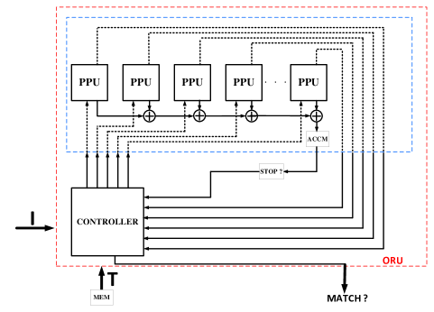
Figure 1: This is a circuit diagram for our computational algorithm in Section III-C. Such a system contains a cluster of simple primitive units - Patch Processing Units (PPUs), which take in $I|P_{i}$ and $t|N_{i}$ and return whether there was a match (if so, its contribution to the energy) or not, and whether to continue processing $P_{i}$ by splitting. Notice that once the accumulation of the energies emitted from the PPU’s (collected by the ACCM) is less than the threshold, processing is stopped (even though all patches are not processed) if it is only desired to know whether $I$ and $t$ correspond to the same scene. The controller manages the patches to process with the limited available number of PPU’s. Several of the ORU’s can be connected in parallel with the test image $I$ and the training templates $t_{1},\ldots,t_{m}$ accessed from memory for the primitive system discussed in Section III-D.

IV Discussion

IV-A Relation to 3D Reconstruction (Static Case)

One can think of our approach (in the special case of a static scene) as related to matching by attempting 3D reconstruction. The results of the structure from motion problem [18, 19] (i.e., in the case of a static scene not a dynamic one) indicate that (with suitable priors), the 3D geometry of the scene can be recovered, so the 3D scene is essentially coded in two images of the scene. Therefore, once the correct training template and the image to be recognized are associated, the 3D object is known (the part that is co-visible). Hence, it is clear that our mathematical framework and proposed procedure for recognition is equivalent to attempting 3D reconstruction, and determining whether the reconstruction has been successful (through threshold $T_{3}$), but reconstruction is not actually done. The 3D prior on scene is equivalent to a prior on the image-induced transformation, the prior is that coarse transformations are favored over finer transformations as our algorithm is a coarse to fine approach. This translates to a 3D prior that the scene is as flat whenever possible, but since fine transformations (i.e., small patch sizes) can also be used, the prior used is not a flat scene globally.

IV-B Relation to Existing Work

In [14], it is stated that nuisances must be eliminated at decision time (a point that is the basis of our approach), however, the reason stated in [14] for nuisances being eliminated at decision time is far different than our stated reasons of the tradeoff between invariance and discriminability. The reason given in [14] is “… for a nuisance, to be eliminated in pre-processing without loss of discriminative power, it should be invertible and commutative [w.r.t. non-invertible nuisances, i.e., noise, quantization, or occlusion],” suggesting that pre-processing should be avoided because of the non-invertible nuisances. Our results state that no pre-processing should be done to eliminate nuisances. For the case of viewpoint, the effects of viewpoint cannot be removed in a pre-processing step without inevitably losing discriminability (even without interaction by non-invertible nuisances); eliminating viewpoint may only done with knowledge of the second image, not in a pre-processing step. Further, our mathematical framework and computational algorithm are completely different. Also, the work in [14] applies to tracking (small deformations), but our algorithm is built for large deformations and motion.

IV-C Comment on Real Physical Systems

Our analysis and mathematical framework are done in the continuum, i.e., we haven’t addressed the nuisances of quantization (both in time and space) and noise, that are present in real systems. In the continuum, our results state that the best approach to determine the right level of invariance and discriminability is to determine that when the test image (acquired at infinite resolution) is available and is being matched to the stored infinite dimensional representation of the training image. One may argue that this is too idealistic, and that the issue that one should address is how to find the right tradeoff between how much (and what) of the test image and training image to throw away such that the recognition system makes the least error. In this regard, the work of [14] is interesting, which looks into this question. We agree with that approach, however, it is surely important to analyze the idealistic case as it provides the limits as to how the discriminability/invariance issue is addressed as the computational and memory resources are increased.

V Experiments

In this section, we demonstrate our algorithm working on establishing correspondence of two images from the same scene. We are interested in establishing correspondence of images taken from dynamic 3D scenes with camera viewpoint change, 3D object deformations, occlusions, and close up shots (so that there are significant changes of shape in the 2D images, and the time between frames is large so trackers and optical flow methods would fail). To this end, we obtain corresponding images from closeups in sports video. As there is no methodology for testing ground truth (e.g., epipolar geometry doesn’t apply to deforming objects), we verify matches manually (and this cannot be done on large-scale unfortunately). Figure 2 shows the decisions that our algorithm has made to establish matches, and the final matching on a sample image. Note for all experiments, we choose $\lambda_{1}=\lambda_{2}$ (i.e., only uniform scalings) for simplicity and speed.

Although our main contribution is a methodology for how to design a feature exhibiting the right tradeoff between invariance and discriminability, which leads to a joint feature extraction and matching framework, we show comparison to feature-based matching methods. We are not trying to prove that we out-perform every method, but simply try to give some idea how our algorithm compares to methods that do not setup the problem jointly. In all the experiments, we have spent much time tuning the parameters of SIFT (indeed, we have run SIFT on many different parameter configurations using the VLFeat [20] implementation, and show the best results). We also compare to Harris-Affine with a SIFT descriptor, and online code was used that did not allow for changing parameters [21] (we tried many different combinations of detectors and descriptors, but the combination of Harris-Affine and a SIFT descriptor, and the SIFT [2] were best). Figure 3 shows the results. First, we show our algorithm working on the Graffiti Dataset (where classical methods apply as the scene is flat). Our method gives comparable results on these images. Note that for very large perspective change, our current implementation of affine transforms on patches is not sufficient (although it is straight forward to add perspective to our model).

In the next images of Figure 3, we show only the foreground feature matches as we want to test our algorithm on 3D deformations and viewpoint change for non-flat scenes. Again, we have exhaustively searched over all parameters of SIFT and displayed the best results. It can be seen that the proposed method captures much more of the foreground area than SIFT and Harris-Affine, and makes few mistakes.

A quantitative assessment is given in Figure 4 using standard evaluation metrics, accuracy and repeatability. For standard feature matching methods, these are computed as follows:

$$\mbox{repeatability}=\frac{\mbox{\# features matched}}{\mbox{min \# of features detected in $I_{1}$ and $I_{2}$}},\,\,\mbox{accuracy}=\frac{\mbox{\# correct matches}}{\mbox{\# features matched}}.$$ (9)

The proposed method mostly performs better. Note that in the computation of repeatability for our method, we use the number of patches that were considered as the denominator in the above formula, others remain the same. In Figure 4, the $x-$axis in the bar graphs indicate the image number in the same ordering as the images stacked in Figure 3 on the left column. We wish to point out that it may be the case that the standard evaluation metrics do not capture the full benefit of our method, as can be seen in Figure 3: in contrast to other feature-based matching techniques, our method captures almost the whole region of the foreground (minus occlusion) and most matches are correct whereas the other approaches cover very little of the foreground area.

Figure 2: This figure illustrates our method working. Top left: $I_{1}$ with the patches that were processed in our algorithm (i.e., either matched or rejected due to being not discriminative enough) superimposed. Top right: $I_{1}$ and $I_{2}$. Bottom left: the decisions that were made in the algorithm (i.e., red-matched, blue - rejected for non-discriminability, black - rejected for being too small). Bottom right: matching patches. It is interesting to see that most processing is happening near occlusions, as expected.

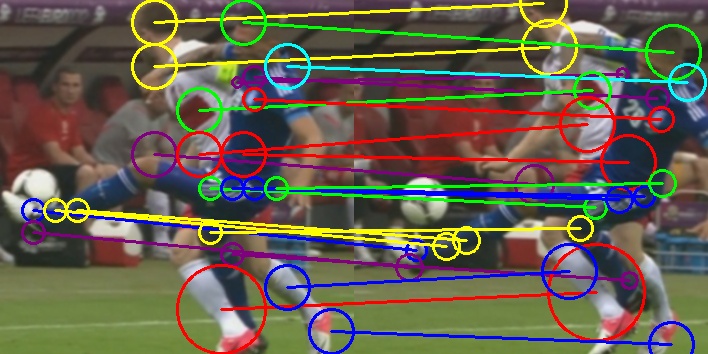
Figure 3: Left column: $I_{1}$ and $I_{2}$, second column: results of the proposed method, third column: results of SIFT [2], and fourth column: results of Harris-Affine detector [3] and a SIFT descriptor.

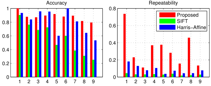
Figure 4: This figure shows quantitative comparison of the proposed method to standard methods, SIFT and Harris Affine (with a SIFT descriptor) using standard metrics - repeatability and accuracy. Our method yields higher repeatability, and many times higher accuracy (Harris affine achieves high accuracy by matching only a few features). The proposed method is a different paradigm than current feature-based matching, and so standard evaluation metrics may be insufficient to illustrate the power of our method.

VI Conclusion

We have addressed the question of how to construct features in a way that has the correct tradeoff between invariance and discriminability. We showed that the question can only be answered at match time. In otherwords, we have shown that the right level of invariance versus discriminability cannot be determined in a pre-processing step (without additional information of the 3D scene). This has led us to a joint problem of feature extraction and matching. We have created an effective computational algorithm. Our algorithm is designed for matching under large 3D object deformation, camera viewpoint change, and occlusions. We have illustrated our method on images from the same scene that exhibit the aforementioned phenomena, and showed some comparison to standard feature based methods where feature computation is done in a pre-processing step. Experiments suggest that our method is more effective in the case of large 3D deformation, and camera viewpoint for non-planar scenes.

References

- [1] U. Grenander, Elements of pattern theory. Johns Hopkins University Press, 1996.
- [2] D. Lowe, “Distinctive image features from scale-invariant keypoints,” International journal of computer vision, vol. 60, no. 2, pp. 91–110, 2004.
- [3] K. Mikolajczyk and C. Schmid, “Scale & affine invariant interest point detectors,” International journal of computer vision, vol. 60, no. 1, pp. 63–86, 2004.
- [4] J. Matas, O. Chum, M. Urban, and T. Pajdla, “Robust wide-baseline stereo from maximally stable extremal regions,” Image and Vision Computing, vol. 22, no. 10, pp. 761–767, 2004.
- [5] B. Horn and B. Schunck, “Determining optical flow,” Artificial intelligence, vol. 17, no. 1, pp. 185–203, 1981.
- [6] M. Beg, M. Miller, A. Trouvé, and L. Younes, “Computing large deformation metric mappings via geodesic flows of diffeomorphisms,” International Journal of Computer Vision, vol. 61, no. 2, pp. 139–157, 2005.
- [7] J. Burns, R. Weiss, and E. Riseman, “The non-existence of general-case view-invariants,” Geometric invariance in computer vision, vol. 1, pp. 554–559, 1992.
- [8] H. Chen, P. Belhumeur, and D. Jacobs, “In search of illumination invariants,” in Computer Vision and Pattern Recognition, 2000. Proceedings. IEEE Conference on, vol. 1. IEEE, 2000, pp. 254–261.
- [9] G. Sundaramoorthi, P. Petersen, V. Varadarajan, and S. Soatto, “On the set of images modulo viewpoint and contrast changes,” in Computer Vision and Pattern Recognition, 2009. CVPR 2009. IEEE Conference on. IEEE, 2009, pp. 832–839.
- [10] T. Poggio, “The computational magic of the ventral stream,” Nature Precedings, 2011.
- [11] S. Mallat, “Group invariant scattering,” Communications on Pure and Applied Mathematics, vol. 65, no. 10, pp. 1331–1398, 2012.
- [12] S. Soatto, “Actionable information in vision,” in Computer Vision, 2009 IEEE 12th International Conference on. IEEE, 2009, pp. 2138–2145.
- [13] T. Cover and J. Thomas, Elements of information theory. Wiley-interscience, 2006.
- [14] T. Lee and S. Soatto, “Video-based descriptors for object recognition,” Image and Vision Computing, vol. 29, no. 10, pp. 639–652, September 2011.
- [15] D. Mumford and J. Shah, “Boundary detection by minimizing functionals,” in Proc. IEEE Conference on Computer Vision and Pattern Recognition, San Francisco, CA, 1985.
- [16] T. Brox, C. Bregler, and J. Malik, “Large displacement optical flow,” in Computer Vision and Pattern Recognition, 2009. CVPR 2009. IEEE, 2009, pp. 41–48.
- [17] D. Cremers and S. Soatto, “Motion competition: A variational approach to piecewise parametric motion segmentation,” International Journal of Computer Vision, vol. 62, no. 3, pp. 249–265, 2005.
- [18] A. J. Yezzi and S. Soatto, “Structure from motion for scenes without features,” in Proceedings of the IEEE Conference on Computer Vision and Pattern Recognition, vol. 1, June 2003, pp. 525–532.
- [19] R. Hartley and A. Zisserman, Multiple view geometry in computer vision. Cambridge Univ Press, 2000, vol. 2.
- [20] A. Vedaldi and B. Fulkerson, “Vlfeat: An open and portable library of computer vision algorithms,” in Proceedings of the international conference on Multimedia. ACM, 2010, pp. 1469–1472.
- [21] K. Mikolajczyk and C. Schmid, “A performance evaluation of local descriptors,” Pattern Analysis and Machine Intelligence, IEEE Transactions on, vol. 27, no. 10, pp. 1615–1630, 2005.