Abstract

We present a general construction for dependent random measures based on thinning Poisson processes on an augmented space. The framework is not restricted to dependent versions of a specific nonparametric model, but can be applied to all models that can be represented using completely random measures. Several existing dependent random measures can be seen as specific cases of this framework. Interesting properties of the resulting measures are derived and the efficacy of the framework is demonstrated by constructing a covariate-dependent latent feature model and topic model that obtain superior predictive performance.

1 Introduction

Motivated by a desire for flexible models that minimize assumptions about the underlying structure of our data, Bayesian nonparametric models have garnered much attention in the machine learning and statistics communities. Most Bayesian nonparametric models assume observations are exchangeable. In real life, this assumption is usually hard to justify. We often have side information – for example time stamps or geographical location – that we believe influences the latent structure of our data.

There has been growing interest in models that challenge this exchangeability assumption, while still maintaining desirable properties of the original nonparametric processes. A dependent nonparametric process (MacEachern, 1999) is defined as a distribution over collections of measures indexed by values in some covariate space, such that the marginal distribution at some covariate value is described by a known nonparametric process. A number of authors have proposed dependent versions of the Dirichlet process (for example Griffin & Steel, 2006; Rao & Teh, 2009; Chung & Dunson, 2011; Duan et al., 2007; Caron et al., 2007), the Pitman-Yor process (Sudderth & Jordan, 2009) and the Indian buffet process (Ren et al., 2011; Williamson et al., 2010; Zhou et al., 2011).

Most of the basic nonparametric processes found in the literature can be formulated in terms of completely random measures (CRMs, Kingman, 1967) – distributions over measures that assign independent masses to disjoint subsets of the space on which they are defined. For example, the Dirichlet process can be obtained by normalizing the CRM known as the gamma process. The IBP can be described in terms of a mixture of Bernoulli processes, where the mixing measure is a completely random measure known as the beta process (Thibaux & Jordan, 2007).

Completely random measures on some space $\Theta$ can be represented as Poisson processes on the product space $\Theta\times\mathbb{R}^{+}$. In this paper, we show that a large class of dependent nonparametric processes can be described in terms of operations on Poisson processes on an augmented space $\mathcal{X}\times\Theta\times\mathbb{R}^{+}$. This framework offers great flexibility in the form of the dependency, and often leads to simple posterior updates, as any conjugacy present in the non-dependent version of the model is carried over to the dependent case. The resulting class of distributions contains, or is related to, several existing models, such as the kernel beta process (Ren et al., 2011) and the spatial normalized gamma process (Rao & Teh, 2009). A major contribution of this paper is to express the relationships between these models in a simple manner, and aid in the understanding of existing models and the development of new models and inference techniques.

We use this framework as a basis for two models: a covariate-dependent latent variable model based on the beta process, and a covariate-dependent topic model based on the gamma process. We show that incorporating dependency can improve the predictive power of Bayesian nonparametric models, and that by making use of conjugacy and simpler forms of dependence, we can obtain comparable results to existing dependent nonparametric processes, with a dramatic decrease in time spent on inference.

2 Background

A completely random measure (CRM) is a distribution over measures on some measurable space $(\Theta,\mathcal{F}_{\Theta})$, such that the masses $\Gamma(A_{1}),\Gamma(A_{2}),\dots$ assigned to disjoint subsets $A_{1},A_{2},\dots\in\mathcal{F}_{\Theta}$ by a random measure $\Gamma$ are independent (Kingman, 1967). The class of completely random measures contains important distributions such as the beta process, the gamma process, the Poisson process and the stable subordinator.

A CRM on $\Theta$ is characterized by a positive Lévy measure $\nu(d\theta,d\pi)$ on the product space $\Theta\times\mathbb{R}^{+}$, and can be represented in terms of a Poisson process on this space. Let $\Pi=\{(\theta_{k},\pi_{k})\}_{k=1}^{\infty}$ be a Poisson process on $\Theta\times\mathbb{R}^{+}$, with mean measure $\nu(d\theta,d\pi)$. Then the completely random measure with Lévy measure $\nu(d\theta,d\pi)$ can be represented as $\Gamma=\sum_{k=1}^{\infty}\pi_{k}\delta_{(\theta_{k})}$.

De Finetti’s theorem tells us that any infinitely exchangeable sequence can be described as a mixture of i.i.d. distributions. CRMs provide the mixing distribution in the de Finetti representation of a number of useful exchangeable distributions. For example, we can represent the Indian buffet process, a distribution over exchangeable binary matrices, as a beta process mixture over countably infinite collections of Bernoulli random variables (Thibaux & Jordan, 2007). The resulting distribution over exchangeable binary matrices is an appropriate prior for nonparametric versions of latent feature models. Other distributions over exchangeable matrices have been defined using the beta process (Zhou et al., 2012b) and the gamma process (Titsias, 2007; Saeedi & Bouchard-Côté, 2011) as mixing measures.

We are often interested in learning distributions over probability distributions – for example, for use in clustering or density estimation. Two important examples of such distributions – the Dirichlet process and the normalized stable process – can be obtained by normalizing the gamma process and the stable subordinator, respectively. CRMs can also be used directly as a prior on hazard functions in survival analysis applications (Ibrahim et al., 2005).

3 Construction of dependent random measures via thinned Poisson processes

Let $\Pi=\{(x_{i},\theta_{i},\pi_{i})\}_{i=1}^{\infty}$ be a Poisson process (PP) on the space $\mathcal{X}\times\Theta\times\mathbb{R}^{+}$. This space has three components: $\mathcal{X}$, an auxiliary space; $\Theta$, a space of parameter values; and $\mathbb{R}^{+}$, which will be the masses making up the random measures. Let the mean measure of $\Pi$ be described by the positive Lévy measure $\nu(dx,d\theta,d\pi)$. While the theory herein applies for any such Lévy measure, we will focus on the class of Lévy measures that factorize as

$$\textstyle\nu(dx,d\theta,d\pi)=G(dx,d\theta)\nu_{0}(d\pi).$$

This corresponds to the class of homogeneous completely random measures, where the size of an atom is independent of its locations in $\Theta$ and $\mathcal{X}$

It follows that $\Gamma=\sum_{k=1}^{\infty}\pi_{k}\delta_{(x_{k},\theta_{k})}$ is a CRM on $\mathcal{X}\times\Theta$. By the mapping theorem of PPs (Kingman, 1993) we see that $B=\sum_{k=1}^{\infty}\pi_{k}\delta_{\theta_{k}}$ is a CRM on $\Theta$ with rate measure given by

$$\nu_{B}(d\theta,d\pi)=\int_{\mathcal{X}}\nu(dx,d\theta,d\pi)=\nu_{0}(d\pi)\int_{\mathcal{X}}G(dx,d\theta)$$

Let $\mathcal{T}$ be some covariate space – for example time – and let $\{p_{x}:\mathcal{T}\rightarrow[0,1]\}_{x\in\mathcal{X}}$ be a collection of functions indexed by $x\in\mathcal{X}$. We can now construct a family of random measures $B_{t}$ dependent on values $t\in\mathcal{T}$. For each point $(x_{k},\theta_{k},\pi_{k})\in\Pi$, define a collection $\{r_{k}^{t}\}_{t\in\mathcal{T}}$ of Bernoulli random variables (so $r^{t}_{k}$ is a binary valued random function on $\mathcal{T}$), such that $p(r^{t}_{k}=1)=p_{x_{k}}(t)$. The $r^{t}_{k}$s indicate whether atom $k$ in the global measure $B$ appears in the local measure $B_{t}$ at covariate value $t$. Therefore, the function $p_{x}$ controls the degree of dependence between two measures $B_{t}$ and $B_{t^{\prime}}$.

Appealing to the marking theorem of PPs (Kingman, 1993), we see that the resulting thinned PP $\Pi_{t}$ and its associated rate measure $\nu_{t}$ are described by

$$\Pi_{t} =\left\{(x_{k},\theta_{k},\pi_{k})\;|\;r^{t}_{k}=1\right\}_{k=1}^{\infty}$$

$$\nu_{t}(A,d\theta,d\pi) =\int_{x\in A}p_{x}(t)\nu(dx,d\theta,d\pi)$$

for $A\in\mathcal{F}_{\mathcal{X}}$. Then, applying the mapping theorem to $\Pi_{t}$ and employing the sum form of a CRM, we find

$$\textstyle B_{t}=\sum_{k\;:\;r^{t}_{k}=1}\pi_{k}\delta_{\theta_{k}}=\sum_{k=1}^{\infty}r^{t}_{k}\pi_{k}\delta_{\theta_{k}}$$

is a CRM on $\Theta$ that varies with $t\in\mathcal{T}$ and has rate measure

$$\nu_{B_{t}}(d\theta,d\pi)=\int_{\mathcal{X}}p_{x}(t)\nu(dx,d\theta,d\pi)=\nu_{t}(\mathcal{X},d\theta,d\pi)$$ (1)

which, given certain forms of $p_{x}$ and $\nu$, may be simplified further. We refer to $\{B_{t}\}_{t\in\mathcal{T}}$ as a thinned CRM.

If the thinning function $p_{x}(t)$ is taken to be a bounded unimodal kernel function $K(t,m,\phi)$, where $x:=(m,\phi)$ gives the center and dispersion of the kernel, we can interpret the model as saying that each atom $\pi_{k}\delta_{(x_{k},\theta_{k})}$ of the CRM defined on $\mathcal{X}\times\Theta\times\mathbb{R}^{+}$ is “active” in some subregion of $\mathcal{T}$, dictated by a location $m_{k}$ and a dispersion $\phi_{k}$. However, $p_{x}$ need not be unimodal, or even a kernel. Later, we will consider a form for $p_{x}$ that allows atoms to be active at multiple locations.

3.1 Properties of thinned CRMs

The moments of $B_{t}(A)$ for any $x\in\mathcal{X}$ and $A\in\mathcal{F}_{\Theta}$ can be determined from Campbell’s theorem (Kingman, 1993) using Eq. 1. Another quantity of interest is the correlation between the marginals of a thinned CRM at two covariate values $t$ and $t^{\prime}$. Assuming that $\mathbb{V}(\pi_{k})<\infty$, which holds for most CRMs used in practice, we have

$$\text{Corr}(B_{t}(A),B_{t^{\prime}}(A))$$

$$=\frac{\displaystyle\sum_{k:\theta_{k}\in A}\mathbb{E}(r^{t}_{k}r^{t^{\prime}}_{k}|p^{t},p^{t^{\prime}})\mathbb{V}(\pi_{k})}{\sqrt{\displaystyle\sum_{k:\theta_{k}\in A}\mathbb{E}((r^{t}_{k})^{2})\mathbb{V}(\pi_{k})\displaystyle\sum_{k:\theta_{k}\in A}\mathbb{E}((r^{t^{\prime}}_{k})^{2})\mathbb{V}(\pi_{k})}}$$

$$=\frac{<p^{t},p^{t^{\prime}}>}{\left|\left|p^{t}\right|\right|\left|\left|p^{t^{\prime}}\right|\right|}\,$$

where $p^{t}=(p_{x_{k}}(t))_{k=1}^{\infty}$. In other words, the correlation between the two random measures is given by the correlation between the thinning indicators $r^{t}$ and $r^{t^{\prime}}$, and is independent of the Lévy measure. We can therefore specify the correlation between the measures at different covariate values through the form of $p_{x}$. In general, smooth functions will capture the intuitive notion that measures at nearby covariates should use a similar set of atoms. Arbitrary correlation structures can be obtained via appropriate choice of $p_{x}$.

A key property of the construction is that the resulting dependent random measures are of the same form as the original process – the component $\nu_{0}$ of the Lévy measure that governs the atom sizes is unchanged, and the $\pi_{k}$s are distributed as before. This is desirable in order to retain conjugacy in the model being used. The thinned CRM framework puts very few restrictions on the original process allowing us to construct a large family of dependent CRMs, whereas previous constructions have been limited to specific processes.

4 Examples

In this section, we describe thinned CRMs with two different dependency structures, and two hierarchical models based on such thinned CRMs.

4.1 A single-location thinned CRM

One of the simplest forms of covariate dependency is to assume that the expected correlation between two measures decreases with increasing distance in covariate space. This can be captured by choosing the thinning probability for each atom of the global CRM to be a unimodal distribution centered on a point in covariate space – as we move away from this location in covariate space, the probability of a covariate-dependent measure featuring this atom will decrease monotonically. Such a model is described as:

$$\textstyle\Gamma:=\sum_{k=1}^{\infty}\pi_{k}\delta_{(x_{k},\theta_{k})} \sim\text{CRM}(\nu(dx,d\theta,d\pi))$$ (2)

$$\textstyle p_{x}(t) =f(|x-t|)$$

$$\textstyle r_{k}^{t} \sim\text{Ber}(p_{x_{k}}(t))$$

$$\textstyle B_{t} :=\textstyle{\sum_{k=1}^{\infty}}r_{k}^{t}\pi_{k}\delta_{\theta_{k}}\,,$$

where $\mathcal{X}=\mathcal{T}$ and $f:\mathcal{X}\rightarrow[0,1]$ is some unimodal function on $\mathcal{X}$, for example a scaled Gaussian density.

4.2 A multiple-location thinned CRM

The form of dependency in Section 4.1 is restrictive: the probability of an atom contributing to a CRM decays with distance in covariate space. If each atom corresponds to a feature in a latent factor model, this means that, in practice, each feature is only going to contribute to data points within a restricted covariate range.

Greater flexibility can be obtained by replacing the unimodal function $f$ in Eq. 2 with an arbitrary function $g$. The function $g$ might, for example, be a Gaussian random field on $\mathcal{T}$ that has been transformed via a sigmoid function at every value of $t\in\mathcal{T}$.

As a concrete example, consider one such construction of a covariate-dependent beta process. Here, the base CRM is a homogeneous beta process, with Lévy measure $\nu_{B}(dx,d\theta,d\pi)=cH(dx)B_{0}(d\theta)\pi^{-1}(1-\pi)^{c-1}d\pi$ on $\mathcal{X}\times\Theta\times[0,1]$, for some constant $c>0$ and probability measures $H$ and $B_{0}$.

For the thinning function, we choose a transformed relevance vector machine kernel. The relevance vector machine (Tipping, 2001) can be seen as the weighted sum of (a finite number of) Gaussian kernels. Locations in the auxiliary space $\mathcal{X}$ correspond to the set of centers, weights and widths of these kernels. A standard modeling decision, which we adopt in our experiments, is to fix the centers of these kernels to the $L$ locations $t_{1},\dots,t_{L}$ of the data in covariate space $\mathcal{T}$. Each location $x_{k}\in\mathcal{X}$ therefore corresponds to a set of $L+1$ weights $\omega_{lk}\in\mathbb{R}$, and a (shared) width $\phi_{k}$ selected from a fixed dictionary $D$. Our auxiliary space is therefore defined as $\mathcal{X}:=\mathbb{R}^{L+1}\times D$, and our base measure $H(dx)$ can be decomposed into a normal-inverse Gamma prior on each of the weights, and a categorical prior on the widths. In our experiments, we chose small values of $c_{0}$ and $d_{0}$ (see below) resulting in most $\omega_{lk}$ being small, which implies that $p_{x_{k}}(t)$ will be large at few locations.

In order to ensure valid thinning probabilities, we transform the RVM kernel pointwise using a probit function. The generative procedure is given by:

$$\begin{split}\Gamma&:=\textstyle{\sum_{k=1}^{\infty}}\pi_{k}\delta_{(x_{k},\theta_{k})}\sim\text{CRM}(\nu_{B}(dx,d\theta,d\pi))\\ \omega_{lk}&\sim\text{NiG}(0,c_{0},d_{0}),\;\phi_{k}\sim\text{Cat}(\phi_{1},\ldots,\phi_{D})\\ p_{x_{k}}(t)&=\Phi\big{(}\omega_{0k}+\textstyle{\sum_{l=1}^{L}}\omega_{lk}\exp(-\phi_{k}\left|\left|t-t_{l}\right|\right|_{2}^{2})\big{)}\\ \textstyle r_{k}^{t}&\sim\text{Ber}(p_{x_{k}}(t))\\ \textstyle B_{t}&:=\textstyle{\sum_{k=1}^{\infty}}r_{k}^{t}\pi_{k}\delta_{\theta_{k}}\,.\end{split}$$ (3)

4.3 A dependent latent feature model

We can use covariate-dependent CRMs to construct covariate-dependent latent variable models. In such a setting, each atom of the CRM on $\mathcal{X}\times\Theta\times\mathbb{R}^{+}$ is associated with a latent feature, and the mass of that atom parameterizes a distribution over the weight assigned to that feature. Each data point then selects a weight for each feature according to the masses of the atom in the corresponding thinned CRM.

As an example, consider a latent feature model based on the covariate-dependent beta process described in Eq. 3, where $B_{0}(d\theta)$ is the multivariate Gaussian prior measure – i.e. each latent feature is a real-valued vector. For each covariate value $t\in\mathcal{T}$, a subset of these features, and their corresponding atom weights $\pi_{k}$, are selected as in Eq. 3 to give a local measure $B_{t}=\sum_{k=1}^{\infty}r_{k}^{t}\pi_{k}\delta_{\theta_{k}}$. For each data point $n$ at covariate value $x$, a subset of features are chosen by selecting each feature with probability $r_{k}^{t}\pi_{k}$. The selected features are combined via linear superposition, and Gaussian noise is added. The generative model is as follows:

$$z_{k}^{n,t} \sim\text{Ber}(r_{k}^{t}\pi_{k})\;,t\in\mathcal{T},k\in\mathbb{N},n\in\{1,\dots,N_{t}\}$$

$$A_{k} \sim\mathcal{N}(0,\sigma_{A}^{2}\text{I})\;,k\in\mathbb{N}$$

$$y^{n,t} \sim\mathcal{N}(\textstyle\sum_{k}z_{k}^{n,t}A_{k},\sigma^{2}\text{I}),$$

where $r_{k}^{t}$ and $\pi_{k}$ are sampled according to Eq. 3 and $N_{t}$ denotes the number of data points with covariate $t$. In the case where each observation is associated with a unique covariate we simplify the notation to $z_{nk}$ and $r_{nk}$.

This model is a dependent version of the linear Gaussian IBP model proposed by Griffiths & Ghahramani (2005). The model can be extended by using different models for generating and combining the features (Wood et al., 2006; Miller, 2011), or by sampling a real-valued weight $s_{k}^{n,t}$ for each instance of a feature and combining them as $y^{n,t}\sim\mathcal{N}(\sum_{k}s^{n,t}z_{k}^{n,t}A_{k},\sigma^{2}\text{I})$ (Zhou et al., 2012a).

4.4 A time-varying topic model

Topic models are popular latent variable models that decompose a text corpus into the underlying topics. Topic models define a topic as a probability distribution over a finite vocabulary with $P$ terms. The simplest topic model is latent Dirichlet allocation (LDA, Blei et al., 2003) where the words in each document are generated by first drawing which topic the word exhibits from a document-specific topic distribution and then drawing the actual word from the corresponding topic. The basic LDA model has been extended in many ways, for example, to allow correlated topics (Blei & Lafferty, 2007; Paisley et al., 2011), to allow the topics to drift over time (Blei & Lafferty, 2006; Wang et al., 2008) and to allow topic usage to vary over time (Wang & McCallum, 2006).

The thinned CRM construction described in this paper can be used to construct a time-varying topic model where the topics are assumed fixed, but the usage of the topics changes over time. This assumption allows the learned topics to be localized in time. As in Zhou et al. (2012b), we formulate our topic model as a Poisson factor model.

We use a thinned gamma process (tGaP) to model the global popularity of each topic and the relevance vector machine in Eq. 3 as the thinning function. Let $w_{pnt}$ denote the number of times the $p$th word (in a vocabulary of $P$ words) appears in the $n$th document at time $t$. Let $\nu_{G}(dx,d\theta,d\pi)=\nu_{G0}(d\pi)H(dx)B_{0}(d\theta)$, where $\nu_{G0}(d\pi)=\gamma\pi^{-1}\exp(-\lambda\pi)d\pi)$ is the Lévy measure of the gamma process; $B_{0}(d\theta)$ is the $P$-dimensional Dirichlet distribution with parameter $\alpha_{\theta}$; and $H(dx)$ is the prior over parameters for the RVM as described in Section 4.2.

The complete model, denoted tGaP-PFA, is specified as

$$\Gamma :=\sum_{k=1}^{\infty}\pi_{k}\delta_{(x_{k},\theta_{k})}\sim\mbox{CRM}(\nu_{G}(dx,d\theta,d\pi))$$ (4)

$$p_{x_{k}}(t) =\Phi\big{(}\omega_{0k}+\textstyle{\sum_{l=1}^{L}}\omega_{lk}\exp(-\phi_{k}\left|\left|t-t_{l}\right|\right|_{2}^{2})\big{)}$$

$$\textstyle r_{k}^{n,t} \sim\text{Ber}(p_{x_{k}}(t))$$

$$\textstyle G_{n,t} :=\textstyle{\sum_{k=1}^{\infty}}r_{k}^{n,t}\pi_{k}\delta_{\theta_{k}}$$

$$\beta_{k}^{n,t} \sim\text{Ga}(e,1),n=1,\dots,N_{t},k\in\mathbb{N}$$

$$\tilde{w}_{pntk} \sim\text{Pois}(\theta_{kp}r_{k}^{n,t}\pi_{k}\beta_{k}^{n,t})$$

$$w_{pnt} =\sum_{k=1}^{\infty}\tilde{w}_{pntk}\sim\text{Pois}(\sum_{k=1}^{\infty}\theta_{kp}r_{k}^{n,t}\pi_{k}\beta_{k}^{n,t})$$

where the RVM machinery is presented in Eq. 3. The vectors $\theta_{k}=(\theta_{k1},\dots,\theta_{kP})$ are the topics, the atom sizes $\pi_{k}$ can be interpreted as the baseline rate that this topic generates words and the $\beta_{k}^{n,t}$ are document-specific modulations of the global rate so that documents can exhibit a topic more or less than the baseline.

5 Relationship with other processes

The framework for dependent random measures proposed in Section 3 is very general, and includes or is related to a number of existing models, as we describe below.

5.1 Kernel beta process

The kernel beta process (KBP, Ren et al., 2011) has an interesting interpretation in terms of thinned CRMs. Let $\mathcal{T}$ be our covariate space, $\Psi$ be a space of possible dispersions, and define our auxiliary space as $\mathcal{X}:=\mathcal{T}\times\Psi$. Let $\nu(dx,d\theta,d\pi):=\nu_{0}(d\pi)H(dx)B_{0}(d\theta)$ be a Lévy measure on $\mathcal{X}\times\Theta\times\mathbb{R}^{+}$, such that $\nu_{0}(d\pi)=c\pi^{-1}(1-\pi)^{c-1}d\pi$. Let $p_{x}(t)=K(t,m,\psi)$ for every $x:=m\times\psi\in\mathcal{X}$, where $K(\cdot,\cdot,\cdot)$ is a unimodal kernel with mean $m$ and dispersion $\psi$ bounded above by $1$. Then, the expectation of a realization of the corresponding thinned CRM is given by

$$\mathbb{E}_{p_{x}}[B_{t}]=\sum_{k=1}^{\infty}\mathbb{E}_{p_{x}}[r_{k}^{t}]\pi_{k}\delta_{\theta_{k}}=\sum_{k=1}^{\infty}K(t,m_{k},\psi_{k})\pi_{k}\delta_{\theta_{k}}\,,$$

which is exactly the form of the KBP. In other words, the KBP is a mixture of kernel-thinned beta processes. The thinned beta process provides a generative process for the KBP, which could be useful for formulating the KBP in a probabilistic programming language (e.g. Goodman et al., 2008). In fact, the inference algorithm described in Ren et al. (2011) uses such a representation.

While the KBP can be described without using a thinned Poisson process representation, we feel that the above derivation is easier to interpret, and properties of the KBP can be simply derived by appealing to well-known properties of marked Poisson processes. Additionally, the thinned Poisson process construction makes extending the KBP idea to arbitrary CRMs simple, whereas the original construction relied on specific properties of the beta process.

5.2 Spatial normalized gamma processes

Just as a Dirichlet process can be constructed by normalizing a gamma process, a dependent Dirichlet process can be constructed by normalizing a thinned gamma process. If $\mathcal{X}=\mathcal{T}$ and the thinning probability is given by $p_{x_{k}}(t)=\int_{0}^{\infty}\mathbb{I}[|t-x_{k}|\leq\ell]f(\ell)d\ell$ for some distribution $f(\cdot)$ over window size $l$, then after normalization, this describes the spatial normalized Gamma processes (SN$\Gamma$P) of Rao & Teh (2009) where a Dirichlet process, $D_{t}$ exists at all covariate values.

Incorporating the Poisson process representation into the SN$\Gamma$P model could yield a number of benefits. The inference scheme described by Rao & Teh (2009) involves representing each $D_{t}$ as a mixture of independent DPs, and performing inference in the corresponding mixture of urn schemes. However, this approach does not scale well to higher dimensional covariate spaces, as the number of independent regions, and thus the number of DPs that need to be represented, grows exponentially with the dimensionality of the space. In addition, a naive MCMC implementation mixes poorly, necessitating the use of expensive split/merge Metropolis Hastings steps. Representing the SN$\Gamma$P as a normalized thinned CRM opens up the possibility of different inference algorithms that represent $D_{t}$ explicitly, and may yield more scalable and efficient implementations.

In addition, understanding the model in terms of thinned Poisson processes makes it easier to change the form of dependency from the box kernel employed in the original paper. Alternative kernels, for example an exponential kernel, could be used to give a softer falloff and hence more flexible dependency.

5.3 Ornstein-Uhlenbeck Dirichlet process

The Ornstein-Uhlenbeck Dirichlet process (OUDP, Griffin, 2007) can be constructed in a similar manner to the KBP, with an added normalization step. We define $\mathcal{T}=\mathbb{R}$ and $\mathcal{X}:=\mathbb{R}\times\Psi$, and let $\nu(dx,d\theta,d\pi):=\nu_{0}(d\pi)H(dx)B_{0}(d\theta)$ be a Lévy measure on $\mathcal{X}\times\Theta\times\mathbb{R}^{+}$ and $\Gamma$ the associated CRM. Let $\{G_{t}\}$ be the dependent CRM obtained when we choose the thinning probability $p_{x_{k}}(t)=K(t,m_{k},\psi_{k})$ to be an Ornstein-Uhlenbeck kernel, and $\nu_{0}(d\pi)$ to be the Lévy measure of a Gamma process. The OUDP is then obtained as $D_{t}(A)=\frac{\mathbb{E}_{p_{x}}[G_{t}(A)]}{\mathbb{E}_{p_{x}}[G_{t}(\Theta)]}$. For the Ornstein-Uhlenbeck kernel, Griffin showed that $D_{t}$ is a DP. Unfortunately, the proof does not easily extend to arbitrary kernels or higher dimensional spaces. However, treating $D_{t}$ as a mixture of normalized thinned CRMs immediately shows that if we instead consider the “complete representation” of the random measures $\{D_{t}\}_{t\in\mathcal{T}}$, then the marginal distributions are Dirichlet processes, regardless of what kernel we pick and the covariate space.

5.4 Other dependent nonparametric processes with Poisson process interpretations

In addition to models that can be represented in terms of thinned Poisson processes on an augmented space, there are a number of other models that can be described in terms of Poisson processes. Lin et al. (2010) create a Markov chain $P_{1},P_{2},\dots$ of Poisson processes on $\Theta\times\mathbb{R}^{+}$ such that, at each time point, the corresponding Poisson process is obtained by thinning the previous Poisson process and superimposing an independent Poisson process. The resulting chain of Poisson processes defines a Markov chain of gamma processes, which are normalized to give a Markov chain of Dirichlet processes. A similar procedure, with thinning probability that depends on the atom sizes, underlies the size-biased deletion form of the dependent Poyla urn model of Caron et al. (2007). These models do not fit neatly into the framework described in this paper, and are restricted to Markovian dependency and discrete covariate spaces.

6 Experimental evaluation

We illustrate the effectiveness of using a thinned CRM to relax the assumption of exchangeability in nonparametric Bayesian modeling on both synthetic and real data. Specifically, we consider the approaches described in Sections 4.3 and 4.4, where a probit RVM thinned CRM is used as the basis for covariate-dependent binary latent feature models and covariate-dependent topic models, respectively. The experiments using binary latent feature models are performed to allow comparisons to existing work and to show that the proposed prior is indeed capturing the structure, and not the likelihood. The topic model experiments are intended to highlight the ease with which we can incorporate dependency into more complex hierarchical models, and demonstrate the performance gains such covariate dependency can yield.

6.1 Inference

Inference in the probit RVM model described in Section 4.2 is carried out using Gibbs sampling. We consider a truncated version of the beta process and gamma process for computational simplicity. In both cases, we select a truncation level $K$. To approximate the beta process, we draw $K$ atom sizes from a $\text{Beta}\left(\frac{1}{K},1-\frac{1}{K}\right)$ distribution. The resulting $K$-dimensional vector can be shown to converge to a draw from a beta process as $T\rightarrow\infty$ (Paisley & Carin, 2009). Similarly, to approximate the gamma process, we draw $K$ atom sizes from a $\text{Ga}(\frac{1}{K},1)$ distribution.

The weights $\{\omega_{lk}\}$ can be sampled using the method of Albert & Chib (1993) using the $r_{k}^{t}$ of Eq. 3 as observations. To allow conjugate updates for $\pi_{k}$ we introduce an auxiliary variable $b^{n,t}_{k}$ for each data point and feature such that $z^{n,t}_{k}=1$ iff $b^{n,t}_{k}=1$ and $r^{t}_{k}=1$. We then sample $(b^{n,t}_{k},r^{t}_{k})$ from their joint distribution, which can be enumerated since both variables are binary. A similar scheme was used in Ren et al. (2011). Lastly, we sample the kernel dispersion parameters $\phi_{k}$ from a fixed finite dictionary of possible values with a uniform prior over the possible values.

For the latent feature model described in Section 4.3, the remaining Gibbs sampling equations are all easily derived by conjugacy, and Zhou et al. (2012a) provides most of the required distributions. For the topic model described in Section 4.4, the Gibbs sampling equations for the remaining variables are described in the supplement.

6.2 Dependent binary latent feature model: Synthetic data

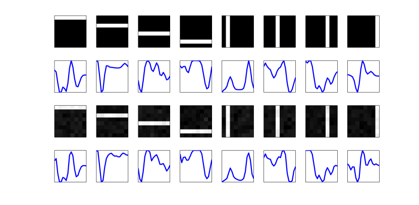
Figure 1: Recovering feature probabilities in synthetic data. Top row: Features used to generate synthetic data. Second row: Time-varying thinning probabilities used to generate synthetic data. Third row: Recovered features (manually aligned to match generating features). Bottom row: Recovered time-varying thinning probabilities.

To demonstrate the model’s ability to uncover covariate dependent structure we generated synthetic data similarly to the “bag of items” experiment in Williamson et al. (2010). Here, the covariate space is the real line, and the covariate values are the integers $1,\ldots,20$. The data was generated using eight 64-pixel image features (depicted in the top row of Fig. 1), and eight corresponding time-varying thinning probabilities generated using the RVM kernel described in Section 4.2, with kernel weights $\omega_{lk}\sim\kappa_{k}\delta_{0}+(1-\kappa_{k})\mathcal{N}(0,4)$, $\kappa_{k}\sim\text{Beta}\left(1,1\right)$. Each kernel had dispersion parameter $\phi$, implying that all features vary on the same scale. The resulting thinning probabilities $p_{x_{k}}(t)$ are shown in the second row of Fig. 1. For each location $t\in\{1,\ldots,20\}$ we generate a binary matrix $Z^{y}=\{z_{n,k}^{y}\}\in\{0,1\}^{100\times 8}$ of feature usage indicators for $100$ data points at location $y$ using the sampling equation for $z^{t}_{n,k}$ in Eq. 4.3. Finally, we generate data for each $t$ as $Y^{t}=Z^{t}A+E$, where the rows of $A$ are the eight features and $E$ is a matrix of observation noise with each entry normally distributed with mean $0$ and variance $0.25$.

We perform inference using the Gibbs sampler described above, with a truncation level of $20$ features and learned individual scales $\phi_{k}$ for each kernel. The resulting learned features and their respective thinning probabilities are depicted in the third and fourth rows of Fig. 1. The model usually learns the correct dimensionality of the data and thinning probabilities as in the case depicted, however, sometimes extra features are used to explain the noise present in the data in addition to the correct features.

6.3 Dependent binary latent feature model: U.N. development indicators

We evaluate the model in a predictive setting on a UN dataset consisting of 15 developmental indicators for 144 countries. This dataset was used by Williamson et al. (2010) to evaluate an alternative dependent latent feature model known as the dependent IBP (dIBP). The dIBP induces dependency directly between corresponding elements of a collection of binary vectors using a transformed Gaussian process.

We follow the experimental protocol used in Williamson et al. (2010) where 14 countries are selected at random as a test set, and the model is trained on the remaining 130 countries. For each test country we observe a single feature chosen at random (possibly a different feature for each country) and the goal is to predict the remaining 14 unobserved features. The covariate for the thinned beta process model is log-GDP of the country. We perform 10-fold cross-validation and report the mean RMSE and two standard deviations in Table 1 where we compare the results for an exchangeable beta-Bernoulli process feature model, the thinned beta process model and the dIBP model.

Table 1: RMSE on UN developmental data

Exchangeable	thinned BP	dIBP
$1.02\pm 0.08$	$0.85\pm 0.11$	$0.73\pm 0.05$

The thinned beta process model obtained lower RMSE than the exchangeable model on all folds, indicating that incorporating covariate information improves modeling performance. The best results are obtained by the dIBP. This is not surprising, because the Gaussian processes used are flexible enough to model arbitrary changes in the latent structure. However, this added performance comes at a cost – the dIBP uses a single Gaussian process for each latent feature, and inference in the Gaussian processes scales cubically with the number of covariate locations. In addition, the dIBP does not make use of conjugacy, which increases the computational costs. While the exchangeable model and the thinned BP models ran on the order of hours, the dIBP ran on the order of days. We feel the thinned BP provides a compromise between improved accuracy by taking covariate information into account and running time.

6.4 Time-varying topic model

We evaluate the time-dependent topic model proposed in Section 4.4 both quantitatively and qualitatively on the State of the Union dataset, which consists of the full texts of the addresses for presidents George Washington to George Bush covering the years 1780–2002. As in Wang & McCallum (2006) we break up the addresses into documents of three paragraphs. This resulted in 5997 documents. We created our vocabulary by computing the term-frequency inverse document frequency (TFIDF, Manning et al., 2008) score of all observed words and only keeping those with at least 10 occurrences in the corpus and in the upper 0.15 quantile of the observed TFIDF scores resulting in a vocabulary with 997 words. All results are reported for the Dirichlet parameter, $\alpha_{\theta}=0.05$, with comparable results obtained with other values. Large values of $\alpha_{\theta}$ result in few topics being learned and vice versa. We report the average number of topics learned for each model with with this setting of $\alpha_{\theta}$ in Table 2.

We evaluate our model using three tasks: perplexity on held out data; time-stamp prediction; and qualitative evaluation. The perplexity evaluation was carried out following Zhou et al. (2012b), by holding out $20\%$ of the words from each document, training the model on the remaining $80\%$ and computing the perplexity of the held-out words (as described in the supplement). We compared the tGaP-PFA model against a static version of the same model (obtained by deterministically setting all $r_{k}^{n,t}=1$) and against the beta-negative binomial process (BNBP) model of Zhou et al. (2012b).

The perplexity results are presented in Table 2. We see that the tGaP-PFA model obtains superior perplexity to the static version, showing that incorporating dependency can improve performance when the data is assumed to be non-exchangeable. The stationary version of the tGaP-PFA model is a much simpler model than the BNBP topic model, which unsurprisingly performs better. However, since the BNBP model is based on a stationary CRM, our results suggest that a dynamic version of the BNBP topic model, constructed with a thinned beta process, could achieve better performance than the stationary model.

Table 2: Average perplexity and average # of topics for State of the Union corpus over 5 hold-out sets.

	Static	Dynamic	BNBP
Perp.	$624.4\pm 2.0$	$528.6\pm 2.7$	$418.1\pm 0.9$
$\mathbb{E}[K]$	$5.4\pm 0.3$	$62.6\pm 0.8$	$198.4\pm 0.4$

We also evaluate the ability of the our dynamic model to predict the decade of a held-out document. We hold out $20\%$ of the documents in each decade and train the model on the remaining $80\%$. To predict the decade for a held-out document we find the decade that maximizes the predictive likelihood of the document. We compare the dynamic model with a static version where we train a separate static tGaP-PFA model at each timestamp and predict the decade of a held out document by choosing the decade with the maximum predictive likelihood. We also compare with a baseline prediction that selects a decade uniformly at random. The results are presented in Table 3 where we see that the dynamic model obtains $\approx 65\%$ reduction in absolute (L1) error and $\approx 4$X increase in accuracy over the static and baseline models. Interestingly the static model performs on par with the baseline indicating substantial over-fitting and displaying the necessity of taking time into account.

Table 3: Predicting the decade of documents reported as absolute (L1) error in decades and accuracy (average over 5 hold-out sets).

	Static	Dynamic	Baseline
L1	$6.86\pm 0.12$	$2.42\pm 0.02$	$6.97\pm 0.00$
Acc.	$0.05\pm 0.00$	$0.21\pm 0.01$	$0.05\pm 0.00$

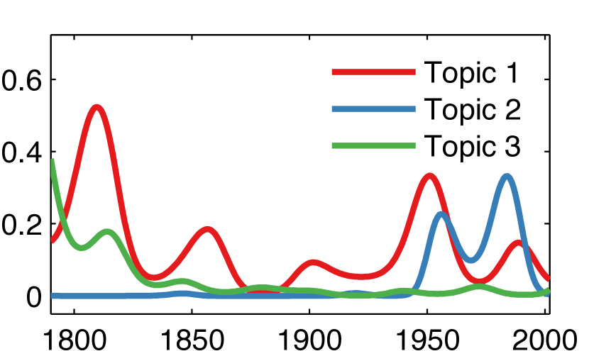
Figure 2: Activation functions over time for three topics.

Table 4: Learned topics.

Topic 1	Topic 2	Topic 3
military (0.074)	soviet (0.042)	tribes (0.142)
defense (0.061)	nations (0.035)	indian (0.124)
war (0.056)	security (0.022)	indians (0.116)
forces (0.051)	peace (0.021)	frontier (0.034)
force (0.041)	nuclear (0.020)	greater (0.027)

In Figure 2 we depict the activation functions (the mean of $r^{n,t}_{k}$) over time for three topics, and in Table 4 we show the top 5 words in each topic and the probability of the word under the topic. Topic 1 is a topic on war and we see it peak at most major conflicts that the United States was involved in. Topic 2 is about the Cold War and peaks at the beginning and end. Topic 3 regards Native Americans and is very prominent in addresses up to the 1850s and becomes less active in recent addresses. Figure 2 shows that the tGaP-PFA topic model is able to uncover multi-modal topic activations as well as localizing the topic usage in time.

7 Discussion

We have presented a framework for dependent random measures, that can be used as priors for a large class of nonparametric Bayesian models. Unlike previous work, our construction is applicable to any CRM and has the added benefit that the resultant dependent CRMs retain any existing conjugacy. We showed that many dependent random measures in the literature can actually be seen as specific cases of the thinned CRM framework. We demonstrated the effectiveness of the framework by using it to create a non-exchangeable latent feature model and a time-varying topic model. The models achieved superior predictive performance to exchangeable versions.

Appendix A Time-varying topic model

Recall that $w_{pnt}$ represents the number of occurrences of word $p$ in the $n$th document at time $t$, and that we decompose this as $w_{pnt}=\sum_{k=1}^{\infty}\tilde{w}_{pntk}$, where $\tilde{w}_{pntk}$ is the number of occurences attributed to topic $k$. In the generative process presented below, $p$ indexes the vocabulary, $t$ indexes the observed times of documents, $n$ indexes the documents at a time $t$ and takes values in $\{1,\ldots,N_{t}\}$, and $k$ indexes the topics. Additionally, $l$ indexes the kernel functions of the RVM (Tipping, 2001) with centers $m_{l}$, which we take to be the locations of the observations (although this is not necessary).

The generative process is as follows

$$\Gamma:=\sum_{k=1}^{\infty}\pi_{k}\delta_{(x_{k},\theta_{k})}\sim\mbox{CRM}(\nu_{G0}(d\pi)H(dx)G_{0}(d\theta))\;,$$ (5)

where $x_{k}:=(\omega_{0k},\dots,\omega_{Lk},\phi_{k})$; $\nu_{G0}(d\pi)=\pi^{-1}\exp(-\pi)d\pi$ is the Lévy measure of the gamma process with parameters $(1,1)$; $B_{0}(d\theta)$ is the $P$-dimensional Dirichlet distribution with parameter $\alpha_{\theta}$; and $H(dx)=H_{\phi}(d\phi)\prod_{l=0}^{L}H_{\omega}(d\omega_{l})$, where $H_{\phi}(d\phi)$ is the categorical distribution over the dictionary of kernel widths, and $H_{\omega}(d\omega_{l})\sim\text{NiG}(0,c_{0},d_{0})$ is drawn from the normal-inverse gamma distribution. The rest of the model is

$$p_{x_{k}}(t) =\Phi\big{(}\omega_{0k}+\textstyle{\sum_{l=1}^{L}}\omega_{lk}\exp(-\phi_{k}\left|\left|t-t_{l}\right|\right|_{2}^{2})\big{)}$$ (6)

$$\textstyle r_{k}^{n,t} \sim\text{Ber}(p_{x_{k}}(t))$$ (7)

$$\textstyle G_{n,t} :=\textstyle{\sum_{k=1}^{\infty}}r_{k}^{n,t}\pi_{k}\delta_{\theta_{k}}$$ (8)

$$\beta_{k}^{n,t} \sim\text{Ga}(e,1),n=1,\dots,N_{t},k\in\mathbb{N}$$ (9)

$$\tilde{w}_{pntk} \sim\text{Pois}(\theta_{kp}r_{k}^{n,t}\pi_{k}\beta_{k}^{n,t})$$ (10)

$$w_{pnt} =\sum_{k=1}^{\infty}\tilde{w}_{pntk}\sim\text{Pois}(\sum_{k=1}^{\infty}\theta_{kp}r_{k}^{n,t}\pi_{k}\beta_{k}^{n,t})$$ (11)

Appendix B Gibbs sampler

We use a truncated version of the model by fixing the number of atoms we will represent to $K$ and forming the (finite) random measure, $\Gamma_{K}:=\sum_{k=1}^{K}\pi_{k}\delta_{(x_{k},\phi_{k})}$, where $\pi_{k}\sim\text{Ga}(1/K,1)$, $x_{k}:=(\omega_{0k},\dots,\omega_{Lk},\phi_{k})$, $\omega_{lk}\sim\mbox{NiG}(0,c_{0},d_{0})$, and $\phi_{k}\sim\{\phi_{1}^{*},\dots,\phi_{d}^{*}\}$. In the limit, $K\rightarrow\infty$, $\Gamma_{K}\rightarrow\Gamma$ in distribution. This truncation allows for the derivation of a straight-forward Gibbs sampler. We assume $\mathcal{T}$ is the set of unique observed times.

We sample each of the variables in turn from their full conditional distributions. We use a standard data-augmentation technique for probit regression to sample the $\omega_{lk}$ variables by introducing an auxiliary variable $\tilde{r}^{n,t}_{k}\sim N(p_{x_{k}}(t),1)$ for each topic $k$ at each document $n$ at time $t$, such that

$$\begin{split}r_{k}^{n,t}=\begin{cases}1&\mbox{ if }\tilde{r}_{k}^{n,t}>0\\ 0&\mbox{ otherwise.}\end{cases}\end{split}$$

See Albert & Chib (1993) for details of the data augmentation. The conditional distributions are as follows.

• Topics, $\theta_{k}$.

  $$\theta_{k}|\ldots\sim\text{Dir}(\alpha_{\theta}+\tilde{w}_{1\cdot\cdot k},\ldots,\alpha_{\theta}+\tilde{w}_{P\cdot\cdot k})$$ (12)

  where $\tilde{w}_{p\cdot\cdot k}=\sum_{t\in\mathcal{T}}\sum_{n=1}^{N_{t}}\tilde{w}_{pntk}$.

• Global topic proportions, $\pi_{k}$.

  $$\pi_{k}|\ldots\sim\text{Ga}(\tilde{w}_{\cdot\cdot\cdot k}+1/K,\sum_{t\in\mathcal{T}}\sum_{n=1}^{N_{t}}\beta_{k}^{n,t}+1)$$ (13)

  where $\tilde{w}_{\cdot\cdot\cdot k}=\sum_{p=1}^{P}\sum_{t\in\mathcal{T}}\sum_{n=1}^{N_{t}}\tilde{w}_{pntk}$.

• Per-topic counts, $\tilde{w}_{pntk}$.

  $$(\tilde{w}_{pnt1},\dots,\tilde{w}_{pntK})|\ldots \sim\text{Mult}(w_{pnt};\xi_{pnt1},\ldots,\xi_{pntK}),$$

  $$\xi_{pntk} =\frac{\theta_{pk}r^{n,t}_{k}\pi_{k}\beta_{k}^{n,t}}{\sum_{j=1}^{K}\theta_{pj}r^{n,t}_{j}\pi_{j}\beta_{j}^{n,t}}$$ (14)

  and we ensure that the denominator is greater than $0$ by making sure that when sampling the $r^{n,t}_{k}$s, every document is not thinning at least one topic, i.e. $\forall t\forall n\exists j,r^{n,t}_{j}=1$.

• Per-document topic rate, $\beta_{k}^{n,t}$.

  $$\beta_{k}^{n,t}|\ldots\sim\text{Ga}(\tilde{w}_{\cdot ntk}+a,r^{n,t}_{k}\pi_{k}+1)$$ (15)

  where $\tilde{w}_{\cdot ntk}=\sum_{p=1}^{P}\tilde{w}_{pntk}$.

• Time-dependent indicators, $r^{n,t}_{k}$: There are three cases:

  1. $\forall j,r^{n,t}_{j}=0\rightarrow z^{n,t}_{k}=1$

  2. $\exists p,\tilde{w}_{pntk}>0\rightarrow r^{n,t}_{k}=1$

  3. $\forall p,\tilde{w}_{pntk}=0$

  Cases 1 and 2 are deterministic. For case 3 let $u_{pntk}\sim\text{Pois}(\rho_{p})$ with $\rho_{p}=\theta_{pk}\pi_{k}\beta_{k}^{n,t}$ denote the fictitious count of word $p$ in the $n$th document at time $t$ assigned to topic $k$ disregarding $r^{n,t}_{k}$. The $u_{pntk}$ allow us to determine whether $\tilde{w}_{pntk}=0$ because the topic has been thinned or because the topic is not popular (globally or for the individual document). Case 3 above then splits into the following cases:

  1. $\forall p,u_{pntk}=0,\;r^{n,t}_{k}=1$ with probability $\propto p(r^{n,t}_{k}=1)\prod_{p=1}^{P}\text{Pois}(0;\rho_{p})$

  2. $\exists p,u_{pntk}>0,\;r^{n,t}_{k}=0$ with probability $\propto p(r^{n,t}_{k}=0)\left(1-\prod_{p=1}^{P}\text{Pois}(0;\rho_{p})\right)$

  3. $\forall p,u_{pntk}=0,\;r^{n,t}_{k}=0$ with probability $\propto p(r^{n,t}_{k}=0)\prod_{p=1}^{P}\text{Pois}(0;\rho_{p})$

  We evaluate the three probabilities and sample from the resulting discrete distribution.

• RVM weights, $\omega_{lk}$. We introduce the auxiliary variables $\lambda_{lk}$ such that

  $$\begin{split}\lambda_{lk}&\sim\text{Ga}(c_{0},d_{0})\\ \omega_{lk}&\sim N(0,\lambda_{lk}^{-1})\,.\end{split}$$

  Let $\boldsymbol{\omega}_{k}=(\omega_{0k},\ldots,\omega_{Lk})^{T}$ be the vector of RVM weights and $\mathbf{\tilde{r}}_{k}$ be the vector of augmentation variables for all all time stamps, and

  $$K_{tk}=(1,K(t,m_{1},\phi_{k}),\ldots,K(t,m_{L},\phi_{k}))^{T}$$ (16)

  be the vector of the evaluation of the RVM kernels for time $t$. Then, the conditional of $\boldsymbol{\omega}_{k}$ is given by

  $$\boldsymbol{\omega}_{k}|\mathbf{\tilde{r}}_{k},\ldots\sim\text{N}(\xi,B)$$ (17)

  where $B=(\text{diag}(\lambda_{0k},\ldots,\lambda_{Lk})+K^{T}_{tk}\mathbf{\tilde{r}}_{k})^{-1}$ and $\xi=BK^{T}_{tk}\mathbf{\tilde{r}}_{k}$.

• RVM auxiliary variables, $\tilde{r}^{n,t}_{k}$.

  $$p(\tilde{r}^{n,t}_{k}|\ldots)\propto\begin{cases}\text{N}(K^{T}_{tk}\boldsymbol{\omega}_{k},1)\mathbf{1}(\tilde{r}^{n,t}_{k}>0),&r^{n,t}_{k}=1\\ \text{N}(K^{T}_{tk}\boldsymbol{\omega}_{k},1)\mathbf{1}(\tilde{r}^{n,t}_{k}<0),&r^{n,t}_{k}=0\end{cases}$$ (18)

  which is a truncated normal distribution that we sample using the inversion method described in Albert & Chib (1993).

• RVM precisions, $\lambda_{lk}$.

  $$\lambda_{lk}|\ldots\sim\text{Ga}\left(c_{0}+\frac{1}{2},d_{0}+\frac{1}{2}\omega^{2}_{lk}\right)$$ (19)

• RVM kernel widths, $\phi_{k}$. We assume a finite dictionary $\{\phi^{*}_{1},\ldots,\phi^{*}_{M}\}$ of possible values for the RVM kernel widths, and a uniform prior on these values,

  $$p(\phi_{k}=\phi^{*}_{m}|\ldots)\propto$$ (20)

  $$\frac{1}{M}\prod_{t\in\mathcal{T}}\prod_{n=1}^{N_{t}}\Phi(p_{\phi^{*}_{m}}(t))^{r^{n,t}_{k}}(1-\Phi(p_{\phi^{*}_{m}}(t)))^{1-r^{n,t}_{k}}$$

  where we have denoted the thinning function as a function of $\phi^{*}$ as the other variables are held fixed.

Appendix C Perplexity computation

Similarly to Zhou et al. (2012b), given $B$ samples of the model parameters and latent variables we compute a Monte Carlo estimate of the held-out perplexity for unobserved counts $Y=[y_{p}^{n,t}]$ as

$$\exp\Bigg{(} \frac{1}{y_{\cdot}^{\cdot,\cdot}}\sum_{p=1}^{P}\sum_{t\in\mathcal{T}}\sum_{n=1}^{N_{t}}y_{p}^{n,t}\times$$ (21)

$$\log\frac{\sum_{b=1}^{B}\sum_{k=1}^{K}\theta^{(b)}_{pk}\pi^{(b)}_{k}r_{ntk}{{}^{(b)}}\beta^{(b)}_{ntk}}{\sum_{b=1}^{B}\sum_{p=1}^{P}\sum_{k=1}^{K}\theta^{(b)}_{pk}\pi^{(b)}_{k}r_{ntk}{{}^{(b)}}\beta^{(b)}_{ntk}}\Bigg{)}$$

where we have used a superscript $b$ to denote the $b$th sample of the parameters and latent variables and $y_{\cdot}^{\cdot,\cdot}=\sum_{p=1}^{P}\sum_{t\in\mathcal{T}}\sum_{n=1}^{N_{t}}y_{p}^{n,t}$ denotes the held-out number of occurrences of word $p$ in the $n$th document at time $t$.

References

- Albert & Chib (1993) Albert, J.H. and Chib, S. Bayesian analysis of binary and polychotomous response data. JASA, 88(422):669–679, 1993.
- Blei & Lafferty (2006) Blei, D. M. and Lafferty, J. D. Dynamic topic models. In ICML, 2006.
- Blei & Lafferty (2007) Blei, D. M. and Lafferty, J. D. A correlated topic model of science. AAS, 1(1):17–35, 2007.
- Blei et al. (2003) Blei, D. M., Ng, A. Y., and Jordan, M. I. Latent dirichlet allocation. J. Mach. Learn. Res., 3:993–1022, March 2003.
- Caron et al. (2007) Caron, F., Davy, M., and Doucet, A. Generalized Polya urn for time-varying Dirichlet process mixtures. In UAI, 2007.
- Chung & Dunson (2011) Chung, Y. and Dunson, D.B. The local Dirichlet process. Ann. Inst. Statist. Math., 63(1):59–80, 2011.
- Duan et al. (2007) Duan, J.A., Guindani, M., and Gelfand, A.E. Generalized spatial Dirichlet process models. Biometrika, 94(4):809–825, 2007.
- Goodman et al. (2008) Goodman, N. D., Mansinghka, V. K., Roy, D. M., Bonawitz, K., and Tenenbaum, J. B. Church: A language for generative models. In UAI, 2008.
- Griffin (2007) Griffin, J.E. The Ornstein-Uhlenbeck Dirichlet process and other time-varying processes for Bayesian nonparametric inference. Technical report, Department of Statistics, University of Warwick, 2007.
- Griffin & Steel (2006) Griffin, J.E. and Steel, M.F.J. Order-based dependent Dirichlet processes. JASA, 101(473):179–194, 2006.
- Griffiths & Ghahramani (2005) Griffiths, T. L. and Ghahramani, Z. Infinite latent feature models and the Indian buffet process. In NIPS, 2005.
- Ibrahim et al. (2005) Ibrahim, J.G., Chen, M.H., and Sinha, D. Bayesian survival analysis. Wiley, 2005.
- Kingman (1967) Kingman, J. F. C. Completely random measures. Pacific Journal of Mathematics, 21(1):59–78, 1967.
- Kingman (1993) Kingman, J.F.C. Poisson processes. OUP, 1993.
- Lin et al. (2010) Lin, D., Grimson, E., and Fisher, J. Construction of dependent Dirichlet processes based on Poisson processes. In NIPS, 2010.
- MacEachern (1999) MacEachern, S.N. Dependent nonparametric processes. In Proc. Sect. Bayesian Statist. Sci., pp. 50–55, 1999.
- Manning et al. (2008) Manning, C. D., Raghavan, P., and Schütze, H. Introduction to Information Retrieval. Cambridge University Press, New York, NY, USA, 2008.
- Miller (2011) Miller, K. Bayesian Nonparametric Latent Feature Models. PhD thesis, EECS Department, U.C. Berkeley, 2011.
- Paisley & Carin (2009) Paisley, J. and Carin, L. Nonparametric factor analysis with beta process priors. In ICML, 2009.
- Paisley et al. (2011) Paisley, J. W., Wang, C., and Blei, D. M. The discrete infinite logistic normal distribution for mixed-membership modeling. In AISTATS, 2011.
- Rao & Teh (2009) Rao, V. and Teh, Y.W. Spatial normalized gamma processes. In NIPS, 2009.
- Ren et al. (2011) Ren, L., Wang, Y., Dunson, D., and Carin, L. The kernel beta process. In NIPS, 2011.
- Saeedi & Bouchard-Côté (2011) Saeedi, A. and Bouchard-Côté, A. Priors over recurrent continuous time processes. In NIPS, 2011.
- Sudderth & Jordan (2009) Sudderth, E. and Jordan, M.I. Shared segmentation of natural scenes using dependent Pitman-Yor processes. In NIPS, 2009.
- Thibaux & Jordan (2007) Thibaux, R. and Jordan, M.I. Hierarchical beta processes and the Indian buffet process. In AISTATS, 2007.
- Tipping (2001) Tipping, M. E. Sparse Bayesian learning and the relevance vector machine. JMLR, 1:211–244, 2001.
- Titsias (2007) Titsias, M. The infinite gamma-Poisson feature model. In NIPS, 2007.
- Wang et al. (2008) Wang, C., Blei, D. M., and Heckerman, D. Continuous time dynamic topic models. In UAI, 2008.
- Wang & McCallum (2006) Wang, X. and McCallum, A. Topics over time: a non-markov continuous-time model of topical trends. In KDD, 2006.
- Williamson et al. (2010) Williamson, S., Orbanz, P., and Ghahramani, Z. Dependent Indian buffet processes. In AISTATS, 2010.
- Wood et al. (2006) Wood, F., Griffiths, T. L., and Ghahramani, Z. A non-parametric Bayesian method for inferring hidden causes. In UAI, pp. 536–543, 2006.
- Zhou et al. (2011) Zhou, M., Yang, H., Sapiro, G., Dunson, D., and Carin, L. Dependent hierarchical beta process for image interpolation and denoising. In AISTATS, 2011.
- Zhou et al. (2012a) Zhou, M., Chen, H., Paisley, J. W., Ren, L., Li, L., Xing, Z., Dunson, D. B., Sapiro, G., and Carin, L. Nonparametric Bayesian dictionary learning for analysis of noisy and incomplete images. IEEE Trans. Image Process., 21(1):130–144, 2012a.
- Zhou et al. (2012b) Zhou, M., Hannah, L. A., Dunson, D. B., and Carin, L. Beta-negative binomial process and Poisson factor analysis. In AISTATS, 2012b.