QUANTUM GRAPH WALKS II
Quantum walks on graph coverings

Abstract

We give a new determinant expression for the characteristic polynomial of the bond scattering matrix of a quantum graph $G$. Also, we give a decomposition formula for the characteristic polynomial of the bond scattering matrix of a regular covering of $G$. Furthermore, we define an $L$-function of $G$, and give a determinant expression of it. As a corollary, we express the characteristic polynomial of the bond scattering matrix of a regular covering of $G$ by means of its $L$-functions. As an application, we introduce three types of quantum graph walks, and treat their relation.

2000 Mathematical Subject Classification: 81Q10, 05C50, 05C60, 81P68.
Key words and phrases : quantum graph, scattering matrix, quantum walk, graph covering, $L$-function

The contact author for correspondence:

1 Introduction

A quantum graph identifies edges of an ordinary graph with closed intervals generating a metric graph, and has an operator acting on functions defined on the collection of intervals. The review and book on quantum graphs are Exner and Šeba [8], Kuchment [25], Gnutzmann and Smilansky [11], for examples.

One of interest on quantum graphs is the spectral question of quantum graphs. This is approached through a trace formula. The first graph trace formula was derived by Roth [29]. Kottos and Smilansy [24] introduced a contour integral approach to the trace formula starting with a secular equation based on the scattering matrix of plane-waves on the graph. Solutions of the secular equation corresponds to the points in the spectrum of the quantum graph.

Trace formulas express spectral functions like the density of states or heat kernel as sums over periodic orbits on the graph. This fact is related to the Ihara zeta function. furthermore, the spectral determinant of the Laplacian on a quantum graph is closely related to the Ihara zeta function of a graph (see [5,6,13,14]). Smilansky [32] considered spectral zeta functions and trace formulas for (discrete) Laplacians on ordinary graphs, and expressed some determinant on the bond scattering matrix of a graph $G$ by using the characteristic polynomial of its Laplacian.

As a quantum counterpart of the classical random walk, the quantum walk has recently attracted much attention for various fields. The review and book on quantum walks are Ambainis [1], Kempe [19], Kendon [20], Konno [21], Venegas-Andraca [39], for examples.

In 1988, Gudder defined discrete-time quantum walk on a graph from the view point of quantum measure introduced as a quantum analogue of probability measure in his book [12]. The Grover walk on a graph was formulated in [41]. We can see that there are many applications of the Grover walk to quantum spatial search algorithms in the review by Ambainis [1], for example. As a generalization of the Grover walk, Szegedy [37] introduced the Szegedy walk on a graph related to a transition matrix of a random walk on the same graph.

Recently, the relation between quantum graphs and quantum walks on graphs are pointed out (see [31,38]). Higuchi, Konno, Sato and Segawa [16] introduced a quantum walks related quantum graphs. As a sequential work of this manuscript and [16], we show the relationship between a quantum walk and a scattering amplitude via discrete Laplacian in [17].

Zeta functions of graphs were originally defined for regular graphs by Ihara [18]. This is the Ihara zeta function of a graph. In [18], he showed that their reciprocals are explicit polynomials. A zeta function of a regular graph $G$ associated with a unitary representation of the fundamental group of $G$ was developed by Sunada [35,36]. Hashimoto [15] treated multivariable zeta functions of bipartite graphs. Bass [4] generalized Ihara’s result on the zeta function of a regular graph to an irregular graph and showed that its reciprocal is again a polynomial. A decomposition formula for the Ihara zeta function of a regular covering of a graph was obtained by Stark and Terras [34], and independently, Mizuno and Sato [27].

The discrete-time quantum walk on a graph is closely related to the Ihara zeta function of a graph. Ren et al. [28] found an interesting relation between the Ihara zeta function and the discrete-time quantum walk on a graph, and showed that the positive support of the transition matrix of the discrete-time quantum walk is equal to the Perron-Frobenius operator (the edge matrix) related to the Ihara zeta function. Konno and Sato [22] gave the characteristic polynomials of the support of the transition matrix of the discrete-time quantum walk and its positive support, and so obtained the other proofs of the results on spectra for them by Emms et al. [7].

In this paper, we present a new determinant expression for the scattering matrix of a quantum graph. In Section 2, we state a short review on quantum graphs. We consider the Schrödinger equation and the boundary conditions of a quantum graph from a view point of arcs (oriented edges) of the graph under Ref. [16], and present two types of the scattering matrix of a quantum graph. In Section 3, we treat a quantum walk on a graph, and discuss the relation between four quantum graph walks induced by a quantum graph. We clarify that these walks are in spatial and temporal reversal relation. In Section 4, we present a new determinant expression for the characteristic polynomial of the scattering matrix of a quantum graph by using the method of Watanabe and Fukumizu [40]. In Section 5, we give a formulation for the Schrödinger equation and the boundary conditions of a regular covering of a quantum graph, and propose a type of the scattering matrix of a quantum graph whose base graph is a regular covering of a graph. Furthermore, we give a decomposition formula for the characteristic polynomial of the scattering matrix of a regular covering. In Section 6, we define an $L$-function of a graph and give a determinant expression for it. As a corollary, we express the determinant for the characteristic polynomial of the scattering matrix of a regular covering as a product of $L$-functions. In Section 7, we express the above $L$-function of a graph by using the Euler product.

2 Scattering matrix of a quantum graph

We present a review on a quantum graph.

Graphs treated here are finite. Let $G$ be a connected graph (possibly with multiple edges and loops) with the set $V(G)$ of vertices and the set $E(G)$ of unoriented edges. We write $uv$ for an edge joining two vertices $u$ and $v$. For $uv\in E(G)$, an arc $(u,v)$ is the oriented edge from $u$ to $v$. Set $D(G)=\{(u,v),(v,u)\mid uv\in E(G)\}$. For $e=(u,v)\in D(G)$, set $u=o(e)$ and $v=t(e)$. Furthermore, let $e^{-1}=(v,u)$ be the inverse arc of $e=(u,v)$.

Let $G$ be a connected graph with $V(G)=\{1,\ldots,n\}$ and $D(G)=\{e_{1},\ldots,e_{m},e^{-1}_{1},\ldots,e^{-1}_{m}\}$. Arrange vertices of $G$ as follows: $1<2<\cdots<n$. Furthermore, let $d_{j}=\deg j,j\in V(G)$. For each edge $ij\in E(G)$, let $L_{ij}$ and $A_{ij}$ be the length and the vector potential of $ij$, respectively. If $ij\in E(G)$, then assign a variable $x$ in the interval $[0,L_{ij}]$ such that $x=0$ and $x=L_{ij}$ corresponds to $i$ and $j$, respectively, and an intermediate point $z$ of $ij$ corresponds to the distance between $i$ and $z$.

For $e=(i,j)\in D(G)$, set

$$L_{e}=L_{ij},A_{e}=\left\{\begin{array}[]{ll}A_{ij}&\mbox{if $i<j$, }\\ -A_{ij}&\mbox{if $i>j$. }\end{array}\right.$$

Note that

$$L_{e}=L_{e^{-1}},\ \ A_{e^{-1}}=-A_{e}.$$

Let $e=(j,l)\in D(G)$. Then the Schrödinger equation for $e$ is given by

$$\left(-{\bf i}{\rm\frac{d}{dx}}+A_{e}\right)^{2}\Psi{}_{e}(x)=k^{2}\Psi{}_{e}(x)$$ (1)

under the following three conditions:

1. $\Psi{}_{e}(x)=\Psi{}_{e^{-1}}(L_{jl}-x)$;

2. The continuity: $\Psi{}_{e}(0)=\phi{}_{j}$ and $\Psi{}_{e}(L_{jl})=\phi{}_{l}$;

3. The cuurent conservation:

   $$\sum_{o(e)=j}\left(-{\bf i}{\rm\frac{d}{dx}}+A_{e}\right)\Psi{}_{e}(x)\bigg{|}_{x=0}=-{\bf i}\lambda{}_{j}\phi{}_{j},\forall j\in V(G),$$

   where $(\phi{}_{1},\ldots,\phi{}_{n})\in{\bf C}^{n}$.

The solution of (1) is given by

$$\Psi{}_{e}(x)=(a_{e}e^{-{\bf i}kx}+b_{e}e^{{\bf i}kx})e^{-{\bf i}A_{e}x},{\bf i}=\sqrt{-1}.$$ (2)

By condition 1, we have

$$a_{e}=b_{e^{-1}}e^{{\bf i}L_{e}(k+A_{e})}\ and\ b_{e}=a_{e^{-1}}e^{-{\bf i}L_{e}(k-A_{e})}.$$ (3)

By condition 2, we have

$$a_{e_{1}}+b_{e_{1}}=a_{e_{2}}+b_{e_{2}}=\cdots=a_{e_{d_{j}}}+b_{e_{d_{j}}}=\phi{}_{j},$$ (4)

where $e_{1},e_{2},\ldots,e_{d_{j}}$ are arcs emanating from $j$, and $d_{j}=\deg j$. By condition 3, we have

$$\sum^{d_{j}}_{r=1}(a_{e_{r}}-b_{e_{r}})={\bf i}\lambda{}_{j}\phi{}_{j}=\frac{{\bf i}\lambda{}_{j}}{d_{j}}\sum^{d_{j}}_{r=1}(a_{e_{r}}+b_{e_{r}}).$$ (5)

Thus,

$$\sum^{d_{j}}_{r=1}b_{e_{r}}=\frac{1-{\bf i}\lambda{}_{j}/kd_{j}}{1+{\bf i}\lambda{}_{j}/kd_{j}}\sum^{d_{j}}_{r=1}a_{e_{r}}.$$ (6)

By (4), for $1\leq p\leq d_{j}$, we have

$$b_{e_{p}}=\phi{}_{j}-a_{e_{p}}=\frac{1}{d_{j}}\sum^{d_{j}}_{r=1}(a_{e_{r}}+b_{e_{r}})-a_{e_{p}}.$$

By (6),

$$b_{e_{p}}=\sum^{d_{j}}_{r=1}\left(\frac{2{\bf i}k}{{\bf i}kd_{j}-\lambda{}_{j}}-\delta{}_{e_{r}e_{p}}\right)a_{e_{r}},$$ (7)

where $\delta{}_{e_{r}e_{p}}$ is the Kronecker delta. By (3) and (7), we have

$$a_{e_{p}}=b_{e^{-1}_{p}}e^{{\bf i}L_{e_{P}}(k+A_{e_{p}})}=\sum^{d_{l}}_{r=1}(\frac{2{\bf i}k}{{\bf i}kd_{l}-\lambda{}_{l}}-\delta{}_{f_{r}e^{-1}_{p}})e^{{\bf i}L_{e_{p}}(k+A_{e_{p}})}a_{f_{r}},$$ (8)

where $f_{1},\ldots,f_{d_{l}}$ are arcs emanating from $l$.

Now, we introduce the Gnutzmann-Smilansky type of the bond scattering matrix of a quantum graph. Let

$$c_{e^{-1}}=a_{e}\ for\ each\ e\in D(G).$$

Then we have

$$c_{e^{-1}_{p}}=\sum^{d_{l}}_{r=1}\left(\frac{2{\bf i}k}{{\bf i}kd_{l}-\lambda{}_{l}}-\delta{}_{f^{-1}_{r}e_{p}}\right)e^{{\bf i}L_{e^{-1}_{p}}(k-A_{e^{-1}_{p}})}c_{f^{-1}_{r}}.$$

Thus, for each arc $e$ with $o(e)=l$,

$$c_{e}=\sum_{t(f)=l}\sigma{}^{(l)}_{ef}(k)e^{{\bf i}L_{e}(k-A_{e})}c_{f},$$ (9)

where

$$\sigma{}^{(l)}_{ef}(k)=\frac{2{\bf i}k}{{\bf i}kd_{l}-\lambda{}_{l}}-\delta{}_{e^{-1}f}.$$

The vertex scattering matrix ${\bf S}(k)=(S_{ef}(k))_{e,f\in D(G)}$ of $G$ is defined by

$$S_{ef}(k)=\left\{\begin{array}[]{ll}\sigma^{(t(f))}_{ef}(k)&\mbox{if $t(f)=o(e)$, }\\ 0&\mbox{otherwise. }\end{array}\right.$$

Next, the bond propagation matrix ${\bf T}(k)=(T_{ef}(k))_{e,f\in D(G)}$ of $G$ is defined by

$$T_{ef}(k)=\left\{\begin{array}[]{ll}\exp{({\bf i}L_{e}(k-A_{e}))}&\mbox{if $e=f$, }\\ 0&\mbox{otherwise. }\end{array}\right.$$

Then we define the Gnutzmann-Smilansky type of the bond scattering matrix ${\bf U}_{GS}(k)={\bf U}_{GS}(G,k)$ by

$${\bf U}_{GS}(k)={\bf T}(k){\bf S}(k).$$ (10)

By (9), we have

$${\bf U}_{GS}(k){\bf c}={\bf c},$$ (11)

where ${\bf c}={}^{t}(c_{1},c_{2},\ldots,c_{2m})$. Then (9) holds if and only if

$$\det({\bf I}_{2m}-{\bf U}_{GS}(k))=0.$$

Now, we introduce another type of the bond scattering matrix of a quantum graph. By (6),

$$\sum^{d_{j}}_{r=1}a_{e_{r}}=\frac{1+{\bf i}\lambda{}_{j}/kd_{j}}{1-{\bf i}\lambda{}_{j}/kd_{j}}\sum^{d_{j}}_{r=1}b_{e_{r}}.$$ (12)

By (4), for $1\leq p\leq d_{j}$, we have

$$a_{e_{p}}=\phi{}_{j}-b_{e_{p}}=\frac{1}{d_{j}}\sum^{d_{j}}_{r=1}(a_{e_{r}}+b_{e_{r}})-b_{e_{p}}.$$

By (12),

$$a_{e_{p}}=\sum^{d_{j}}_{r=1}\left(\frac{2{\bf i}k}{{\bf i}kd_{j}+\lambda{}_{j}}-\delta{}_{e_{r}e_{p}}\right)b_{e_{r}}.$$ (13)

By (3), we have

$$a_{e_{p}}=\sum^{d_{j}}_{r=1}\left(\frac{2{\bf i}k}{{\bf i}kd_{j}+\lambda{}_{j}}-\delta{}_{e_{r}e_{p}}\right)e^{-{\bf i}L_{e_{r}}(k-A_{e_{r}})}a_{e^{-1}_{r}}.$$ (14)

By (8) and (14), we have the following result.

Proposition 1.

In a quantum graph $G$, for an arc $e=(j,l)\in D(G)$,

$$\sum_{o(f)=j}\left(\frac{2{\bf i}k}{{\bf i}kd_{j}+\lambda{}_{j}}-\delta{}_{fe}\right)e^{-{\bf i}L_{f}(k-A_{f})}a_{f^{-1}}=\sum_{o(g)=l}\left(\frac{2{\bf i}k}{{\bf i}kd_{l}-\lambda{}_{l}}-\delta{}_{ge^{-1}}\right)e^{{\bf i}L_{e}(k+A_{e})}a_{g}.$$

On the other hand, for an arc $e$ such that $o(e)=j$, (13) is changed into

$$\begin{array}[]{rcl}a_{e}&=&\sum_{t(f)=j}\left(\frac{2{\bf i}k}{{\bf i}kd_{j}+\lambda{}_{j}}-\delta{}_{fe^{-1}}\right)e^{-{\bf i}L_{f}(k+A_{f})}a_{f}\\ &&\\ &=&\sum_{t(f)=j}\sigma{}^{(j)}_{ef}(-k)e^{-{\bf i}L_{f}(k+A_{f})}a_{f},\end{array}$$ (15)

where

$$\sigma{}^{(j)}_{ef}(-k)=\frac{2{\bf i}k}{{\bf i}kd_{j}+\lambda{}_{j}}-\delta{}_{e^{-1}f}.$$

The $(e,f)$-array of the vertex scattering matrix ${\bf S}(-k)=(S_{ef}(-k))_{e,f\in D(G)}$ of $G$ is given by

$$S_{ef}(-k)=\left\{\begin{array}[]{ll}\sigma^{(t(f))}_{ef}(-k)&\mbox{if $t(f)=o(e)$, }\\ 0&\mbox{otherwise. }\end{array}\right.$$

Furthermore, the $(e,f)$-array of the bond propagation matrix ${\bf T}(-k)=(T_{ef}(-k))_{e,f\in D(G)}$ of $G$ is given by

$$T_{ef}(-k)=\left\{\begin{array}[]{ll}\exp{(-{\bf i}L_{e}(k+A_{e}))}&\mbox{if $e=f$, }\\ 0&\mbox{otherwise. }\end{array}\right.$$

Then we define another type of the bond scattering matrix ${\bf U}_{HKSS}(k)={\bf U}_{HKSS}(G,k)$ by

$${\bf U}_{HKSS}(k)={\bf S}(-k){\bf T}(-k).$$ (16)

By (15), we have

$${\bf U}_{HKSS}(k){\bf a}={\bf a},$$ (17)

where ${\bf a}={}^{t}(a_{1},a_{2},\ldots,a_{2m})$. Then (14) holds if and only if

$$\det({\bf I}_{2m}-{\bf U}_{HKSS}(k))=0.$$

Now, we state the relation between the Gnutzmann-Smilansky scattering matrix and another scattering matrix of a quantum graph.

At first, let $j\in V(G)$, and $e_{1},e_{2},\ldots,e_{d_{j}}$ be arcs emanating from $j$. Furthermore, let

$${\bf a}_{j}={}^{t}(a_{e_{1}},\ldots,a_{e_{d_{j}}}),{\bf b}_{j}={}^{t}(b_{e_{1}},\ldots,b_{e_{d_{j}}}),x_{j}=x_{j}(k)=\frac{2{\bf i}k}{{\bf i}kd_{j}-\lambda{}_{j}}.$$

Then (7) implies that

$${\bf b}_{j}=(x_{j}{\bf J}_{d_{j}}-{\bf I}_{d_{j}}){\bf a}_{j},\ \ \ \ \ \ (*)$$

where ${\bf J}_{d_{j}}$ is the $d_{j}\times d_{j}$ matrix with all one. Thus, putting

$${\bf F}_{j}=x_{j}{\bf J}_{d_{j}}-{\bf I}_{d_{j}}.$$

the above equation is reexpressed by

$${\bf b}_{j}={\bf F}_{j}{\bf a}_{j}.$$

Here

$$\det{\bf F}_{j}=(d_{j}x_{j}-1)(-1)^{d_{j}-1}\neq 0$$

and

$${\bf F}^{-1}_{j}=x_{j}(-k){\bf J}_{d_{j}}-{\bf I}_{d_{j}}.$$

Let

$${\bf a}={}^{t}({\bf a}_{1},\ldots,{\bf a}_{n}),{\bf b}={}^{t}({\bf b}_{1},\ldots,{\bf b}_{n}),{\bf F}={\bf F}_{1}\oplus\ldots\oplus{\bf F}_{n}.$$

Then we have

$${\bf b}={\bf F}{\bf a}\ and\ {\bf a}={\bf F}^{-1}{\bf b}.$$ (18)

Next, let the $2m\times 2m$ diagonal matrix ${\bf R}(k)=(R_{ef}(k))$ be given by

$$R_{ef}(k)=\left\{\begin{array}[]{ll}e^{{\bf i}L_{e}(k+A_{e})}&\mbox{if $e=f$, }\\ 0&\mbox{otherwise. }\end{array}\right.$$

Since $a_{e}=b_{e^{-1}}e^{{\bf i}L_{e}(k+A_{e})}$, we have

$${\bf a}={\bf R}(k){\bf J}_{0}{\bf b},$$ (19)

where ${\bf J}_{0}=(J_{ef})$ is given by

$$J_{ef}=\left\{\begin{array}[]{ll}1&\mbox{if $f=e^{-1}$, }\\ 0&\mbox{otherwise. }\end{array}\right.$$

Note that ${\bf J}^{-1}_{0}={\bf J}_{0}$. By (18) and (19), (8) is rewritten as follows:

$${\bf a}={\bf R}(k){\bf J}_{0}{\bf F}{\bf a}.$$ (20)

Furthermore, by (19),

$${\bf b}={\bf J}_{0}{\bf R}(k)^{-1}{\bf a},$$

and so, (14) is also rewritten as follows:

$${\bf a}={\bf F}^{-1}{\bf b}={\bf F}^{-1}{\bf J}_{0}{\bf R}(k)^{-1}{\bf a}.$$ (21)

By (20) and (21), we obtain the following equivalent expression to Proposition 1:

$${\bf a}={\bf R}(k){\bf J}_{0}{\bf F}{\bf a}={\bf F}^{-1}{\bf J}_{0}{\bf R}(k)^{-1}{\bf a}.$$

By the way, it holds that

$${\bf T}(k)={\bf J}_{0}{\bf R}(k){\bf J}_{0}\ and\ {\bf S}(k)={\bf F}{\bf J}_{0}.$$

Thus,

$${\bf U}_{GS}(k)={\bf T}(k){\bf S}(k)={\bf J}_{0}{\bf R}(k){\bf J}_{0}{\bf F}{\bf J}_{0}.$$ (22)

Furthermore, we have

$${\bf T}(-k)={\bf R}(k)^{-1}\ and\ {\bf S}(-k)={\bf F}^{-1}{\bf J}_{0}.$$

Thus,

$${\bf U}_{HKSS}(k)={\bf S}(-k){\bf T}(-k)={\bf F}^{-1}{\bf J}_{0}{\bf R}(k)^{-1}.$$ (23)

By (22), (23), we obtain the following result.

Proposition 2.

In a quantum graph $G$,

$${\bf U}_{GS}(k)={\bf J}_{0}{\bf U}^{-1}_{HKSS}(k){\bf J}_{0}.$$

3 Quantum graph walks

At first, we state a short review on a discrete-time quantum walk on a graph.

Let $G$ be a graph with $n$ vertices and $m$ edges. For $v\in V(G)$, let $N^{+}(v)=\{e\in D(G)\mid o(e)=v\}$. The we consider a quantum walk over $D(G)$. For each arc $e=(u,v)\in D(G)$, the pure state is given by $\vec{x}_{e}=\vec{x}_{uv}=|e\rangle=|u,v\rangle\in{\mathbb{C}}^{2m}$ such that $\{|e\rangle\mid e\in D(G)\}$ is the normal orthogonal system of the $2m$-dimensional Hilbert space ${\mathbb{C}}^{2m}$. ${\cal H}=\ell{}^{2}(D(G))={\rm span}\{|e\rangle\mid e\in D(G)\}$ is called the total space of a quantum walk on $G$. Then we have

$${\cal H}=\bigoplus_{v\in V(G)}{\cal H}_{v}\ and\ {\cal H}_{v}\cong{\rm span}\{|e\rangle\mid e\in N^{+}(v)\}.$$

Let $(u,v),(w,x)\in D(G)$. Then the transition from $(u,v)$ to $(w,x)$ occurs if $v=w$. The state $\psi$ of a quantum walk on $G$ is defined by

$$\psi=\sum_{e\in D(G)}\alpha{}_{e}|e\rangle,\ \alpha{}_{e}\in{\mathbb{C}},$$

where $\sum_{e\in D(G)}|\alpha{}_{e}|^{2}=1$. Furthermore, the probability which the walk is at the arc $e$ is given by $|\alpha{}_{e}|^{2}$.

The time evolution of a quantum walk on $G$ is given by a unitary matrix ${\bf U}$. By the definition of the transition, ${\bf U}=(U_{ef})_{e,f\in D(G)}$ is given as follows so that ${\bf U}$ is unitary:

$$U_{ef}=\left\{\begin{array}[]{ll}{\rm nonzero\ complex\ number}&\mbox{if $t(e)=o(f)$ (or $t(f)=o(e)$), }\\ 0&\mbox{otherwise. }\end{array}\right.$$

For an initial state $\psi{}_{0}$ with $||\psi{}_{0}||=1$, the time evolution is the iteration $\psi{}_{0}\mapsto\psi{}_{1}\mapsto\ldots$ of ${\bf U}$ such that

$$\psi{}_{j}={\bf U}^{j}\psi{}_{0},\ j\in{\bf N}.$$

Now, we explain a quantum walk called coined quantum walks on a graph $G$. Set $V(G)=\{1,\ldots,n\}$. Then we choose a sequence of unitary operators $\{{\bf H}_{j}\}{}_{j\in V(G)}$, where ${\bf H}_{j}$ is a $d_{j}$-dimensional operator on ${\cal H}_{j}$. Then we present two types of time evolutions ${\bf U}^{(G)}$ and ${\bf U}^{(A)}$ of quantum walks, respectively:

$${\bf U}^{(G)}={\bf H}{\bf J}_{0};{\bf U}^{(A)}={\bf J}_{0}{\bf H},$$

where ${\bf H}=\bigoplus_{j\in V(G)}{\bf H}_{j}$. ${\bf U}^{(G)}$ and ${\bf U}^{(A)}$ are called Gudder type and Ambainis type, respectively. The elements of ${\bf U}^{(G)}$(or ${\bf U}^{(A)}$) is nonzero if $t(f)=o(e)$ (or $t(e)=o(f)$). The first type determined by ${\bf U}^{(G)}$ is a generalization of Gudder [12] (1988) of $d$-dimensional lattice case. The second one ${\bf U}^{(A)}$ is motivated by the most popular time evolution for the study of QWs by Ambainis et al [2] (2001).

Next, we treat a quantum graph walk. Let $G$ be a connected graph $n$ vertices $1,\ldots,n$, and $m$ edges, and let $L:D(G)\longrightarrow{\mathbb{R}}^{+}$ and $A:D(G)\longrightarrow{\mathbb{R}}$ be the length and the magnetic flux of arcs of $G$, respectively. Let $\lambda:V(G)\longrightarrow{\mathbb{C}}$ be the parameters in the boundary condition III. The quantum graph walk with parameters $(L,A,\lambda)$ is defined as a quantum walk on $G$ by the Ambainis type time evolution $\tilde{{\bf U}}$ with the flip flop ${\bf J}_{0}$ and the following local quantum coin ${\bf H}_{j}=((H_{j})_{ef})_{e,f\in N^{+}(j)}$ at a vertex $j\in V(G)$:

$$(H_{j})_{ef}=\left(\frac{2{\bf i}k}{d_{j}{\bf i}k-\lambda{}_{j}}-\delta{}_{ef}\right)e^{{\bf i}L_{e}(k-A_{e})},\ e,f\in N^{+}(j).$$

Note that

$$\tilde{{\bf U}}={\bf J}_{0}{\bf H},\ {\bf H}={\bf H}_{1}\oplus\cdots\oplus{\bf H}_{n}.$$ (24)

For brevity, this quantum graph walk is denoted by $\tilde{{\bf U}}$. By the way, the quantum coin is reexpressed by

$${\bf H}={\bf T}(k){\bf F}.$$

Furthermore, recall that

$${\bf T}(k)={\bf J}_{0}{\bf R}(k){\bf J}_{0},$$

Using these relation implies

$${\bf H}={\bf J}_{0}{\bf R}(k){\bf J}_{0}{\bf F}.$$ (25)

By (24) and (25), we have

$$\tilde{{\bf U}}={\bf J}_{0}{\bf T}(k){\bf F}={\bf R}(k){\bf J}_{0}{\bf F}.$$ (26)

By (20), (8) is rewritten as follows:

$${\bf a}=\tilde{{\bf U}}{\bf a}.$$ (27)

Next, we can interpret two scattering matrices ${\bf U}_{GS}(k)$, and ${\bf U}_{HKSS}(k)$ which have discussed in the previous section as two kinds of quantum graph walks in the following sence. By (22) and (26), we have

$${\bf U}_{GS}(k)={\bf J}_{0}{\bf R}(k){\bf J}_{0}{\bf F}{\bf J}_{0}={\bf J}_{0}\tilde{{\bf U}}{\bf J}_{0}.$$ (28)

By (23) and (26), we have

$${\bf U}_{HKSS}(k)={\bf F}^{-1}{\bf J}_{0}{\bf R}(k)^{-1}=\tilde{{\bf U}}^{-1}.$$ (29)

By the forms of ${\bf U}_{GS}(k)$ and ${\bf U}_{HKSS}(k)$, ${\bf U}_{GS}(k)$ and ${\bf U}_{HKSS}(k)$ are Gudder type quantum graph walks. Furthermore, we introduce the third quantum graph walk of $G$ with the following time evolution:

$${\bf U}^{\prime}={\bf J}_{0}{\bf H}^{-1}.$$ (30)

This is an Ambainis type quantum graph walk.

As a consequence, the following result in relation to the quantum graph and corresponding four kinds of quantum graph walks holds.

Theorem 1.

In the quantum graph $G$ with parameters $(L,A,\lambda)$, the following statements are equivalent:

1. The Schrödinger equation (1) with the boundary conditions I. II. III has a nontrivial solution $\{\Psi{}_{e}\}{}_{e\in D(G)}$;

2. The time evolution $\tilde{{\bf U}}$ of the quantum graph walk has the eigenvalue 1.

3. The time evolution ${\bf U}_{GS}(k)$ of the quantum graph walk has the eigenvalue 1.

4. The time evolution ${\bf U}_{HKSS}(k)$ of the quantum graph walk has the eigenvalue 1.

5. The time evolution ${\bf U}^{\prime}$ of the quantum graph walk has the eigenvalue 1.

Proof. (1) $\Leftrightarrow$ (2): By Theorem 5 of [16].

(2) $\Leftrightarrow$ (3): Since ${\bf J}_{0}{\bf a}={\bf c}$, (27) and (28) implies that

$$\begin{array}[]{rcl}{\bf a}=\tilde{{\bf U}}{\bf a}&\Leftrightarrow&{\bf J}_{0}{\bf a}={\bf J}_{0}\tilde{{\bf U}}{\bf J}_{0}{\bf J}_{0}{\bf a}\\ &&\\ &\Leftrightarrow&{\bf c}={\bf U}_{GS}(k){\bf c}.\end{array}$$

(2) $\Leftrightarrow$ (4): By (29),

$${\bf a}=\tilde{{\bf U}}{\bf a}\Leftrightarrow{\bf a}=\tilde{{\bf U}}^{-1}{\bf a}={\bf U}_{HKSS}(k){\bf a}.$$

(2) $\Leftrightarrow$ (5): By (30),

$$\begin{array}[]{rcl}{\bf a}=\tilde{{\bf U}}{\bf a}&\Leftrightarrow&{\bf a}=\tilde{{\bf U}}^{-1}{\bf a}={\bf H}^{-1}{\bf J}_{0}{\bf a}\\ &&\\ &\Leftrightarrow&{\bf J}_{0}{\bf a}={\bf J}_{0}{\bf H}^{-1}{\bf J}_{0}{\bf a}\\ &&\\ &\Leftrightarrow&{\bf c}={\bf U}^{\prime}{\bf c}.\end{array}$$

$\Box$

Note that if ${\bf a}=\Phi$ is the eigenvector for the eigenvalue 1 of $\tilde{{\bf U}}$, then ${\bf a}=\Phi$ is the eigenvector for the eigenvalue 1 of ${\bf U}_{HKSS}(k)$, and ${\bf J}_{0}{\bf a}$ is the eigenvector for the eigenvalue 1 of ${\bf U}_{GS}(k)$ and ${\bf U}^{\prime}$.

Finally, we mention a relationship between four quantum graph walks from view point of spatial and temporal duality relation. See also Fig.1. The quantum graph walks $\tilde{{\bf U}}$ and ${\bf U}_{GS}(k)$ are in a time reversal relation in that $\tilde{{\bf U}}^{-1}={\bf U}_{GS}(k)$. We can see also the same time reversal relation between ${\bf U}_{HKSS}$ and ${\bf U}^{\prime}$. On the other hand, $\tilde{{\bf U}}$ and ${\bf U}_{HKSS}(k)$ are in a spatial reversal relation in that ${\bf J}_{0}\tilde{{\bf U}}{\bf J}_{0}={\bf U}_{GS}(k)$, that is, the total space of $\tilde{{\bf U}}$ is descreibed by $\bigoplus_{v\in V(G)}\mathrm{span}\{|e\rangle|e\in N^{+}(v)\}$, while the total space of $\tilde{{\bf U}}$ is descreibed by $\bigoplus_{v\in V(G)}\mathrm{span}\{|e\rangle|e\in N^{-}(v)\}$, where $N^{-}(v)=\{e\in D(G)|t(e)=v\}$. We can see also the same spatial reversal relation between ${\bf U}_{GS}$ and ${\bf U}^{\prime}$.

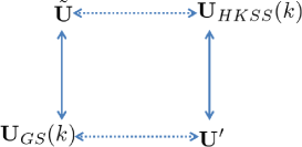
Figure 1: Spatial and temporal duality relationship of four quantum graph walks: The solid lines (vertical lines) depict the spatial reversal relationship in that ${\bf J}_{0}\tilde{{\bf U}}{\bf J}_{0}={\bf U}_{GS}(k)$ and ${\bf J}_{0}{\bf U}_{HKSS}(k){\bf J}_{0}={\bf U}^{\prime}$. The dotted lines (horizontal lines) express the temporal reversal relationship in that $\tilde{{\bf U}}^{-1}={\bf U}_{HKSS}(k)$ and ${\bf U}_{GS}(k)^{-1}={\bf U}^{\prime}$.

4 The characteristic polynomial of a scattering matrix of a quantum graph

Let $G$ be a connected graph with $n$ vertices and $m$ unoriented edges. Set $V(G)=\{1,2,\ldots,n\}$ and $D(G)=\{e_{1},e^{-1}_{1},\ldots,e_{m},e^{-1}_{m}\}$. Furthermore, for $j\in V(G)$ and $e\in D(G)$, let

$$x_{j}=\frac{2{\bf i}k}{{\bf i}kd_{j}-\lambda{}_{j}}\ and\ t_{e}=\exp{({\bf i}L_{e}(k-A_{e}))}.$$

Furthermore, set

$$\sigma^{(t(f))}_{ef}=\sigma^{(t(f))}_{ef}(k),{\bf U}={\bf U}(G)={\bf U}_{GS}(k),{\bf T}={\bf T}(k),{\bf S}={\bf S}(k).$$

Let an $n\times n$ matrix $\tilde{{\bf A}}=\tilde{{\bf A}}(\sigma{}^{2})=\tilde{{\bf A}}(G,\sigma{}^{2})=(\tilde{a}_{uv})$ be defined by

$$\tilde{a}_{uv}=\left\{\begin{array}[]{ll}\frac{x_{v}t_{e}}{\sigma{}^{2}-t_{e}t_{e^{-1}}}&\mbox{if $e=(u,v)\in D(G)$, }\\ 0&\mbox{otherwise.}\end{array}\right.\ \ \ \ \ \ \ (**)$$

Let an $n\times n$ matrix $\overline{{\bf A}}=\overline{{\bf A}}(\sigma{}^{2})=\overline{{\bf A}}(G,\sigma{}^{2})=(\overline{a}_{uv})$ be defined by

$$\overline{a}_{uv}=\left\{\begin{array}[]{ll}\frac{x_{u}t_{e}}{\sigma{}^{2}-t_{e}t_{e^{-1}}}&\mbox{if $e=(u,v)\in D(G)$, }\\ 0&\mbox{otherwise.}\end{array}\right.\ \ \ \ \ \ \ (***)$$

Furthermore, let an $n\times n$ diagonal matrix $\overline{{\bf D}}=\overline{{\bf D}}(\sigma{}^{2})=\overline{{\bf D}}(G,\sigma{}^{2})=(d_{uv})$ be defined by

$$d_{uv}=\left\{\begin{array}[]{ll}\sum_{o(e)=u}\frac{x_{u}t_{e}t_{e^{-1}}}{\sigma{}^{2}-t_{e}t_{e^{-1}}}&\mbox{if $u=v$, }\\ 0&\mbox{otherwise.}\end{array}\right.$$

Note that $t_{e}t_{e^{-1}}=1-e^{2ikL_{e}},e\in D(G)$.

Theorem 2.

Let $G$ be a connected graph with $n$ vertices and $m$ unoriented edges. Then

$$\det(\sigma{\bf I}_{2m}-{\bf U})=\det({\bf I}_{n}-\sigma\tilde{{\bf A}}+\overline{{\bf D}})\prod^{m}_{j=1}(\sigma{}^{2}-e^{2{\bf i}kL_{e_{j}}})=\det({\bf I}_{n}-\sigma\overline{{\bf A}}+\overline{{\bf D}})\prod^{m}_{j=1}(\sigma{}^{2}-e^{2{\bf i}kL_{e_{j}}}).$$

Proof. The argument is an analogue of the method of Watanabe and Fukumizu [40].

Let $D(G)=\{e_{1},\ldots,e_{m},e_{m+1},$ $\ldots,e_{2m}\}$ such that $e_{m+i}=e^{-1}_{i}(1\leq i\leq m)$. Furthermore, arrange arcs of $G$ as follows:

$$e_{1},e^{-1}_{1},\ldots,e_{m},e^{-1}_{m}.$$

Note that the $(e,f)$-array $({\bf U})_{ef}$ of ${\bf U}$ is given by

$$({\bf U})_{ef}=\left\{\begin{array}[]{ll}t_{e}(x_{o(e)}-\delta{}_{e^{-1}f})&\mbox{if $t(f)=o(e)$, }\\ 0&\mbox{otherwise.}\end{array}\right.$$

Let $2m\times 2m$ matrices ${\bf B}=({\bf B}_{ef})_{e,f\in D(G)}$ and ${\bf J}_{0}=({\bf J}_{ef})_{e,f\in D(G)}$ be defined as follows:

$${\bf B}_{ef}=\left\{\begin{array}[]{ll}x_{t(e)}&\mbox{if $t(e)=o(f)$, }\\ 0&\mbox{otherwise, }\end{array}\right.\ {\bf J}_{ef}=\left\{\begin{array}[]{ll}1&\mbox{if $f=e^{-1}$, }\\ 0&\mbox{otherwise.}\end{array}\right.$$

Note that ${}^{t}{\bf J}_{0}={\bf J}_{0}$.

Now

$${}^{t}{\bf S}={\bf B}-{\bf J}_{0}.$$ (31)

Let ${\bf K}=({\bf K}_{ev})$ _{e∈D(G);v∈V(G)} be the $2m\times n$ matrix defined as follows:

$${\bf K}_{ev}:=\left\{\begin{array}[]{ll}1&\mbox{if $o(e)=v$, }\\ 0&\mbox{otherwise. }\end{array}\right.$$

Furthermore, we define a $2m\times n$ matrix ${\bf L}=({\bf L}_{ev}){}_{e\in D(G);v\in V(G)}$ as follows:

$${\bf L}_{ev}:=\left\{\begin{array}[]{ll}1&\mbox{if $t(e)=v$, }\\ 0&\mbox{otherwise. }\end{array}\right.$$

Then we have

$${\bf L}{\bf X}{}^{t}{\bf K}={\bf B},$$ (32)

where

$${\bf X}=\left[\begin{array}[]{ccc}x_{1}&&0\\ &\ddots&\\ 0&&x_{n}\end{array}\right],$$

Next, By (31) and (32), we have

$$\begin{array}[]{rcl}&&\det({\bf I}_{2m}-s{\bf U})=\det({\bf I}_{2m}-s{\bf T}{\bf S})=\det({\bf I}_{2m}-s{\bf T}({}^{t}{\bf B}-{\bf J}_{0}))\\ &&\\ &=&\det({\bf I}_{2m}-s{\bf T}({\bf K}{\bf X}{}^{t}{\bf L}-{\bf J}_{0}))=\det({\bf I}_{2m}+s{\bf T}{\bf J}_{0}-s{\bf T}{\bf K}{\bf X}{}^{t}{\bf L})\\ &&\\ &=&\det({\bf I}_{2m}-s{\bf T}{\bf K}{\bf X}{}^{t}{\bf L}({\bf I}_{2m}+s{\bf T}{\bf J}_{0})^{-1})\det({\bf I}_{2m}+s{\bf T}{\bf J}_{0}).\end{array}$$

If ${\bf A}$ and ${\bf B}$ are a $m\times n$ and $n\times m$ matrices, respectively, then we have

$$\det({\bf I}_{m}-{\bf A}{\bf B})=\det({\bf I}_{n}-{\bf B}{\bf A}).$$ (33)

Thus, we have

$$\det({\bf I}_{2m}-s{\bf U})=\det({\bf I}_{2m}-s{\bf X}{}^{t}{\bf L}({\bf I}_{2m}+s{\bf T}{\bf J}_{0})^{-1}{\bf T}{\bf K})\det({\bf I}_{2m}+s{\bf T}{\bf J}_{0}).$$ (34)

Furthermore,

$$\det({\bf I}_{2m}-s{\bf U})=\det({\bf I}_{2m}-s{}^{t}{\bf L}({\bf I}_{2m}+s{\bf T}{\bf J}_{0})^{-1}{\bf T}{\bf K}{\bf X})\det({\bf I}_{2m}+s{\bf T}{\bf J}_{0}).$$ (35)

Next, we have

$${\bf I}_{2m}+s{\bf T}{\bf J}_{0}=\left[\begin{array}[]{ccccc}1&st_{e_{1}}&&&{\bf 0}\\ st_{e^{-1}_{1}}&1&&\\ &&\ddots&&\\ &&&1&st_{e_{m}}\\ {\bf 0}&&&st_{e^{-1}_{m}}&1\end{array}\right],$$

and so,

$$\det({\bf I}_{2m}+s{\bf T}{\bf J}_{0})=\prod^{m}_{j=1}(1-t_{e_{j}}t_{e^{-1}_{j}}s^{2}).$$

Furthermore, we have

$$({\bf I}_{2m}+s{\bf T}{\bf J}_{0})^{-1}=\left[\begin{array}[]{ccc}1/y_{1}&-st_{e_{1}}/y_{1}&{\bf 0}\\ -st_{e^{-1}_{1}}/y_{1}&1/y_{1}\\ {\bf 0}&&\ddots\end{array}\right],$$

where $y_{j}=1-t_{e_{j}}t_{e^{-1}_{j}}s^{2}\ (1\leq j\leq m)$.

For an arc $(u,v)\in D(G)$,

$$({\bf X}{}^{t}{\bf L}({\bf I}_{2m}+s{\bf T}{\bf J}_{0})^{-1}{\bf T}{\bf K})_{uv}=x_{u}t_{(v,u)}/(1-t_{(u,v)}t_{(v,u)}s^{2}).$$

Furthermore, if $u=v$, then

$$({\bf X}{}^{t}{\bf L}({\bf I}_{2m}+s{\bf T}{\bf J}_{0})^{-1}{\bf T}{\bf K})_{uu}=-\sum_{t(e)=u}\frac{x_{u}t_{e}t_{e^{-1}}s}{1-t_{e}t_{e^{-1}}s^{2}}.$$

Then we have

$${\bf X}{}^{t}{\bf L}({\bf I}_{2m}+s{\bf T}{\bf J}_{0})^{-1}{\bf T}{\bf K}=1/s^{2}\ {}^{t}\tilde{{\bf A}}(1/s^{2})-1/s\overline{{\bf D}}(1/s^{2}).$$

Therefore, by (34), it follows that

$$\begin{array}[]{rcl}&&\det({\bf I}_{2m}-s{\bf U})\\ &&\\ &=&\det({\bf I}_{n}-s{\bf X}{}^{t}{\bf L}({\bf I}_{2m}+s{\bf T}{\bf J}_{0})^{-1}{\bf T}{\bf K})\prod^{m}_{j=1}(1-t_{e_{j}}t_{e^{-1}_{j}}s^{2})\\ &&\\ &=&\det({\bf I}_{n}-1/s\ {}^{t}\tilde{{\bf A}}(1/s^{2})+\overline{{\bf D}}(1/s^{2}))\prod^{m}_{j=1}(1-t_{e_{j}}t_{e^{-1}_{j}}s^{2})\\ &&\\ &=&\det({\bf I}_{n}-1/s\tilde{{\bf A}}(1/s^{2})+\overline{{\bf D}}(1/s^{2}))\prod^{m}_{j=1}(1-t_{e_{j}}t_{e^{-1}_{j}}s^{2}).\end{array}$$

Next, for an arc $(u,v)\in D(G)$,

$$({}^{t}{\bf L}({\bf I}_{2m}+s{\bf T}{\bf J}_{0})^{-1}{\bf T}{\bf K}{\bf X})_{uv}=x_{v}t_{(v,u)}/(1-t_{(u,v)}t_{(v,u)}s^{2}).$$

Furthermore, if $u=v$, then

$$({\bf X}{}^{t}{\bf L}({\bf I}_{2m}+s{\bf T}{\bf J}_{0})^{-1}{\bf T}{\bf K}{\bf X})_{uu}=-\sum_{o(e)=u}\frac{x_{u}t_{e}t_{e^{-1}}s}{1-t_{e}t_{e^{-1}}s^{2}}.$$

Then we have

$${}^{t}{\bf L}({\bf I}_{2m}+s{\bf T}{\bf J}_{0})^{-1}{\bf T}{\bf K}{\bf X}=1/s^{2}\ {}^{t}\overline{{\bf A}}(1/s^{2})-1/s\overline{{\bf D}}(1/s^{2}).$$

Therefore, by (35), it follows that

$$\begin{array}[]{rcl}&&\det({\bf I}_{2m}-s{\bf U})\\ &&\\ &=&\det({\bf I}_{n}-s{}^{t}{\bf L}({\bf I}_{2m}+s{\bf T}{\bf J}_{0})^{-1}{\bf T}{\bf K}{\bf X})\prod^{m}_{j=1}(1-t_{e_{j}}t_{e^{-1}_{j}}s^{2})\\ &&\\ &=&\det({\bf I}_{n}-1/s\ {}^{t}\overline{{\bf A}}(1/s^{2})+\overline{{\bf D}}(1/s^{2}))\prod^{m}_{j=1}(1-t_{e_{j}}t_{e^{-1}_{j}}s^{2})\\ &&\\ &=&\det({\bf I}_{n}-1/s\overline{{\bf A}}(1/s^{2})+\overline{{\bf D}}(1/s^{2}))\prod^{m}_{j=1}(1-t_{e_{j}}t_{e^{-1}_{j}}s^{2}).\end{array}$$

Now, let $s=1/\sigma$. Then we get

$$\det\left({\bf I}_{2m}-\frac{1}{\sigma}{\bf U}\right)=\prod^{m}_{j=1}(1-t_{e_{j}}t_{e^{-1}_{j}}\frac{1}{\sigma{}^{2}})\det\left({\bf I}_{n}-\sigma\tilde{{\bf A}}(\sigma{}^{2})+\overline{{\bf D}}(\sigma{}^{2})\right).$$

Thus,

$$\det(\sigma{\bf I}_{2m}-{\bf U})=\prod^{m}_{j=1}(\sigma{}^{2}-t_{e_{j}}t_{e^{-1}_{j}})\det\left({\bf I}_{n}-\sigma\tilde{{\bf A}}(\sigma{}^{2})+\overline{{\bf D}}(\sigma{}^{2})\right).$$

Furthermore, we have

$$\det\left({\bf I}_{2m}-\frac{1}{\sigma}{\bf U}\right)=\prod^{m}_{j=1}(1-t_{e_{j}}t_{e^{-1}_{j}}\frac{1}{\sigma{}^{2}})\det\left({\bf I}_{n}-\sigma\overline{{\bf A}}(\sigma{}^{2})+\overline{{\bf D}}(\sigma{}^{2})\right).$$

Thus,

$$\det(\sigma{\bf I}_{2m}-{\bf U})=\prod^{m}_{j=1}(\sigma{}^{2}-t_{e_{j}}t_{e^{-1}_{j}})\det\left({\bf I}_{n}-\sigma\overline{{\bf A}}(\sigma{}^{2})+\overline{{\bf D}}(\sigma{}^{2})\right).$$

$\Box$

5 The characteristic polynomial of a scattering matrix of a regular covering of a graph

Let $G$ be a connected graph, and let $N(v)=\{w\in V(G)\mid(v,w)\in D(G)\}$ denote the neighbourhood of a vertex $v$ in $G$. A graph $H$ is a covering of $G$ with projection $\pi:H\longrightarrow G$ if there is a surjection $\pi:V(H)\longrightarrow V(G)$ such that $\pi{\mid}_{N(v^{\prime})}:N(v^{\prime})\longrightarrow N(v)$ is a bijection for all vertices $v\in V(G)$ and $v^{\prime}\in{\pi}^{-1}(v)$. When a finite group $\Pi$ acts on a graph $G$, the quotient graph $G/\Pi$ is a graph whose vertices are the $\Pi$-orbits on $V(G)$, with two vertices being adjacent in $G/\Pi$ if and only if some two of their representatives are adjacent in $G$. A covering $\pi:H\longrightarrow G$ is regular if there is a subgroup B of the automorphism group $Aut\ H$ of $H$ acting freely on $H$ such that the quotient graph $H/{\it B}$ is isomorphic to $G$.

Let $G$ be a graph and $\Gamma$ a finite group. Then a mapping $\alpha:D(G)\longrightarrow\Gamma$ is an ordinary voltage assignment if $\alpha(v,u)=\alpha(u,v)^{-1}$ for each $(u,v)\in D(G)$. The pair $(G,\alpha)$ is an ordinary voltage graph. The derived graph $G^{\alpha}$ of the ordinary voltage graph $(G,\alpha)$ is defined as follows: $V(G^{\alpha})=V(G)\times\Gamma$ and $((u,h),(v,k))\in D(G^{\alpha})$ if and only if $(u,v)\in D(G)$ and $k=h\alpha(u,v)$. The natural projection $\pi:G^{\alpha}\longrightarrow G$ is defined by $\pi(u,h)=u$. The graph $G^{\alpha}$ is a derived graph covering of $G$ with voltages in $\Gamma$ or a $\Gamma$-covering of $G$. The natural projection $\pi$ commutes with the right multiplication action of the $\alpha(e),e\in D(G)$ and the left action of $\Gamma$ on the fibers: $g(u,h)=(u,gh),g\in\Gamma$, which is free and transitive. Thus, the $\Gamma$-covering $G^{\alpha}$ is a $\mid\Gamma\mid$-fold regular covering of $G$ with covering transformation group $\Gamma$. Furthermore, every regular covering of a graph $G$ is a $\Gamma$-covering of $G$ for some group $\Gamma$ (see [10]). Figure 2 depicts the derived graph of $G=K_{3}$ with $\Gamma=\mathbb{Z}_{2}$.

Let $G$ be a connected graph, $\Gamma$ be a finite group and $\alpha:D(G)\longrightarrow\Gamma$ be an ordinary voltage assignment. In the $\Gamma$-covering $G^{\alpha}$, set $v_{g}=(v,g)$ and $e_{g}=(e,g)$, where $v\in V(G),e\in D(G),g\in\Gamma$. For $e=(u,v)\in D(G)$, the arc $e_{g}$ emanates from $u_{g}$ and terminates at $v_{g\alpha(e)}$. Note that $e^{-1}_{g}=(e^{-1})_{g\alpha(e)}$.

We consider the Gnutzmann-Smilansky type of the bond scattering matrix of the regular covering $G^{\alpha}$ of $G$. Let $V(G)=\{1,\ldots,n\}$, $D(G)=\{e_{1},\ldots,e_{m},e^{-1}_{1},\ldots,e^{-1}_{m}\}$ and $\Gamma=\{g_{1}=1,g_{2},\ldots,g_{p}\}$. Let $L:D(G)\longrightarrow{\bf R}^{+}$ and $A:D(G)\longrightarrow{\bf R}$ be the length and the magnetic flux of arcs of $G$. Let the length $\tilde{L}:D(G^{\alpha})\longrightarrow{\bf R}^{+}$ and the vector potential $\tilde{A}:D(G^{\alpha})\longrightarrow{\bf R}$ of arcs of $G^{\alpha}$ be given by

$$\tilde{L}_{e_{g}}=L_{e}\ and\ \tilde{A}_{e_{g}}=A_{e},e\in D(G),g\in\Gamma.$$

Let $e=(j,l)\in D(G)$. Then we consider the Schrödinger equation for the $e_{g}=(j_{g},l_{g\alpha(e)})$:

$$\left(-{\bf i}{\rm\frac{d}{dx}}+\tilde{A}_{e_{g}}\right)^{2}\Psi{}_{e_{g}}(x)=k^{2}\Psi{}_{e_{g}}(x)$$

under the following three conditions:

1. $\Psi{}_{e_{g}}(x)=\Psi{}_{e^{-1}_{g}}(\tilde{L}_{e_{g}}-x)$;

2. The continuity: $\Psi{}_{e_{g}}(0)=\phi{}_{j_{g}}$ and $\Psi{}_{e_{g}}(\tilde{L}_{e_{g}})=\phi{}_{l_{g\alpha(e)}}$;

3. The current conservation:

   $$\sum_{o(f_{g})=j_{g}}\left(-{\bf i}{\rm\frac{d}{dx}}+\tilde{A}_{f_{g}}\right)\Psi{}_{f_{g}}(x)\mid{}_{x=0}=-{\bf i}\lambda{}_{j_{g}}\phi{}_{j_{g}},\forall j_{g}\in V(G^{\alpha}),$$

   where $(\phi{}_{1,1},\ldots,\phi{}_{p,g_{m}})\in{\bf C}^{pm}$.

By the definitions of $\tilde{L}$ and $\tilde{A}$, the Schrödinger equation for the arc $e_{g}=(j_{g},l_{g\alpha(e)})$ and the three conditions 1,2,3 are reduced to the following system:

$$\left(-{\bf i}{\rm\frac{d}{dx}}+A_{e}\right)^{2}\Psi{}_{e_{g}}(x)=k^{2}\Psi{}_{e_{g}}(x)$$

and

1. $\Psi{}_{e_{g}}(x)=\Psi{}_{e^{-1}_{g}}(L_{e}-x)$;

2. $\Psi{}_{e_{g}}(0)=\phi{}_{j_{g}}$ and $\Psi{}_{e_{g}}(L_{e})=\phi{}_{l_{g\alpha(e)}}$;

3. $$\sum_{o(f_{g})=j_{g}}\left(-{\bf i}{\rm\frac{d}{dx}}+A_{f}\right)\Psi{}_{f_{g}}(x)\mid{}_{x=0}=-{\bf i}\lambda{}_{j_{g}}\phi{}_{j_{g}},\forall j_{g}\in V(G^{\alpha}).$$

The solution of the Schrödinger equation is given by

$$\Psi{}_{e_{g}}(x)=(c_{e^{-1}_{g}}e^{-{\bf i}kx}+b_{e_{g}}e^{{\bf i}kx})e^{-{\bf i}A_{e}x},{\bf i}=\sqrt{-1}.$$

Similarly to (9), we have

$$c_{e_{g}}=\sum_{t(f_{h})=j_{g}}\sigma{}^{(j_{g})}_{e_{g}f_{h}}e^{{\bf i}\tilde{L}_{e_{g}}(k-\tilde{A}_{e_{g}})}c_{f_{h}},$$

where

$$\sigma{}^{(j_{g})}_{e_{g}f_{h}}=\frac{2{\bf i}ik}{{\bf i}kd_{j_{g}}-\lambda{}_{j_{g}}}-\delta{}_{e^{-1}_{g}f_{h}}=\frac{2{\bf i}k}{{\bf i}kd_{j}-\lambda{}_{j_{g}}}-\delta{}_{e^{-1}_{g}f_{h}}.$$

Then the bond scattering matrix ${\bf U}(G^{\alpha})=(U(e_{g},f_{h}))_{e_{g},f_{h}\in D(G^{\alpha})}$ of $G^{\alpha}$ is given by

$$U(e_{g},f_{h})=\left\{\begin{array}[]{ll}t_{e_{g}}(x_{o(e_{g})}-\delta{}_{e^{-1}_{g}f_{h}})&\mbox{if $t(f_{h})=o(e_{g})$, }\\ 0&\mbox{otherwise,}\end{array}\right.$$ (36)

where

$$x_{v_{g}}=\frac{2{\bf i}k}{{\bf i}kd_{v}-\lambda{}_{v_{g}}}\ and\ t_{e_{g}}=e^{{\bf i}\tilde{L}_{e_{g}}(k-\tilde{A}_{e_{g}})}=e^{{\bf i}L_{e}(k-A_{e})}=t_{e}.$$

Now, we assume that

$$\lambda{}_{j_{g}}=\lambda{}_{j}\ for\ any\ j\in V(G)\ and\ g\in\Gamma.$$

Under this assumption, we have

$$x_{v_{g}}=\frac{2{\bf i}k}{{\bf i}kd_{v}-\lambda{}_{v}}=x_{v},\forall v\in V(G),\forall g\in\Gamma.$$

Then (36) is reduced to

$$U(e_{g},f_{h})=\left\{\begin{array}[]{ll}t_{e}(x_{o(e)}-\delta{}_{e^{-1}_{g}f_{h}})&\mbox{if $t(f_{h})=o(e_{g})$, }\\ 0&\mbox{otherwise.}\end{array}\right.$$

For $g\in\Gamma$, let the matrices $\tilde{{\bf A}}_{g}=\tilde{{\bf A}}_{g}(\sigma{}^{2})=(\tilde{a}^{(g)}_{uv})$ and $\overline{{\bf A}}_{g}=\overline{{\bf A}}_{g}(\sigma{}^{2})=(\overline{a}^{(g)}_{uv})$ be defined by

$$\tilde{a}^{(g)}_{uv}=\left\{\begin{array}[]{ll}\frac{x_{v}t_{e}}{\sigma{}^{2}-t_{e}t_{e^{-1}}}&\mbox{if $e=(u,v)\in D(G)$ and $\alpha(e)=g$, }\\ 0&\mbox{otherwise, }\end{array}\right.$$

$$\overline{a}^{(g)}_{uv}=\left\{\begin{array}[]{ll}\frac{x_{u}t_{e}}{\sigma{}^{2}-t_{e}t_{e^{-1}}}&\mbox{if $e=(u,v)\in D(G)$ and $\alpha(e)=g$, }\\ 0&\mbox{otherwise.}\end{array}\right.$$

Furthermore, let ${\bf U}_{g}=(U^{(g)}(e,f))$ be given by

$$U^{(g)}(e,f)=\left\{\begin{array}[]{ll}t_{e}(x_{o(e)}-\delta{}_{e^{-1}f})&\mbox{if $t(f)=o(e)$ and $\alpha(f)=g$, }\\ 0&\mbox{otherwise.}\end{array}\right.$$

Let ${\bf M}_{1}\oplus\cdots\oplus{\bf M}_{s}$ be the block diagonal sum of square matrices ${\bf M}_{1},\ldots,{\bf M}_{s}$. If ${\bf M}_{1}={\bf M}_{2}=\cdots={\bf M}_{s}={\bf M}$, then we write $s\circ{\bf M}={\bf M}_{1}\oplus\cdots\oplus{\bf M}_{s}$. The Kronecker product ${\bf A}\otimes{\bf B}$ of matrices A and B is considered as the matrix A having the element $a_{ij}$ replaced by the matrix $a_{ij}{\bf B}$.

Theorem 3.

Let $G$ be a connected graph with $n$ vertices and $m$ unoriented edges, $\Gamma$ be a finite group and $\alpha:D(G)\longrightarrow\Gamma$ be an ordinary voltage assignment. Assume that $\tilde{L}_{e_{g}}=L_{e}$, $\tilde{A}_{e_{g}}=A_{e}$ and $\lambda{}_{j_{g}}=\lambda{}_{j}$ for any $e\in D(G),j\in V(G),g\in\Gamma$. Set $|\Gamma|=p$. Furthermore, let ${\rho}_{1}=1,{\rho}_{2},\cdots,{\rho}_{k}$ be the irreducible representations of $\Gamma$, and $f_{i}$ be the degree of ${\rho}_{i}$ for each $i$, where $f_{1}=1$.

If the $\Gamma$-covering $G^{\alpha}$ of $G$ is connected, then, for the bond scattering matrix of $G{}^{\alpha}$,

$$\det(\sigma{\bf I}_{2mp}-{\bf U}(G^{\alpha}))=\det(\sigma{\bf I}_{2m}-{\bf U}(G))\prod^{k}_{i=2}\det(\sigma{\bf I}_{2mf_{i}}-\sum_{h\in\Gamma}{}^{t}{\rho}_{i}(h)\otimes{\bf U}{}_{h})^{f_{i}}$$

$$=\det({\bf I}_{n}-\sigma\overline{{\bf A}}+\overline{{\bf D}})\prod^{k}_{i=2}\det({\bf I}_{nf_{i}}-\sigma\sum_{h\in\Gamma}{\rho}_{i}(h)\otimes\overline{{\bf A}}{}_{h}+{\bf I}_{f_{i}}\otimes\overline{{\bf D}})^{f_{i}}\prod^{m}_{j=1}(\sigma{}^{2}-e^{2{\bf i}kL_{e_{j}}})^{p}.$$

$$=\det({\bf I}_{n}-\sigma\tilde{{\bf A}}+\overline{{\bf D}})\prod^{k}_{i=2}\det({\bf I}_{nf_{i}}-\sigma\sum_{h\in\Gamma}{\rho}_{i}(h)\otimes\tilde{{\bf A}}{}_{h}+{\bf I}_{f_{i}}\otimes\overline{{\bf D}})^{f_{i}}\prod^{m}_{j=1}(\sigma{}^{2}-e^{2{\bf i}kL_{e_{j}}})^{p},$$

where $D(G)=\{e_{1},e^{-1}_{1},\ldots,e_{m},e^{-1}_{m}\}$. Recall that $\tilde{{\bf A}}$ and $\overline{{\bf A}}$ is defined in (**) and (***), respectively.

Proof . Let $\mid\Gamma\mid=p$. By Theorem 2, we have

$$\det(\sigma{\bf I}_{2mp}-{\bf U}(G^{\alpha}))=\det({\bf I}_{np}-\sigma\overline{{\bf A}}(G^{\alpha},\sigma{}^{2})+\overline{{\bf D}}(G^{\alpha},\sigma{}^{2}))\prod^{m}_{j=1}(\sigma{}^{2}-t_{e_{j}}t_{e^{-1}_{j}})^{p}.$$

Let $D(G)=\{e_{1},\ldots,e_{m},e_{m+1},\ldots,e_{2m}\}$ such that $e_{m+j}=e^{-1}_{j}(1\leq j\leq m)$, and let $\Gamma=\{1=g_{1},g_{2},\ldots,g_{p}\}$. Arrange arcs of $G^{\alpha}$ in $p$ blocks: $(e_{1},1),\ldots,(e_{2m},1);(e_{1},g_{2}),\ldots,(e_{2m},g_{2})$; $\ldots;(e_{1},g_{p}),\ldots,(e_{2m},g_{p}).$ We consider the matrix ${\bf U}(G^{\alpha})$ under this order. For $h\in\Gamma$, the matrix ${\bf P}_{h}=(p^{(h)}_{ij})$ is defined as follows:

$$p^{(h)}_{ij}=\left\{\begin{array}[]{ll}1&\mbox{if $g_{i}h=g_{j}$,}\\ 0&\mbox{otherwise.}\end{array}\right.$$

Suppose that $p^{(h)}_{ij}=1$, i.e., $g_{j}=g_{i}h$. Then $U(e_{g_{i}},f_{g_{j}})\neq 0$ if and only if $t(f,g_{j})=o(e,g_{i})$. Furthermore, $t(f,g_{j})=o(e,g_{i})$ if and only if $(o(e),g_{i})=o(e,g_{i})=t(f,g_{j})=(t(f),g_{j}\alpha(f))$. Thus, $t(f)=o(e)$ and $\alpha(f)=g^{-1}_{j}g_{i}=g^{-1}_{j}g_{j}h^{-1}=h^{-1}$. Similarly, $(f,g_{j})=(e,g_{i})^{-1}$ if and only if $f=e^{-1}$ and $\alpha(f)=h^{-1}$. That is, under the assumption of (*),

$$U(e_{g},f_{h})=\left\{\begin{array}[]{ll}t_{e}(x_{o(e)}-\delta{}_{e^{-1}f})&\mbox{if $t(f)=o(e)$ and $\alpha(f)=h^{-1}$, }\\ 0&\mbox{otherwise.}\end{array}\right.$$

Now, by (36),

$${\bf U}(G^{\alpha})=\sum_{h\in\Gamma}{\bf P}_{h}\otimes{\bf U}{}_{h^{-1}}=\sum_{g\in\Gamma}{\bf P}_{g^{-1}}\otimes{\bf U}{}_{g}=\sum_{g\in\Gamma}{}^{t}{\bf P}_{g}\otimes{\bf U}{}_{g}.$$

Here, note that ${\bf P}_{g^{-1}}={}^{t}{\bf P}_{g}$ for each $g\in\Gamma$.

Let $\rho$ be the right regular representation of $\Gamma$. Furthermore, let ${\rho}_{1}=1,{\rho}_{2},\ldots,{\rho}_{k}$ be all inequivalent irreducible representations of $\Gamma$, and $f_{i}$ the degree of ${\rho}_{i}$ for each $i$, where $f_{1}=1$. Then we have $\rho(g)={\bf P}_{g}$ for $g\in\Gamma$. Furthermore, there exists a nonsingular matrix ${\bf P}$ such that ${\bf P}^{-1}\rho(g){\bf P}=(1)\oplus f_{2}\circ{\rho}_{2}(g)\oplus\cdots\oplus f_{k}\circ{\rho}_{k}(g)$ for each $g\in\Gamma$(see [30]). Thus, we have

$${}^{t}{\bf P}{}^{t}\rho(g){}^{t}{\bf P}^{-1}=(1)\oplus f_{2}\circ{}^{t}{\rho}_{2}(g)\oplus\cdots\oplus f_{k}\circ{}^{t}{\rho}_{k}(g).$$

Putting ${\bf F}=({}^{t}{\bf P}\otimes{\bf I}_{2q}){\bf U}(G^{\alpha})({}^{t}{\bf P}^{-1}\otimes{\bf I}_{2q})$, we have

$${\bf F}=\sum_{g\in\Gamma}\{(1)\oplus f_{2}\circ{}^{t}{\rho}_{2}(g)\oplus\cdots\oplus f_{k}\circ{}^{t}{\rho}_{k}(g)\}\otimes{\bf U}{}_{g}.$$

Note that ${\bf U}(G)=\sum_{g\in\Gamma}{\bf U}{}_{g}$ and $1+f^{2}_{2}+\cdots+f^{2}_{k}=p$. Therefore it follows that

$$\det(\sigma{\bf I}_{2mp}-{\bf U}(G^{\alpha}))=\det(\sigma{\bf I}_{2m}-{\bf U}(G))\prod^{k}_{i=2}\det(\sigma{\bf I}_{2mf_{i}}-\sum_{g}{}^{t}{\rho}_{i}(g)\otimes{\bf U}{}_{g})^{f_{i}}.$$

Next, let $V(G)=\{1,\ldots,n\}$. Arrange vertices of $G^{\alpha}$ in $p$ blocks: $(1,1),\ldots,(n,1);$ $(1,g_{2}),\ldots,(n,g_{2});\ldots;(1,g_{p}),\ldots,(n,g_{p}).$ We consider the matrix $\overline{{\bf A}}(G{}^{\alpha})$ defined in (***) under this order.

Suppose that $p^{(h)}_{ij}=1$, i.e., $g_{j}=g_{i}h$. Then $((u,g_{i}),(v,g_{j}))\in D(G{}^{\alpha})$ if and only if $(u,v)\in D(G)$ and $g_{j}=g_{i}\alpha(u,v)$. If $g_{j}=g_{i}\alpha(u,v)$, then $\alpha(u,v)=g^{-1}_{i}g_{j}=g^{-1}_{i}g_{i}h=h$. Thus we have

$$\overline{{\bf A}}(G{}^{\alpha})=\sum_{h\in\Gamma}{\bf P}_{h}\otimes\overline{{\bf A}}{}_{h}.$$

Putting ${\bf E}=({\bf P}^{-1}\otimes{\bf I}_{p})\overline{{\bf A}}(G{}^{\alpha})({\bf P}\otimes{\bf I}_{p})$ with nonsingular matrix ${\bf P}$, we have

$${\bf E}=\sum_{h\in\Gamma}\{(1)\oplus f_{2}\circ{\rho}_{2}(h)\oplus\cdots\oplus f_{k}\circ{\rho}_{k}(h)\}\otimes\overline{{\bf A}}{}_{h}.$$

Note that $\overline{{\bf A}}(G)=\sum_{h\in\Gamma}\overline{{\bf A}}{}_{h}$. Therefore it follows that

$$\begin{array}[]{rcl}\det({\bf I}_{np}-\sigma\overline{{\bf A}}(G^{\alpha},\sigma{}^{2})+\overline{{\bf D}}(G^{\alpha},\sigma{}^{2}))&=&\det({\bf I}_{n}-\sigma\overline{{\bf A}}+\overline{{\bf D}})\\ &&\\ &\times&\prod^{k}_{i=2}\det({\bf I}_{nf_{i}}-\sigma\sum_{h\in\Gamma}{\rho}_{i}(h)\otimes\overline{{\bf A}}{}_{h}+{\bf I}_{f_{i}}\otimes\overline{{\bf D}})^{f_{i}}.\end{array}$$

Hence, it follows that

$$\det(\sigma{\bf I}_{2mp}-{\bf U}(G^{\alpha}))=\det(\sigma{\bf I}_{2m}-{\bf U}(G))\prod^{k}_{i=2}\det(\sigma{\bf I}_{2mf_{i}}-\sum_{h}{}^{t}{\rho}_{i}(h)\otimes{\bf U}{}_{h})^{f_{i}}$$

$$=\det({\bf I}_{n}-\sigma\overline{{\bf A}}+\overline{{\bf D}})\prod^{k}_{i=2}\det({\bf I}_{nf_{i}}-\sigma\sum_{h\in\Gamma}{\rho}_{i}(h)\otimes\overline{{\bf A}}{}_{h}+{\bf I}_{f_{i}}\otimes\overline{{\bf D}})^{f_{i}}\prod^{m}_{j=1}(\sigma{}^{2}-e^{2{\bf i}kL_{e_{j}}})^{p}.$$

The third formula of Theorem is obtained similarly to the second one.

$\Box$

6 $L$-functions of graphs

We state a short review for the zeta function of a graph.

A path $P$ of length $n$ in $G$ is a sequence $P=(v_{0},e_{1},v_{1},e_{2},v_{2},\ldots,v_{n-1},e_{n},v_{n})$ of $n+1$ vertices and $n$ arcs such that $v_{0}\in V(G)$, $v_{i}\in V(G)$, $e_{i}\in D(G)$ and $e_{i}=(v_{i-1},v_{i})$ for $1\leq i\leq n$. We write $P=(e_{1},\ldots,e_{n})$. Set $|P|=n$, $o(P)=v_{0}$ and $t(P)=v_{n}$. Also, $P$ is called an $(o(P),t(P))$-path. We say that a path $P=(e_{1},\ldots,e_{n})$ has a backtracking if $e^{-1}_{i+1}=e_{i}$ for some $i$. A $(v,w)$-path is called a $v$-cycle (or $v$-closed path) if $v=w$. As standard terminologies of graph theory, a path and a cycle are a diwalk and a closed diwalk, respectively.

We introduce an equivalence relation on the set of cycles. Two cycles $C_{1}=(e_{1},\ldots,e_{m})$ and $C_{2}=(f_{1},\ldots,f_{m})$ are equivalent if there exists $k$ such that $f_{j}=e_{j+k}$ for all $j$. Let $[C]$ be the equivalence class that contains a cycle $C$. Let $B^{r}$ be the cycle obtained by going $r$ times around a cycle $B$. Such a cycle is called a power of $B$. A cycle $C$ is reduced if both $C$ and $C^{2}$ have no backtracking. Furthermore, a cycle $C$ is prime if it is not a power of a strictly smaller cycle. Note that each equivalence class of prime, reduced cycles of a graph $G$ corresponds to a unique conjugacy class of the fundamental group $\pi{}_{1}(G,v)$ of $G$ at a vertex $v$ of $G$.

The Ihara zeta function of a graph $G$ is defined to be a function of $u\in{\bf C}$ with $|u|$ sufficiently small, by

$${\bf Z}(G,u)={\bf Z}_{G}(u)=\prod_{[C]}(1-u^{\mid C\mid})^{-1},$$

where $[C]$ runs over all equivalence classes of prime, reduced cycles of $G$ (see [18]).

Theorem 4 (Bass).

If $G$ is a connected graph, then the reciprocal of the Ihara zeta function of $G$ is given by

$${\bf Z}(G,u)^{-1}=(1-u^{2})^{r-1}\det({\bf I}-u{\bf A}(G)+u^{2}({\bf D}-{\bf I})),$$

where $r$ and ${\bf A}(G)$ are the Betti number and the adjacency matrix of $G$, respectively, and ${\bf D}={\bf D}_{G}=(d_{ij})$ is the diagonal matrix with $d_{ii}=\deg v_{i}$ where $V(G)=\{v_{1},\ldots,v_{n}\}$.

Stark and Terras [33] gave an elementary proof of Theorem 4 and discussed three different zeta functions of any graph. Other proofs of Bass’ Theorem were given by Foata and Zeilberger [9] and Kotani and Sunada [23].

We introduce an $L$-function on the scattering matrix of a quantum graph. Let $G$ be a connected graph with $n$ vertices and $m$ unoriented edges, $\Gamma$ be a finite group and $\alpha:D(G)\longrightarrow\Gamma$ be an ordinary voltage assignment. Furthermore, let $\rho$ be a unitary representation of $\Gamma$ and $d$ its degree. We generalize the determinant of the second expression in Theorem 3. The $L$-function of $G$ associated with $\rho$ and $\alpha$ is defined by

$$\zeta{}_{G}(A,L,\lambda,\rho,\alpha,s)=\det({\bf I}_{2md}-s\sum_{h\in\Gamma}{}^{t}{\rho}(h)\otimes{\bf U}{}_{h})^{-1}.$$

If $\rho={\bf 1}$ is the identity representation of $\Gamma$, then the reciprocal of the $L$-function of $G$ is a determinant on the bond scattering matrix of $G$.

A determinant expression for the $L$-function of $G$ associated with $\rho$ and $\alpha$ is given as follows. For $1\leq i,j\leq n$, the $(i,j)$-block ${\bf F}_{i,j}$ of a $dn\times dn$ matrix ${\bf F}$ is the submatrix of ${\bf F}$ consisting of $d(i-1)+1,\ldots,di$ rows and $d(j-1)+1,\ldots,dj$ columns.

Theorem 5.

Let $G$ be a connected graph with $n$ vertices and $m$ unoriented edges, $\Gamma$ be a finite group and $\alpha:D(G)\longrightarrow\Gamma$ be an ordinary voltage assignment. If $\rho$ is a representation of $\Gamma$ and $d$ is the degree of $\rho$, then the reciprocal of the $L$-function of $G$ associated with $\rho$ and $\alpha$ is

$$\begin{array}[]{rcl}&&\zeta{}_{G}(A,L,\lambda,\rho,\alpha,s)^{-1}\\ &&\\ &=&\det({\bf I}_{nd}-s^{-1}\sum_{g\in\Gamma}\rho(g)\otimes\tilde{{\bf A}}_{g}(s^{-2})+{\bf I}_{d}\otimes\overline{{\bf D}}(s^{-2}))\prod^{m}_{j=1}(1-e^{2{\bf i}kL_{e_{j}}}s^{2})^{d}\\ &&\\ &=&\det({\bf I}_{nd}-s^{-1}\sum_{g\in\Gamma}\rho(g)\otimes\overline{{\bf A}}_{g}(s^{-2})+{\bf I}_{d}\otimes\overline{{\bf D}}(s^{-2}))\prod^{m}_{j=1}(1-e^{2{\bf i}kL_{e_{j}}}s^{2})^{d},\end{array}$$

where $D(G)=\{e_{1},e^{-1}_{1},\ldots,e_{m},e^{-1}_{m}\}$.

Proof. The argument is an analogue of the method of Watanabe and Fukumizu [40].

Let $D(G)=\{e_{1},\ldots,e_{m},e_{m+1},$ $\ldots,e_{2m}\}$ such that $e_{m+i}=e^{-1}_{i}(1\leq i\leq m)$. Furthermore, arrange arcs of $G$ as follows:

$$e_{1},e^{-1}_{1},\ldots,e_{m},e^{-1}_{m}.$$

Note that the $(e,f)$-block $(\sum_{g\in\Gamma}{\bf U}_{g}\otimes{}^{t}\rho(g))_{ef}$ of $\sum_{g\in\Gamma}{\bf U}_{g}\otimes{}^{t}\rho(g)$ is given by

$$(\sum_{g\in\Gamma}{\bf U}_{g}\bigotimes{}^{t}\rho(g))_{ef}=\left\{\begin{array}[]{ll}{}^{t}\rho(\alpha(f))t_{e}(x_{o(e)}-\delta{}_{e^{-1}f})&\mbox{if $t(f)=o(e)$, }\\ {\bf 0}_{d}&\mbox{otherwise.}\end{array}\right.$$

For $g\in\Gamma$, let the matrix ${\bf S}_{g}=(S^{(g)}_{ef})$ be defined by

$$S^{(g)}_{ef}=\left\{\begin{array}[]{ll}x_{o(e)}-\delta{}_{e^{-1}f}&\mbox{if $t(f)=o(e)$ and $\alpha(f)=g$, }\\ 0&\mbox{otherwise.}\end{array}\right.$$

Then we have

$$(\sum_{g\in\Gamma}{\bf U}_{g}\otimes{}^{t}\rho(g))=({\bf T}\otimes{\bf I}_{d})(\sum_{g\in\Gamma}{\bf S}_{g}\otimes{}^{t}\rho(g)).$$

For $g\in\Gamma$, two $2m\times 2m$ matrices ${\bf B}_{g}=({\bf B}^{(g)}_{ef})_{e,f\in D(G)}$ and ${\bf J}_{g}=({\bf J}^{(g)}_{ef})_{e,f\in D(G)}$ are defined as follows:

$${\bf B}^{(g)}_{ef}=\left\{\begin{array}[]{ll}x_{t(e)}&\mbox{if $t(e)=o(f)$ and $\alpha(e)=g$, }\\ 0&\mbox{otherwise}\end{array}\right.,{\bf J}^{(g)}_{ef}=\left\{\begin{array}[]{ll}1&\mbox{if $f=e^{-1}$ and $\alpha(e)=g$, }\\ 0&\mbox{otherwise.}\end{array}\right.$$

Now

$${}^{t}{\bf S}_{g}={\bf B}_{g}-{\bf J}_{g}\ for\ g\in\Gamma.$$

Let ${\bf K}=({\bf K}_{ev})$ _{e∈D(G);v∈V(G)} be the $2md\times nd$ matrix defined as follows:

$${\bf K}_{ev}:=\left\{\begin{array}[]{ll}{\bf I}_{d}&\mbox{if $o(e)=v$, }\\ {\bf 0}_{d}&\mbox{otherwise. }\end{array}\right.$$

Furthermore, we define a $2md\times nd$ matrix ${\bf L}=({\bf L}_{ev}){}_{e\in D(G);v\in V(G)}$ as follows:

$${\bf L}_{ev}:=\left\{\begin{array}[]{ll}\rho(\alpha(e))&\mbox{if $t(e)=v$, }\\ {\bf 0}_{d}&\mbox{otherwise. }\end{array}\right.$$

Then we have

$${\bf L}({\bf X}\otimes{\bf I}_{d}){}^{t}{\bf K}=\sum_{h\in\Gamma}{\bf B}{}_{h}\otimes\rho(h)={\bf B}_{\rho},$$ (37)

where

$${\bf B}_{\rho}=\sum_{g\in\Gamma}{\bf B}_{g}\otimes\rho(g).$$

Now, let

$${\bf X}_{d}={\bf X}\otimes{\bf I}_{d}\ and\ {\bf T}_{d}={\bf T}\otimes{\bf I}_{d}.$$

Then we have

$$\begin{array}[]{rcl}&&\det({\bf I}_{2md}-s\sum_{g\in\Gamma}{}^{t}\rho(g)\otimes{\bf U}_{g})=\det({\bf I}_{2md}-s\sum_{g\in\Gamma}{\bf U}_{g}\otimes{}^{t}\rho(g))\\ &&\\ &=&\det({\bf I}_{2md}-s{\bf T}_{d}(\sum_{g\in\Gamma}{\bf S}_{g}\otimes{}^{t}\rho(g))\\ &&\\ &=&\det({\bf I}_{2md}-s{\bf T}_{d}(\sum_{g\in\Gamma}{}^{t}{\bf B}_{g}\otimes{}^{t}\rho(g)-\sum_{g\in\Gamma}{}^{t}{\bf J}_{g}\otimes{}^{t}\rho(g)).\end{array}$$

Set

$${\bf J}_{\rho}=\sum_{g\in\Gamma}{\bf J}_{g}\otimes\rho(g).$$

Thus, by (37),

$$\begin{array}[]{rcl}&&\det({\bf I}_{2md}-s\sum_{g\in\Gamma}{}^{t}\rho(g)\otimes{\bf U}_{g})=\det({\bf I}_{2md}-s{\bf T}_{d}({\bf K}{\bf X}_{d}{}^{t}{\bf L}-{}^{t}{\bf J}_{\rho}))\\ &&\\ &=&\det({\bf I}_{2md}+s{\bf T}_{d}{}^{t}{\bf J}_{\rho}-s{\bf T}_{d}{\bf K}{\bf X}_{d}{}^{t}{\bf L})\\ &&\\ &=&\det({\bf I}_{2md}-s{\bf T}_{d}{\bf K}{\bf X}_{d}{}^{t}{\bf L}({\bf I}_{2md}+s{\bf T}_{d}{}^{t}{\bf J}_{\rho})^{-1})\det({\bf I}_{2md}+s{\bf T}_{d}{}^{t}{\bf J}_{\rho}).\end{array}$$

By (33), we have

$$\begin{array}[]{rcl}&&\det({\bf I}_{2md}-s\sum_{g\in\Gamma}{}^{t}\rho(g)\otimes{\bf U}_{g})\\ &&\\ &=&\det({\bf I}_{nd}-s{\bf X}_{d}{}^{t}{\bf L}({\bf I}_{2md}+s{\bf T}_{d}{}^{t}{\bf J}_{\rho})^{-1}{\bf T}_{d}{\bf K})\det({\bf I}_{2md}+s{\bf T}_{d}{}^{t}{\bf J}_{\rho}).\end{array}$$ (38)

Furthermore,

$$\begin{array}[]{rcl}&&\det({\bf I}_{2md}-s\sum_{g\in\Gamma}{}^{t}\rho(g)\otimes{\bf U}_{g})\\ &&\\ &=&\det({\bf I}_{nd}-s{}^{t}{\bf L}({\bf I}_{2md}+s{\bf T}_{d}{}^{t}{\bf J}_{\rho})^{-1}{\bf T}_{d}{\bf K}{\bf X}_{d})\det({\bf I}_{2md}+s{\bf T}_{d}{}^{t}{\bf J}_{\rho}).\end{array}$$ (39)

Next, we have

$${\bf I}_{2md}+s{\bf T}_{d}{}^{t}{\bf J}_{\rho}=\left[\begin{array}[]{ccccc}{\bf I}_{d}&st_{e_{1}}{}^{t}\rho(\alpha(e^{-1}_{1}))&&&{\bf 0}\\ st_{e^{-1}_{1}}{}^{t}\rho(\alpha(e_{1}))&{\bf I}_{d}&&\\ &&\ddots&&\\ &&&{\bf I}_{d}&st_{e_{m}}{}^{t}\rho(\alpha(e^{-1}_{m}))\\ {\bf 0}&&&st_{e^{-1}_{m}}{}^{t}\rho(\alpha(e_{m}))&{\bf I}_{d}\end{array}\right],$$

and so,

$$\det({\bf I}_{2md}+s{\bf T}_{d}{}^{t}{\bf J}_{\rho})=\prod^{m}_{j=1}(1-t_{e_{j}}t_{e^{-1}_{j}}s^{2})^{d}.$$

Furthermore, we have

$$({\bf I}_{2md}+s{\bf T}_{d}{}^{t}{\bf J}_{\rho})^{-1}=\left[\begin{array}[]{ccc}1/y_{1}{\bf I}_{d}&-st_{e_{1}}/y_{1}{}^{t}\rho(\alpha(e^{-1}_{1}))&{\bf 0}\\ -st_{e^{-1}_{1}}/y_{1}{}^{t}\rho(\alpha(e_{1}))&1/y_{1}{\bf I}_{d}&\\ {\bf 0}&&\ddots\end{array}\right],$$

where $y_{j}=1-t_{e_{j}}t_{e^{-1}_{j}}s^{2}\ (1\leq j\leq m)$.

For an arc $(u,v)\in D(G)$,

$$({\bf X}_{d}{}^{t}{\bf L}({\bf I}_{2md}+s{\bf T}_{d}{}^{t}{\bf J}_{\rho})^{-1}{\bf T}_{d}{\bf K})_{uv}=x_{u}t_{(v,u)}/(1-t_{(u,v)}t_{(v,u)}s^{2}){}^{t}\rho(\alpha(v,u)).$$

Furthermore, if $u=v$, then

$$({\bf X}_{d}{}^{t}{\bf L}({\bf I}_{2md}+s{\bf T}_{d}{}^{t}{\bf J}_{\rho})^{-1}{\bf T}_{d}{\bf K})_{uu}=-\sum_{t(e)=u}\frac{x_{u}t_{e}t_{e^{-1}}s}{1-t_{e}t_{e^{-1}}s^{2}}{\bf I}_{d}.$$

Then we have

$${\bf X}_{d}{}^{t}{\bf L}({\bf I}_{2md}+s{\bf T}_{d}{}^{t}{\bf J}_{\rho})^{-1}{\bf T}_{d}{\bf K}=1/s^{2}\sum_{g\in\Gamma}{}^{t}\tilde{{\bf A}}_{g}(1/s^{2})\otimes{}^{t}\rho(g)-1/s\overline{{\bf D}}(1/s^{2})\otimes{\bf I}_{d}.$$

By (38), it follows that

$$\begin{array}[]{rcl}&&\det({\bf I}_{2md}-s\sum_{g\in\Gamma}{}^{t}\rho(g)\otimes{\bf U}_{g})\\ &&\\ &=&\det({\bf I}_{nd}-s{\bf X}_{d}{}^{t}{\bf L}({\bf I}_{2md}+s{\bf T}_{d}{}^{t}{\bf J}_{\rho})^{-1}{\bf T}_{d}{\bf K})\prod^{m}_{j=1}(1-t_{e_{j}}t_{e^{-1}_{j}}s^{2})^{d}\\ &&\\ &=&\det({\bf I}_{nd}-1/s\sum_{g\in\Gamma}{}^{t}\tilde{{\bf A}}_{g}(1/s^{2})\otimes{}^{t}\rho(g)+\overline{{\bf D}}(1/s^{2})\otimes{\bf I}_{d})\prod^{m}_{j=1}(1-e^{2{\bf i}kL_{e_{j}}}s^{2})^{d}\\ &&\\ &=&\det({\bf I}_{nd}-1/s\sum_{g\in\Gamma}\tilde{{\bf A}}_{g}(1/s^{2})\otimes\rho(g)+\overline{{\bf D}}(1/s^{2})\otimes{\bf I}_{d})\prod^{m}_{j=1}(1-e^{2{\bf i}kL_{e_{j}}}s^{2})^{d}\\ &&\\ &=&\det({\bf I}_{nd}-1/s\sum_{g\in\Gamma}\rho(g)\otimes\tilde{{\bf A}}_{g}(1/s^{2})+{\bf I}_{d}\otimes\overline{{\bf D}}(1/s^{2}))\prod^{m}_{j=1}(1-e^{2{\bf i}kL_{e_{j}}}s^{2})^{d}.\end{array}$$

Next, for an arc $(u,v)\in D(G)$,

$$({}^{t}{\bf L}({\bf I}_{2md}+s{\bf T}_{d}{}^{t}{\bf J}_{\rho})^{-1}{\bf T}_{d}{\bf K}{\bf X}_{d})_{uv}=x_{v}t_{(v,u)}/(1-t_{(u,v)}t_{(v,u)}s^{2}){}^{t}\rho(\alpha(v,u)).$$

Furthermore, if $u=v$, then

$$({}^{t}{\bf L}({\bf I}_{2md}+s{\bf T}_{d}{}^{t}{\bf J}_{\rho})^{-1}{\bf T}_{d}{\bf K}{\bf X}_{d})_{uu}=-\sum_{o(e)=u}\frac{x_{u}t_{e}t_{e^{-1}}s}{1-t_{e}t_{e^{-1}}s^{2}}{\bf I}_{d}.$$

Then we have

$${}^{t}{\bf L}({\bf I}_{2md}+s{\bf T}_{d}{}^{t}{\bf J}_{\rho})^{-1}{\bf T}_{d}{\bf K}{\bf X}_{d}=1/s^{2}\sum_{g\in\Gamma}{}^{t}\overline{{\bf A}}_{g}(1/s^{2})\otimes{}^{t}\rho(g)-1/s\overline{{\bf D}}(1/s^{2})\otimes{\bf I}_{d}.$$

By (39), it follows that

$$\begin{array}[]{rcl}&&\det({\bf I}_{2md}-s\sum_{g\in\Gamma}{}^{t}\rho(g)\otimes{\bf U}_{g})\\ &&\\ &=&\det({\bf I}_{nd}-s{}^{t}{\bf L}({\bf I}_{2md}+s{\bf T}_{d}{}^{t}{\bf J}_{\rho})^{-1}{\bf T}_{d}{\bf K}{\bf X}_{d})\prod^{m}_{j=1}(1-t_{e_{j}}t_{e^{-1}_{j}}s^{2})^{d}\\ &&\\ &=&\det({\bf I}_{nd}-1/s\sum_{g\in\Gamma}{}^{t}\overline{{\bf A}}_{g}(1/s^{2})\otimes{}^{t}\rho(g)+\overline{{\bf D}}(1/s^{2})\otimes{\bf I}_{d})\prod^{m}_{j=1}(1-e^{2{\bf i}kL_{e_{j}}}s^{2})^{d}\\ &&\\ &=&\det({\bf I}_{nd}-1/s\sum_{g\in\Gamma}\overline{{\bf A}}_{g}(1/s^{2})\otimes\rho(g)+\overline{{\bf D}}(1/s^{2})\otimes{\bf I}_{d})\prod^{m}_{j=1}(1-e^{2{\bf i}kL_{e_{j}}}s^{2})^{d}\\ &&\\ &=&\det({\bf I}_{nd}-1/s\sum_{g\in\Gamma}\rho(g)\otimes\overline{{\bf A}}_{g}(1/s^{2})+{\bf I}_{d}\otimes\overline{{\bf D}}(1/s^{2}))\prod^{m}_{j=1}(1-e^{2{\bf i}kL_{e_{j}}}s^{2})^{d}.\end{array}$$

$\Box$

Thus,

Corollary 1.

Let $G$ be a connected graph with $n$ vertices and $m$ unoriented edges, $\Gamma$ be a finite group and $\alpha:D(G)\longrightarrow\Gamma$ be an ordinary voltage assignment. If $\rho$ is a irreducible representation of $\Gamma$ and $d$ is the degree of $\rho$, then

$$\begin{array}[]{rcl}&&\det(\sigma{\bf I}_{2md}-\sum_{h\in\Gamma}{}^{t}{\rho}_{i}(h)\otimes{\bf U}{}_{h})\\ &&\\ &=&\det({\bf I}_{nd}-\sigma\sum_{h\in\Gamma}{\rho}(h)\otimes\overline{{\bf A}}{}_{h}+{\bf I}_{d}\otimes\overline{{\bf D}})\prod^{m}_{j=1}(\sigma{}^{2}-e^{2{\bf i}kL_{e_{j}}})^{d}\\ &&\\ &=&\det({\bf I}_{nd}-\sigma\sum_{h\in\Gamma}{\rho}_{i}(h)\otimes\tilde{{\bf A}}{}_{h}+{\bf I}_{d}\otimes\overline{{\bf D}})\prod^{m}_{j=1}(\sigma{}^{2}-e^{2{\bf i}kL_{e_{j}}})^{d},\end{array}$$

where $D(G)=\{e_{1},e^{-1}_{1},\ldots,e_{m},e^{-1}_{m}\}$.

Proof. By Theorem 5, we have

$$\begin{array}[]{rcl}\\ &&\det(\sigma{\bf I}_{2mf_{i}}-\sum_{h\in\Gamma}{}^{t}{\rho}_{i}(h)\otimes{\bf U}{}_{h})=\sigma{}^{2md}\zeta{}_{G}(A,L,\lambda,\rho,\alpha,\sigma{}^{-1})^{-1}\\ &&\\ &=&\det({\bf I}_{nd}-\sigma\sum_{g\in\Gamma}\rho(g)\otimes\tilde{{\bf A}}_{g}(\sigma{}^{2})+{\bf I}_{d}\otimes\overline{{\bf D}}(\sigma{}^{2}))\prod^{m}_{j=1}(\sigma{}^{2}-e^{2{\bf i}kL_{e_{j}}})^{d}.\end{array}$$

$\Box$

By Theorem 5, it is also shown that, in Theorem 3, the determinant of the second expression is equal to that of the third expression.

By Theorem 3 and Corollary 1, the following result holds.

Corollary 2.

If $G$ is a connected graph with $m$ edges, $\Gamma$ is a finite group and $\alpha:D(G)\longrightarrow\Gamma$ is an ordinary voltage assignment, then we have

$$\det({\bf I}_{2mp}-{\bf U}(G^{\alpha}))=\sigma{}^{2mp}\prod_{\rho}\zeta{}_{G}(A,L,\lambda,\rho,\alpha,\sigma{}^{-1})^{-\deg\rho},$$

where $\rho$ runs over all inequivalent irreducible representations of $\Gamma$ and $p=\mid\Gamma\mid$.

7 The Euler product for the $L$-function $\zeta{}_{G}(A,L,\lambda,\rho,\alpha,s)$ of a graph

We present the Euler product for the $L$-function of a graph introduced in Section 6.

Foata and Zeilberger [9] gave a new proof of Bass’ Theorem by using the algebra of Lyndon words. Let $X$ be a finite nonempty set, $<$ a total order in $X$, and $X^{*}$ the free monoid generated by $X$. Then the total order $<$ on $X$ derives the lexicographic order $<^{*}$ on $X^{*}$. A Lyndon word in $X$ is defined to a nonempty word in $X^{*}$ that is prime (not the power $l^{r}$ of any other word $l$ for any $r\geq 2$) and that is also minimal in the class of its cyclic rearrangements under $<^{*}$ (see [26]). Let $L$ denote the set of all Lyndon words in $X$.

Foata and Zeilberger [9] gave a short proof of Amitsur’s identity [3].

Theorem 6 (Amitsur).

For square matrices ${\bf A}_{1},\ldots,{\bf A}_{k}$,

$$\det({\bf I}-({\bf A}_{1}+\cdots+{\bf A}_{k}))=\prod_{l\in L}\det({\bf I}-{\bf A}_{l}),$$

where the product runs over all Lyndon words in $\{1,\cdots,k\}$, and ${\bf A}_{l}={\bf A}_{i_{1}}\cdots{\bf A}_{i_{r}}$ for $l=i_{1}\cdots i_{r}$.

Theorem 7.

Let $G$ be a connected graph with $n$ vertices and $m$ unoriented edges, $\Gamma$ be a finite group and $\alpha:D(G)\longrightarrow\Gamma$ be an ordinary voltage assignment. For each path $P=(e_{1},\ldots,e_{p})$ of $G$, set $\alpha(P)=\alpha(e_{1})\cdots\alpha(e_{p})$. If $\rho$ is a representation of $\Gamma$ and $d$ is the degree of $\rho$, then

$$\zeta{}_{G}(A,L,\lambda,\rho,\alpha,s)=\prod_{[C]}\det({\bf I}_{d}-{}^{t}\rho(\alpha(C))t_{C}a_{C}s^{|C|})^{-1},$$

where $[C]$ runs over all equivalence classes of prime cycles of $G$, and

$$t_{C}=t_{e_{1}}\cdots t_{e_{p}},a_{C}=\sigma{}^{(o(e_{1}))}_{e_{1}e_{p}}\sigma{}^{(o(e_{p}))}_{e_{p}e_{p-1}}\cdots\sigma{}^{(o(e_{2}))}_{e_{2}e_{1}},\ C=(e_{1},e_{2},\ldots,e_{p})$$

Proof. At first, let $D(G)=\{e_{1},\ldots,e_{m},e_{m+1},\ldots,e_{2m}\}$ and consider the lexicographic order on $D(G)\times D(G)$ derived from a total order of $D(G)$: $e_{1}<e_{2}<\cdots<e_{2m}$. If $(e_{i},e_{j})$ is the $c$-th pair under the above order, then we define the $2md\times 2md$ matrix ${\bf T}_{c}=(({\bf T}_{c}){}_{r,s})_{1\leq r,s\leq 2m}$ as follows:

$$({\bf T}_{c})_{r,s}=\left\{\begin{array}[]{ll}{}^{t}\rho(\alpha(e_{j}))t_{e_{i}}\sigma{}^{(o(e_{i}))}_{e_{i}e_{j}}&\mbox{if $r=e_{i},s=e_{j}$ and $o(e_{i})=t(e_{j})$, }\\ {\bf 0}&\mbox{otherwise, }\end{array}\right.$$

where

$$\sigma{}^{(o(e))}_{ef}=x_{o(e)}-\delta{}_{e^{-1}f}.$$

If ${\bf F}={\bf T}_{1}+\cdots+{\bf T}_{k}$ and $k=4m^{2}$, then

$${\bf F}=\sum_{h\in\Gamma}{\bf U}{}_{h}\otimes{}^{t}\rho(h).$$

Let $L$ be the set of all Lyndon words in $D(G)\times D(G)$. We can also consider $L$ as the set of all Lyndon words in $\{1,\ldots,k\}$: $(e_{i_{1}},e_{j_{1}})\cdots(e_{i_{s}},e_{j_{s}})$ corresponds to $m_{1}m_{2}\cdots m_{s}$, where $(e_{i_{r}},e_{j_{r}})(1\leq r\leq s)$ is the $m_{r}$-th pair. Theorem 6 implies that

$$\det({\bf I}_{2qd}-s{\bf F})=\prod_{t\in L}\det({\bf I}_{2md}-s^{|l|}{\bf T}_{l}),$$

where

$${\bf T}_{l}={\bf T}_{i_{1}}\cdots{\bf T}_{i_{r}}$$

for $l=i_{1}\cdots i_{r}$. Note that $\det({\bf I}_{2md}-s^{|l|}{\bf T}_{l})$ is the alternating sum of the diagonal minors of ${\bf T}_{l}$. Thus, we have

$$\det({\bf I}-s^{|t|}{\bf T}_{t})=\left\{\begin{array}[]{ll}\det({\bf I}-{}^{t}\rho(\alpha(C))t_{C}a_{C}s^{|C|})&\mbox{if $t$ is a prime cycle $C$, }\\ 1&\mbox{otherwise, }\end{array}\right.$$

where

$$t_{C}=t_{e_{1}}\cdots t_{e_{p}},a_{C}=\sigma{}^{(o(e_{1}))}_{e_{1}e_{p}}\sigma{}^{(o(e_{p}))}_{e_{p}e_{p-1}}\cdots\sigma{}^{(o(e_{2}))}_{e_{2}e_{1}},\ C=(e_{1},e_{2},\ldots,e_{p})$$

Therefore, it follows that

$$\zeta{}_{G}(A,L,\lambda,\rho,\alpha,s)^{-1}=\det({\bf I}_{2md}-s\sum_{h\in\Gamma}{}^{t}\rho(h)\otimes{\bf U}{}_{h})$$

$$=\det({\bf I}_{2md}-s\sum_{h\in\Gamma}{\bf U}{}_{h}\otimes{}^{t}\rho(h))=\prod_{[C]}({\bf I}_{d}-{}^{t}\rho(\alpha(C))t_{C}a_{C}s^{|C|}),$$

where $[C]$ runs over all equivalence classes of prime cycles of $G$.

$\Box$

8 Example

We give an example. See also Fig. 2, Let $G=K_{3}$ be the complete graph with three vertices $v_{1},v_{2},v_{3}$ and six arcs $e_{1},e_{2},e_{3},e^{-1}_{1},e^{-1}_{2},e^{-1}_{3}$, where $e_{1}=(v_{1},v_{2}),e_{2}=(v_{2},v_{3}),e_{3}=(v_{3},v_{1})$. Furthermore, let $\lambda{}_{v}=\lambda$ for $v\in V(G)$, $L_{e}=L,A_{e}=A$ for any $e\in D(G)$. Then we have

$$x_{v_{j}}=\frac{2{\bf i}k}{2{\bf i}k-\lambda},t_{e_{j}}=\exp({\bf i}L(k-A)),t_{e^{-1}_{j}}=\exp({\bf i}L(k+A))\ (j=1,2,3).$$

Set $a=\frac{2{\bf i}k}{2{\bf i}k-\lambda}$, $t=\exp({\bf i}L(k-A))$ and $s=\exp({\bf i}L(k+A))$. Considering ${\bf U}$ under the order $e_{1},e_{2},e_{3},e^{-1}_{1},e^{-1}_{2},e^{-1}_{3}$, we have

$${\bf U}={\bf U}_{GS}=\left[\begin{array}[]{cccccc}0&0&ta&t(a-1)&0&0\\ ta&0&0&0&t(a-1)&0\\ 0&ta&0&0&0&t(a-1)\\ s(a-1)&0&0&0&sa&0\\ 0&s(a-1)&0&0&0&sa\\ 0&0&s(a-1)&sa&0&0\end{array}\right]$$

and

$$\tilde{{\bf A}}=\overline{{\bf A}}=\frac{a}{\sigma{}^{2}-st}\left[\begin{array}[]{ccc}0&t&s\\ s&0&t\\ t&s&0\end{array}\right],{\bf D}=\frac{2ast}{\sigma{}^{2}-st}{\bf I}_{3}.$$

By Theorem 2, we have

$$\det(\sigma{\bf I}_{6}-{\bf U})=(\sigma{}^{2}-st)^{3}\det({\bf I}_{3}-\sigma\overline{{\bf A}}+\overline{{\bf D}})=\det\left[\begin{array}[]{ccc}b&-ta\sigma&-sa\sigma\\ -sa\sigma&b&-ta\sigma\\ -ta\sigma&-sa\sigma&b\end{array}\right]$$

$$=b(b^{2}-3sta^{2}\sigma{}^{2})-a^{3}\sigma{}^{3}(s^{3}+t^{3}).$$

where $b=\sigma{}^{2}+(2a-1)st$.

Next, let $\Gamma=Z_{2}=\{1,-1\}$ be the cyclic group of order 2, and let $\alpha:D(K_{3})\longrightarrow Z_{2}$ be the ordinary voltage assignment such that $\alpha(e_{1})=\alpha(e^{-1}_{1})=-1$ and $\alpha(e_{2})=\alpha(e^{-1}_{2})=\alpha(e_{3})=\alpha(e^{-1}_{3})=1$. The characters of ${\bf Z}_{2}$ are given as follows: $\chi{}_{i}((-1)^{j})=((-1)^{i})^{j}$, $0\leq i,j\leq 1$. Then we have

$$\overline{{\bf A}}_{1}=\frac{a}{\sigma{}^{2}-st}\left[\begin{array}[]{ccc}0&0&s\\ 0&0&t\\ t&s&0\end{array}\right],\overline{{\bf A}}_{-1}=\frac{a}{\sigma{}^{2}-st}\left[\begin{array}[]{ccc}0&-s&0\\ -s&0&0\\ 0&0&0\end{array}\right].$$

Now, by Theorem 5,

$$\begin{array}[]{rcl}\sigma{}^{6}{\zeta}_{K_{3}}(A,L,\lambda,\chi{}_{1},\alpha,\sigma{}^{-2})^{-1}&=&(\sigma{}^{2}-st)^{3}\det({\bf I}_{3}-\sigma\sum^{1}_{i=0}\chi((-1)^{i})\overline{{\bf A}}_{(-1)^{i}}+\overline{{\bf D}})\\ &&\\ &=&\det\left[\begin{array}[]{ccc}b&ta\sigma&-sa\sigma\\ sa\sigma&b&-ta\sigma\\ -ta\sigma&-sa\sigma&b\end{array}\right]\\ &&\\ &=&b(b^{2}-3sta^{2}\sigma{}^{2})+a^{3}\sigma{}^{3}(s^{3}+t^{3}).\end{array}$$

By Corollary 2, it follows that

$$\begin{array}[]{rcl}&&\det(\sigma{\bf I}_{12}-{\bf U}(K^{\alpha}_{3}))=\det({\sigma{}^{2}\bf I}_{6}-{\bf U})\zeta{}_{K_{3}}(A,L,\lambda,\chi,\alpha,\sigma{}^{-2})^{-1}\sigma{}^{6}\\ &&\\ &=&\{b(b^{2}-3sta^{2}\sigma{}^{2})-a^{3}\sigma{}^{3}(s^{3}+t^{3})\}\{b(b^{2}-3sta^{2}\sigma{}^{2})+a^{3}\sigma{}^{3}(s^{3}+t^{3})\}\\ &&\\ &=&b^{2}(b^{2}-3sta^{2}\sigma{}^{2})^{2}-a^{6}\sigma{}^{6}(s^{3}+t^{3})^{2}.\end{array}$$

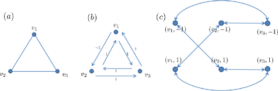
Figure 2: Regular covering of $G=K_{3}$: Figure (a) is the original graph $G=K_{3}$. We take $\Gamma=\mathbb{Z}_{2}=\{-1,1\}$. As an ordinary assignment $\alpha$, we assign elements of $\Gamma$ to arcs as is depicted by Fig. (b). For example, $\alpha(1,2)=-1$, $\alpha(2,3)=1$. The definition of the assignment imposes $\alpha(2,1)=-1$, $\alpha(3,2)=1$ since $\alpha(v,u)=\alpha(u,v)^{-1}$ for any $(u,v)\in D(G)$. Figure (c) is the derived graph $G^{\alpha}$. For example, putting $e=(v_{1},v_{2})\in D(G)$, then, for $\pm 1\in\Gamma$, $e_{1}=((v_{1},1),(v_{2},-1))\in D(G^{\alpha})$ and $e_{-1}=((v_{1},-1),(v_{2},1))\in D(G^{\alpha})$ since $((u,g),(v,h))\in D(G^{\alpha})$ if and only if $(u,v)\in D(G)$ and $h=g\alpha(u,v)$, in this case, $-1=\alpha(v_{1},v_{2})\times 1$ and $1=\alpha(v_{1},v_{2})\times(-1)$, respectively.

Acknowledgments.

The first author was supported in part by the Grant-in-Aid for Scientific Research (C) 20540133 and (B) 24340031 from Japan Society for the Promotion of Science. The second and third authors also acknowledge financial supports of the Grant-in- Aid for Scientific Research (C) from Japan Society for the Promotion of Science (Grant No. 24540116 and No. 23540176, respectively).

References

[1]
[2]A. Ambainis,
Quantum walks and their algorithmic applications,
International Journal of Quantum Information 1 (2003), 507–518
[3]
[4]A. Ambainis, E. Bach, A. Nayak, A. Vishwanath, and J. Watrous:
One-dimensional quantum walks,
Proc. 33rd Annual ACM Symp. Theory of Computing, (2001), 37–49.
[5]
[6]S. A. Amitsur,
On the characteristic polynomial of a sum of matrices,
Linear and Multilinear Algebra 8 (1980), 177-182.
[7]
[8]H. Bass,
The Ihara-Selberg zeta function of a tree lattice,
Internat. J. Math. 3 (1992), 717-797.
[9]
[10]A. Comtet, J. Desbois and C. Texier,
Functionals of the Brownian motion, localization and metric graphs,
J. Phys. A: Math. Gen. 38 (2005), R341-R383.
[11]
[12]J. Desbois,
Spectral determinant on graphs with generalized boundary conditions,
Eur. Phys. J. B 24 (2001), 261-266.
[13]
[14]D. Emms, E. R. Hancock, S. Severini, R. C. Wilson,
A matrix representation of graphs and its spectrum as a graph invariant,
Electr. J. Combin. 13 (2006), R34.
[15]
[16]P. Exner, P. Šeba,
Free quantum motion on a branching graph,
Rep. Math. Phys. 28 (1989), 7-26.
[17]
[18]D. Foata and D. Zeilberger,
A combinatorial proof of Bass’s evaluations of the Ihara-Selberg zeta
function for graphs,
Trans. Amer. Math. Soc. 351 (1999), 2257-2274.
[19]
[20]J. L. Gross and T. W. Tucker,
Topological Graph Theory,
Wiley-Interscience, New York, 1987.
[21]
[22]S. Gnutzmann and U. Smilansky,
Quantum graphs: Applications to quantum chaos and universal
spectral statistics,
Advances in Physics 55 (2006), 527-625.
[23]
[24]S. Gudder,
Quantum Probability,
Academic Press Inc., CA, (1988).
[25]
[26]J. M. Harrison and K. Kirsten,
Zeta functions of quantum graphs,
J. Phys. A: Math. Theor. 44 (2011), 235301, 29 pp.
[27]
[28]J. M. Harrison, U. Smilansky and B. Winn,
Quantum graphs where back-scattering is prhibited,
J. Phys. A:Math. Theor. 40 (2007), 14181-14193.
[29]
[30]K. Hashimoto,
Zeta Functions of Finite Graphs and Representations
of -Adic Groups,
in ”Adv. Stud. Pure Math”. Vol. 15, pp. 211-280, Academic Press,
New York, 1989.
[31]
[32]Yu. Higuchi, N. Konno, I. Sato and E. Segawa,
Quantum graph walks I: mapping to quantum graphs,
arXiv:1211.0803.
[33]
[34]Yu. Higuchi, N. Konno, I. Sato, and E. Segawa,
Quantum graph walks III: scattering operator via discrete laplacian,
in preparation.
[35]
[36]Y. Ihara,
On discrete subgroups of the two by two projective linear group
over -adic fields,
J. Math. Soc. Japan 18 (1966), 219-235.
[37]
[38]J. Kempe,
Quantum random walks - an introductory overview,
Contemporary Physics 44 (2003), 307–327.
[39]
[40]V. Kendon,
Decoherence in quantum walks - a review,
Math. Struct. in Comp. Sci. 17 (2007), 1169–1220.
[41]
[42]N. Konno,