Magnetic Cluster Excitations

Abstract

Magnetic clusters, i.e., assemblies of a finite number (between two or three and several hundred) of interacting spin centers which are magnetically decoupled from their environment, can be found in many materials ranging from inorganic compounds, magnetic molecules, artificial metal structures formed on surfaces to metalloproteins. The magnetic excitation spectra in them are determined by the nature of the spin centers, the nature of the magnetic interactions, and the particular arrangement of the mutual interaction paths between the spin centers. Small clusters of up to four magnetic ions are ideal model systems to examine the fundamental magnetic interactions which are usually dominated by Heisenberg exchange, but often complemented by anisotropic and/or higher-order interactions. In large magnetic clusters which may potentially deal with a dozen or more spin centers, the possibility of novel many-body quantum states and quantum phenomena are in focus. In this review the necessary theoretical concepts and experimental techniques to study the magnetic cluster excitations and the resulting characteristic magnetic properties are introduced, followed by examples of small clusters demonstrating the enormous amount of detailed physical information which can be retrieved. The current understanding of the excitations and their physical interpretation in the molecular nanomagnets which represent large magnetic clusters is then presented, with an own section devoted to the subclass of the single-molecule magnets which are distinguished by displaying quantum tunneling of the magnetization. Finally, some quantum many-body states are summarized which evolve in magnetic insulators characterized by built-in or field-induced magnetic clusters. The review concludes addressing future perspectives in the field of magnetic cluster excitations.

I Introduction

Magnetic clusters are defined as systems which consist of a finite number $N$ of interacting spins that are magnetically isolated from the environment, where the number $N$ may be as small as two or can be several hundreds. Larger entities of thousands to a few millions of atoms, which are usually referred to as nanoscale or ultrafine particles, are excluded from the present review. Magnetic clusters either occur naturally in pure compounds, where the magnetic isolation of the clusters is provided by nonmagnetic ligands, or are formed artificially, e.g., in solid solutions of magnetic and nonmagnetic compounds. Prototypes of pure compounds are molecular nanomagnets in which a polynuclear magnetic metal core is embedded in a diamagnetic ligand matrix. Examples associated with cooperative systems are diluted magnetic compounds, in which the magnetic ions are randomly distributed, so that different types of magnetic clusters ($N$-mers, $N=1,2,3,\ldots$) are simultaneously present.

Many of the characteristic physical properties of magnetic clusters are determined by the magnetic excitation spectra which reflect the nature of the fundamental magnetic interactions between the spins in a cluster. The latter can be quantitatively accounted for by a spin Hamiltonian in which a bilinear Heisenberg-type exchange interaction is usually the dominant term, often complemented by additional terms describing the anisotropic and/or higher-order interactions. As long as the number $N$ of spins is reasonably small, exact analytical solutions of the spin Hamiltonian can be obtained. Accordingly, small magnetic clusters are ideal model systems to explore experimentally the limitations of the theoretical models. However, the synthesis strategies to produce molecular magnetic materials have advanced enormously in recent years, making available bounded molecular magnetic clusters with the number $N$ of magnetic centers varying from one to several dozens; the record currently stands at $N=84$ in the torus-like molecule Mn₈₄ Tasiopoulos et al. (2004). In this new class of magnetic materials, now commonly called molecular nanomagnets Gatteschi et al. (2006b), clusters with more than four metal ions are rather the rule than the exception, shifting the main scientific challenge away from that of studying the nature of the basic interactions towards that of exploring the possible consequences of having such interactions in a lattice of exchange-coupled spin centers.

In the past decade, magnetic cluster systems have become a topic of increasing interest and relevance in condensed matter science. They are not only interesting in themselves for determining the origin and the size of the fundamental magnetic interactions, but they have also important applications in both technology and science. Molecular nanomagnets are currently considered among the most promising candidates as the smallest nanomagnetic units capable of storing and processing quantum information Troiani et al. (2005). In particular, magnetic molecules with large spin ground states and negative axial anisotropy or single-molecule magnets were found to exhibit outstanding properties such as slow relaxation of the magnetization and stepped magnetic hysteresis curves due to quantum tunneling of the magnetization at low temperatures Christou et al. (2000); Gatteschi and Sessoli (2003); Chudnovsky and Tejada (1998).

Another emerging field concerns transition-metal perovskites in which magnetic polarons evolve upon hole doping and behave like magnetic nanoparticles embedded in a nonmagnetic matrix Phelan et al. (2006). Furthermore, we mention the remarkable observations of quantum phase transitions, Bose-Einstein condensation and field-induced three-dimensional magnetic ordering in weakly interacting antiferromagnetic dimer compounds Sachdev (1999); Giamarchi et al. (2008) as well as the attractive phenomenon of spin-Peierls dimerization in both organic and inorganic compounds Bray et al. (1975). Very recently, magnetic cluster systems could also be fabricated directly on surfaces using scanning microscope techniques Hirjibehedin et al. (2006). Even in biology, magnetic metal clusters are important subunits. Polynuclear iron clusters are contained in proteins like adrenodoxin and ferredoxin, which are involved in the photosynthetic process to convert light energy into chemical energy based on electron transfer mechanisms Griffith (1972). All these systems have a common property, namely the presence of magnetic clusters, whose characterization is therefore a key issue in both theoretical and experimental investigations.

An important class of magnetic cluster systems concerns magnetic nanoparticles containing a few hundreds of atoms produced by e.g. sputtering, inert-gas condensation techniques, direct ball milling or microemulsion-based syntheses. In principle, the spin dynamics exhibits many features similar to the molecular nanomagnets, such as superparamagnetic relaxation and quantized spin-wave states. Pioneering neutron scattering experiments in this area have been performed for Fe nanoparticles Hennion et al. (1994) and for nanocrystallites of hematite Kuhn et al. (2006); Hansen et al. (1997). In practice, the interpretation of experimental data on magnetic nanoparticles is made difficult by line broadening effects due to variations in size and form, and the presence of a variety of surface spin states. Any discussion of the magnetic properties needs considering these aspects, and for that reason the magnetic nanoparticles are excluded from the present review, in particular as excellent reviews of the theoretical and experimental aspects exist Hendriksen et al. (1993); Kodama (1999).

Our main objective in this review is to introduce the theoretical concepts and the experimental techniques applied to the study of magnetic cluster excitations as well as to give a snapshot of recent developments achieved for the most important classes of materials whose properties are largely governed by the presence of magnetic clusters. The outline of this review is as follows: Sec. II starts with a summary of the basic terms of the underlying spin Hamiltonians and with a short description of the most powerful experimental techniques, followed by representative examples on small magnetic clusters (dimers, trimers, and tetramers) in Sec. III to demonstrate the enormous amount of detailed physical information resulting from the study of magnetic cluster excitations. Clusters with a small number $N$ of coupled magnetic ions are excellent choices for this purpose, as the basic interactions are all present in them and can be treated exactly, hence a straightforward comparison between theory and experiment is possible with little ambiguity. This is no longer the case for the emerging field of large magnetic clusters discussed in Sec. IV, in which the number $N$ of magnetic centers can be as large as several dozens, so that the interpretation and analysis of the experimental results require the use of sophisticated tools. In addition, novel physical aspects such as complex many-body quantum states come into play as a consequence of the large cluster size. An important subclass of the large magnetic clusters will be addressed in Sec. V, namely the single-molecule magnets in which at low temperatures magnetic hysteresis or slow magnetic relaxation and quantum tunneling of the magnetization can be observed. Many methodologies applied to the large magnetic clusters have their origin in the field of quantum spin systems which are summarized in Sec. VI for cases where the presence of magnetic clusters is the most important ingredient to understand their quantum spin properties. We conclude with a brief outlook in Sec. VII. Given the abundant literature on the topic of magnetic cluster excitations, the present review is necessarily bound to be incomplete in terms of both materials covered and references cited. The experimental results were chosen according to their didactical suitability to illustrate the concepts, including both historical data from the pioneering time and data of today’s research.

II Basics

II.1 Spin Hamiltonian

The form of the appropriate spin Hamiltonian of magnetic cluster systems depends on two essentially independent terms: the nature of the interacting systems in the absence of interactions, and the physical nature of the mechanisms responsible for the interactions Wolf (1971). The total Hamiltonian describing interacting spins can generally be written as

$$\hat{H}=\sum_{i}\hat{H}^{(0)}_{i}+\sum_{ij}\hat{H}_{ij}+\sum_{i}\hat{H}^{(1)}_{i},$$ (1)

where $\hat{H}^{(0)}_{i}\gg\hat{H}_{ij}$ and the terms $\hat{H}^{(1)}_{i}$ may or may not be comparable with $\hat{H}_{ij}$. The classification of different cases depends on the eigenfunctions of $\hat{H}^{(0)}_{i}$ which provide a basis for the description of $\hat{H}_{ij}$ and $\hat{H}^{(1)}_{i}$. Since $\hat{H}^{(0)}_{i}$ is by definition large, we generally consider only the ground state at a time, and this may be characterized as one of following types:

Type S: The system has negligible orbital admixtures. The ionic spins $\hat{\bf{s}}_{i}$ are good quantum numbers to define the spin Hamiltonian.

Type Q: The orbital angular momentum is quenched, thus the spin Hamiltonian can be expressed as for type S. However, orbital effects like the ligand field have to be considered in $\hat{H}^{(1)}_{i}$.

Type L: There is orbital degeneracy (or near degeneracy) with $2l_{i}+1$ states. The (weak) spin-orbit coupling $\hat{H}=\lambda\sum_{i}\hat{\bf{l}}_{i}\cdot\hat{\bf{s}}_{i}$ has to be considered in $\hat{H}^{(1)}_{i}$.

Type J: The spin-orbit coupling is large, thus the total angular momentum $\hat{\bf{j}}_{i}=\hat{\bf{l}}_{i}+\hat{\bf{s}}_{i}$ is a good quantum number. The spin Hamiltonian is expressed as for type S systems (replacing $\hat{\bf{s}}_{i}$ by $\hat{\bf{j}}_{i}$).

It is mentioned that type Q and S are also known as systems with ”orbitally non-degenerate ground terms” and type L as systems with ”orbitally degenerate ground terms” or ”first-order orbital angular momentum”. In the following we write down $\hat{H}_{ij}$ and $\hat{H}^{(1)}_{i}$ for types S and Q which constitute the large majority of magnetic clusters studied so far.

A widely used approach to describe the spin interactions $\hat{H}_{ij}$ is the Heisenberg-Dirac-Van Vleck (HDVV) Hamiltonian Heisenberg (1926); Dirac (1926); Van Vleck (1932),

$$\hat{H}=-2\sum_{i<j}J_{ij}\hat{\bf{s}}_{i}\cdot\hat{\bf{s}}_{j},$$ (2)

where $\hat{\bf{s}}_{i}$ is the spin operator of the $i$th ion in the cluster and $J_{ij}$ the exchange parameter which couples the magnetic ions at sites $i$ and $j$. In the literature the HDVV Hamiltonian is often described as $-\sum J_{ij}\hat{\bf{s}}_{i}\cdot\hat{\bf{s}}_{j}$ or $+\sum J_{ij}\hat{\bf{s}}_{i}\cdot\hat{\bf{s}}_{j}$, in contrast to the convention adopted here. Hence the exchange parameters given in the present work are always adjusted to be in agreement with Eq. (2). $\hat{H}$ commutes with the total spin $\hat{\bf{S}}=\sum_{i}\hat{\bf{s}}_{i}$, thus $S$ and $M$ are good quantum numbers and the eigen functions can be written as $|\tau SM\rangle$, where $-S\leq M\leq S$ and $\tau$ stands for any other quantum numbers required for distinguishing the spin multiplets unambiguously. Often labels are omitted for convenience. Any anisotropic term added to the HDVV Hamiltonian Eq. (2) lifts the $M$-degeneracy of the spin states $|SM\rangle$.

The exchange coupling may not always be isotropic, thus we extend Eq. (2) to include exchange anisotropy,

$$\hat{H}=-2\sum_{i<j}\left(J^{xx}_{ij}\hat{s}_{ix}\hat{s}_{jx}+J^{yy}_{ij}\hat{s}_{iy}\hat{s}_{jy}+J^{zz}_{ij}\hat{s}_{iz}\hat{s}_{jz}\right).$$ (3)

A special case of anisotropic spin-spin coupling is provided by the dipole-dipole interaction which is always present in addition to the exchange interaction Eq. (2),

$$\hat{H}=\sum_{ij}\frac{g^{2}\mu_{B}^{2}}{R^{3}_{ij}}\left[\hat{\bf{s}}_{i}\cdot\hat{\bf{s}}_{j}-3\frac{(\hat{\bf{s}}_{i}\cdot{\bf{R}}_{ij})(\hat{\bf{s}}_{j}\cdot{\bf{R}}_{ij})}{R^{2}_{ij}}\right],$$ (4)

where $g$ is the Landé splitting factor, $\mu_{B}$ the Bohr magneton, and ${\bf R}_{ij}={\bf R}_{i}-{\bf R}_{j}$ the vector defining the distance between the spins at sites $i$ and $j$ located at ${\bf R}_{i}$ and ${\bf R}_{j}$. In most magnetic clusters the typical distance between metal ions is 3.0-3.5 Å yielding $g^{2}\mu^{2}_{B}/R^{3}_{ij}\approx 0.1$ K. The dipole-dipole interaction is hence normally much smaller than the HDVV interaction and can often be disregarded, though in some cases it contributes appreciably to the overall magnetic anisotropy Abbati et al. (2001). Another type of exchange anisotropy is described by the Dzyaloshinski-Moriya interaction Dzyaloshinski (1958); Moriya (1960) which, however, vanishes for the case of inversion symmetry,

$$\hat{H}=\sum_{i<j}{\bf{d}}_{ij}\cdot\left(\hat{\bf{s}}_{i}\times\hat{\bf{s}}_{j}\right),$$ (5)

where ${\bf{d}}_{ij}$ is known as the Dzyaloshinski-Moriya vector.

The HDVV Hamiltonian Eq. (2) is based on the bilinear spin permutation operator Herring (1966)

$$\hat{P}_{ij}=\frac{1}{2}\left(1+\hat{\bf{s}}_{i}\cdot\hat{\bf{s}}_{j}\right).$$ (6)

A more complete Hamiltonian takes permutations of more than two spins into account. The relevant terms up to second order (biquadratic terms) are defined by

$$\hat{P}^{2}_{ij} = \frac{1}{4}\left[1+2\hat{\bf{s}}_{i}\cdot\hat{\bf{s}}_{j}+\left(\hat{\bf{s}}_{i}\cdot\hat{\bf{s}}_{j}\right)^{2}\right],$$ (7)

$$\hat{P}_{ij}\hat{P}_{jk} = \frac{1}{4}\left[1+\hat{\bf{s}}_{i}\cdot\hat{\bf{s}}_{j}+\hat{\bf{s}}_{j}\cdot\hat{\bf{s}}_{k}+\left(\hat{\bf{s}}_{i}\cdot\hat{\bf{s}}_{j}\right)\left(\hat{\bf{s}}_{j}\cdot\hat{\bf{s}}_{k}\right)\right],\quad$$ (8)

$$\hat{P}_{ij}\hat{P}_{kl} = \frac{1}{4}\left[1+\hat{\bf{s}}_{i}\cdot\hat{\bf{s}}_{j}+\hat{\bf{s}}_{k}\cdot\hat{\bf{s}}_{l}+\left(\hat{\bf{s}}_{i}\cdot\hat{\bf{s}}_{j}\right)\left(\hat{\bf{s}}_{k}\cdot\hat{\bf{s}}_{l}\right)\right],$$ (9)

which refer to two-spin, three-spin, and four-spin interactions, respectively.

The Hamiltonian $\hat{H}^{(1)}_{i}$ has to be introduced in essentially two cases. For $s_{i}\neq 1/2$ systems, single-ion anisotropy must be considered, which for the case of axial anisotropy reads

$$\hat{H}=\sum_{i}D_{i}\left[\hat{s}^{2}_{iz}-\frac{1}{3}s_{i}(s_{i}+1)\right]$$ (10)

and for planar anisotropy we have

$$\hat{H}=\sum_{i}E_{i}\left(\hat{s}^{2}_{ix}-\hat{s}^{2}_{iy}\right),$$ (11)

where often $D_{i}=D$ and/or $E_{i}=E$ for all sites. In cases with $s_{i}\geq 2$ also higher-order anisotropy terms

$$\hat{H} = \sum_{i}B^{0}_{4i}\hat{O}^{0}_{4}(s_{i})+B^{2}_{4i}\hat{O}^{2}_{4}(s_{i})+B^{4}_{4i}\hat{O}^{4}_{4}(s_{i})$$ (12)

may have to be included, where $\hat{O}^{m}_{n}(s_{i})$ are Stevens operator equivalents built up by fourth-order spin operators Hutchings (1964). Finally, the action of an external magnetic field ${\bf B}$ is described by

$$\hat{H}=g\mu_{B}\sum_{i}{\bf B}\cdot\hat{\bf s}_{i}=g\mu_{B}{\bf B}\cdot\hat{\bf S}.$$ (13)

For type S and Q systems, the HDVV Hamiltonian dominates usually over the anisotropic terms in the total spin Hamiltonian, and a first-order perturbation treatment of the anisotropy is an excellent starting point (strong-exchange limit) Bencini and Gatteschi (1990). The energy spectrum is then structured into spin multiplets with a definite value of $S$ for each of them, and the eigen functions are well described by the $|\tau SM\rangle$ spin functions. The energies of the spin multiplets are governed by the HDVV Hamiltonian (exchange splitting), and each spin multiplet is further split by the magnetic anisotropy (anisotropy splitting or zero-field splitting, ZFS). The possible transitions may be distinguished into inter-multiplet ($\Delta S\neq 0$) and intra-multiplet ($\Delta S=0$). Unless stated otherwise, the strong-exchange limit is always assumed.

II.2 Experimental Techniques

The spin interactions discussed in the preceding Section give rise to discrete energy levels and wave functions which can be determined by a variety of experimental methods. The most powerful techniques are certainly spectroscopic methods such as inelastic neutron scattering (INS) and optical spectroscopies, which allow a direct determination of the spin states. Some information about the spin states can also be obtained by resonance techniques, e.g., by paramagnetic resonance experiments (EPR). Information on the spin states is also contained intrinsically in the thermodynamic magnetic properties, however, an extraction of reliable parameters is not always possible due to the integral nature of these properties.

In the following the two spectroscopic methods mainly applied to the study of magnetic cluster systems are briefly introduced. These include INS and optical spectroscopies which both have their merits and should be considered as complementary methods. Optical spectroscopies, on the one hand, can be applied to very small samples of the order of 10 $\mu$m³; they provide highly resolved spectra so that small line shifts and splittings can be detected, and they cover a large energy range so that inter-multiplet transitions can easily be observed. Neutron scattering, on the other hand, is not restricted to particular points in reciprocal space, i.e., interactions between the spins can be observed through the wave vector dependence, the peak intensities can easily be interpreted on the basis of the wave functions of the spin states, and data can be taken over a wide temperature range which is important when studying linewidth phenomena. INS as the most widely used spectroscopic technique is described below in detail, followed by short descriptions of optical spectroscopies and EPR techniques as well as by a summary of the thermodynamic magnetic properties.

II.2.1 Inelastic Neutron Scattering

The principal aim of an INS experiment is the determination of the probability that a neutron which is incident on the sample with wave vector $\bf k$ is scattered into the state with wave vector ${\bf k^{\prime}}$. The intensity of the scattered neutrons is thus measured as a function of the momentum transfer

$$\hbar{\bf Q}=\hbar({\bf k}-{\bf k^{\prime}}),$$ (14)

where $\bf Q$ is known as the scattering vector, and the corresponding energy transfer is given by

$$\hbar\omega=\frac{\hbar^{2}}{2m}\left({\bf k}^{2}-{\bf k^{\prime}}^{2}\right),$$ (15)

where $m$ is the mass of the neutron. Eqs. (14) and (15) describe the momentum and energy conservation of the neutron scattering process, respectively. For $|\bf k|=|{\bf k^{\prime}}|$ we have from Eq. (15) $\hbar\omega=0$, i.e., elastic scattering. For inelastic scattering, $\bf Q$ can be decomposed according to $\bf Q={\bf G}+{\bf q}$, with a reciprocal lattice vector ${\bf G}$ and a wave vector $\bf q$. INS experiments thus allow us to measure the magnetic excitation energy at any predetermined point in reciprocal space, most conveniently by triple-axis crystal spectrometry Brockhouse (1955). In extended systems this yields the dispersion relation $\hbar\omega({\bf q})$. In magnetic clusters the excitations are dispersion-less but the scattering intensity shows a characteristic dependence on momentum transfer ($Q$ dependence, vide infra). For INS experiments on polycrystalline samples various types of time-of-flight (TOF) spectrometers are usually more appropriate Furrer et al. (2009).

The neutron scattering probability for magnetic cluster excitations can be derived from the master formula for magnetic scattering Lovesey (1987):

$$\frac{d^{2}\sigma}{d\Omega d\omega}=C({\bf Q})\sum_{\alpha\beta}\left(\delta_{\alpha\beta}-\frac{Q_{\alpha}Q_{\beta}}{Q^{2}}\right)S_{\alpha\beta}({\bf Q},\omega),$$ (16)

where

$$C({\bf Q})=(\gamma r_{0})^{2}\frac{k^{\prime}}{k}F^{2}({\bf Q})e^{-2W({\bf Q})}$$ (17)

and $S_{\alpha\beta}({\bf Q},\omega)$ is the magnetic scattering function

$$S_{\alpha\beta}({\bf Q},\omega) = \sum_{ij}e^{i{\bf Q}\cdot{\bf R}_{ij}}\sum_{\lambda\lambda^{\prime}}p_{\lambda}\langle\lambda|\hat{s}_{i\alpha}|\lambda^{\prime}\rangle$$ (18)

$$\times\langle\lambda^{\prime}|\hat{s}_{j\beta}|\lambda\rangle\delta(\hbar\omega+E_{\lambda}-E_{\lambda^{\prime}}).$$

Herein is $\gamma=-1.91$, $r_{0}$ = 0.282$\times$10^-12 cm the classical electron radius [$(\gamma r_{0})^{2}=0.29$ barn], $F({\bf Q})$ the dimensionless magnetic form factor defined as the Fourier transform of the normalized spin density associated with the magnetic ions, $\exp[-2W({\bf Q})]$ the Debye-Waller factor, and $\alpha,\beta=x,y,z$. $|\lambda\rangle$ denotes the initial state of the scatterer, with energy $E_{\lambda}$ and thermal population factor $p_{\lambda}$ [Eq. (45)], and $|\lambda^{\prime}\rangle$ its final state with energy $E_{\lambda^{\prime}}$.

The essential factor in the cross section is the magnetic scattering function $S_{\alpha\beta}({\bf Q},\omega)$ which will be discussed in more detail below. There are two further factors which govern the cross section for magnetic neutron scattering in a characteristic way: Firstly, the magnetic form factor $F({\bf Q})$ which usually falls off with increasing modulus of the scattering vector $\bf Q$. Secondly, the polarization factor $(\delta_{\alpha\beta}-Q_{\alpha}Q_{\beta}/Q^{2})$ tells us that neutrons can only couple to magnetic moments or spin fluctuations perpendicular to $\bf Q$ which unambiguously allows to distinguish between different polarizations (transverse and longitudinal) of spin excitations.

The magnetic scattering function $S_{\alpha\beta}({\bf Q},\omega)$ contains two important terms: Firstly, the structure factor $\exp(i{\bf Q}\cdot{\bf R}_{ij})$ which directly reflects the geometry of the cluster; secondly, the matrix elements $\langle\lambda|\hat{s}_{i\alpha}|\lambda^{\prime}\rangle$ which determine the strength of the transition $|\lambda\rangle\rightarrow|\lambda^{\prime}\rangle$ as well as corresponding selection rules.

For magnetic clusters we describe the eigen state $|\lambda\rangle$ by $|\tau SM\rangle$. The matrix elements can then be calculated by introducing irreducible tensor operators (ITOs) $\hat{T}^{1}_{q}(s_{i})$ of rank 1, which are related to the spin operators $\hat{s}_{i\alpha}$:

$$\hat{T}^{1}_{0}(s_{i})=\hat{s}_{iz},\quad\hat{T}^{1}_{\pm 1}(s_{i})=\mp\frac{1}{\sqrt{2}}\left(\hat{s}_{ix}\pm\hat{s}_{iy}\right).$$ (19)

In the HDVV model the states $|SM\rangle$ are degenerate with respect to the magnetic quantum number $M$, so that Eq. (18) has to be summed over both $M$ and $M^{\prime}$. Using the Wigner-Eckart theorem

$$\langle SM|\hat{T}^{1}_{q}(s_{i})|S^{\prime}M^{\prime}\rangle = (-1)^{S-M}\left(\begin{array}[]{ccc}S&1&S^{\prime}\\ -M&q&M^{\prime}\end{array}\right)$$ (23)

$$\times\langle S||\hat{T}^{1}(s_{i})||S^{\prime}\rangle$$

we find

$$\sum_{MM^{\prime}}\langle SM|\hat{T}^{1}_{q}(s_{i})|S^{\prime}M^{\prime}\rangle\langle S^{\prime}M^{\prime}|\hat{T}^{1}_{q^{\prime}}(s_{j})|SM\rangle$$

$$=\frac{1}{3}\langle S||\hat{T}^{1}(s_{i})||S^{\prime}\rangle\langle S^{\prime}||\hat{T}^{1}(s_{j})||S\rangle.$$ (24)

The two-row bracket $(...)$ in Eq. (23) is a Wigner-3$j$ symbol Rotenberg et al. (1959). It vanishes unless

$$\Delta S\equiv S^{\prime}-S=0,\pm 1,$$ (25)

$$\Delta M\equiv M^{\prime}-M=0,\pm 1,$$ (26)

which establish the selection rule for INS in spin clusters. Thus, INS experiments allow us to detect not only splittings of individual spin multiplets ($\Delta S=0$), similar to EPR experiments (Sec. II.2.3), but also splittings produced by magnetic interactions ($\Delta S=\pm 1$). The evaluation of the reduced matrix elements on the right-hand side of Eq. (II.2.1) depends on the details or many-body structure of the spin functions $|\tau SM\rangle$.

Equations (18)-(II.2.1) strictly apply to magnetic cluster systems of type S and Q. A theoretical treatment of the scattering by L- and J-type ions was given in Johnston, 1966. However, the calculation is complicated, and we simply quote the result for $Q\rightarrow 0$. In this case the cross section measures the magnetization, $\hat{\bf\mu}_{i}=-\mu_{B}(\hat{\bf l}_{i}+2\hat{\bf s}_{i})$, i.e., a combination of spin and orbital moments that does not allow their separation. This clearly contrasts to magnetic scattering by X-rays. For INS an approximate result can be obtained for modest values of $Q$. We replace the spin operator $\hat{\bf s}_{i}$ by

$$\hat{\bf s}_{i}=\frac{1}{2}g_{i}\hat{\bf j}_{i}$$ (27)

where

$$g_{i}=1+\frac{j_{i}(j_{i}+1)-l_{i}(l_{i}+1)+s_{i}(s_{i}+1)}{2j_{i}(j_{1}+1)}$$ (28)

is the Landé splitting factor.

If $\omega$ is a positive quantity in the scattering function $S_{\alpha\beta}({\bf Q},\omega)$, the neutron loses energy in the scattering process and the system is excited from the initial state $\lambda$ which has energy $\hbar\omega$ less than the final state $\lambda^{\prime}$. Consider now the function $S_{\alpha\beta}({\bf Q},-\omega)$ where $\omega$ is the same positive quantity. This represents a process in which the neutron gains energy. The transitions of the system are between the same states as for the previous process, but now $\lambda^{\prime}$ is the initial state and $\lambda$ is the final state. The probability of the system being initially in the higher state is smaller by the factor $\exp(-\hbar\omega/k_{B}T)$ as compared to its probability of being in the lower energy state, hence

$$S_{\alpha\beta}({\bf Q},-\omega)=\exp(-\frac{\hbar\omega}{k_{B}T})S_{\alpha\beta}({\bf Q},\omega),$$ (29)

which is known as the principle of detailed balance. Eq. (29) has to be fulfilled in experimental data taken in both energy-gain and energy-loss configurations which correspond to the so-called Stokes and anti-Stokes processes, respectively.

Using the integral representation of the $\delta$ function the scattering function $S_{\alpha\beta}({\bf Q},\omega)$, Eq. (18), transforms into a physically transparent form:

$$S_{\alpha\beta}({\bf Q},\omega) = \frac{1}{2\pi\hbar}\sum_{ij}e^{i{\bf Q}\cdot{\bf R}_{ij}}$$ (30)

$$\times\int^{+\infty}_{-\infty}\langle\langle\hat{s}_{i\alpha}(0)\hat{s}_{j\beta}(t)\rangle\rangle e^{-i\omega t}dt,$$

where $\langle\langle\hat{s}_{i\alpha}(0)\hat{s}_{j\beta}(t)\rangle\rangle$ is the thermal average of time-dependent spin operators, or the van Hove pair correlation function Van Hove (1954) for spins. A neutron scattering experiment measures the Fourier transform of the pair correlation function in space and time, which is clearly what is needed to describe a magnetic system on an atomic scale.

The van Hove representation of the cross section in terms of pair correlation functions is related to the fluctuation-dissipation theorem Lovesey (1987):

$$S_{\alpha\beta}({\bf Q},\omega) = \frac{\hbar}{\pi}\left[1-\exp(-\frac{\hbar\omega}{k_{B}T})\right]\text{Im}\chi_{\alpha\beta}({\bf Q},\omega).$$

Physically speaking, the neutron may be considered as a magnetic probe which effectively establishes a frequency- and wave vector-dependent magnetic field ${\bf B}({\bf Q},\omega)$ in the sample, and detects its response, the magnetization ${\bf M}({\bf Q},\omega)$, to this field given by

$$M_{\alpha}({\bf Q},\omega) = \sum_{\beta}\chi_{\alpha\beta}({\bf Q},\omega)B_{\beta}({\bf Q},\omega),$$ (32)

where $\chi_{\alpha\beta}({\bf Q},\omega)$ is the generalized magnetic susceptibility tensor. This is really the outstanding property of the neutron in a magnetic scattering measurement, and no other experimental technique is able to provide such detailed microscopic information about magnetic compounds.

For polycrystalline material Eq. (16) has to be averaged in ${\bf Q}$ space, which in zero magnetic field can be performed analytically Waldmann (2003):

$$\frac{d^{2}\sigma}{d\Omega d\omega} = C(Q)\sum_{\lambda\lambda^{\prime}}p_{\lambda}\sum_{ij}[\frac{2}{3}j_{0}(QR_{ij})\tilde{\bf s}_{i}\cdot\tilde{\bf s}_{j}+j_{2}(QR_{ij})$$ (33)

$$\times\sum_{q}T^{2*}_{q}({\bf R}_{ij})T^{2}_{q}(\tilde{\bf s}_{i}\tilde{\bf s}_{j})]\delta(\hbar\omega+E_{\lambda}-E_{\lambda^{\prime}}).\qquad$$

$j_{0}(x)$ and $j_{2}(x)$ are the spherical Bessel functions of 0^th and 2^nd order, and $\tilde{\bf s}_{i}=(\langle\lambda|\hat{s}_{ix}|\lambda^{\prime}\rangle,\langle\lambda|\hat{s}_{iy}|\lambda^{\prime}\rangle,\langle\lambda|\hat{s}_{iz}|\lambda^{\prime}\rangle)$. For an isotropic spin cluster described by only the HDVV Hamiltonian the 2^nd order term vanishes:

$$\frac{d^{2}\sigma}{d\Omega d\omega} = C(Q)\frac{2}{3}\sum_{\lambda\lambda^{\prime}}p_{\lambda}\sum_{ij}\frac{\sin(QR_{ij})}{QR_{ij}}\langle S||\hat{T}^{1}(s_{i})||S^{\prime}\rangle$$ (34)

$$\times\langle S^{\prime}||\hat{T}^{1}(s_{j})||S\rangle\delta(\hbar\omega+E_{\lambda}-E_{\lambda^{\prime}}).$$

The Bessel function $\sin(QR_{ij})/(QR_{ij})$ is responsible for a characteristic oscillatory $Q$ dependence of the INS intensity, which is often very helpful in analysis Furrer and Güdel (1977); Waldmann (2003). Also, a useful rule of thumb is inferred: For $Q\rightarrow 0$ the scattering intensity of $\Delta S=\pm 1$ transitions drops to zero, while for $\Delta S=0$ transitions it becomes maximal.

Analytical results for the INS cross section were derived for some cases, i.e., for dimers, trimers, and tetramers Furrer and Güdel (1979); Haraldsen et al. (2005); Güdel et al. (1979) and a pentamer and hexamer Haraldsen et al. (2009); Haraldsen (2011). Explicit expressions for Eq. (33) can be found in, e.g., Waldmann and Güdel, 2005.

In practical applications of INS to magnetic cluster compounds the huge incoherent neutron scattering contribution of hydrogen can easily prevent observation of the magnetic cluster excitations. Removing or reducing the hydrogen content by e.g. deuteration or fluorination is of course the best solution, but this is often prohibitive, in particular in molecular clusters. Fortunately, at transfer energies from ca. 0.1 to 3 meV a window exists with comparatively small hydrogen scattering. This is relevant because otherwise most studies on the cluster excitations in the molecular nanomagnets for instance would not have been possible.

Another point to be considered is the non-magnetic scattering from the lattice. Besides the ”standard tricks” for identifying the nature of INS features, such as inspecting the temperature and $Q$ dependencies, a Bose-correction analysis is often helpful. Here, INS data recorded at sufficiently high temperature are scaled by the Bose factor and then compared to the data at lower temperatures. At high temperatures, where a large part of the energy spectrum is accessed and the magnetic scattering intensity spread out over essentially all frequencies, the measured spectrum may reflect the lattice scattering, whose temperature dependence is governed by the Bose factor $[1-\exp(\hbar\omega/k_{B}T)]^{-1}$ (neutron-energy loss). Accordingly, the Bose-scaled high-temperature data can estimate the lattice contribution at lower temperatures. Often this works well, especially in large magnetic clusters with a dense higher-lying energy spectrum, and allows an unambiguous identification of magnetic peaks Dreiser et al. (2010b); Ochsenbein et al. (2008).

II.2.2 Optical Spectroscopies

Optical spectroscopies cover a large range of wavelengths of light. Individual spectrometers are specialized devices that focus on particular parts of the electromagnetic spectrum produced by lamps, lasers or synchrotron sources. They therefore exist in a wide variety of types for different applications Tkachenko (2006). One major type of optical spectroscopy is absorption spectroscopy, where the absorbance of a system is determined by measuring the photons which pass through (transmittance spectrum). Another important type is emission or luminescence spectroscopy. When a system is excited by an outside energy source such as light, it eventually returns back to the ground state by releasing the excess energy either as radiation-less transitions or in the form of photons as illustrated in Fig. 1.

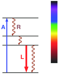
Figure 1: (Color online) Sketch of the processes relevant for optical spectroscopies. A: absorption; L: luminescence; R: radiationless transition.

A variant of the absorption and luminescence spectroscopies, associated with initial transitions to discrete excited energy states, is the Raman spectroscopy Larkin (2011) where the system is excited to a virtual energy state and then quickly relaxes back to a ground-state level. Unlike a luminescence process, Raman scattering involves no transfer of electron population to the intermediate state. Several variations of Raman spectroscopy have been developed in order to enhance the sensitivity [e.g., surface-enhanced Raman spectroscopy Lombardi and Birke (2008) and resonance Raman spectroscopy Chao et al. (1976)] as well as to improve the spatial resolution [Raman microscopy Turrell and Corset (1996)].

Optical spectroscopies are governed by the energy and momentum conservation laws as in neutron spectroscopy, see Eqs. (14) and (15). However, as the photon wave vector is about 10³ times smaller than a typical reciprocal lattice vector, only excitations close to the center of the Brillouin zone are observed. The calculation of intensities of the observed transitions is a non-trivial task. This is in contrast to neutron spectroscopy where the intensities of spin excitations are directly proportional to the square of the magnetic dipole matrix elements, Eq. (18). Since optical spectroscopies often involve intermediate states which are not known, approximate models have to be employed for the calculation of transition matrix elements Lovesey and Collins (1996).

The polarization of light has great importance particularly when anisotropic systems are studied. The specific polarization of both the exciting and the emitted light can be exploited to obtain extra information concerning the line identification from the observed energy spectra. More specifically, electronic states with transition dipole moments perpendicular to the electric field orientation will not be excited.

II.2.3 Electron Paramagnetic Resonance

In EPR spectroscopy the absorption of a radio-frequency (rf) magnetic field ${\bf B}^{rf}$ by a magnetic system is measured Abragam and Bleaney (1986). Absorption can occur whenever the energy $h\nu$ of the radiation matches the energy difference of two eigen states $|\lambda\rangle$ and $|\lambda^{\prime}\rangle$,

$$E_{\lambda^{\prime}}-E_{\lambda}=\pm h\nu,$$ (35)

and the absorbed power $P$ is calculated in linear response theory to

$$P = C(\omega)\sum_{\alpha\beta}B_{\alpha}^{rf}B_{\beta}^{rf}\sum_{ij}\sum_{\lambda\lambda^{\prime}}p_{\lambda}\langle\lambda|\hat{s}_{i\alpha}|\lambda^{\prime}\rangle\langle\lambda^{\prime}|\hat{s}_{j\beta}|\lambda\rangle$$ (36)

$$\times\delta(\hbar\omega+E_{\lambda}-E_{\lambda^{\prime}}),$$

with $C(\omega)=\omega[1-\exp(\hbar\omega/k_{B}T)](g^{2}\mu_{B}^{2})/(8\hbar\pi)$. For magnetic cluster systems with eigen states $|\tau SM\rangle$, Eq. (36) can be further evaluated and the EPR selection rules

$$\Delta S=0,$$ (37)

$$\Delta M=\pm 1,$$ (38)

established from $\sum_{i}\langle\lambda|\hat{s}_{i\alpha}|\lambda^{\prime}\rangle=\langle\tau SM|\hat{S}_{\alpha}|\tau^{\prime}S^{\prime}M^{\prime}\rangle$.

It follows that EPR spectroscopy is a very direct method to determine anisotropies of the $g$ factor by aligning the external magnetic field ${\bf B}$ along different directions. Similarly, anisotropies of the form defined by, e.g., Eqs. (10) and (11), which lift the degeneracy of a particular spin multiplet, can also be determined from the positions of the lines in the EPR spectra. On the other hand, the exchange splittings or parameters $J_{ij}$ are not directly attainable, but they can be estimated from the temperature variation of the signal intensities which follow the Boltzmann populations of the energy levels involved, or in some fortunate cases through the $S$-mixing mechanism Wilson et al. (2006). Finally we point to the distinctive hyperfine structure superimposed on an EPR spectrum for systems with non-zero nuclear spin quantum numbers.

It is instructive to compare Eq. (36) to the corresponding INS formula Eq. (16) with Eq. (18). The main difference lies in the structure factor $\exp({\bf Q}\cdot{\bf R}_{ij})$ which is 1 in case of EPR corresponding to ${\bf Q}=0$ in INS. Therefore, EPR affords the detection of exactly those magnetic transitions which have INS intensity at ${\bf Q}\rightarrow 0$, which in the HDVV model are the $\Delta S=0$ transitions. Physically speaking, in contrast to a neutron the applied radio frequency establishes a frequency-dependent but spatially homogeneous magnetic field, ${\bf B}({\bf Q},\omega)$ with ${\bf Q}=0$.

Modern EPR spectroscopy techniques permit a large combination of frequency and magnetic field values extending up to the THz regime and 25 T, respectively. In principle, EPR spectra can be generated by either varying the frequency $\nu$ while holding the magnetic field constant, or doing the reverse. In commercial EPR instruments it is the frequency which is kept fixed, and typical frequencies are X-band (10 GHz) and Q-band (35 GHz), but W-band (95 GHz) is also available. However, the EPR techniques have progressed enormously, and multi-frequency high-field EPR and frequency domain magnetic resonance spectroscopy (FDMRS) experiments are routinely undertaken in various laboratories. A recent development are THz EPR experiments using radiation from synchrotron sources. For reviews see Gatteschi et al. (2006a); van Slageren et al. (2003).

II.2.4 Thermodynamic Magnetic Properties

The thermodynamic magnetic properties depend explicitly upon both the energies $E_{\lambda}$ and the eigen functions $|\lambda\rangle$ of the spin excitations. Based on general expressions of statistical mechanics for the Gibbs free energy $F$ and internal energy $U$,

$$F = -k_{B}T\ln Z,$$ (39)

$$U = F-T\left(\frac{\partial F}{\partial T}\right)_{V},$$ (40)

we obtain, with the Zeeman term as in Eq. (13), the magnetization $M_{\alpha}$, magnetic susceptibility $\chi_{\alpha\alpha}$, entropy $S$, and Schottky heat capacity $c_{V}$:

$$M_{\alpha} = -\frac{\partial F}{\partial B_{\alpha}}=-g\mu_{B}\sum_{\lambda}p_{\lambda}\langle\lambda|\hat{S}_{\alpha}|\lambda\rangle,$$ (41)

$$\chi_{\alpha\alpha} = \frac{\partial M_{\alpha}}{\partial B_{\alpha}}=\frac{\left(g\mu_{B}\right)^{2}}{k_{B}T}$$

$$\times\left[\sum_{\lambda}p_{\lambda}\langle\lambda|\hat{S}_{\alpha}^{2}|\lambda\rangle-\left(\sum_{\lambda}p_{\lambda}\langle\lambda|\hat{S}_{\alpha}|\lambda\rangle\right)^{2}\right],$$

$$S = -\left(\frac{\partial F}{\partial T}\right)_{V}=k_{B}\left(\ln Z+\frac{\sum_{\lambda}p_{\lambda}E_{\lambda}}{k_{B}T}\right),$$ (43)

$$c_{V} = \left(\frac{\partial U}{\partial T}\right)_{V}$$ (44)

$$= \frac{1}{k_{B}T^{2}}\left[\sum_{\lambda}p_{\lambda}E^{2}_{\lambda}-\left(\sum_{\lambda}p_{\lambda}E_{\lambda}\right)^{2}\right].$$

Here, $Z$ and $p_{\lambda}$ are the partition function and Boltzmann population factor, respectively:

$$Z=\sum_{\lambda}\exp(-\frac{E_{\lambda}}{k_{B}T}),\quad p_{\lambda}=\frac{1}{Z}\exp(-\frac{E_{\lambda}}{k_{B}T}).$$ (45)

For a system with magnetic anisotropy also the magnetic torque $\bf\tau$ appears as a useful thermodynamic quantity:

$$\tau=\frac{\partial F}{\partial\theta},\quad{\bf\tau}={\bf M}\times{\bf B},$$ (46)

where $\theta$ denotes the rotation angle around the torque axis [often the definition $\tau=-\partial F/\partial\phi$ is found, our convention is consistent with the usual parametrization of magnetic field, e.g., ${\bf B}=B(\sin\theta,0,\cos\theta)$].

For $T\rightarrow 0$, the free energy reduces to the ground-state energy $E_{0}$ and the magnetization to the field derivative $M_{\alpha}=-\partial E_{0}/\partial B_{\alpha}$. As function of field the ground state often undergoes level crossings at characteristic fields, which can be detected at very low temperatures as steps in the field-dependent magnetization (torque) curves. The characteristic fields allow insight into the magnetic excitation spectrum in a cluster, and low-temperature high-field magnetization (torque) measurements represent an important experimental technique Shapira and Bindilatti (2002), though the level crossing can also be detected by other techniques, e.g., proton nuclear magnetic resonance Julien et al. (1999). In order to check the reliability of the model parameters derived from spectroscopic data, it is however generally useful to compare the calculated thermodynamic magnetic properties to corresponding experimental data.

III Small magnetic clusters

The aim of this section is to demonstrate how the various interactions introduced in Sec. II.1 manifest themselves for different experimental techniques. The presented examples will be restricted to small clusters built up by $N\leq 4$ coupled magnetic ions, for which the underlying models can be treated exactly, since only a small number of interactions are present and cooperative effects do not occur, so that a straightforward comparison between theory and experiment is possible with little ambiguity. The examples cover magnetic clusters which naturally occur in pure compounds as well as clusters which are artificially formed in solid solutions of magnetic and nonmagnetic compounds. Ideal examples of pure compounds are molecular transition-metal complexes, in which a polynuclear metal core is embedded in a diamagnetic ligand matrix. Information more directly associated with cooperative systems results from diluted magnetic compounds, in which the magnetic ions are randomly distributed, so that different types of clusters ($N$-mers, $N=1,2,3,...$) are simultaneously present. Among the myriads of small magnetic cluster systems studied up to the present we will choose as a representative of the pure compounds the dimeric chromium system [(NH₃)₅CrOHCr(NH₃)₅]Cl₅$\cdot$H₂O, which is the first magnetic cluster system investigated by INS. The class of magnetically diluted systems was pioneered in INS experiments carried out for the compound KMn_xZn_1-xF₃ Svensson et al. (1978) and will be exemplified here by the compound CsMn_xMg_1-xBr₃. The chapter ends with further insights on particular physical aspects resulting from magnetic cluster excitations on some other compounds.

III.1 The dimeric chromium compound [(NH₃)₅CrOHCr(NH₃)₅]Cl₅$\cdot$H₂O

III.1.1 Energy levels

The simplest magnetic cluster system is the dimer (two coupled spins $\hat{\bf s}_{1}$ and $\hat{\bf s}_{2}$) for which the HDVV Hamiltonian Eq. (2) simplifies to

$$\hat{H}=-2J\hat{\bf{s}}_{1}\cdot\hat{\bf{s}}_{2}.$$ (47)

Assuming identical magnetic ions ($s_{1}=s_{2}=s$) the eigenvalues of Eq. (47) are

$$E(S)=-J\left[S(S+1)-2s(s+1)\right],$$ (48)

with $0\leq S\leq 2s$. The energy splittings defined by Eq. (48) satisfy the Landé interval rule

$$E(S)-E(S-1)=-2JS.$$ (49)

For Cr³⁺ dimers with $s=3/2$ the separation between the ground-state levels will be $2J$, $4J$, and $6J$ ($S=0$ to $S=3$), with the state $S=0$ being the lowest in case of AFM exchange $J<0$. Observed deviations from the Landé interval rule are often attributed to the presence of biquadratic exchange,

$$\hat{H}=-K\left(\hat{\bf{s}}_{1}\cdot\hat{\bf{s}}_{2}\right)^{2}.$$ (50)

Combining Eqs. (47) and (50) yields the modified eigenvalues

$$E(S) = -J\eta-\frac{1}{4}K\eta^{2},$$ (51)

$$\eta = S(S+1)-2s(s+1).$$ (52)

III.1.2 Structural and magnetic characterization

The compound [(NH₃)₅CrOHCr(NH₃)₅]Cl₅$\cdot$H₂O was characterized by X-ray diffraction, EPR, and magnetic susceptibility measurements Veal et al. (1973). The material crystallizes in the tetragonal space group P4₂/mnm with four formula units in a cell of dimensions $a=16.259(7)$ Å and $c=7.411(7)$ Å. The two Cr³⁺ ions are coupled by superexchange via a Cr-O-Cr bridge with a bridging angle of 165.6(9)^∘ and a Cr-O distance of 1.94(1) Å. The analysis of the X-ray data requires two inequivalent positions of Cr³⁺ dimers in the unit cell. EPR measurements gave a negligibly small upper limit of $D\leq 0.002$ meV for the single-ion anisotropy defined by Eq. (10). The magnetic susceptiblity was measured for a polycrystalline sample as shown in Fig. 2. The data were analyzed according to Eq. (II.2.4) with $g=1.99$ resulting from the EPR experiments. The agreement between the observed and calculated data is slightly improved when in addition to the Heisenberg exchange Eq. (47) a biquadratic term Eq. (50) is included.

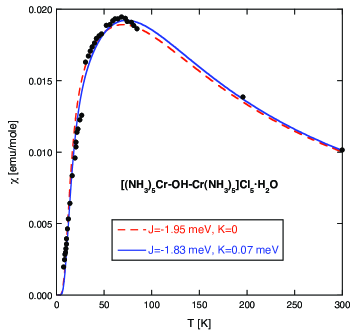
Figure 2: (Color online) Temperature dependence of the magnetic susceptibilty of [(NH₃)₅CrOHCr(NH₃)₅]Cl₅$\cdot$H₂O. Adapted from Veal et al., 1973.

III.1.3 Optical spectroscopies

Optical spectroscopies were applied to single crystals of [(NH₃)₅CrOHCr(NH₃)₅]Cl₅$\cdot$H₂O Ferguson and Güdel (1973). Both polarized absorption and polarized luminescence spectra provided well resolved lines from which the ground-state level scheme could be directly determined. Figure 3 shows a representative polarized luminescence spectrum with two sets of transitions (A’,B’,C’) and (A”,B”,C”) reflecting the presence of two inequivalent dimer sites. The emission starts from an excited state with $S=2$. The appearance of three lines for each of the transitions indicates that the selection rule $\Delta S=0$ is not exact, but transitions also occur for $\Delta S=\pm 1$ (with much smaller intensities) due to the spin-orbit interaction. The luminescence spectrum accurately determines the separations between the ground-state levels $S=1,2,$ and 3, and the separation between $S=0$ and $S=1$ was taken from the absorption spectrum. The ground-state level scheme slightly deviates from the Landé interval rule, so that the data analysis was based on Eq. (51). The resulting bilinear and biquadratic exchange parameters $J$ and $K$ are listed in Table 1. The luminescence spectrum is strongly temperature dependent, and it is completely quenched at room temperature.

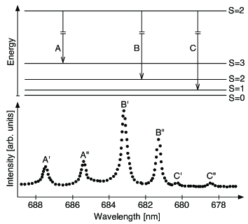
Figure 3: Polarized luminescence spectrum of [(NH₃)₅CrOHCr(NH₃)₅]-Cl₅$\cdot$H₂O taken at $T=7$ K. The corresponding transition diagram is shown at the top. Adapted from Ferguson and Güdel, 1973.

III.1.4 Inelastic neutron scattering

For the analysis of the neutron data we adjust the magnetic scattering function Eq. (18) to the dimer case. We start from the reduced matrix elements introduced in Eq. (II.2.1). Since $\hat{T}^{1}(s_{i})$ operates only on the $i$th ion of the coupled system, the reduced matrix elements can be further simplified:

$$\langle S||\hat{T}^{1}(s_{1})||S^{\prime}\rangle = (-1)^{2s+S+1}\sqrt{(2S+1)(2S^{\prime}+1)}$$ (55)

$$\times\left\{\begin{array}[]{ccc}S&S^{\prime}&1\\ s&s&s\end{array}\right\}\langle s|||\hat{T}^{1}(s)|||s\rangle,$$

$$\langle S||\hat{T}^{1}(s_{2})||S^{\prime}\rangle = (-1)^{S^{\prime}-S}\langle S||\hat{T}^{1}(s_{1})||S^{\prime}\rangle,$$ (56)

$$\langle s|||\hat{T}^{1}(s)|||s\rangle = \sqrt{s(s+1)(2s+1)}.$$ (57)

The two-row bracket $\{...\}$ in Eq. (55) is a Wigner-$6j$ symbol Rotenberg et al. (1959) which vanishes unless $\Delta S=0,\pm 1$. From Eqs. (23) and (55) the INS selection rules $\Delta M=0,\pm 1$ and $\Delta S=0,\pm 1$ are recovered. By making use of the symmetry properties of the reduced matrix elements defined by Eq. (55), we find the following cross section for the dimer transition $|S\rangle\rightarrow|S^{\prime}\rangle$:

$$\frac{d^{2}\sigma}{d\Omega d\omega} = C({\bf Q})\frac{\exp[-\frac{E(S)}{k_{B}T}]}{Z}\sum_{\alpha}\left[1-\left(\frac{Q_{\alpha}}{Q}\right)^{2}\right]$$ (58)

$$\times\frac{2}{3}\left[1+(-1)^{\Delta S}\cos({\bf Q}\cdot{\bf R})\right]\langle S||\hat{T}^{1}(s_{1})||S^{\prime}\rangle^{2}$$

$$\times\delta[\hbar\omega+E(S)-E(S^{\prime})],$$

where ${\bf R}={\bf R}_{1}-{\bf R}_{2}$ is the vector defining the intra-dimer separation. The structure factor $[1+(-1)^{\Delta S}\cos({\bf Q}\cdot{\bf R})]$ is a powerful means to unambiguously identify dimer excitations from other scattering contributions due to its characteristic oscillating behavior.

For a polycrystalline material Eq. (58) has to be averaged in $\bf Q$ space:

$$\frac{d^{2}\sigma}{d\Omega d\omega} = C(Q)\frac{\exp[-\frac{E(S)}{k_{B}T}]}{Z}\frac{4}{3}\left[1+(-1)^{\Delta S}\frac{\sin(QR)}{QR}\right]$$

$$\times\langle S||\hat{T}^{1}(s_{1})||S^{\prime}\rangle^{2}\delta[\hbar\omega+E(S)-E(S^{\prime})].$$

The polarization and structure factors combine to the interference factor $[1+(-1)^{\Delta S}\sin(QR)/(QR)]$, which produces a damped oscillatory $Q$ dependence of the intensities.

Figure 4(a) shows the temperature dependence of neutrons scattered from a polycrystalline sample of deuterated [(NH₃)₅CrOHCr(NH₃)₅]Cl₅$\cdot$H₂O Furrer and Güdel (1977); Güdel et al. (1981), which demonstrates the successive appearance of the excited-state transitions with increasing temperature. The data confirm the ground-state splitting pattern sketched on top of Fig. 3. The resulting parameters based on Eq. (51) are listed in Table 1. The oscillatory behavior of the intensities vs the modulus of the scattering vector $\bf Q$ predicted by Eq. (III.1.4) is nicely verified as shown in Fig. 4(b).

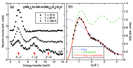
Figure 4: (Color online) (a) Energy spectra of neutrons scattered from deuterated [(NH₃)₅CrOHCr(NH₃)₅]Cl₅$\cdot$H₂O. (b) $Q$ dependence of the intensity of the $|0\rangle\rightarrow|1\rangle$ transition observed at $T=4.2$ K shown in panel (a). Adapted from (a) Güdel et al., 1981 and (b) Furrer and Güdel, 1977.

III.1.5 Comparison of different experimental techniques

Table 1 lists the results obtained by different experimental techniques presented in the preceding subsections. From the EPR measurements the anisotropic magnetic effects associated with the compound [(NH₃)₅CrOHCr(NH₃)₅]Cl₅$\cdot$H₂O were established to be negligibly small. This was verified in subsequent light and neutron spectroscopic investigations, which did not give evidence for any anisotropy-induced line splittings. Due to the excellent energy resolution, light spectroscopies provide at low temperatures rather precise spin coupling parameters, but information on their temperature dependence is severely hampered because of signal quenching. This is not the case for inelastic neutron scattering, which gives evidence for a strong temperature dependence of the bilinear exchange parameter $J$ of the order of 15% upon heating from 7 K to room temperature. The analysis of the magnetic susceptibility data thus results in a temperature-averaged parameter $J$, and it overestimates the biquadratic coupling parameter $K$ by a factor of 2.

Table 1: Coupling parameters $J$ and $K$ of [(NH₃)₅CrOHCr(NH₃)₅]Cl₅$\cdot$H₂O determined by different experimental techniques.

Technique	$T$ [K]	$J$ [meV]	$K$ [meV]
mag. suscept.	7-300	-1.83	0.07
light spec.	7	-1.91(1)	0.02(1)
INS	30	-1.88(5)	0.03(2)
INS	165	-1.83(8)	0.02(4)
INS	293	-1.74(14)	0.03(7)

III.2 Manganese $N$-mers in CsMn_xMg_1-xBr₃

III.2.1 Structural and magnetic characterization

Solid solutions of composition CsMn_xMg_1-xBr₃ are ideal model systems for various reasons. Both CsMnBr₃ and CsMgBr₃ crystallize in the hexagonal space group P6₃/mmc, and their unit cell parameters are almost equal: $a=b=7.609(15)$ Å, $c=6.52(5)$ Å for CsMnBr₃ Goodyear and Kennedy (1972) and $a=b=7.610(2)$ Å, $c=6.502(2)$ Å for CsMgBr₃ McPherson et al. (1980). The structure consists of chains of face-sharing MBr₆ octahedra parallel to the $c$ axis, where M is Mn²⁺ ($s=5/2$) or Mg²⁺ (diamagnetic). Spin-wave experiments gave evidence for a pronounced one-dimensional magnetic behavior with the intra-chain exchange interaction exceeding the inter-chain exchange interaction by three orders of magnitude Breitling et al. (1977); Falk et al. (1987b). All the Mn²⁺ clusters in the mixed compound CsMn_xMg_1-xBr₃ are thus linear chain fragments with composition Mn_NBr_3(N+1) ($N=1,2,3,...$) oriented parallel to the $c$ axis. The Mn²⁺ clusters are statistically distributed with the probability $p_{N}(x)$ for $N$-mer formation given by

$$p_{N}(x)=(1-x)x^{N-1}.$$ (60)

For Mn²⁺ concentrations $x<0.05$, monomers and dimers dominate, but for $x>0.05$ trimers, tetramers, etc. have to be considered. For the ground-state splitting pattern of dimers we refer to Sec. III.1.1. The energy levels of linear trimers and tetramers are summarized below.

III.2.2 Energy levels of linear trimers and tetramers

The HDVV Hamiltonian of a linear trimer is defined by

$$\hat{H}=-2J\left(\hat{\bf{s}}_{1}\cdot\hat{\bf{s}}_{2}+\hat{\bf{s}}_{2}\cdot\hat{\bf{s}}_{3}\right)-2J^{\prime}\hat{\bf{s}}_{1}\cdot\hat{\bf{s}}_{3}.$$ (61)

It is convenient to introduce the spin quantum numbers $S_{13}$ and $S$ resulting from the spin coupling scheme defined by the vector sums $\hat{\bf S}_{13}=\hat{\bf s}_{1}+\hat{\bf s}_{3}$ and $\hat{\bf S}=\hat{\bf s}_{2}+\hat{\bf S}_{13}$ with $0\leq S_{13}\leq 2s$ and $|S_{13}-s|\leq S\leq(S_{13}+s)$, respectively, assuming $s_{1}=s_{2}=s_{3}=s$. The trimer states are therefore defined by $|S_{13}SM\rangle$, and their degeneracy is $(2S+1)$. With this choice of spin quantum numbers, the Hamiltonian Eq. (61) is diagonal and the eigenvalues can thus readily be derived as

$$E(S_{13},S) = -J\left[S(S+1)-S_{13}(S_{13}+1)-s(s+1)\right]$$ (62)

$$-J^{\prime}\left[S_{13}(S_{13}+1)-2s(s+1)\right].$$

The HDVV Hamiltonian of a linear tetramer is given by

$$\hat{H} = -2J\left(\hat{\bf{s}}_{1}\cdot\hat{\bf{s}}_{2}+\hat{\bf{s}}_{2}\cdot\hat{\bf{s}}_{3}+\hat{\bf{s}}_{3}\cdot\hat{\bf{s}}_{4}\right)$$ (63)

$$-2J^{\prime}\left(\hat{\bf{s}}_{1}\cdot\hat{\bf{s}}_{3}+\hat{\bf{s}}_{2}\cdot\hat{\bf{s}}_{4}\right)-2J^{\prime\prime}\hat{\bf{s}}_{1}\cdot\hat{\bf{s}}_{4}.$$

To solve Eq. (63), the total spin $\hat{\bf S}=\hat{\bf s}_{1}+\hat{\bf s}_{2}+\hat{\bf s}_{3}+\hat{\bf s}_{4}$ is still a good quantum number, but for a complete characterization of the tetramer states additional intermediate spin quantum numbers are needed, e.g., $\hat{\bf S}_{12}=\hat{\bf s}_{1}+\hat{\bf s}_{2}$ and $\hat{\bf S}_{34}=\hat{\bf s}_{3}+\hat{\bf s}_{4}$ with $0\leq S_{12}\leq 2s$ and $0\leq S_{34}\leq 2s$, respectively. The total spin is then defined by $|S_{12}-S_{34}|\leq S\leq(S_{12}+S_{34})$, and the basis states are the wave functions $|S_{12}S_{34}SM\rangle$. There is no spin coupling scheme which results in a diagonal Hamiltonian matrix, so that the eigenvalues of Eq. (63) have to be calculated numerically or by spin-operator techniques Judd (1963).

III.2.3 Electron paramagnetic resonance

Single crystals of CsMgBr₃ doped with Mn²⁺ ions ($s=5/2$) were studied by EPR measurements at Q- and X-band frequencies with the magnetic field parallel and perpendicular to the $c$ axis McPherson et al. (1974). The EPR spectrum displayed in Fig. 5 shows the hyperfine and fine structures expected for Mn²⁺ ions in an axial environment. The Q-band frequency of $\nu=35$ GHz produces five resonances A to E whenever the spacing of adjacent Zeeman-split energy levels corresponds to $\Delta E=0.145$ meV [see Eq. (35)] as illustrated in Fig. 6. Each resonance is characterized by six oscillations due to the hyperfine interaction, since the nuclear spin of manganese is $I=5/2$. The positions of the five resonances do not occur at equidistant spacings, which indicates the presence of a non-zero single-ion anisotropy. From the positions of the resonances the Landé splitting factor $g=2.004(1)$ and the axial anisotropy parameter $|D|=0.0115(2)$ meV were obtained. Note that the sign of $D$ cannot be determined from EPR experiments at elevated temperatures.

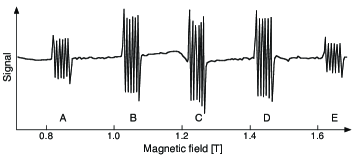
Figure 5: Q-band EPR spectrum of Mn²⁺ ions in CsMgBr₃ at $T=77$ K. Adapted from McPherson et al., 1974.

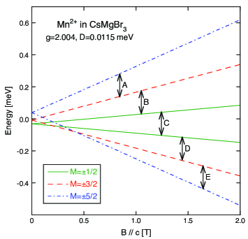
Figure 6: (Color online) Field dependence of the ground-state levels of Mn²⁺ ions in CsMgBr₃. The calculations are based on Eqs. (10) and (13), with $D>0$. The double arrows mark the resonances A to E observed in the EPR spectrum of Fig. 5.

III.2.4 Optical spectroscopies

Single crystals of CsMn_xMg_1-xBr₃ ($0.04\leq x\leq 0.20$) were investigated by optical spectroscopies McCarthy and Güdel (1984). In particular, Mn²⁺ pair excitations were observed in the absorption spectra as shown in Fig. 7. The weak absorptions at $T=1.4$ K cannot be assigned with certainty; they are either single-ion absorptions or due to Mn²⁺ clusters with $N>3$. With increasing temperature additional bands appear due to the successive population of the cluster states $S=1$ to $S=4$. The temperature dependence of the intensities is best described by using the HDVV Hamiltonian Eq. (48) with $J=-0.88$ meV as illustrated in Fig. 7.

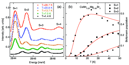
Figure 7: (Color online) (a) Temperature dependence of absorption spectra resulting from a spin-flip process observed for CsMn_0.20Mg_0.80Br₃. The successive population of the Mn²⁺ dimer states is marked by $S=1$ to $S=4$. (b) Observed intensities of the bands $S=1$ to $S=3$ as a function of temperature. The lines correspond to the Boltzmann populations calculated from Eq. (48) with $J=-0.88$ meV . Adapted from McCarthy and Güdel, 1984.

III.2.5 Inelastic Neutron Scattering

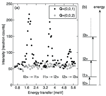
Figure 8: (a) Energy spectra of neutrons scattered from Mn²⁺ pairs in CsMn_0.28Mg_0.72Br₃ at $T=30$ K. (b) Energy-level sequence of an antiferromagnetically coupled spin pair. Adapted from Falk et al., 1984.

INS experiments performed on a single crystal of CsMn_0.28Mg_0.72Br₃ gave evidence for well defined Mn²⁺ dimer transitions as shown in Fig. 8 Falk et al. (1984). The observed intensities are in excellent agreement with the predictions by the structure factor Eq. (58); with ${\bf R}=(0,0,1/2)$ the intensity has a maximum for ${\bf Q}=(0,0,1)$ and vanishes for ${\bf Q}=(0,0,2)$. The energies of the transitions $|0\rangle\rightarrow|1\rangle$, $|1\rangle\rightarrow|2\rangle$, $|2\rangle\rightarrow|3\rangle$, and $|3\rangle\rightarrow|4\rangle$ turned out to be 1.80(1), 3.60(1), 5.27(2), and 6.74(3) meV, which considerably deviate from the Landé interval rule, so that the data analysis was based on Eq. (51). The resulting parameters are $J=-838(5)$ $\mu$eV and $K=8.8(8)$ $\mu$eV.

Table 2: Resulting parameters from least-squares fits to the observed Mn trimer transitions in CsMn_0.28Mg_0.72Br₃ Falk et al. (1986).

Model	$J$ [$\mu$eV]	$J^{\prime}$ [$\mu$eV]	$K$ [$\mu$eV]	$L$ [$\mu$eV]	$\chi^{2}$
a $(K=L=0)$	-870(12)	-8(14)	0	0	5.22
b $(K\neq 0,L=0)$	-786(7)	-12(10)	14(2)	0	3.13
c $(K\neq 0,L\neq 0)$	-777(6)	-11(9)	8(1)	6(1)	1.67

Later INS experiments gave evidence for well defined Mn³⁺ trimer and tetramer transitions Falk et al. (1987a). For the evaluation of the differential neutron cross section we refer to references in Sec. II.2.1. For a trimer the selection rules of the transition $|S_{13}SM\rangle\rightarrow|S_{13}^{\prime}S^{\prime}M^{\prime}\rangle$ are derived as

$$\Delta S = 0,\pm 1,$$ (64)

$$\Delta S_{13} = 0,\pm 1,$$ (65)

$$\Delta M = 0,\pm 1.$$ (66)

The smallest magnetic systems to identify three-spin interactions are spin trimers. The bilinear Hamiltonian Eq. (61) has to be extended in the following way:

$$\hat{H} = -2J\left(\hat{\bf{s}}_{1}\cdot\hat{\bf{s}}_{2}+\hat{\bf{s}}_{2}\cdot\hat{\bf{s}}_{3}\right)-2J^{\prime}\hat{\bf{s}}_{1}\cdot\hat{\bf{s}}_{3}$$ (67)

$$-K\left[\left(\hat{\bf{s}}_{1}\cdot\hat{\bf{s}}_{2}\right)^{2}+\left(\hat{\bf{s}}_{2}\cdot\hat{\bf{s}}_{3}\right)^{2}\right]-K^{\prime}\left(\hat{\bf{s}}_{1}\cdot\hat{\bf{s}}_{3}\right)^{2}$$

$$-L\left[\left(\hat{\bf{s}}_{1}\cdot\hat{\bf{s}}_{2}\right)\left(\hat{\bf{s}}_{2}\cdot\hat{\bf{s}}_{3}\right)+\left(\hat{\bf{s}}_{3}\cdot\hat{\bf{s}}_{2}\right)\left(\hat{\bf{s}}_{2}\cdot\hat{\bf{s}}_{1}\right)\right].$$

$K$, $K^{\prime}$, and $L$ denote biquadratic two-spin and three-spin exchange parameters, respectively, which give rise to off-diagonal matrix elements, so that Eq. (67) was diagonalized in first-order perturbation theory. The biquadratic $K^{\prime}$ term is neglected, since $|K^{\prime}|\ll|K|$. The low-energy part of the eigenvalues $E(S_{13},S)$ is illustrated in Fig. 9 for the case of Mn trimer excitations in CsMn_0.28Mg_0.72Br₃, which were identified in INS experiments according to the characteristic dependence of the cross section Eq. (16) upon $\bf Q$ and $T$ Falk et al. (1986). The observed transitions are marked by arrows in Fig. 9. Least-squares fits based on Eq. (67) with different parameter selection gave the results listed in Table 2. The model including only bilinear exchange interactions failed as expected. The model including the bilinear and biquadratic terms of the Hamiltonian Eq. (67) resulted in an improved standard deviation $\chi^{2}$, but only the least-squares fit including the three-spin interaction was able to reproduce the observed transitions satisfactorily.

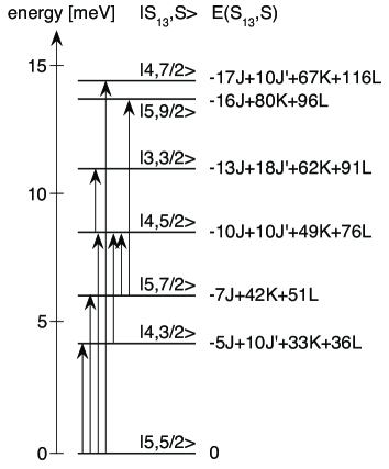
Figure 9: Energy level splittings of Mn trimers in CsMn_0.28Mg_0.72Br₃. The arrows denote the observed transitions. Adapted from Falk et al., 1986.

Recent INS experiments performed with increased instrumental energy resolution gave evidence for anisotropy-induced splittings of Mn²⁺ dimer and tetramer transitions Furrer et al. (2011a). This is demonstrated in Fig. 10 for the dimer $|S=0\rangle\rightarrow|S=1\rangle$ transition. There are two well defined lines A and B which according to the approximate intensity ratio 2:1 can be attributed to the $|S=0,M=0\rangle\rightarrow|S=1,M=\pm 1\rangle$ and $|S=0,M=0\rangle\rightarrow|S=1,M=0\rangle$ transitions, respectively. A similar anisotropy-induced splitting was observed for the lowest tetramer $|S=0\rangle\rightarrow|S=1\rangle$ transition as well. The dimer and tetramer data could be rationalized by the combined action of a single-ion anisotropy parameter $D=0.0183(16)$ meV defined by Eq. (10) and of two-ion anisotropic coupling parameters $J=J_{xx}=J_{yy}=-0.852(3)$ meV and $J_{zz}/J=0.997(1)$ defined by Eq. (3). The two-ion anisotropy is most likely due to the anisotropic part of the dipole-dipole interaction Eq. (4). The exchange coupling $J$ is sufficiently strong to keep the spins $\hat{\bf s}_{i}$ antiferromagnetically aligned at low temperatures $T\leq|J|/k_{B}$, but their direction with respect to ${\bf R}||{\bf c}$ is free to rotate. Therefore, the second term of Eq. (4) has to be averaged in space:

$$\hat{H}=\sum_{ij}\frac{g^{2}\mu_{B}^{2}}{R^{3}_{ij}}\left[\hat{\bf{s}}_{i}\cdot\hat{\bf{s}}_{j}-3\frac{(\hat{\bf{s}}_{i}\cdot{\bf{R}}_{ij})(\hat{\bf{s}}_{j}\cdot{\bf{R}}_{ij})}{\pi^{2}R^{2}_{ij}}\right],$$ (68)

The dipole-dipole anisotropy calculated from Eq. (68) is $J_{zz}/J=0.997$, in agreement with the experimental findings.

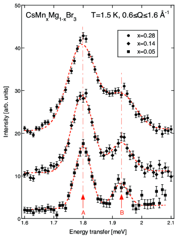
Figure 10: (Color online) Energy spectra of neutrons scattered from CsMn_xMg_1-xBr₃. The energy resolution amounts to 55 $\mu$eV. For clarity, the data for $x=0.14$ and 0.28 are shifted by 10 and 20 intensity units, respectively. The lines refer to Gaussian peak fits with equal line widths for both transitions A and B. Adapted from Furrer et al., 2011a.

III.2.6 Comparison of different experimental techniques

Table 3 lists the results obtained by different experimental techniques presented in the preceding subsections. The sign of the axial anisotropy parameter $D$ could unambiguously be determined by neutron spectroscopy, in contrast to the EPR experiments. The parameters $D$ and $J$ exhibit a pronounced temperature dependence probably due to the lattice expansion with increasing $T$, whereas the parameter $K$ remains constant. Since the analysis of the optical data was based on a model with $K=0$, the resulting exchange parameter $J$ cannot be compared with the results of the INS experiments. It was shown in Falk et al., 1984; Strässle et al., 2004 that the presence of biquadratic exchange ($K\neq 0$) is caused to a major extent by the mechanism of exchange striction Kittel (1960).

Table 3: Axial anisotropy parameter $D$ and spin coupling parameters $J$ and $K$ of Mn²⁺ dimers in CsMn_xMg_1-xBr₃ determined by different experimental techniques.

Technique	$T$ [K]	$D$ [meV]	$J$ [meV]	$K$ [meV]
EPR	77	$\pm$0.0115(2)	-	-
Optical	13	-	-0.88	-
INS	30	-	-0.838(5)	0.0088(8)
INS	50	-	-0.823(1)	0.0087(2)
INS	1.5	0.0183(16)	-0.852(3)	0.0086(2)

In extended antiferromagnets the observation of the spin-wave dispersion by single-crystal INS experiments is usually the most common approach to determine exchange parameters. By applying the spin-wave formalism to $\hat{H}$ from Eq. (67), which includes higher-order exchange terms, we find

$$\hbar\omega(q) = 4s|J_{eff}|\sin(qc),$$ (69)

$$J_{eff} = -|\sqrt{J(J-4J^{\prime})}+\frac{5s}{2}(K+2L)|,$$ (70)

where $q$ is the wave number of the spin wave propagating along the $c$ axis. From spin-wave experiments performed for the one-dimensional antiferromagnet CsMnBr₃ ($s=5/2$) the exchange coupling was determined to be $J_{eff}=-0.89(2)$ meV Breitling et al. (1977); Falk et al. (1987b). The analysis of the spin-wave dispersion just yields an effective exchange parameter $J_{eff}$, but the individual sizes of the bilinear and biquadratic exchange parameters cannot be determined. This is in contrast to experiments on small magnetic clusters as discussed in the preceding sections. A numerical comparison of the $J_{eff}$ values obtained from the three models listed in Table 2 is interesting. Using Eq. (67) and $s=5/2$ we find $J_{eff}=-0.89(2)$, -0.90(3) and -0.92(3) meV for models a, b and c, respectively. The three values are identical within experimental error, and they excellently agree with $J_{eff}$ determined from spin-wave experiments. They also agree with $J_{eff}=-0.88$ meV derived from the optical spectroscopies applied to the Mn²⁺ dimer excitations, see Table 3. $J_{eff}$ is obviously independent of the geometric size of the coupled magnetic ions and can therefore be regarded as a measure of the magnetic energy per Mn²⁺ ion in the AFM state of CsMnBr₃.

III.3 Further insights from magnetic cluster excitations

III.3.1 Exchange parameters from high-field magnetization steps

Step-like features in high-field magnetization data result from level crossings associated with the ground state of magnetic clusters and thereby provide information about the exchange parameters. This is demonstrated here for the tetrameric nickel compound [Mo₁₂O₂₈(OH)₁₂{Ni(H₂O)₃}₄]$\cdot$13H₂O, henceforth abbreviated as {Ni₄Mo₁₂}. The magnetization is enhanced from zero up to the saturation value of 8 $\mu_{B}$ in steps of 2 $\mu_{B}$ at the fields 4.5, 8.9, 20.1, and 32 T as illustrated by the differential magnetization data in Fig. 11 Schnack et al. (2006).

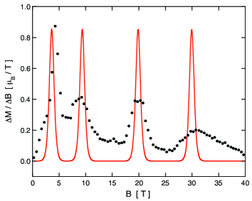
Figure 11: (Color online) High-field differential magnetization of {Ni₄Mo₁₂}. The circles represent the experimental data taken at 0.44 K, and the line a calculation based on the Hamiltonians Eqs. (71), (10) and (11) with the model parameters listed in the text. Adapted from Schnack et al., 2006.

The four antiferromagnetically coupled Ni²⁺ ions ($s=1$) in {Ni₄Mo₁₂} are arranged in a slightly distorted tetrahedron, i.e., the Ni(2)-Ni(3) and Ni(2)-Ni(4) distances are slightly shorter than the other four Ni-Ni distances as shown in the insert of Fig. 12, thus the spin Hamiltonian is described by

$$\hat{H} = -2J\left(\hat{\bf{s}}_{1}\cdot\hat{\bf{s}}_{2}+\hat{\bf{s}}_{1}\cdot\hat{\bf{s}}_{3}+\hat{\bf{s}}_{1}\cdot\hat{\bf{s}}_{4}+\hat{\bf{s}}_{3}\cdot\hat{\bf{s}}_{4}\right)$$ (71)

$$-2J^{\prime}\left(\hat{\bf{s}}_{2}\cdot\hat{\bf{s}}_{3}+\hat{\bf{s}}_{2}\cdot\hat{\bf{s}}_{4}\right),$$

which can be brought to diagonal form by choosing the spin quantum numbers according to the vector couplings $\hat{\bf S}_{34}=\hat{\bf s}_{3}+\hat{\bf s}_{4}$, $\hat{\bf S}_{234}=\hat{\bf s}_{2}+\hat{\bf S}_{34}$, and $\hat{\bf S}=\hat{\bf s}_{1}+\hat{\bf S}_{234}$ with $0\leq S_{34}\leq 2s$, $|S_{34}-s|\leq S_{234}\leq(S_{34}+s)$, and $|S_{234}-s|\leq S\leq(S_{234}+s)$, respectively. The eigenvalues of Eq. 71 for $s_{1}=s_{2}=s_{3}=s_{4}=s$ are then given by

$$E(S_{34},S_{234},S) = -J[S(S+1)-S_{234}(S_{234}+1)$$ (72)

$$-S_{34}(S_{34}+1)]-J^{\prime}[S_{234}(S_{234}+1)$$

$$-S_{34}(S_{34}+1)-s(s+1)].$$

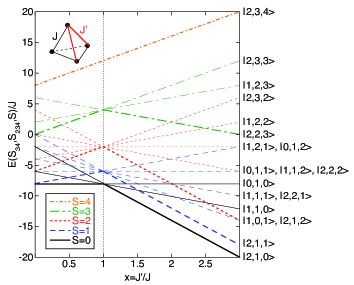
Figure 12: (Color online) Energy levels of $S=1$ tetramers calculated from Eq. (72) with $J<0$. The lowest states of a given $S$ value are marked by bold lines. The $|S_{34}S_{234}S\rangle$ states are identified at the right hand side. The insert shows the coupling parameters in a slightly distorted tetrahedron as realized for the compound {Ni₄Mo₁₂}.

Figure 12 displays the energy levels $E(S_{34},S_{234},S)$ normalized to $J$ (assuming AFM coupling $J<0$) as a function of the ratio $x=J^{\prime}/J$. For $x=1$ the energy levels are degenerate with respect to the total spin $S$, and the energy splittings follow the Landé rule Eq. (49). By applying a magnetic field the ground state changes in steps from $S=0$ to $S=4$ for the field values corresponding to the maxima of the $dM/dH$ data displayed in Fig. 11.

INS spectra measured for a polycrystalline sample of {Ni₄Mo₁₂} are shown in Fig. 13, from which two ground-state transitions can be identified at ca. 0.5 and 1.7 meV Nehrkorn et al. (2010). The former is composed of two subbands at 0.4 and 0.6 meV attributed to a ZFS from magnetic anisotropy. An excited-state transition appears at 1.2 meV. From Fig. 12 we can readily conclude that the singlet $|2,1,0\rangle$ has to be the ground state. Moreover, the first-excited state has to be the triplet $|2,1,1\rangle$ centered at 0.5 meV, since transitions between $S=0$ states are not allowed. The observed splitting of the triplet $|2,1,1\rangle$ into two components can be ascribed to an axial single-ion anisotropy defined by Eq. (10), which has the effect to split the states $|S_{34}S_{234}S\rangle$ into the states $|S_{34}S_{234}SM\rangle$. A least-squares fit to the energy spectra of Fig. 13 on the basis of the Hamiltonians Eq. (71) and (10) converged to the parameters $J=-0.25(2)$ meV, $J^{\prime}=-0.53(4)$ meV, $D=0.22(5)$ meV Furrer et al. (2010) which nicely reproduce the high-field magnetization data, see Fig. 11. The resulting low-energy splitting pattern is sketched in the insert of Fig. 13.

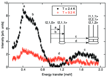
Figure 13: (Color online) Energy spectra of neutrons scattered from polycrystalline {Ni₄Mo₁₂} with an incident neutron energy of 3.27 meV. The insert attributes the observed transitions to the low-energy part of the splitting pattern. Adapted from Nehrkorn et al., 2010.

III.3.2 Pressure dependence of exchange parameters

By using external pressure the exchange parameters $J$ can be determined for varying distance $R$ between the magnetic ions. This is of importance for testing and improving theoretical models of the exchange interaction, where the distance usually enters in a straightforward manner. A detailed understanding of the exchange interaction is, for instance, indispensable for the engineering of spintronics devices made of magnetic semiconductors. In an effort to shed light on this issue the pressure dependence of $J$ was investigated for antiferromagnetically coupled Mn²⁺ dimers in the semiconducting compound Mn_0.02Zn_0.98Te Kolesnik et al. (2006). The corresponding energy-level scheme is indicated in Fig. 8. INS experiments performed for pressures of $p=0$ and $p=0.4$ MPa gave evidence for an appreciable pressure-induced upward shift of the observed dimer excitations as illustrated for the $|2\rangle\rightarrow|1\rangle$ transition with energy $4|J|$ in Fig. 14. The pressure-induced change of $J$ amounts to $dJ=-0.040(9)$ meV, accompanied by a 0.49% decrease of the intra-dimer distance $R$, resulting in a linear distance dependence $|dJ/dR|=1.8(4)$ meV/Å for $dR\ll R$. Similar INS experiments performed for CsMn_0.28Mg_0.72Br₃ gave evidence for a much stronger distance dependence of $J$ with $|dJ/dR|=3.6(3)$ meV/Å Strässle et al. (2004).

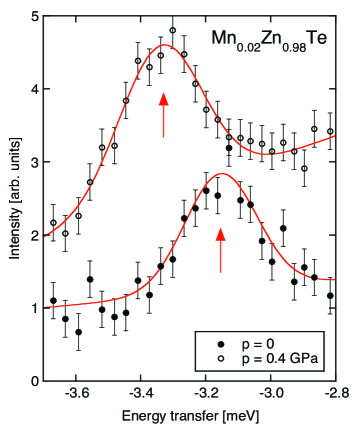
Figure 14: (Color online) Pressure dependence of the $|2\rangle\rightarrow|1\rangle$ transition associated with Mn²⁺ dimers in Mn_0.02Zn_0.98Te measured by INS. The lines denote Gaussian fits to the data. Adapted from Kolesnik et al., 2006.

III.3.3 Doping dependence of exchange parameters

It has been shown that a magnetic semiconductor can be converted by hole doping from its intrinsic AFM state to a ferromagnet Ferrand et al. (2001). It is still an open question whether the holes are localized or itinerant. The doping dependence of the exchange parameters may shed light on this issue. Neutron spectroscopic measurements were performed for single crystals of Mn_xZn_1-xTe, one with $x=0.05$ and doped with P to a level of 5$\times$10¹⁹ cm^-3, and another undoped reference sample with $x=0.02$ Kepa et al. (2003). The experiments were similar as those described in Sec. III.3.2 and gave evidence for a distinct doping-induced downward shift of the observed Mn²⁺ dimer excitations as illustrated for the $|2\rangle\rightarrow|1\rangle$ transition with energy $4|J|$ in Fig. 15. The doping-induced change of the exchange energy $J$ amounts to $dJ=0.013(3)$ meV, in reasonable agreement with $dJ=0.010$ meV calculated from the RKKY interaction which indicates that the ferromagnetic exchange is mediated by weakly localized holes.

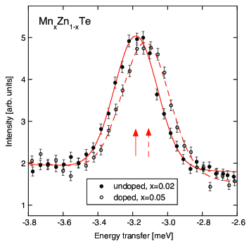
Figure 15: (Color online) Doping dependence of the $|2\rangle\rightarrow|1\rangle$ transition associated with Mn²⁺ dimers in Mn_xZn_1-xTe measured by INS. The lines denote Gaussian fits to the data. Adapted from Kepa et al., 2003.

III.3.4 Anisotropic exchange interactions

Exchange anisotropy can generally be expected for type-L and type-J compounds where orbital degeneracy is present. This is exemplified here for the type-L compound K₁₀[Co₄(D₂O)₂(PW₉O₃₄)₂]$\cdot$20D₂O which contains a tetrameric Co²⁺ cluster as sketched in Fig. 16. The combined action of spin-orbit and crystal-field interactions splits the ⁴T₁ single-ion ground state of the Co²⁺ ions into six anisotropic Kramers doublets Carlin (1986). By considering only the lowest single-ion level, an effective spin Hamiltonian of the Co²⁺ tetramer with $s=1/2$ for all ions can be written as

$$\hat{H} = -2J[\hat{s}_{1,x}\hat{s}_{3,x}+\hat{s}_{1,x}\hat{s}_{4,x}+\hat{s}_{2,x}\hat{s}_{3,x}+\hat{s}_{2,x}\hat{s}_{4,x}$$ (73)

$$+\hat{s}_{1,y}\hat{s}_{3,y}+\hat{s}_{1,y}\hat{s}_{4,y}+\hat{s}_{2,y}\hat{s}_{3,y}+\hat{s}_{2,y}\hat{s}_{4,y}$$

$$+\alpha(\hat{s}_{1,z}\hat{s}_{3,z}+\hat{s}_{1,z}\hat{s}_{4,z}+\hat{s}_{2,z}\hat{s}_{3,z}+\hat{s}_{2,z}\hat{s}_{4,z})]$$

$$-2J^{\prime}(\hat{s}_{1,x}\hat{s}_{2,x}+\hat{s}_{1,y}\hat{s}_{2,y}+\alpha^{\prime}\hat{s}_{1,z}\hat{s}_{2,z}).$$

It turns out that for this particular system the eigen functions are approximately given by the spin functions $|S_{12}S_{34}SM\rangle$ constructed through the spin coupling scheme $\hat{\bf S}_{12}=\hat{\bf s}_{1}+\hat{\bf s}_{2}$, $\hat{\bf S}_{34}=\hat{\bf s}_{3}+\hat{\bf s}_{4}$, $\hat{\bf S}=\hat{\bf S}_{12}+\hat{\bf S}_{34}$, with less than 1% $S$-mixing.

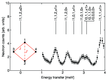
Figure 16: (Color online) Energy spectrum of neutrons scattered from K₁₀[Co₄(D₂O)₂(PW₉O₃₄)₂]$\cdot$20D₂O at $T=1.7$ K. The inserts show a sketch of the tetrameric Co²⁺ unit and the resulting energy level scheme, labeled with the dominant component $|S_{12}S_{34}S,\pm M\rangle$ of the wave function. The highest states $|1,1,1,0\rangle$ and $|1,1,0,0\rangle$ located at 5.04 and 5.79 meV, respectively, are not shown. Adapted from Clemente et al., 1997.

INS experiments gave evidence for well defined transitions associated with the Co²⁺ tetramer as shown in Fig. 16 Clemente et al. (1997). The data analysis based on Eq. (73) provided the exchange parameters $J=0.52$ meV, $\alpha=2.4$, $J^{\prime}=0.11$ meV, and $\alpha^{\prime}=4.6$, resulting in the energy level scheme indicated in Fig. 16. Both interactions $J$ and $J^{\prime}$ are ferromagnetic, thus leading to an $M=\pm 2$ ground state, in agreement with magnetic susceptibility and EPR experiments Gomez-Garcia et al. (1992). The exchange anisotropy is rather large as expected from the anisotropy of the Landé $g$ matrix with components in the range 2.6-7.0 observed by EPR experiments.

III.3.5 Higher-order single-ion anisotropies

Anisotropy-induced ground-state level splittings are essential to understand the step-like magnetic hysteresis curves and the related relaxation and spin reversal phenomena observed in the single-molecule magnets (see Sec V). EPR is the experimental tool of choice to determine ground-state level splittings, but because of the typically large ZFS parameters $D$ high magnetic fields and/or high frequencies are needed to obtain sufficiently resolved spectra. INS experiments offer a valuable alternative in zero field which will be demonstrated here for the tetrameric iron compound Fe₄(OCH₃)₆(dpm)₆, or Fe₄ in short, which has an $S=5$ ground state and shows slow relaxation of the magnetization below 1 K Barra et al. (1999). The four iron atoms lie exactly in a plane, with the inner Fe atom being in the center of an isosceles triangle. EPR experiments Bouwen et al. (2001) have shown that the single-ion anisotropies defined by Eqs. (10) and (11) are not sufficient to reproduce the observed signals in the ground-state multiplet, but higher-order anisotropy terms as given in Eq. (12) are needed. The anisotropy parameters resulting from the EPR experiments are listed in Table 4.

Table 4: Anisotropy parameters determined for Fe₄ (isomer AA) by EPR Bouwen et al. (2001) and INS Amoretti et al. (2001) experiments.

	$D$ [$\mu$eV]	$E$ [$\mu$eV]	$B^{0}_{4}$ [$\mu$eV]	$B^{2}_{4}$ [$\mu$eV]	$B^{4}_{4}$ [$\mu$eV]
EPR	-25.5(2)	1.2(4)	-1.4(3)$\times$10-3	-1.0(4)$\times$10-2	-0.(4)$\times$10-4
INS	-25.3(2)	-2.5(2)	-1.5(3)$\times$10-3	-	-

It can be seen from Table 4 that $D$ is the dominant anisotropy parameter which splits the $S=5$ ground state into a sequence of five doublets ($M=\pm 5,\pm 4,\pm 3,\pm 2,\pm 1$) and a singlet ($M=0$) with energies $DM^{2}$ according to Eq. (10). The other anisotropy parameters produce a slight mixing of the $|M\rangle$ states and/or give rise to small energy shifts. Nevertheless, the relevant selection rule in INS experiments is retained with good accuracy as $\Delta M=\pm 1$, as demonstrated by the data displayed in Fig. 17 Amoretti et al. (2001). The decreasing energy spacing with decreasing energy transfer prevented the transition $|M=\pm 1\rangle\rightarrow|M=0\rangle$ to be resolved from the elastic line. The anisotropy parameters resulting from the INS experiments are listed in Table 4. The value of $E$ is twice that obtained by the EPR measurements. Small discrepancies between the parameters determined by INS and EPR are frequently observed and are probably due to the high magnetic fields used by the latter technique, producing a rather large Zeeman splitting so that a mixing of the ground and the excited spin multiplets cannot be neglected.

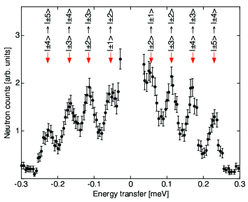
Figure 17: (Color online) Energy spectrum of neutrons scattered from Fe₄ at $T=6.5$ K . The transitions $|\pm M\rangle\rightarrow|\pm M^{\prime}\rangle$ within the $S=5$ ground-state multiplet are marked for each observed peak. Adapted from Amoretti et al., 2001.

III.3.6 Dzyaloshinski-Moriya interactions

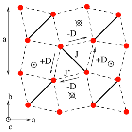
Figure 18: (Color online) Structural arrangement of the Cu²⁺ dimers (red balls connected with black lines) in SrCu₂(BO₃)₂ including the Dzyaloshinski-Moriya interactions whose vectors are perpendicular to the ($a$,$b$)-plane. The arrows show the order of the spins in the expression ${\bf d}(\hat{\bf s}_{i}\times\hat{\bf s}_{j})$. Adapted from Cépas et al., 2001.

The compound SrCu₂(BO₃)₂ is a two-dimensional spin-gap system with tetragonal unit cell. It consists of alternately stacked Sr and CuBO₃ planes. The latter are characterized by a regular array of mutually perpendicular Cu²⁺ dimers ($s=1/2$) as illustrated in Fig. 18. The gap associated with the singlet-triplet dimer excitations was determined by INS experiments to be 3.0 meV Kageyama et al. (2000). An almost perfect center of inversion at the middle of the dimer bonds forbids the Dzyaloshinski-Moriya (DM) interaction [Eq. (5)] between the two spins of a dimer. However, each dimer is separated from the neighboring dimer by a BO₃ unit, for which there is no center of inversion, so that the DM interaction is allowed between the next-nearest-neighbor (nnn) Cu²⁺ spins as described by the Hamiltonian

$$\hat{H} = \sum_{nnn}\pm d{\bf e}_{c}\cdot\left(\hat{\bf s}_{i}\times\hat{\bf s}_{j}\right)$$ (74)

where the sign depends on the bond (see Fig. 18), and ${\bf e}_{c}$ is the unit vector in the $c$ direction Cépas et al. (2001). The effect of Eq. (74) is to split the $\Delta M=\pm 1$ transition associated with the singlet-triplet splitting into four branches under the application of a magnetic field parallel to the $c$ axis. This prediction was verified by EPR measurements Nojiri et al. (1999) and later confirmed by INS experiments Cépas et al. (2001) as shown in Fig. 19. In addition to the four $\Delta M=\pm 1$ branches, the field-independent $\Delta M=0$ transition was observed in the INS measurements. The DM parameter resulting from these investigations turned out to be $d\approx 0.18$ meV, which roughly compares with the estimated value $d=(\Delta g/g)J_{nnn}\approx 0.5$ meV.

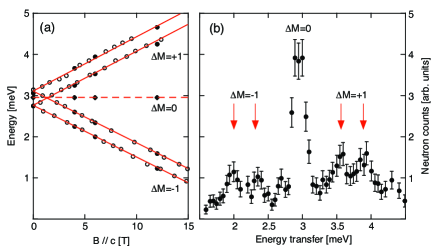
Figure 19: (Color online) (a) Magnetic field dependence ($B||c$) of the singlet-triplet excitations observed in SrCu₂(BO₃)₂ by EPR (open dots) and INS (solid dots) experiments. (b) INS spectrum of SrCu₂(BO₃)₂ at ${\bf Q}=(1,0,0)$ and $B=6$ T ($B||c$). Adapted from Nojiri et al., 1999 and Cépas et al., 2001.

III.3.7 A novel tool for local structure determination

Conventional crystallography is the standard tool for structure determination, and a periodic lattice is a prerequisite for such studies. However, complex materials are often characterized by local deviations from perfect periodicity which may be crucial to their properties. The most prominent bulk methods for local structure determination are x-ray absorption fine structure, nuclear magnetic resonance, and atomic pair-distribution function analysis. All these methods provide a spatial resolution of typically 0.1 Å, and their performance can hardly be improved. Magnetic cluster excitations are able to push the spatial resolution beyond the present limits through the dependence of the exchange coupling $J$ on the interatomic distance $R$, which for most materials is governed by the linear law $dJ/dR=\alpha$ as long as $dR\ll R$. Modern spectroscopies measure exchange couplings with a precision of $dJ/J\approx 0.01$, thus spatial resolutions of $dR\approx 0.01$ Å can be achieved as demonstrated below.

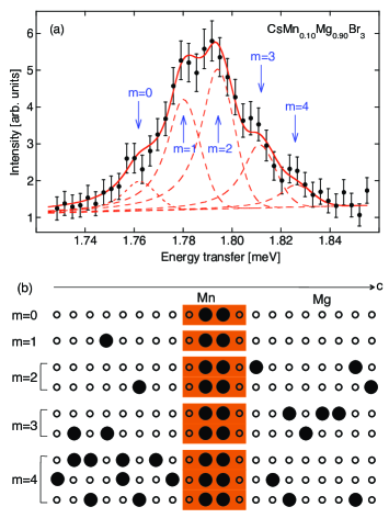
Figure 20: (Color online) (a) Energy distribution of the $|S=0,M=0\rangle\rightarrow|S=1,M=1\rangle$ Mn²⁺ dimer transition observed for CsMn_0.1Mg_0.9Br₃ at $T=1.6$ K. (b) Sketch of statistical distributions on Mn²⁺ and Mg²⁺ ions along the $c$ axis. $m$ is the number of Mn²⁺ ions replacing Mg²⁺ ions outside the central Mn²⁺ dimer embedded in the brown area. Adapted from Furrer et al., 2011b.

Table 5: Analysis of the INS spectrum of CsMn_0.1Mg_0.9Br₃ given in Fig. 20(a). $E_{m}$ and $I^{obs}_{m}$ denote the energy transfers and the normalized intensities of the individual bands $m$, respectively. The intensities $I^{calc}_{m}$ were calculated according to a statistical model described in Furrer et al., 2011b. Relative error bars are given for the exchange couplings $J_{m}$ and for the local Mn-Mn distances $R_{m}$.

m	$E_{m}$ [K]	$I^{obs}_{m}$	$I^{calc}_{m}$	$J_{m}$ [meV]	$R_{m}$ [Å]
0	1.762(2)	0.081(22)	0.119	-0.8321(10)	3.2311(3)
1	1.780(2)	0.302(25)	0.289	-0.8408(10)	3.2287(3)
2	1.794(2)	0.383(22)	0.310	-0.8477(10)	3.2268(3)
3	1.811(2)	0.173(22)	0.193	-0.8563(10)	3.2244(3)
4	1.826(3)	0.061(18)	0.089	-0.8637(14)	3.2224(4)

We turn to Fig. 10 which displays Mn²⁺ dimer excitations in CsMn_xMg_1-xBr₃. The total linewidths of the transitions A and B show an $x$-dependent increase beyond the instrumental energy resolution (FWHM = 55 $\mu$eV) which was further investigated by high-resolution INS experiments with FWHM = 15 $\mu$eV Furrer et al. (2011b). As shown in Fig. 20(a), the energy spectrum observed for the transition A exhibits marked deviations from a normal Gaussian distribution. It is best described by the superposition of five individual bands which correspond to specific Mn²⁺ dimer configurations with particular exchange couplings $J_{m}$ ($m=0,1,2,3,4$). The linear law $dJ/dR=\alpha$ was established for CsMn_xMg_1-xBr₃ with $\alpha=3.6$ meV/Å Strässle et al. (2004), thus each of the five $J_{m}$ values can be associated with a particular local distance $R_{m}$ as listed in Table 5.

How can the discrete nature of the local Mn-Mn distances be explained? In Fig. 20(b) different configurations along the Mn chain structure are sketched, where $m$ is the number of peripheral Mn²⁺ ions replacing the Mg²⁺ ions. The introduction of additional Mn²⁺ ions exerts some internal pressure within the chain, since the ionic radii of the Mn²⁺ (high spin) and Mg²⁺ ions are different with $r_{Mn}=0.83$ Å$>r_{Mg}=0.72$ Å Shannon (1976), so that the atomic positions have to rearrange. In particular, the Mn-Mn bond distance of the central Mn²⁺ dimer is expected to shorten gradually with increasing number of Mn²⁺ ions as compared to the case $m=0$. For any number $m$ there is a myriad of structural configurations, resulting in a continuous distribution of local distances $R_{m}$. This view, however, is in contrast to the observed energy spectrum displayed in Fig. 20(a) which is clearly not continuous. In other words, the bond distance is not smoothly adjusted to its surrounding but locks in at a few specific values $R_{m}$. Obviously the realization of discrete local distances $R_{m}$ is governed by the number $m$ of peripheral Mn²⁺ ions and not by their specific arrangement in the chain. This surprising result is due to the one-dimensional character of the compound CsMn_xMg_1-xBr₃ in which the mixed Mn_xMg_1-x chains behave like a system of hard core particles Krivoglaz (1996). In conclusion, the use of high-resolution spectroscopies allows a rather direct determination of local interatomic distances in small magnetic clusters, in contrast to other techniques which usually have to be combined with simulations.

IV Large magnetic clusters

IV.1 Introduction

In the previous section, the scientific questions addressed by the small magnetic clusters focused on demonstrating and elucidating the nature of the various basic interactions between the spin centers in condensed matter systems. However, in large magnetic clusters, or the molecular nanomagnets in the context of this review, the huge size of the Hilbert space makes a complete experimental characterization of the magnetic cluster excitations (usually) impossible. Accordingly, the fine details in the spin interactions such as exchange anisotropy are not detected, and the modeling of the data can with much success be based on spin models taking into account only the dominant interactions, which in most cases is Heisenberg exchange. The spectroscopic experiments typically reveal the low-lying excitations or the low-energy sector of these spin models, and one is hence naturally directed towards questions such as what is the nature of the ground state and elementary excitations.

The key distinguishing feature as compared to the previous section is the many-body structure of the wave-functions in the large magnetic clusters, and a main goal could be formulated as what novel quantum states are realized and which physical concepts allow us to rationalize them. At this point the close ties to the field of, e.g., quantum spin systems becomes apparent, and indeed methodologies developed there are often applied to molecular nanomagnets. Most of the examples presented in this section will elaborate on that.

However, also distinguishing novel aspects come into play as a consequence of the fact that the molecular nanomagnets are not extended. For instance, phase transitions, either classical or quantum, are not possible in a strict sense. Conceptually most important, however, is that the wave vector ${\bf q}$ ceases to be a useful quantum number. One can actually expect that exactly those lattice topologies which cannot be expanded into an extended lattice will exhibit the most interesting novel complex quantum states and magnetic phenomena. Research into this direction has just started, however, and only preliminary results are available at the time of the writing of this manuscript. A further important point not emphasized yet is that the spins of the magnetic centers in molecular nanomagnets are generally rather large, with $s_{i}=3/2,2,5/2$ being most often found, in contrast to quantum spin system, where much focus is on spin-1/2 systems. Typical metal ions would be Cr³⁺ and Mn⁴⁺ ($s_{i}=3/2$), Mn³⁺ ($s_{i}=2$), and Mn²⁺ and Fe³⁺($s_{i}=5/2$). The quantum-classical correspondence hence enters naturally in the discussion of the magnetic excitations in molecular nanomagnets.

In the following those classes of molecules will be discussed for which considerable insight into the magnetic cluster excitations has been obtained. Important classes such as odd-membered wheels Yao et al. (2006); Hoshino et al. (2009b); Cador et al. (2004), ferromagnetic clusters Clemente-Juan et al. (1999); Low et al. (2006); Stuiber et al. (2011), discs Hoshino et al. (2009a); Koizumi et al. (2007), and others are not mentioned.

An important subclass of molecular nanomagnets are the single-molecule magnets (SMMs), which have received the largest attention in the past and could be described as having given birth to the molecular nanomagnets as a research field. The above questions are also relevant, but the most interesting phenomena in SMMs, such as quantum tunneling of magnetization, are mainly related to magnetic anisotropy. The SMMs will be discussed in Sec. V.

IV.2 Theoretical description

IV.2.1 Spin Hamiltonian

As mentioned before, experimental results on large magnetic clusters can often very well be reproduced by spin Hamiltonians which include only the most dominant terms. For clusters containing only type S and Q metal ions, on which we focus in this review, these are the HDVV Hamiltonian Eq. (2), the single-ion anisotropy Eqs. (10) and (11), and the Zeeman term Eq. (13). However, in molecular nanomagnets the site symmetries of the individual spin centers in the cluster are very low, if they have symmetry at all. Accordingly, the single-ion anisotropy and $g$ factors should in general be described as tensors. Also, in molecular nanomagnets often different kinds of metal centers are incorporated. This gives rise to the spin Hamiltonian

$$\hat{H} = -2\sum_{i<j}J_{ij}\hat{\bf{s}}_{i}\cdot\hat{\bf{s}}_{j}+\sum_{i}\hat{\bf{s}}_{i}\cdot{\bf D}_{i}\cdot\hat{\bf{s}}_{i}$$ (75)

$$+\mu_{B}\sum_{i}\hat{\bf{s}}_{i}\cdot{\bf g}_{i}\cdot{\bf B},$$

which in the following will be referred to as microscopic Hamiltonian in order to clearly distinguish it from effective models which also appear. The dipole-dipole interaction Eq. (4) has also to be included, but its effect on energy spectrum and magnetic behavior is very similar to that of the single-ion anisotropy term and may hence be lumped into the single-ion parameters. Experimental $D$ and $E$ values which were derived with the dipole-dipole interaction explicitly included in Eq. (75) will be indicated by a superscript ”lig”.

In contrast to the sites, the molecule itself may exhibit, or closely approximate, a high molecular symmetry. In fact, clusters with a particular symmetry are appealing for physical studies, and are thus preferred objects of investigations. The microscopic Hamiltonian simplifies then enormously and includes only few parameters.

Usually the HDVV Hamiltonian dominates over the single-ion anisotropy, and the strong-exchange limit (Sec. II.1) is an excellent starting point. Although the magnetic anisotropy cannot be ignored in the analysis of experimental data, the physics of interest in these cases is (usually) related to the Heisenberg interactions, and the discussion focuses on the corresponding Heisenberg spin models (notable exceptions are the SMMs discussed in Sec. V). The magnetic anisotropy may however also be so large that important effects appear which are not covered by the strong-exchange limit ($S$ mixing)Liviotti et al. (2002); Waldmann and Güdel (2005) or may need completely different physical concepts for their description. The examples selected below will demonstrate this point. It is added that from the values of magnetic parameters, such as $J$ and $D$, it is usually not possible to infer a priori whether the strong-exchange limit is obeyed or not. The ratio $D/J$ is generally small in molecular nanomagnets, and which case is realized needs a case-to-case analysis.

The dimension of the Hilbert spaces encountered in large magnetic clusters poses a major obstacle, similar to that found in other areas such as quantum spin systems, and the same conceptual ideas are followed to tackle it. Indeed, essentially any technique developed in the context of quantum spin systems is also of interest for large magnetic clusters. However, some of them had been of particular use, and are mentioned next.

IV.2.2 Numerical techniques

A most straight forward approach is to numerically solve the spin Hamiltonian for its energies and eigen functions, which is achieved in two steps, setting up the Hamiltonian matrix and then diagonalizing it.

The major decision in the first step is the choice of the basis set, which could be the product states $|\{M_{i}\}\rangle$ (with an obvious shorthand notation) or the spin functions $|\eta SM\rangle$, where $\eta$ denotes the intermediate spin quantum numbers generated in a particular spin coupling scheme. The product states are most easily handled in computer code, yield sparse Hamiltonian matrices, and are eigenfunctions of $\hat{S}_{z}$ which allows a block factorization for magnetic clusters with uniaxial symmetry. On the other hand, for the spin functions it is numerically demanding to calculate matrix elements (a number of Wigner symbols need to be calculated) and the matrices are dense, but they have the intrinsic advantage of being eigenfunctions of the total spin operator $\hat{\bf S}$ which results in a very effective block-factorization for the HDVV Hamiltonian. Interestingly, nearly all numerical work in the field of quantum spin systems has been based on product states; spin functions are rarely used. However, for large magnetic clusters diagonalization using spin functions has been used with much success Delfs et al. (1993); Waldmann et al. (1999); Guidi et al. (2004); Baran et al. (2008), and efficient ITO based techniques have been developed for calculating matrix elements Gatteschi and Pardi (1993) and employing spatial symmetries Waldmann (2000); Schnalle and Schnack (2010).

Complete information on the system is obtained by a full exact diagonalization, and several canned computer codes are available Bai et al. (2000). The largest dimension of the Hilbert space which can be handled is ca. 100 000 on a super computer, or about 15 000 on a (32 bit) personal computer. If symmetries are systematically taken into account, quite large magnetic clusters can be treated on personal computers, e.g., a mixed valent Mn-[3$\times$3] grid molecule with a Hilbert space dimension of 4 860 000 Waldmann et al. (2006c).

If full exact diagonalization is not possible, one may attempt to obtain the energies and eigen functions in a subspace. A first approach is to truncate the space of basis function, but the success of the procedure obviously depends on how well the selected basis states represent the sought-after eigen functions Schnalle and Schnack (2009).

A set of very efficient diagonalization methods is given by the sparse matrix diagonalization techniques, which allow an exact numerical calculation of a small number ($\sim$100) of selected energies and/or eigen states, typically the low-lying states Bai et al. (2000). In physics the most prominently used variant is the Lanczos method, while in chemistry the Jacobi-Davidson algorithm is more often applied. However, for the specific purpose of calculating the low-temperature observables of large magnetic clusters, the simpler subspace-iteration techniques turn out to be quite powerful, since they provide both energies and eigen function even in the presence of degeneracies with very comparable convergence rates.

These techniques employ an iterative process and work best for sparse matrices. Because of the latter it is most natural to use the product states, though spin functions were applied in few cases Guidi et al. (2004). The iterative process consists of repeatedly applying the Hamiltonian matrix $\bf H$ to a vector $\bf x$,

$${\bf x}_{n+1}=({\bf H}-\sigma{\bf 1})\cdot{\bf x}_{n},$$ (76)

where $\sigma$ introduces a shift which allows to optimize the convergence rate, and the starting vector ${\bf x}_{0}$ may be a random vector. If more than one eigen pair is searched, the iteration is applied to a subspace of vectors $\bf X$. For a practical algorithm, some further improvements are suggested Bai et al. (2000). The Lanczos and Jacobi-Davidson algorithms are also based on matrix-vector multiplications ${\bf H}\cdot{\bf x}$, but employ more sophisticated algorithms to extract the information on the eigen pairs from the generated vectors Bai et al. (2000).

Besides these approaches a number of numerical techniques exist which aim at calculating observables directly without evaluating eigen pairs explicitly. Among these are e.g. Quantum Monte Carlo, Chebyscheff expansion, dynamic and finite-temperature Lanczos, transfer matrix and (dynamical) density matrix renormalization group methods. However, although promising, these methods have not yet been applied systematically to the analysis of large magnetic clusters as defined in this review, but few applications were reported Exler and Schnack (2003); Engelhardt et al. (2006); Torbrügge and Schnack (2007); Schnack and Wendland (2010); Ummethum et al. (2012). More efforts in this direction would obviously be desirable.

IV.2.3 Effective Hamiltonian techniques

Another approach to describe the relevant low-energy excitations in a particular spin model is to replace the microscopic Hamiltonian by an effective spin Hamiltonian (mapping), which acts in a Hilbert space of (significantly) reduced dimension. It is emphasized that the states in the Hilbert space of the effective Hamiltonian do not have to be identical to those of the microscopic Hamiltonian. An effective Hamiltonian may be constructed from various procedures, but the following simple technique had been particularly useful for rationalizing the magnetism in a number of large magnetic clusters.

The method can be described as a first-order perturbation treatment, as integrating out a degree of freedom or as a mean-field argument and is guided by physical intuition. It starts with combining a subset of the spins $\hat{\bf s}_{i}$ in a collective spin $\hat{\bf S}_{\mu}=\sum_{i\in\mu}\hat{\bf s}_{i}$, where $\mu$ stands for the set of sites $i$, and selecting the sector of interest via the value of the quantum number $S_{\mu}$ associated to $\hat{\bf S}_{\mu}$, which is usually the minimal or maximal value. Then it holds

$$\hat{\bf s}_{i}=c_{i}\hat{\bf S}_{\mu},$$ (77)

with a projection coefficient $c_{i}$, which depends on $s_{i}$ and $S_{\mu}$. For the sector where all spins in the subset $\mu$ are ferromagnetically aligned and $S_{\mu}$ assumes its maximal value $S_{\mu}=\sum_{i}s_{i}$ holds $c_{i}=s_{i}/S_{\mu}$. The effective Hamiltonian is then finally obtained by inserting Eq. (77) in the microscopic Hamiltonian, which removes the spins $\hat{\bf s}_{i}$ of the subset $\mu$ and replaces them by the collective spin $\hat{\bf S}_{\mu}$.

A typical situation where the above scheme could be applied is a cluster with one or few ferromagnetic exchange couplings which are much larger than the other ones. Then the spins linked by a strong ferromagnetic coupling can be combined into one collective spin which replaces them in the spin Hamiltonian. Another situation is an antiferromagnetic bipartite lattice, where the spins on each sublattices $A$ or $B$ are ferromagnetically aligned with respect to each other in the ground state. This suggests to introduce two sublattice spins $\hat{\bf S}_{A}$ and $\hat{\bf S}_{B}$, and to transform the Hamiltonian according to Eq. (77). The subsections below will provide examples for the practical application of the scheme.

IV.2.4 Condensed matter techniques

Sophisticated techniques for calculating properties of extended (quantum) spin systems have been developed. Some of them can directly be applied to large magnetic clusters as they work for any number $N$ of spin centers, i.e., the thermodynamic limit is not assumed a priori but taken after completion of the calculation. However, in magnetic clusters translational invariance is not present, and it is hence a characteristic feature of the application of these techniques to clusters that they have to be adapted to work in real space and not momentum space as in extended systems, which may bring in novel aspects. This area is still largely unexplored, but two of the simpler techniques in this class of methods have been applied with some success. They both elaborate on the observation that in molecular nanomagnets the spins $s_{i}$ are relatively large.

Spin-wave theory (SWT), or the set of techniques embraced by this acronym such as linear SWT, interacting SWT, or modified and finite-size SWT Rado and Suhl (1963); Ivanov and Sen (2004); Takahashi (1987); Hirsch and Tang (1989); Zhong and Sorella (1993), is certainly a most successful theory in magnetism. All variants have in common that they start from a classical spin configuration in the ground state, and expand around it by approximating the single-site spin operators $\hat{\bf s}_{i}$. They are hence semi-classical in nature, and - technically - can be applied to any type of lattice, and in particular to large magnetic clusters when formulated in real space Cépas and Ziman (2005). It is necessary to distinguish between SWTs for ferromagnetic and antiferromagnetic clusters. For ferromagnetic clusters, SWT allows us to calculate the zero-temperature excitation spectrum exactly for any arbitrary cluster. However, since SWT breaks spin rotational invariance it is conceptually inappropriate for antiferromagnetic systems with disordered ground states, such as one-dimensional (1D) systems or magnetic clusters. Nevertheless, it is often found to produce significant results e.g. for excitation energies Ivanov and Sen (2004), but the reliability of the results should carefully be checked case-by-case. The fundamental questions as regards the applicability of SWT to antiferromagnetic clusters shall not be addressed in this review, but results of some few case-by-case checks will be reported. For the technical implementation of SWT for magnetic clusters we refer to Stuiber et al. (2011); Waldmann (2007).

The large spins in molecular nanomagnets suggest an entirely classical description, where each spin operator $\hat{\bf s}_{i}$ is replaced by a classical vector ${\bf s}_{i}$ of appropriate length, or a unit vector ${\bf e}_{i}$ times a prefactor $\tilde{s}_{i}$, ${\bf s}_{i}=\tilde{s}_{i}{\bf e}_{i}$. A subtlety arises here as regards the appropriate value of $\tilde{s}_{i}$, which can be argued to be best taken as $\tilde{s}_{i}=\sqrt{s_{i}(s_{i}+1)}$ Joyce (1967); Luscombe and Luban (1997) or $\tilde{s}_{i}=s_{i}$ Fisher (1964). With this replacement the Hamiltonian becomes a classical functional, and the ground-state energy and spin configuration is obtained by minimization. Also, thermodynamic quantities can be calculated for quite large magnetic clusters of hundreds of sites, and it is here where the classical approach was mostly applied to molecular nanomagnets Schröder et al. (2005a); Müller et al. (2001a); Yao et al. (2006). The calculation of dynamic quantities is also possible Luscombe and Luban (1997); Luscombe et al. (1998), but the discrete energies of the excitations in magnetic clusters can of course not be recovered, though their intensities Mentrup et al. (2000). Hence, the classical calculations are not actually suited to reproduce experimental spectroscopic data, but nevertheless can provide significant insight into the physics of the excitations in a large magnetic cluster through the quantum-classical correspondence Schröder et al. (2005b), which is probably the most important aspect.

IV.3 Even-membered antiferromagnetic molecular wheels

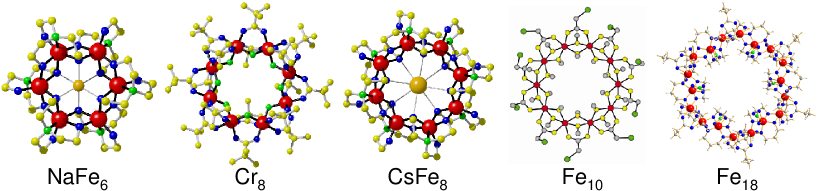
Figure 21: (Color online) Molecular structures of the five even-membered antiferromagnetic wheels NaFe₆: Na[Fe₆tea₆]Cl, Cr₈: [Cr₈F₈Piv₁₆], CsFe₈: Cs[Fe₈tea₈]Cl, Fe₁₀: [Fe₁₀(OCH₃)₂₀(O₂CCH₂Cl)₁₀], and Fe₁₈: [Fe₁₈(pd)₁₂(pdH)₁₂(O₂CEt)₆(NO₃)₆].

Molecular wheels are species in which the metal ions form almost perfect ring-like structures. The decanuclear wheel [Fe₁₀(OCH₃)₂₀(O₂CCH₂Cl)₁₀], or Fe₁₀ in short, was the first wheel whose magnetic properties were studied Taft et al. (1994); Gatteschi et al. (1994). Since then, because of their aesthetical appeal and unprecedented magnetism, the class of the molecular wheels has enormously grown and dozens of wheels with nuclearity ranging from $N=6$ to $N=18$ have been synthesized. In Fig. 21 the crystal structures of five representatives are displayed. The physics in the molecular wheels, and their relatives such as the modified wheels (Sec. IV.4), turned out to be surprisingly rich. The presentation here is hence necessarily limited.

The even-membered antiferromagnetic wheels have been the subject of intense research. In this section, homo-nuclear wheels will be discussed with $s_{i}=s$ for all $i$. In view of the high molecular symmetry, which in hexa-nuclear wheels can be a crystallographic S₆ symmetry and in octa-nuclear wheels a C₄ symmetry, the magnetism should be expected to be very well described by the generic spin Hamiltonian

$$\hat{H} = -2J\left(\sum_{i=1}^{N-1}\hat{\bf{s}}_{i}\cdot\hat{\bf{s}}_{i+1}+\hat{\bf{s}}_{N}\cdot\hat{\bf{s}}_{1}\right)$$ (78)

$$+D\sum_{i}\left[\hat{s}_{iz}^{2}-\frac{1}{3}s_{i}(s_{i}+1)\right]+\mu_{B}g\hat{\bf{S}}\cdot{\bf B}.$$

Additional terms describing e.g. a variation of the exchange constants along the wheel, tilted single-site anisotropy tensors or higher-order terms should in principle also be present, but these are difficult to resolve in experiment. Sometimes a planar term $E\sum_{i}(\hat{s}_{ix}^{2}-\hat{s}_{iy}^{2})$ had to be added to Eq. (78) (vide infra), and evidence for weak Dzyaloshinski-Moriya interactions were reported Cinti et al. (2002); Lante et al. (2009). However, the latter manifests itself only in very specific experiments, and is not further considered. The Hamiltonian Eq. (78) (plus sometimes an $E$ term) generally provides a very good description.

The exchange coupling $2J$ is typically on the order of few meV, and the single-ion anisotropy weak, $|D|<0.1$ meV. In most cases it is of the easy-axis type ($D<0$), with the exception of Fe₁₈, where $D>0$ (vide infra). The ratio $D/J$ is small in the antiferromagnetic wheels, but the strong-exchange limit is not necessarily well obeyed. In fact, the effect of the anisotropy is rather determined by $(Ns)^{2}|D/J|$ Chiolero and Loss (1998); Waldmann (2002a), and antiferromagnetic wheels should be classified according to wether the anisotropy is ”weak” or ”strong” by the different physics in the two limits.

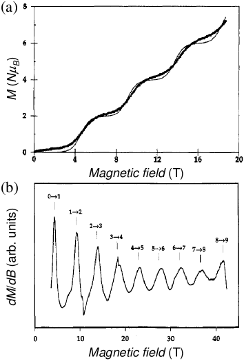
Figure 22: (a) Magnetization vs field and (b) differential magnetization $dM/dB$ at a temperature of 0.6 K of the antiferromagnetic wheel Fe₁₀. The data show the sequence of magnetization steps, which were be traced here for fields up to 40 T. Adapted from Taft et al., 1994.

The magnetic susceptibility data have conclusively pointed towards a $S=0$ ground state in the antiferromagnetic wheels, which is intuitively anticipated from the expected alternating up and down spin configuration in the classical ground state. The first general insight into the excitation spectrum has been obtained from low-temperature magnetization curves on the Fe₁₀ wheel, which are reproduced in Fig. 22. A sequence of magnetization steps is seen as function of field, where at each step the magnetization changes by 2 $\mu_{B}$, and which occur in regular field intervals of ca. 4.2 T. This demonstrates that as function of field the ground state changes from $S=0$ to $S=1$ at the first step, $S=1$ to $S=2$ at the second step, and so on, as sketched in Fig. 23. From the fields of the magnetization steps or ground-state level crossings one can infer the zero-field energies of the states Shapira and Bindilatti (2002), with the result

$$E(S)=\frac{\Delta}{2}S(S+1).$$ (79)

The excitation spectrum consists hence of a set of spin multiplets with $S=0,1,2,...$ whose energies satisfy the Landé rule Eq. (49), see also Fig. 23, where $\Delta$ is the energy gap between the singlet and triplet. Such a spectrum is also generated by a Heisenberg dimer $\hat{H}_{AB}=\Delta\hat{\bf S}_{A}\cdot\hat{\bf S}_{B}$, with appropriate spins $S_{A}$ and $S_{B}$. The Hamiltonian $\hat{H}_{AB}$ appears hence as an effective spin Hamiltonian for the antiferromagnetic Heisenberg model on a ring. There is however some deeper physics in here, which will be mentioned in the next subsection.

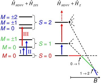
Figure 23: (Color online) Sketch of the low-lying energies in even antiferromagnetic molecular wheels. The Heisenberg interactions give rise to spin multiplets $S=0,1,2,\ldots$ which split in a magnetic field and lead to level crossings in the ground state, which changes from $|S=0,M=0\rangle$ to $|1,-1\rangle$, $|1,-1\rangle\rightarrow|2,-2\rangle$, etc., and steps in the magnetization curve. The magnetic anisotropy splits the spin multiplets in zero field, as indicated to the left. Some allowed INS transitions are indicated by arrows.

The role of magnetic anisotropy in antiferromagnetic wheels was elucidated by EPR Pilawa et al. (1997, 2001, 2003); van Slageren et al. (2002) and measurements of the magnetic torque Cornia et al. (1999a, b); Waldmann et al. (1999). The first INS experiment on a wheel was performed on the cluster Na[Fe₆{N(CH₂CH₂O)₃}₆]Cl, or NaFe₆ (Fig. 21) Waldmann et al. (1999). The experimental data are reproduced in Fig. 24, and are characterized by two cold transitions I and II, and a hot transition III. The interpretation of the observed transitions is straightforward: Peaks I and II correspond to transitions from the $S=0$ ground state to the zero-field-split $S=1$ multiplet, and peak III to a transition from the $|S=1,M=0\rangle$ level to the $S=2$ multiplet, as indicated in Fig. 23. The INS energies yield directly $2J=-2.0$ meV and $D=-0.038$ meV, in excellent agreement with magnetic susceptibility and magnetic torque measurements, which puts NaFe₆ in the ”weak” anisotropy category.

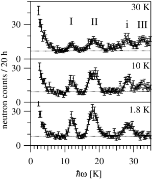
Figure 24: Neutron energy-loss spectrum of NaFe₆ at the indicated temperatures ($Q=1.0$ Å^-1). The transition i could be assigned to an impurity species in the sample. Adapted from Waldmann et al., 1999.

The following three subsections are organized by the ”strength” of the magnetic anisotropy or parameter $(Ns)^{2}D/J$. First, the physics in the ”weak” anisotropy case, which is that of the $L\&E$-band picture, is considered followed by the ”intermediate” anisotropy case. Finally, wheels with ”strong” anisotropy which may display quantum tunneling of the Néel vector are discussed.

IV.3.1 Antiferromagnetic wheels with ”weak” anisotropy and the $L\&E$-band picture

Most antiferromagnetic wheels fall into the weak anisotropy category. The anisotropy leads to a zero-field splitting of the spin multiplets, which is detected in e.g. INS experiments as was shown by the example of NaFe₆, but the physics of the magnetic excitations is not affected by it. Hence, the appropriate model for the discussion of the physics is that of the antiferromagnetic Heisenberg ring (AFMHR) or Eq. (78) with $D=0$.

Initially, the wheels were regarded as models for 1D antiferromagnetic chains with the implication that the physical concepts developed for them, which are characterized by the strong quantum fluctuations in 1D, should also apply to AFMHRs. However, the experimental and theoretical work has suggested a very different picture of the excitations, which is denoted here as $L\&E$-band concept. This concept has its roots in Anderson’s 1952 paper on antiferromagnetic spin waves Anderson (1952), and emerged in the course of several works Anderson (1984); Bernu et al. (1992); Caneschi et al. (1996); Chiolero and Loss (1998); Schnack and Luban (2000); Waldmann (2002b); Lhuillier (2002). The $L\&E$-band concept is classical in nature, though some subtleties are present, and the meaning of ”classical” in this context is in fact not yet completely understood. It rather seems that in magnetic clusters of the size discussed here the line between classical and quantum physics is blurred Konstantinidis et al. (2011). Fundamental questions hence remain. However, from a practical point of view the $L\&E$-band concept seems to apply whenever the classical spin structure appears to describe well the ground state, and has allowed rationalizing the magnetism in a number of different classes of molecules. The molecular wheel [Cr₈F₈Piv₁₆], or Cr₈ (Fig. 21), has played an important role in this context, as it was the first system for which a detailed, and indeed complete, experimental demonstration of the concept was achieved by exploiting the full power of INS.

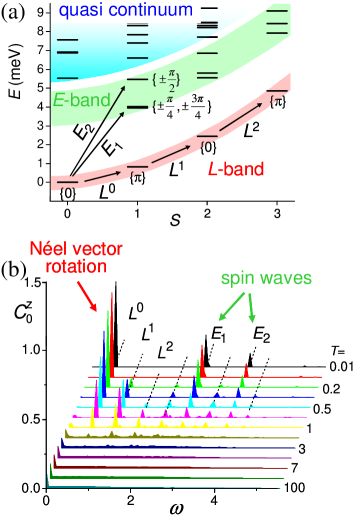
Figure 25: (Color online) (a) Simulated energy spectrum for a $N=8$, $s=3/2$ AFMHR with $2J=-1.46$ meV as for Cr₈. The low-lying levels form rotational bands. The $L$ band can be rationalized as (quantized) rotation of the Néel vector. The next higher-lying bands are denoted collectively as $E$ band and may be regarded as (discrete) antiferromagnetic spin waves. Some INS transitions are indicated by arrows with associated labels. The numbers in brackets indicate the shift quantum number $q$ for some spin multiplets. (b) Simulated spin-spin auto-correlation function $C^{z}_{0}(\omega)$ in units of $2|J|$ for various temperatures. The $L$- and $E$-band transitions indicated in panel (a) are identified. Adapted from Waldmann et al., 2003 and Waldmann, 2002b.

Descriptions of the $L\&E$-band concept are available Waldmann (2005a); only major aspects are mentioned here. The key ingredient is the notion of rotational bands, where a rotational band is a sequence of spin multiplets with $S=S_{min},S_{min}+1,S_{min}+2,...$ whose energies increase according to the Landé rule $E(S)\propto S(S+1)$. The analogy of this spectrum with that of a rigid rotator $\hat{H}=\hat{\bf L}^{2}/(2I)$, where $\hat{\bf L}$ is an angular momentum and $I$ the moment of inertia, is not coincidental. The $L\&E$-band concept can be summarized as:

(1) In an energy-vs-$S$ plot, the low-energy sector is characterized as a set of rotational modes; the lowest-lying mode called $L$ band and a number $n_{E}$ of higher-lying modes called $E$ band. The next higher-lying states are collectively denoted as quasi continuum.

(2) The classification of the energy states in (1) is justified by a selection rule: Spin transitions from the $L$ band into the quasi continuum are forbidden. Hence, at low temperatures only INS transitions between states of the $L$ band or from the $L$ to the $E$ band are allowed.

Importantly, these points have to come together Waldmann (2002b). The presence of a rotational mode is by itself not sufficient to ensure the validity of the $L\&E$-band concept and its consequences. In Fig. 25 are shown the energy spectrum and spin-spin auto-correlation function $C^{z}_{0}(\omega)$ of a $N=8$, $s=3/2$ AFMHR. The structure of the energies detailed in (1) is clearly seen. Also, the correlation function demonstrates, e.g., that transitions from the $S=0$ ground state into the quasi continuum do not occur. The above two points completely define the concept, but some further comments are at place:

$L$ band: The $L$ band is intimately related to the occurrence of long-range Néel order: For lattices which can be expanded to infinity, the presence of the $L$ band in the spectrum is a necessary but not sufficient requirement for an ordered Néel ground state in the infinite lattice Bernu et al. (1992). It is hence also related to the corresponding antiferromagnetic Goldstone mode, and the $L$-band states have spatial symmetries consistent with the ordered Néel state. An excellent discussion is found in Lhuillier, 2002. Qualitatively, the $L$ band reflects the rotational degree of freedom of the classical antiferromagnetic spin configuration in the ground state, or (quantized) rotation of the Néel vector. The $L$ band is also known as the tower of states or quasi-degenerate joint states.

$E$ band: The $E$ band is deeply related to spin waves: For lattices which can be expanded to infinity, the $E$ band evolves into the familiar antiferromagnetic spin waves in the infinite lattice (where we deviate from the usual notation by not regarding the Goldstone mode or antiferromagnetic Bragg peak as a spin wave, see Ref. 25 in Waldmann, 2007). In finite clusters, the spin-wave spectrum becomes of course discretized. It then consists of $n_{E}$ energies, and each of them corresponds to one of the $n_{E}$ rotational modes in the $E$ band. Although originating from extended lattices, the concept of spin waves can be carried over in an obvious manner to any lattice which obeys the $L\&E$ band concept, not only those characterized by a wave vector Cépas and Ziman (2005). Qualitatively, the $E$ band reflects the possible higher-energetic internal spin structures which results as excitations from the classical antiferromagnetic ground-state spin configuration.

In the AFMHR the cyclic symmetry gives rise to a shift quantum number $q$ defined via the shift operator $\hat{T}|q\rangle=e^{iq}|q\rangle$ with $q=0,\pm 2\pi/N,...,\pi$ by which the excitations can be classified. A complete theory is not existing but phenomenologically the energies of the $L$ and $E$ band for $S\geq 1$ can then be approximated by

$$E(S,q)=\frac{1}{2}\epsilon(\pi)S(S+1)+\epsilon(q)-\epsilon(0)$$ (80)

with $q=0,\pi$ for the $L$ band. $\epsilon(q)$ can be regarded as the finite-size version of the spin-wave dispersion relation Dreiser et al. (2010b). Indeed, in the infinite chain $q$ would become the wave vector, and $\epsilon(q)$ would agree with the familiar spin-wave dispersion Anderson (1952). However, it is emphasized again that the $L\&E$-band concept is not limited to clusters with cyclic or a similar high symmetry, it can also be observed in clusters with different point group symmetries or no symmetry at all (vide infra).

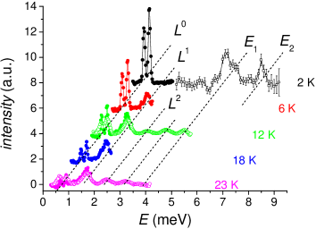
Figure 26: (Color online) Neutron energy-loss spectrum of Cr₈ at the indicated temperatures. Adapted from Waldmann et al., 2003.

We turn now to discussing the molecular wheel Cr₈. In this molecule, eight Cr³⁺ ions ($s=3/2$) form an almost perfect planar octagon. The system crystallizes in space group P42₁2, and the molecule nominally exhibits C₄ symmetry. However, disorder in some pivalate ligands and tBu groups is present, suggesting that the individual molecules are slightly distorted. INS data yielded the exchange parameter $2J=-1.46(4)$ meV and anisotropy $D=-0.038(5)$ meV Carretta et al. (2003b), consistent with thermodynamic and EPR results van Slageren et al. (2002). A variation of the exchange and anisotropy parameters along the wheel as allowed by a C₄ symmetry was not detected. Evidence for a weak rhombic term with $E/D\approx 0.11$ was found.

A careful analysis of the INS data provided a detailed picture of the excitations in Cr₈ Waldmann et al. (2003). The experimental INS spectra, corrected for non-magnetic scattering, are compiled in Fig. 26. Comparison with the theoretical result shown in Fig. 25 will be made. The $L^{0}$ transition, or transition from the $S=0$ ground state to the lowest $S=1$ multiplet, is split into two close peaks because of the zero-field splitting from the anisotropy, exactly as discussed before for NaFe₆. The splitting is however small demonstrating the ”weak” anisotropy case in Cr₈ and justifying an analysis in terms of the AFMHR model. This is further corroborated by comparing the experimental INS spectra to the theoretical correlation function, which agree in any detail, demonstrating the validity of the above point (1).

The INS data allowed also a detailed comparison of the excitation intensities or oscillator strengths $|\langle\lambda||\hat{T}^{(1)}(s_{i})||\lambda^{\prime}\rangle|^{2}$, and very good agreement between experiment and theory was found. Furthermore, magnetic scattering intensity at energies higher than that corresponding to transition $E_{2}$ in Fig. 25 was not observed, demonstrating the selection rule in point (2).

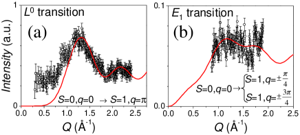
Figure 27: (Color online) $Q$ dependence of the integrated neutron scattering intensity of Cr₈ for the peak (a) $L^{0}$ and (b) $E_{1}$. Both peaks arise from transitions from the $S=0$ ground state into the $S=1$ sector, but the involved final spin multiplets differ by their shift quantum number $q$, as indicated in the panels. The solid lines represent the theoretical curves. Adapted from Waldmann et al., 2003.

Finally, also the $Q$ dependence of the peak intensities were analyzed. The experimental results for the $L^{0}$ and $E_{1}$ transitions and the theoretical expectations are presented in Fig. 27. The good agreement is obvious. However, most important, the $Q$ dependence provides a fingerprint of the underlying many-body structures of the quantum states involved in a transition. Hence, the observed different $Q$ dependencies of the $L^{0}$ and $E_{1}$ transitions directly demonstrate the different physical nature of the excitations in the $L$ band (rotations of the Néel vector) and the $E$ band (spin waves).

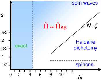
Figure 28: (Color online) Physical properties of the antiferromagnetic Heisenberg ring as a function of its size $N$ and the spin length $s$. In the blue shaded area quantum fluctuation are weak and the spin structure is essentially ”classical”. Here the $L\&E$-band concept becomes valid and $\hat{\bf H}_{AB}$ a good effective spin Hamiltonian. This ”classical” regime is reached when the size $N$ is significantly smaller than a characteristic correlation length $\xi$, which roughly increases exponentially with $s$. Adapted from Waldmann, 2002b.

Having demonstrated the $L\&E$-band picture for Cr₈, the question arises of how general it is. A conclusive answer is not yet available, but the results so far suggest Fig. 28: The $L\&E$ band concept works the better the larger $s$ and the smaller $N$ Engelhardt et al. (2006); Waldmann (2002b). The crossover is qualitatively determined by comparing the size $N$ of the cluster to a length $\xi$ characterizing the decay of the antiferromagnetic correlations with distance, as indicated in Fig. 28. A precise definition of $\xi$ can be subtle Haldane (1983a); Affleck et al. (1987), but in any (disordered) system the correlations decay on a characteristic length scale, which is what is meant by $\xi$. The spin length enters then through the dependence of $\xi$ on $s$, which, motivated by Haldane’s and other results Haldane (1983a, b); Affleck et al. (1987), is roughly exponential. Since for $s=1/2$, $\xi$ is about 6 sites, it is concluded that large $s=1/2$ clusters are distinguished from those with $s>1/2$ in that the $L\&E$ band picture is never obeyed in them.

The $L\&E$-band concept has some useful consequences, valid not only for the AFMHR. First, the $L$ band can well be reproduced by an effective Hamiltonian which may be constructed along the lines outlined in Sec. IV.2.3. This is carried out now for the example of the even antiferromagnetic wheels. Their lattice is bipartite and introducing two sublattices $A$ and $B$ is natural, where the spins on each sublattice are ferromagnetically aligned. Then an effective Hamiltonian is obtained by combining the spins on each sublattice to $\hat{\bf S}_{A}=\sum_{i\in A}\hat{\bf s}_{i}$ and $\hat{\bf S}_{B}=\sum_{i\in B}\hat{\bf s}_{i}$, and inserting $\hat{\bf s}_{i}=(2/N)\hat{\bf S}_{A}$ or $\hat{\bf s}_{i}=(2/N)\hat{\bf S}_{B}$, depending on the spin’s sublattice, into the microscopic Hamiltonian, which results in

$$\hat{H}_{AB}=-2j\hat{\bf S}_{A}\cdot\hat{\bf S}_{B},$$ (81)

with $j=a_{1}J$. For $a_{1}$ one finds $a_{1}=a_{1}^{AB}$, where $a_{1}^{AB}\equiv 4/N$. The two-sublattice Hamiltonian $\hat{H}_{AB}$ produces obviously an energy spectrum according to Eq. 79, immediately explaining the step-like magnetization curves (Fig. 22) and $L$ band in the energy spectrum. The approximation can be improved to yield nearly exact results if $a_{1}$ is slightly corrected to account for the weak quantum fluctuations Waldmann (2002a). For Cr₈ one obtains $a_{1}=a_{1}^{qm}$ with $a_{1}^{qm}=0.5586$.

Secondly, the nature of the $E$ band suggests applying SWT to the calculation of its energies. This route was explored in the last years, but the status is not yet clear and more work is needed. However, it seems that despite the conceptual problems of antiferromagnetic SWT the standard interacting SWTs do, at least for bipartite lattices, produce reasonable results for the energies of the $E$-band states in the $S=1$ sector. For instance, for the AFMHR the ”dispersion relation” $\epsilon(q)$ in Eq. (80) are obtained (vide infra).

IV.3.2 Antiferromagnetic wheels with ”intermediate” anisotropy

In antiferromagnetic wheels with substantial magnetic anisotropy the ground state and lowest excitation may better be described by quantum tunneling of the Néel vector (Sec. IV.3.3), but for the next-higher lying levels the $L\&E$-band picture is still appropriate, though $S$ mixing occurs as a novel feature. In the following the effects of a significant anisotropy on the excitations will be discussed by the example of CsFe₈, as it is one of the best characterized large magnetic clusters and the generic Hamiltonian Eq. (78) has been confirmed with high precision.

The chemical formula of CsFe₈ is Cs[Fe₈tea₈]Cl. Eight Fe³⁺ ions ($s=5/2$) form an almost perfect octagon with a Cs⁺ ion at the center (Fig. 21). Depending on the synthesis, the system co-crystallizes with different solvent molecules in space groups P4/n, Pna21, and P21/n Saalfrank et al. (1997), and the molecule exhibits ideal or approximate C₄ symmetry, but a dependence of the magnetic excitations on the solvent was experimentally not observed. CsFe₈ is a member of a family of wheels which are distinguished by the templating central alkaline ion, and a magneto-structural correlation was established Waldmann et al. (2001); Pilawa et al. (2003). The magnetic excitations in CsFe₈ were studied by low-temperature high-field torque magnetometry, single-crystal high-frequency EPR at Q-band and 190 GHz, single-crystal nuclear magnetic resonance (NMR) Schnelzer et al. (2007), and several INS experiments covering energies up to 25 meV Waldmann et al. (2001); Dreiser et al. (2010a); Schnelzer et al. (2007); Waldmann et al. (2005); Waldmann et al. (2006b); Dreiser et al. (2010b).

The data analysis could be accomplished by solving the microscopic Hamiltonian Eq. (78) using the numerical sparse matrix techniques described in Sec. IV.2.2. However, the Hilbert space dimension is 1 679 616 and the task can become time consuming. Hence, approximate schemes are desired, with the advantage that their accuracy can always be checked by comparing with the exact results from Eq. (78) for some few cases. The lowest-level description built on the strong-exchange limit works well for, e.g., EPR experiments, but involves many parameters and furthermore misses important effects (for a detailed description of the strong-exchange limit approach we refer to the book by Bencini and Gatteschi, 1990, or to Dreiser et al., 2010a). However, if only the energy levels in the $L$-band sector - to use the language of the previous section - are desired, a high-accuracy higher-level description is provided by the sublattice Hamiltonian approach. Applying the ideas used for the HDVV term (Sec. IV.3.1) to the anisotropy (and Zeeman) term in the microscopic Hamiltonian yields the sublattice Hamiltonian

$$\hat{H}_{AB}=-2j\hat{\bf S}_{A}\cdot\hat{\bf S}_{B}+d\left(\hat{S}^{2}_{A,z}+\hat{S}^{2}_{B,z}\right)+g\mu_{B}\hat{\bf S}\cdot{\bf B},$$ (82)

with $j=a_{1}J$ and $d=b_{1}D$, where $a_{1}=a_{1}^{AB}$ and $b_{1}=b_{1}^{AB}$ [$b_{1}^{AB}\equiv(2s-1)/(Ns-1)$]. The approximation can again be improved by adjusting $a_{1}$ and $b_{1}$ to account for the weak quantum fluctuations, which results in essentially exact energies and yields transition intensities to within 10% accuracy Waldmann (2002a); Waldmann et al. (2006b). For CsFe₈, $a_{1}^{qm}=0.5536$ and $b_{1}^{qm}=0.1870$. The energy spectrum of CsFe₈ is nearly identical to that of Cr₈ shown in Fig. 25, and the labeling of states and transitions are carried over.

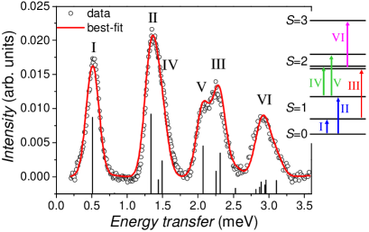
Figure 29: (Color online) Neutron-energy loss spectrum in CsFe₈, after background correction, at $T=17$ K, and best-fit curve calculated from Eq. (82). Adapted from Waldmann et al., 2006b.

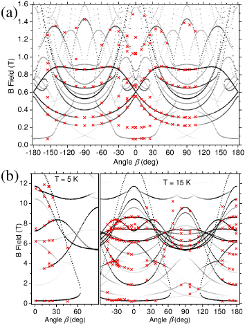
Figure 30: (Color online) Experimental (crosses) and simulated (doted lines) EPR transitions as observed in angle-resolved EPR experiments on single-crystals of CsFe₈ at frequencies of (a) Q band (35 GHz) ($T=25$ K) and (b) 190 GHz ($T=5$ and 15 K). Adapted from Dreiser et al., 2010a.

INS experiments allowed the observation of all $L$-band states up to $S=5$ at an energy of 14.4 meV [transitions $L^{0}$-$L^{4}$ with respect to Fig. 25]. The data could very accurately be simulated, Fig. 29. Also, the EPR transitions observed in angle-resolved high-frequency EPR in the field range of 0 - 12 T could be described with high accuracy, Fig. 30. In the EPR experiments the $L$-band states up to $S=4$ were probed. In the fits to the data only two free parameters, $2J$ and $D$, were involved. The determined values are given in Table. 6 (INS #2 and HFEPR).

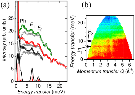
Figure 31: (Color online) Neutron-energy loss spectrum in CsFe₈ ($T=5$ K). (a) $Q$-sliced INS data, with curves offset for clarity. Gray curves represent the INS data recorded at $T=58$ K after Bose-correction. The solid line represents the best-fit simulation of the INS spectrum. (b) $S(Q,\omega)$ plot. Adapted from Dreiser et al., 2010b.

The excitation spectrum in CsFe₈ was also probed for energies up to 25 meV in a high-energy INS experiment Dreiser et al. (2010b). Results are shown in Fig. 31. At lower energies the transitions within the $L$ band are again observed, however, at energies of ca. 7.5 and 10 meV two further cold transitions are detected, which can unambiguously be related to the discrete spin-wave excitations $E_{1}$ and $E_{2}$ expected in an octa-nuclear antiferromagnetic wheel. Above transition $E_{2}$ no magnetic scattering intensity is observed, confirming the selection rule associated to the $L\&E$-band picture in Sec. IV.3.1. The determined $2J$ and $D$ values are listed in Table. 6 (INS #3).

The INS data were recorded on a non-deuterated poly-crystalline sample. This may explain the huge non-magnetic scattering in Fig. 31, which is typically observed in molecular nanomagnets above energies of ca. 2-3 meV. For CsFe₈ it could however very well be accounted for using a Bose-correction analysis (Sec. II.2.1), which allowed the unambiguous identification of the magnetic peaks, see Fig. 31(a).

Table 6: Comparison of the magnetic parameters for CsFe₈ obtained by different experimental techniques.

Technique	$2J$ [meV]	$D$ [meV]	Reference
torque	-1.90(10)	-0.045(3)	Waldmann et al.,2001
INS #1	-1.78(4)	-0.048(1)	Waldmann et al.,2005
INS #2	-1.80(2)	-0.050(1)	Waldmann et al.,2006b
INS #3	-1.79(5)	-0.050(7)	Dreiser et al.,2010b
HFEPR	-1.87(25)	-0.0493(1)	Dreiser et al.,2010a

Table 6 compiles the determined $2J$ and $D$ values, including those obtained by torque and high-resolution INS (INS #1) Waldmann et al. (2001, 2005). The consistency is excellent, in particular considering the large range of energy scales probed in the experiments ($\sim$0.01 meV in 35 GHz EPR, $\sim$10 meV in high-energy INS). Efforts were made to infer the significance of further terms in the microscopic spin Hamiltonian not included in Eq. (78). A $J_{1}-J_{2}$ modulation of the exchange constants along the wheel was found to be smaller than 20%, and the rhombic anisotropy to be negligible, $E=0.0000(3)$ meV Dreiser et al. (2010b, a).

The determined $2J$ value in the EPR experiment deserves a comment. The EPR selection rules do not allow a direct observation of exchange splittings (Sec. II.2.3). Exchange constants may though be determined indirectly, through the temperature dependence of the EPR resonance intensities, which however in large clusters is challenging, or through the $S$-mixing mechanism Liviotti et al. (2002); Waldmann and Güdel (2005); Wilson et al. (2006); Barra et al. (2007); Piligkos et al. (2009), which was the case in CsFe₈. In the strong-exchange limit, the anisotropy splitting produces the ”normal” zero-field splitting pattern, e.g., a $D$ term in the microscopic spin Hamiltonian produces a zero-field splitting of the spin multiplet, which follows the $M^{2}$ behavior corresponding to $\hat{S}^{2}_{z}$. However, if anisotropy is stronger, as compared to the exchange $J$, then the pattern is modified and deviations from $M^{2}$ occur. In perturbation theory this corresponds to higher-order terms $(\hat{S}^{2}_{z})^{n}$ with $n>1$ coming in, with weights $\propto(D/J)^{n}$. Detecting these shifts in the zero-field splitting pattern allows the indirect determination of the strength of the exchange. The excellent agreement of the EPR $2J$ value demonstrates hence that the generic Hamiltonian Eq. (78) does also describe the subtle $S$-mixing effects very well in CsFe₈.

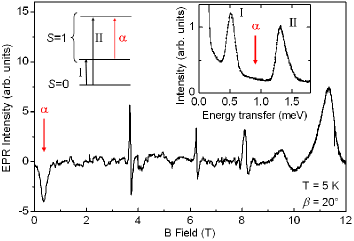
Figure 32: (Color online) 190 GHz EPR spectrum on a single crystal of CsFe₈. The intra-multiplet transition $\alpha$ is clearly observed. The inset to the left depicts the three lowest energy levels and the allowed INS transitions I, II, and $\alpha$. The inset to the right shows INS data recorded at $T=9.7$ K in which the transition $\alpha$ should have been observed if it were of appreciable intensity. Adapted from Dreiser et al., 2010a.

The comparison of the INS and EPR experiments reveal another interesting aspect of the excitations in antiferromagnetic wheels. According to the INS selection rules the transition $|S=1,M=0\rangle\leftrightarrow|S=1,M=\pm 1\rangle$, or $\alpha$ henceforth, is allowed and should be detected at appropriate temperatures, yet it is not observed in INS experiments, albeit in EPR experiments (Fig. 32). It turns out that intra-multiplet transitions, such as $\alpha$, are orders of magnitude weaker than inter-multiplet transitions because of the particular many-body structure of the wave functions, which is that of a bipartite lattice of two mesoscopically sized spins on each sublattice ($S_{A}=S_{B}=10$ in CsFe₈) Waldmann et al. (2005). By that reason the intra-multiplet transitions become too weak to be observed by INS. CsFe₈ provides a convincing example, since here the transition $\alpha$ should have easily been detected by INS, see Fig. 32. Hence, the combined INS and EPR data demonstrate directly a hallmark feature of antiferromagnetic wheels, namely the mesoscopic antiferromagnetic sublattice structure.

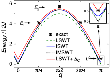
Figure 33: (Color online) Zero-temperature excitation spectrum of the $N=8$, $s=5/2$ AFMHR, as function of the shift quantum number $q$ as calculated using exact numerical diagonalization (stars) and the indicated SWTs (lines)(in the latter $q$ was assumed as continuous for clarity). LSWT = linear SWT, ISWT = interacting SWT, IMSWT = full-diagonalization interacting modified SWT, LSWT+$\Delta_{c}$ = linear SWT with a shift. Adapted from Dreiser et al., 2010b to which we also refer for details.

Although anisotropy is appreciable in CsFe₈, the energies of the spin-wave excitations $E_{1}$ and $E_{2}$ are actually little affected. This, and fundamental interest, motivated an analysis of the elementary excitations of the $N=8$, $s=5/2$ AFMHR model using different variants of SWT. All models provide predictions for the $E$-band states or the ”dispersion relation” $\epsilon(q)$ in Eq. (80), but only the last three yield also estimates for the singlet-triplet gap $\Delta$ ($=a_{1}|2J|$) or $L$-band indeed. The findings are compared in Fig. 33 to the exact energies. Interestingly, all SWT models reproduce roughly the spin-wave excitation spectrum, which supports the notion that the $L\&E$-band concept is essentially classical. However, significant differences exist, and the ISWT and LSWT+$\Delta_{c}$ models do best for the $E$-band excitations. As regards the singlet-triplet gap, the LMSWT and IMSWT estimate it almost a factor of two too small. LSWT+$\Delta_{c}$ comes closest, to within 7%. A similar analysis for the larger Fe₁₈ wheel ($N=18$, $s=5/2$) confirmed the observations Ummethum et al. (2012).

IV.3.3 Antiferromagnetic wheels with ”strong” anisotropy and quantum tunneling of the Néel vector

The possibility of quantum tunneling of the Néel vector (QTNV) in antiferromagnetic materials attracted huge interest Barbara and Chudnovsky (1990); Krive and Zaslavskii (1990); Gunther and Barbara (1995); Gider et al. (1995); Chudnovsky and Tejada (1998); Shpyrko et al. (2007), and initial attempts to establish QTNV concentrated on ferritin proteins Awschalom et al. (1992); Tejada (1996); Garg (1996); Gider et al. (1996). The prediction that coherent QTNV might also be realized in antiferromagnetic molecular wheels with strong anisotropy Chiolero and Loss (1998) stimulated intense research. In this context the molecules Fe₁₀ (Sec. IV.3), CsFe₈ (Sec. IV.3.2), and Fe₁₈ appeared as promising candidates (Fig. 21). Reviews and follow-up articles on the QTNV scenario in antiferromagnetic wheels are available Leuenberger et al. (2003); Meier and Loss (2001b); Konstantinidis et al. (2011).

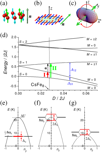
Figure 34: (Color online) (a,b) Classical ground-state spin configuration for a (a) $N=8$, (b) $N=18$ antiferromagnetic wheel with the Néel vector (long green arrow) pointing along (a) $\bf z$, (b) $\bf y$. (c) Shape of the potential $V({\bf n})$ in the case (B). The two tunneling paths from ${\bf n}=+y$ to $-y$ are indicated. Simulated low-lying energies of a $N=8$, $s=5/2$ antiferromagnetic wheel vs $D/(2J)$ in zero field ($M$ is then an exact quantum number). Transitions I and II are observed in INS experiments (Fig. 35). (e-g) Energy scheme as given by semiclassical theory for (e) Fe₁₈, (f) CsFe₈, and (g) Fe₁₀. Adapted from Konstantinidis et al., 2011; Waldmann et al., 2009, 2005.

The discussion in the following refers to Eq. (78). Due to the anisotropy the spin functions $|SM\rangle$ are mixed strongly and $S$ loses its significance as good quantum number. This changes also the dynamics of the Néel vector, defined as $\hat{\bf n}=(\hat{\bf S}_{A}-\hat{\bf S}_{B})/(S_{A}+S_{B})$, which is then not anymore that of a rotation but tunneling. In the quantum spectrum this may be seen by the fact that the two lowest levels (ground state & first excitation) approach each other but separate from the next higher-lying levels, as shown exemplarily in Fig. 34(d): $\Delta_{01}$ becomes smaller than e.g. $\Delta_{12}$.

A semi-classical theory provided a clear description Chiolero and Loss (1998); Meier and Loss (2001b). Depending on the magnetic parameters and strength and orientation of the magnetic field, several scenarios occur; we here focus on two: (A) $D<0$ and zero magnetic field and (B) $D>0$ and large magnetic fields with $\bf B$ along the $x$ axis. In both cases, the Néel vector is strongly localized along two directions, namely ${\bf n}=\pm{\bf z}$ (A) or $\pm{\bf y}$ (B). Classically, the ground state is then characterized by the spin configurations with Néel order sketched in Fig. 34(a) and (b), respectively, and rotation is hampered by an energy barrier, corresponding to a potential $V({\bf n})$ with minima at the respective orientations [Fig. 34(c)]. However, quantum fluctuations allow for tunneling of the Néel vector, which lifts the classical degeneracy and opens a tunneling gap $\Delta_{QTNV}$ in the energy spectrum, which then corresponds to $\Delta_{01}$.

The Néel-vector dynamics is characterized by the tunneling action $S_{0}/\hbar$, attempt frequency $\hbar\omega_{0}$, barrier height $\Delta U$, and tunneling amplitude $\Delta_{0}$,

$$S_{0}/\hbar = Ns\sqrt{2|D/(2J)|},$$ (83)

$$\hbar\omega_{0} = s\sqrt{8|D(2J)|},$$ (84)

$$\Delta U = Ns^{2}|D|,$$ (85)

$$\Delta_{0} = 8\hbar\omega_{0}\sqrt{\frac{S_{0}/\hbar}{2\pi}}\exp(-S_{0}/\hbar).$$ (86)

The two cases (A) and (B) need to be distinguished now, which we do through a parameter $c=2$ (A) and $c=1$ (B), respectively. The ground state energy is then given as $\frac{c}{2}\hbar\omega_{0}$, and the tunneling splitting as $c\Delta_{0}$ [in the case (A) the tunneling gap has to our knowledge not yet been calculated, but numerical results suggest $\Delta_{QTNV}\approx 2\Delta_{0}$]. The semi-classical theory for QTNV becomes valid for large tunneling actions $\frac{1}{2c}S_{0}/\hbar\gg 1$, which is equivalent to stating that the ground-state energy is smaller than the barrier height, $\Delta U\gg\frac{c}{2}\hbar\omega_{0}$, or the Néel vector strongly localized, $\langle 0|\hat{n}_{z/y}|1\rangle^{2}\rightarrow 1$, where the matrix element is given as $\langle 0|\hat{n}_{z/y}|1\rangle^{2}\approx 1-c/(S_{0}/\hbar)$, where $z$ (A) or $y$ (B) is the respective Néel vector component.

As regards applying the semi-classical theory some points are worth noticing. First, it turned out that the $J$ and $D$ values as they appear in Eq. (78) or through $a_{1}^{qm}$ and $b_{1}^{qm}$ in Eq. (82) should not be inserted in the semi-classical formulae, but ”corrected” $J$, $D$ values as they are obtained by using $a_{1}^{sc}\equiv 4/N$ and $b_{1}^{sc}\equiv 2Ns^{2}/[Ns(Ns+2)-3]$ Waldmann et al. (2009) (for a detailed discussion see Konstantinidis et al., 2011). Not doing so leads to e.g. significantly overestimated tunneling actions, which went unfortunately unnoticed in early works. Furthermore, the crossover from weak to strong anisotropy, or from rotation to tunneling of the Néel vector, is continuous and not abrupt [Fig. 34(d)], and the QTNV scenario is hence necessarily approximate Santini et al. (2005). This introduces some ambiguity, and different criteria for when QTNV is realized can be given, e.g., that the tunneling levels should fall below the top of the barrier or that the tunneling splitting should be exponentially small. It is noted in passing that since the semi-classical theory as it stands is an approximate theory, agreement with semi-classical theory is a sufficient but not necessary criterium for QTNV.

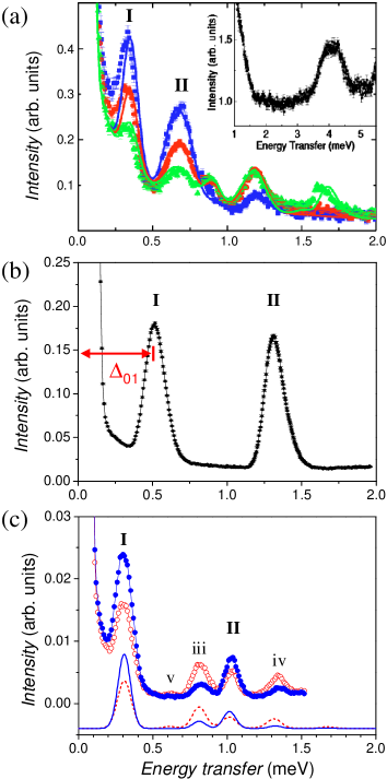
Figure 35: (Color online) Neutron-energy loss spectra for (a) Fe₁₀ [$T=$ 2 K (blue), 5 K (red), 10 K (green)], (b) CsFe₈ ($T=2.4$ K), and (c) Fe₁₈ [$T=$ 1.9 K (blue), 4.2 K (red)] showing transition I, which in the QTNV regime correspond to the Néel vector tunneling splitting $\Delta_{01}$. Adapted from Santini et al., 2005; Waldmann et al., 2005, 2009.

The low-lying excitations in zero field were measured by INS for Fe₁₀, CsFe₈, and Fe₁₈ Waldmann et al. (2005); Santini et al. (2005); Waldmann et al. (2009). Fe₁₀ and CsFe₈ were described before. The chemical formula of Fe₁₈ is [Fe₁₈(pd)₁₂(pdH)₁₂(O₂CEt)₆(NO₃)₆](NO₃)₆$\cdot$$x$MeCN ($x\approx 48$); the eighteen Fe³⁺ ($s=5/2$) ions are arranged in a cycle (Fig. 21) King et al. (2006). The system crystallizes in space group R3- and the molecule exhibits crystallographic S₆ symmetry. One nitrate and ca. 8MeCN solvent molecules are disordered. INS data for the three wheels are shown in Fig. 35. The lowest excitation I could clearly be detected as well as several higher excitations (for CsFe₈ see Sec. IV.3.2), which facilitated a precise determination of the magnetic parameters. In Fe₁₀ a substantial rhombic term $|E/D|=0.21$ was found, and structural disorder had to be included in the analysis. In Fe₁₈ a high-energy INS experiment evidenced a modulation of the exchange constants along the ring consistent with the C₃ symmetry Ummethum et al. (2012). Notably, the ratio of the excitation energies of transitions I and II decreases in the sequence of Fe₁₀, CsFe₈, and Fe₁₈. For better comparison of the wheels, the magnetic parameters reported in the original works were converted to $2j$ and $d$ of $\hat{H}_{AB}$, Eq. (82) (in case of Fe₁₀ the rhombic contribution was neglected and for Fe₁₈ the appropriate averaged $J$ was used). The results are listed in Table 7.

Table 7: Experimental values and characteristic parameters of QTNV for Fe₁₈ ($c=1$), CsFe₈ ($c=2$), and Fe₁₀ ($c=2$). Adapted from Konstantinidis et al. (2011).

	Fe18	CsFe8	Fe10
$2j$ [K]	-5.1	-11.1	-6.31
$d$ [K]	0.021	-0.104	-0.0276
$\Delta_{01}$ [K]	not measured	5.92	3.83
$S_{0}/\hbar$	5.90	4.03	3.42
$\Delta U$ [K]	22.2	22.5	9.25
$\frac{c}{2}\hbar\omega_{0}$ [K]	7.52	22.3	10.8
$c\Delta_{0}$ [K]	0.320	5.08	4.18
$(S_{0}/\hbar)/c$	2.95	1.01	0.96
$\langle 0|\hat{n}_{z/y}|1\rangle^{2}$	0.83	0.50	0.42
$\Delta_{QTNV}/\Delta U$	0.014	$\approx 0.23$	$\approx 0.45$

For both CsFe₈ and Fe₁₀ one finds $d<0$ or $D<0$, while for Fe₁₈ $D>0$. Hence, in CsFe₈ and Fe₁₀ [case (A)] the transition I observed by INS would directly correspond to the Néel vector tunneling gap if QTNV were realized in them. The tunneling gaps estimated by the semi-classical theory roughly agree with the observed gaps, but the other parameters compiled in Table 7 indicate that QTNV is not well realized in Fe₁₀, and that CsFe₈ is borderline. For $D>0$ as in Fe₁₈ QTNV does not occur at low fields Chiolero and Loss (1998), but in the high-field regime, which in Fe₁₈ is reached above 10.6 T [case (B)]. Here, QTNV is well realized in Fe₁₈ as e.g. indicated by the exponentially small tunneling gap. The situation in the three wheels is probably most clearly demonstrated by the energy diagrams shown in Fig. 34(e) - (g).

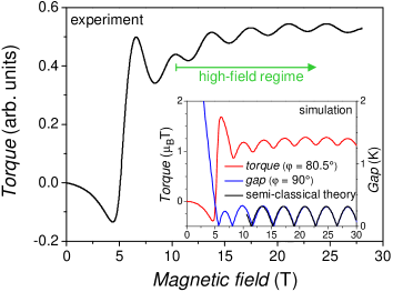
Figure 36: (Color online) Magnetic torque vs field for $B$ nearly perpendicular to $z$ (angle = 80.5^∘, $T=0.1$ K), showing ”wiggles” due to the oscillations of the Néel-vector tunneling gap. The inset shows the simulated field-dependent torque and the tunneling gap as calculated quantum mechanically and semiclassically. Adapted from Waldmann et al., 2009.

The high-field Néel vector tunneling gap in Fe₁₈ was not directly observed via spectroscopic techniques, but the field-dependent oscillations in the Néel vector tunneling gap due to quantum interference were detected in low-temperature high-field magnetic torque measurements Waldmann et al. (2009). In the semi-classical theory for case (B) the phase of the ground-state wave function contains a topological term $\pi Ng\mu_{B}B/|4(2J)|$, which is proportional to the field. Hence, in increasing fields the phase is repeatedly tuned through destructive and constructive interference, which gives rise to an oscillation of the tunneling splitting according to

$$\Delta(B)=\Delta_{QTNV}\left|\sin\left(\pi\frac{Ng\mu_{B}B}{4|2J|}\right)\right|.$$ (87)

Since the tunneling splitting also affects the ground-state energy, $E_{0}(B)=\epsilon(B)+\Delta(B)/2$, where $\epsilon(B)$ is a smooth function, the oscillations can be detected by magnetization or torque measurements at low temperatures. Indeed, the observed ”wiggles” in the torque curve (Fig. 36) do directly correspond to the oscillations in the tunneling gap, which is demonstrated e.g. by comparing the numerically calculated curves for the torque and the tunneling gap (inset to Fig. 36). The analysis also showed that the semi-classical theory yields highly accurate results, which underpins the notion of QTNV in Fe₁₈.

It is added that wiggles in the torque as function of field can also occur due to a first-order mixing of the $|S,M=-S\rangle$ and $|S+1,M=-S-1\rangle$ spin levels at the field-induced level-crossing points by the magnetic anisotropy; an example for this $S$-mixing mechanism will be presented below in Sec. IV.4.1. However, theoretically QTNV cannot be described by $S$-mixing of two spin levels reflecting its different underlying physics, and also experimentally, the two mechanisms can unambiguously be distinguished from each other. For instance, the dependence on the angle between magnetic field and anisotropy axis $z$ allows a clear-cut decision: In the $S$-mixing scenario the wiggles occur for both nearly parallel and perpendicular fields, in contrast to the observations in Fe₁₈, where ordinary staircase-like profiles are observed for parallel fields, as predicted by the QNVT scenario.

IV.4 ”Modified” antiferromagnetic molecular wheels

The ring topology considered in Sec. IV.3 can be varied in a number of ways, by ”slight” modifications. The topologies which will be addressed here can be put into four categories. First, one of the magnetic metal ions in the ring, which carry spin $s$, is replaced by another magnetic metal ion with different spin $s_{0}\neq s$. These clusters shall be denoted as ”doped wheels”, and the foreign $s_{0}$ ion as impurity. Second, the cyclic boundary conditions are changed to open boundaries, e.g., by replacing one of the magnetic ions in the ring with a diamagnetic ion or by removing one metal center. These clusters shall be denoted as ”short chains”. Third, a magnetic ion is added at the center of the ring with coupling paths such that the lattice remains bipartite. And fourth, a magnetic ion is added at the center with the coupling paths introducing spin frustration, then called ”discs”. Representative examples are Cr₇Ni, Cr₆, Mn-[3$\times$3], and a Fe₇ molecule, shown in Fig. 37.

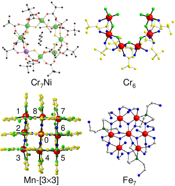
Figure 37: (Color online) Molecular structures of the doped wheel Cr₇Ni: [ⁿPr₂NH₂][Cr₇NiF₈Piv₁₆], short chain Cr₆: [R₂NH₂]₃[Cr₆F₁₁Piv₁₀(H₂O)], Mn-[3$\times$3] grid representing a wheel with magnetic center: [Mn₉(2POAP-2H)₆], and disc Fe₇: [Fe₇O₃tea₃Piv₉(H₂O)₃].

Much interest in such systems came from the theoretical suggestions that an uncompensated spin introduced into an antiferromagnetic wheel e.g. by doping may act as a tracer spin for the quantum tunneling of the Néel vector, which in this way could experimentally be observed and possibly manipulated by EPR methods, which otherwise would not be possible Meier and Loss (2001a); Meier and Loss (2001b). Furthermore, the excess spin may have $S^{\prime}=1/2$, which then suggests application of the cluster as quantum bit (qubit) Meier et al. (2003b, a); Troiani et al. (2005). Using such ”mesoscopic spin-1/2” clusters as ”spin cluster qubits” could provide advantages such as easier addressing. Significant progress in this direction have been made on the Cr₇Ni wheel, e.g., long coherence times were observed, magnetic coupling between two Cr₇Ni clusters introduced, and entanglement demonstrated Ardavan et al. (2007); Timco et al. (2009); Candini et al. (2010). Reviews are available Affronte et al. (2005, 2006). Since the physics is related mainly to the ground state, these exciting developments will however not be discussed. We will focus here on the basic question of the impact of topology on magnetic cluster excitations. The Mn-[3$\times$3] grid molecule will be considered first, followed by the doped wheels and short antiferromagnetic chains. An abundance of discs have been synthesized Hoshino et al. (2009a), but detailed studies of the cluster excitations were to our knowledge not reported.

IV.4.1 The Mn-[3$\times$3] grid molecule

Molecular [n$\times$m] grids attracted considerable interest in chemistry, for the employed preprogrammed self-assembly synthesis strategy and their physical properties. For reviews see Ruben et al., 2004; Dawe et al., 2009, the magnetic properties were reviewed in Waldmann, 2005a. The Mn-[3$\times$3] grid Zhao et al. (2000) is most interesting from the perspective of cluster excitations. The molecule may be crystallized with different counter ions and solvents, yielding e.g. [Mn₉(2POAP-2H)₆](ClO₄)₆$\cdot$3.75CH₃CN$\cdot$11H₂O (1) or [Mn₉(2POAP-2H)₆](NO₃)₆$\cdot$H₂O (2). Nine Mn²⁺ ($s=5/2$) metal ions are arranged on the vertices of a 3$\times$3 grid (Fig. 37). They crystalize in space group C2/c, and the molecules exhibit a slightly distorted D_2d symmetry with the S₄ symmetry axis (= $z$ axis) perpendicular to the grid plane. Considering the symmetry, the appropriate spin Hamiltonian for describing the magnetism reads

$$\hat{H} = -2J_{R}\left(\sum_{i=1}^{7}\hat{\bf s}_{i}\cdot\hat{\bf s}_{i+1}+\hat{\bf s}_{8}\cdot\hat{\bf s}_{1}\right)$$ (88)

$$-2J_{C}\left(\hat{\bf s}_{2}+\hat{\bf s}_{4}+\hat{\bf s}_{6}+\hat{\bf s}_{8}\right)\cdot\hat{\bf s}_{0}$$

$$+D_{R}\sum_{i=1}^{8}\hat{s}^{2}_{i,z}+D_{C}\hat{s}^{2}_{0,z}+g\mu_{B}\hat{\bf S}\cdot{\bf B},$$

where the spins are numbered as given in Fig. 37(c). In principle, the $D$ values for the corner and edge Mn ions could be different, but this was found to not affect the magnetism significantly.

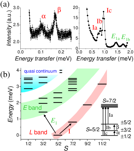
Figure 38: (Color online) (a) Neutron-energy loss spectra of Mn[3$\times$3] (2) at 2.5 K in two different energy ranges. (b) Simulated energy spectrum with anisotropy neglected. The observed INS transitions are indicated by arrows. The inset sketches the observed transitions within the $S=5/2$ ground and first excited $S=7/2$ multiplet. Adapted from Guidi et al., 2004.

From magnetization measurements, antiferromagnetic exchange interactions and a $S=5/2$ ground state were inferred, which can be rationalized by the classical spin configuration, where corner and central spins point up and edge spins point down. The excitation spectrum up to energies of 4 meV was studied by INS Guidi et al. (2004). Some results are presented in Fig. 38(a). The dimension of the Hilbert space is 10 077 696, and sophisticated numerical approaches had to be developed for analyzing the data. Good agrement was obtained for $2J_{R}=2J_{C}=-0.43$ meV and $D_{R}=D_{C}=-0.012$ meV. The higher-lying excitations revealed a small deviation of the exchange constants from the S₄ symmetry assumed in Eq. (88). The calculated energy spectrum with $D_{R}$ and $D_{C}$ set to zero is presented in Fig. 38(b). The two lowest transitions $\alpha$ and $\beta$ stem from the zero-field splitting of the $S=5/2$ ground state, as sketched in Fig. 38(b). Peaks Ia, Ib, and Ic correspond to transitions from the zero-field splitting levels of the ground multiplet to the next higher-lying $S=7/2$ multiplet, and peaks $E_{1a}$ and $E_{1b}$ go from the ground multiplet to the lowest $S=3/2$ multiplets.

Besides that the INS data of such a large cluster as Mn-[3$\times$3] were successfully interpreted, the inspection of the determined energy spectrum is interesting: As in antiferromagnetic wheels, the excitations may be classified as $L$ and $E$ band, or Néel-vector rotation and spin waves. This observation can be linked to the bipartite topology of the grid lattice, suggesting a ”classical” spin structure.

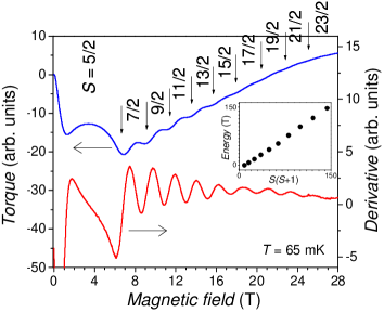
Figure 39: (Color online) Magnetic torque vs field (upper curve) and the field derivative (lower curve) for Mn-[3$\times$3] (1) with $B$ nearly perpendicular to the magnetic $z$ axis (angle = 80.5^∘, $T=0.1$ K), showing the oscillatory torque behavior. The inset shows the energies of the spin multiplets as extracted from the level-crossing fields Waldmann et al. (2011).

The $L$ band has been demonstrated in magnetic torque measurements Waldmann et al. (2004). At very low temperatures the torque exhibits an oscillatory field dependence, Fig. 39, which can be related to a sequence of level crossings, where the ground state changes from $S=5/2$ to $S=7/2$, $7/2\rightarrow 9/2$, and so one, similar to the situation in the wheels sketched in Fig. 23. In the experiments all states of the $L$ band up to $S=23/2$ were observed, and the energies of the multiplets as determined from the level-crossing fields do indeed follow the Landé pattern $S(S+1)$, as displayed in the inset to Fig. 39. Hence, the $L$ band (or tower of states or quasi-degenerate joints states), which is the precursor to long-range Néel ordering in the infinite lattice Bernu et al. (1992) has been experimentally demonstrated for the square-lattice topology.

These findings suggest the construction of an effective spin Hamiltonian for antiferromagnetic 3$\times$3 grids. Applying the procedure used for the antiferromagnetic wheels to the eight metal ions on the periphery yields

$$\hat{H}_{ABC} = -2j_{R}\hat{\bf S}_{A}\cdot\hat{\bf S}_{B}-2J_{C}\hat{\bf s}_{0}\cdot\hat{\bf S}_{B}$$ (89)

$$+d_{R}\left(\hat{S}^{2}_{A,z}+\hat{S}^{2}_{B,z}\right)+D_{C}\hat{s}^{2}_{0,z}$$

$$+g\mu_{B}\hat{\bf S}\cdot{\bf B},$$

with the sublattices $A=\{1,3,5,7\}$ and $B=\{2,4,6,8\}$, and $j_{R}=0.526J_{R}$ and $d_{R}=0.197D_{R}$ for the Mn-[3$\times$3] grid. $\hat{H}_{ABC}$ was indeed demonstrated to produce highly accurate results, and was found crucial in the analysis of experimental data Datta et al. (2007); Waldmann et al. (2004); Waldmann (2005b).

The oscillations in the torque signal originate from an interesting quantum-mixing mechanism Carretta et al. (2003a); Waldmann et al. (2004). A magnetic anisotropy is generally expected to induce mixing of spin multiplets ($S$ mixing), which often may be treated perturbatively, implying a ”small” effect (but see also Sec. IV.3.3). However, if two states are close in energy, i.e., essentially degenerate, then standard (non-degenerate) perturbation theory will obviously break down, and the effect of the perturbation not be small or mixing of the states large. The anisotropy produces thus a strong mixing of the $|S,M=-S\rangle$ and $|S+1,M=-S-1\rangle$ states involved at a level crossing, and the ground state is described as a superposition

$$|g\rangle\propto a(B)|S\rangle+b(B)|S+1\rangle$$ (90)

where the field-dependent $a$ and $b$ become equal at the level crossing (an obvious shorthand notation for the states was used; $a^{2}+b^{2}=1$). Since states with different total spin are mixed, the total spin will fluctuate strongly, also called quantum oscillations of the total spin Carretta et al. (2003a). This mixing is directly related to the oscillatory torque curve observed in experiment, which hence provides evidence for this phenomenon.

$S$ mixing should in principle also enable a direct detection of exchange splittings through EPR experiments, since the EPR selection rule $\Delta S=0$ would not hold exactly. However, the mixing is usually not strong enough for such EPR transitions to gain sufficient intensity, but through this mechanism the $S=5/2\rightarrow S=7/2$ transition could directly be observed in Mn-[3$\times$3] as function of field in a multi-frequency single-crystal EPR experiment Datta et al. (2007).

IV.4.2 ”Doped” even-membered antiferromagnetic wheels

A series of octa-nuclear hetero-nuclear wheels of general chemical formula [H₂NR₂][Cr₇M’F₈Piv₁₆], or Cr₇M’ in short, with e.g. M’ = Cu²⁺, Ni²⁺, or Mn²⁺ were synthesized Larsen et al. (2003a); Laye et al. (2005); Affronte et al. (2007); Baker et al. (2011b), and their excitations studied by different techniques, among which were low-temperature torque magnetometry Carretta et al. (2005), high-frequency EPR Piligkos et al. (2009), and INS Caciuffo et al. (2005); Baker et al. (2011b). Also an analogous Fe₇Mn cluster was investigated using INS Guidi et al. (2007). As mentioned before, the molecule Cr₇Ni has attracted most interest, because of its potential use in quantum information, and is focused on here.

The synthesis strategy resulting in Cr₇Ni is extremely flexible, and potentially many derivatives of Cr₇Ni exist Affronte et al. (2007). The material used in INS experiments was of chemical formula [H₂N(C₂D₅)₂][Cr₇NiF₈(O₂(C₅D₉)₁₆] and crystallizes in space group $P$4, without solvent molecules in the crystal lattice. Seven Cr³⁺ ($s=3/2$) ions and one Ni²⁺ ($s_{0}=1$) ion form a ring as shown in Fig. 37. The material has two advantageous properties for INS; it can be deuterated to a large extent and large single crystals can be grown. The appropriate generic spin Hamiltonian reads

$$\hat{H} = -2J\sum_{i=1}^{6}\hat{\bf s}_{i}\cdot\hat{\bf s}_{i+1}-2J^{\prime}\left(\hat{\bf s}_{1}+\hat{\bf s}_{7}\right)\cdot\hat{\bf s}_{0}$$ (91)

$$+D\sum_{i=1}^{7}\hat{s}^{2}_{i,z}+D^{\prime}\hat{s}^{2}_{0,z}+g\mu_{B}\hat{\bf S}\cdot{\bf B},$$

where the spins $\hat{\bf s}_{1}$ to $\hat{\bf s}_{7}$ refer to the Cr³⁺ ions, and $\hat{\bf s}_{0}$ is the spin of the Ni²⁺ ion. In view of the molecular symmetry, also a rhombic term $\sum_{i}E_{i}(\hat{s}^{2}_{i,x}-\hat{s}^{2}_{i,y})$ is expected and was evidenced in EPR experiments Piligkos et al. (2009), but was not resolved in magnetic torque and INS experiments Caciuffo et al. (2005); Carretta et al. (2005).

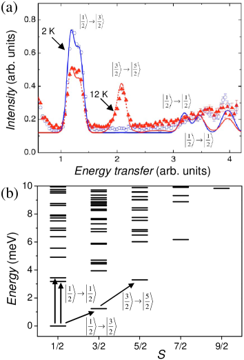
Figure 40: (Color online) (a) Neutron-energy loss spectra on Cr₇Ni at $T=2$ K and 12 K. Circles represent the experimental data; lines the simulation result. Adapted from Caciuffo et al., 2005. (b) Simulated energy spectra with anisotropy neglected. Observed INS transitions are indicated.

The exchange interactions in Cr₇Ni are antiferromagnetic and the ground state is $S=1/2$, consistent with the expectation from the classical spin configuration with Néel order. The magnetic excitations were studied by two INS experiments, which shall be described in the following. In a first experiment the excitations up to energies of $\sim$4 meV were detected Caciuffo et al. (2005). A spectrum is presented in Fig. 40(a). One large cold feature, with a double-peak structure, is observed at 1.27 meV, and a hot peak at 2.08 meV. At higher energies evidence for further magnetic scattering intensity is observed. The lowest feature can be associated to the transition from the $S=1/2$ ground state to the lowest-lying $S=3/2$ multiplet, and the double-peak structure of this feature to a zero-field splitting in the $S=3/2$ level. The zero-field splitting (0.15 meV) is much smaller than the center of gravity of the $S=3/2$ multiplet (1.27 meV); anisotropy is hence weak in this molecule, which is of relevance for its potential application as qubit Troiani et al. (2005). The 2.08 meV feature corresponds to an $S=3/2\rightarrow 5/2$ transition. The data could well be simulated using Eq. (91), yielding $2J=-1.46$ meV, $2J^{\prime}=-1.69$ meV, $D^{lig}=-0.03$ meV, and ${D^{lig}}^{\prime}=-0.6$ meV. The simulated energy spectrum with anisotropy neglected is shown in Fig. 40(b). The spectrum reveals again a $L$-band structure, which is confirmed by the INS experiment, and high-field torque magnetometry Carretta et al. (2005). Also $E$-band states are detected in the INS data.

The unique advantage of the Cr₇Ni system, that large deuterated single-crystals can be grown, allowed the direct experimental observation by INS of the level-crossing behavior as function of a magnetic field Carretta et al. (2007). In this experiment, a crystal of 0.4 g weight was measured at $T=66$ mK with magnetic field applied in a range of 0 - 11.5 T and an angle of $\theta=50^{\circ}$ with respect to the $z$ axis. Experimental results are shown in Fig. 41. At the level crossing at $B_{c}=10.5$ T a small gap of 0.12 meV is observed, i.e., an avoided level crossing, which originates from the $S$ mixing induced by the weak anisotropy effects. As explained in Sec. IV.4.1, at the level crossing where states become almost degenerate, the mixing effect will be strong, the wave function described by Eq. (90) with $|a|=|b|$, and the total spin oscillates. This INS experiment hence provides direct evidence for the quantum oscillations of the total spin in Cr₇Ni at the level crossing.

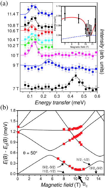
Figure 41: (Color online) (a) High-resolution neutron-energy loss spectra on a crystal sample of Cr₇Ni as function of magnetic field ($T=66$ mK, $\theta=50^{\circ}$). (b) Simulated low-lying energy levels as function of magnetic field (lines) with all observed INS transition energies included (squares). Adapted from Carretta et al., 2007.

IV.4.3 Short antiferromagnetic chains

The synthesis strategy which allowed us to generate the doped antiferromagnetic wheels in Sec. IV.4.2 also afforded the generation of short antiferromagnetic chains, either by replacing one magnetic metal ion in the ring-like structure by a diamagnetic ion such as Zn²⁺ or Cd²⁺, or modifying the synthesis method to yield structures called ”horseshoes” Affronte et al. (2007). The members of this family of clusters were studied, besides the thermodynamic techniques, by EPR Piligkos et al. (2007), XMCD Ghirri et al. (2009), NMR Amiri et al. (2010); Micotti et al. (2006), and INS Caciuffo et al. (2005); Baker et al. (2011a); Ochsenbein et al. (2007, 2008); Bianchi et al. (2009). Short antiferromagnetic chains were also obtained through doping the Fe₁₈ wheel (Sec. IV.3.3) with diamagnetic Ga³⁺ Henderson et al. (2008).

From the view point of the physics of the magnetic excitations, comparison of short antiferromagnetic chains with even-membered antiferromagnetic wheels, or chains with open and periodic boundary conditions, should prove interesting Ochsenbein et al. (2007), as well as comparing antiferromagnetic chains with even and odd number of metal centers Ochsenbein et al. (2008). A large body of literature exists on one-dimensional quantum spin chains, and also finite chains were studied Hagiwara et al. (1990); Di Tusa et al. (1994); Fujiwara et al. (1998); Bogani et al. (2004). It appears natural that the physical pictures developed there can also be extended to the short antiferromagnetic chains considered here. However, there are indications that this expectation is not fulfilled and the situation in the antiferromagnetic chains much more involved Konstantinidis et al. (2011). A definitive answer is not available at the moment. In the following we will describe the molecular horseshoe Cr₆, which represents a short antiferromagnetic chain with length $N=6$, exhibiting $S=0$ ground states.

The generic spin Hamiltonian for short antiferromagnetic chains is

$$\hat{H}=-2J\sum_{i=1}^{N-1}\hat{\bf s}_{i}\cdot\hat{\bf s}_{i+1}+D\sum_{i=1}^{N}\hat{s}^{2}_{i,z}+g\mu_{B}\hat{\bf S}\cdot{\bf B},$$ (92)

with $s_{i}=s$ for all ions. From molecular symmetry also a rhombic term $\sum_{i}E_{i}(\hat{s}^{2}_{i,x}-\hat{s}^{2}_{i,y})$ and a modulation of the exchange coupling constant, in particular at the ends of the chain, may be present. The presence of next-nearest-neighbor exchange was also suggested Bianchi et al. (2009). However, these effects are considerably smaller than those due to the leading terms given in Eq. (92).

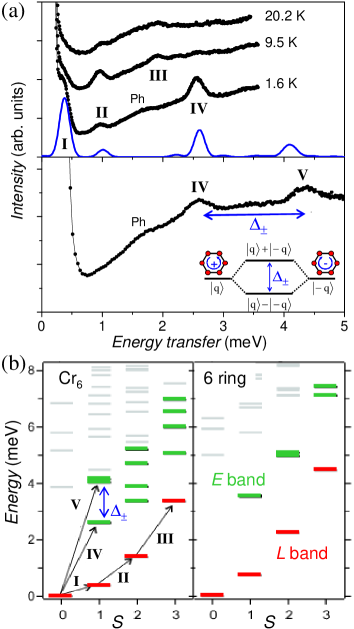
Figure 42: (Color online) (a) Neutron-energy loss spectra on Cr₆. The solid lines represent simulations). The inset sketches the formation of standing spin waves in a chain and the link to the gap in the spin-wave spectrum. (b) Simulated energy spectra for Cr₆ and a hypothetical $N=6$, $s=3/2$ antiferromagnetic wheel. The observed INS transitions and the gap in the $E$-band are indicated. Adapted from Ochsenbein et al., 2007.

Various derivatives of Cr₆ have been synthesized and studied by INS Larsen et al. (2003b); Baker et al. (2011a); Ochsenbein et al. (2007, 2008). Here the cluster [NH₂R]₃[Cr₆F₁₁Piv₁₀(H₂O)] is considered Larsen et al. (2003b). It crystallizes in space group $P$2₁/$c$, and the anion forms a string of six Cr³⁺ ($s=3/2$) ions, see Fig. 37. Using INS the magnetic excitation spectrum up to energies of 5 meV was studied Ochsenbein et al. (2007); results are shown in Fig. 42(a). Three cold feature I, IV and V are observed, and two hot transitions II and III. The data analysis yielded $2J=-1.27$ meV and $D=0$ in Eq. (92). The model was later refined to $2J=-1.4$ meV, $2J_{edge}=-1.1$ meV, $D=-0.028$ meV and $|E|=0.005$ meV, where $J_{edge}$ refers to the coupling strengths of the outer coupling paths Ochsenbein et al. (2008).

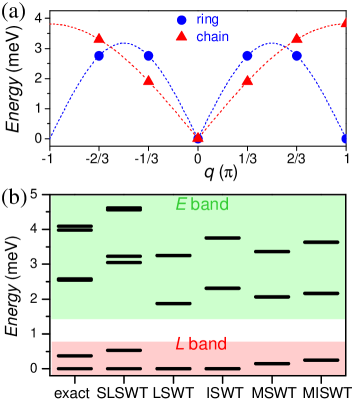
Figure 43: (Color online) (a) Spin-wave dispersion as obtained in linear SWT for Cr₆ and a hypothetical $N=6$, $s=3/2$ antiferromagnetic wheel. (b) Exact excitation energies in the $S=1$ sector of Cr₆ and comparison to the results of various variants of SWT. LSWT = linear SWT, ISWT = interacting SWT, MSWT = modified linear SWT, MISWT = modified interacting SWT, SLSWT = spin-level SWT. Adapted from Ochsenbein et al., 2007 to which we also refer for details.

In Fig. 42(b) are shown the simulated energy spectrum for Cr₆, using the parameters of the simplified model, and for comparison the energy spectrum of a hypothetical $s=3/2$ antiferromagnetic wheel. The $L\&E$-band picture is immediately recognized in Cr₆, and the observed INS transitions demonstrate the $L$- and $E$-band states. In comparison to the wheel, however, the $E$ band consists of two sub groups with an energy gap $\Delta_{\pm}$ in the $S=1$ sector. This splitting can be associated to the formation of standing spin waves in the chain, as opposed to running waves in the wheel. The basic argument is simple, and familiar from textbooks. In the hexa-nuclear wheel the spin waves with shift quantum number $q$ and $-q$, corresponding to left and right running waves, are degenerate because of cyclic symmetry. However, the open boundary in the chain or missing link acts as a perturbation lifting the degeneracy, resulting in the formation of the symmetric and anti-symmetric linear combinations of the wave function $|q\rangle$ and $|-q\rangle$, or standing waves indeed. The mechanism is sketched in Fig. 42(a). Hence the splitting of the $E$-band transitions into peaks IV and V observed in experiment directly demonstrates the standing spin waves in the Cr₆ antiferromagnetic chain.

These conclusions are supported by linear SWT Anderson (1952), which can approximate the energies of the $E$-band states in the $S=1$ sector Waldmann (2002b); Ochsenbein et al. (2007). The result for the Cr₆ horseshoe and the same hypothetical $N=6$, $s=3/2$ wheel as before is drawn in Fig. 43(a), clearly demonstrating the gap in the $E$-band spectrum because of the open-chain topology. This motivated an analysis of the exact quantum spectrum in Cr₆ by different variants of SWTs and a newly suggested spin-level SWT, which adds quantum-corrections to Eq. (81) in first-order Ochsenbein et al. (2007). Obviously interacting SWT does best in reproducing the exact energies, but the accuracy is a modest 8%. The results of a similar analysis for the CsFe₈ and Fe₁₈ antiferromagnetic wheels in Sec. IV.3.2 are recalled Dreiser et al. (2010b); Ummethum et al. (2012).

However, as mentioned before, the physics of the magnetic excitations in short antiferromagnetic chains, although displaying a $L\&E$-band structure in the energy spectrum, presents some subtleties which are difficult to understand Konstantinidis et al. (2011). In the eight membered short chain Cr₈Zn, for instance, a detailed analysis of the wave functions indicated a significant mixing of the $L$- and $E$-band states Bianchi et al. (2009).

IV.5 Spin frustration in antiferromagnetic molecular clusters

In the previous sections clusters with antiferromagnetic HDVV interactions on a bipartite lattice were discussed, but studying quantum spin-frustration effects in large clusters is obviously also of high interest. In fact, since the possible geometrical arrangements of metal ions and ligand linkages are not restricted by the constraint of translational invariance in ”zero-dimensional” clusters, competing interaction paths are almost always present in polynuclear magnetic molecules, and bipartite magnetic molecules are rather the exception than the rule. However, the research on the magnetic excitations in spin-frustrated systems concentrated on few model systems.

Regular antiferromagnetic spin triangles and lattices incorporating triangular units are most often considered in this context. The HDVV Hamiltonian of a triangle has been given in Eq. (61), where for a regular triangle $s_{i}=s$ for all ions and $J^{\prime}=J$. For $s=1/2$, the energy spectrum consists of a doublet of two $S=1/2$ spin multiplets in the ground state, which transforms according to the irrep $E$ of the $D_{3}$ symmetry group, and a higher-lying $S=3/2$ multiplet at energy $\frac{3}{2}|2J|$. The degeneracy of the two $S=1/2$ multiplets is (often) considered as criterium for spin frustration. However, small deviations such as distortions of the triangle leading to $J^{\prime}\neq J$ or Dzyaloshinski-Moriya interactions lift the degeneracy in the ground state opening a gap $\Delta$ (Fig. 44). The ratio $\Delta/|2J|$ may here be considered as a figure of merit.

This structure of low-lying energy levels has attracted huge interest for a variety of reasons. Spin frustration is one of them, but corresponding clusters are also attractive models for studying the Landau-Zener-Stückelberg (LZS) transitions or dissipation and decoherence in general Landau (1932); Zener (1932); Stückelberg (1932); Leggett et al. (1987); Dobrovitski et al. (2000); Chiorescu et al. (2000), or for applications as qubits Wernsdorfer et al. (2004), and Rabi oscillations were indeed observed Bertaina et al. (2008). Many molecular tri-nuclear clusters are available and were studied, also by INS, for their excitations. However, usually distortions are strong; the realization of regular triangles in bounded clusters is apparently not preferred by nature. The V₁₅ molecule is one of the best realizations of a regular triangle, according to its $\Delta/|2J|$, and its magnetic excitations are discussed in the next section.

Topologies with higher nuclearity, which also incorporate triangular units and are of high symmetry, such as the cubeoctahedron or icosidodecahedron, have also been intensely studied, however, mostly by theory Cépas and Ziman (2005); Schröder et al. (2005c); Rousochatzakis et al. (2008); Konstantinidis (2009); Schnack (2010). Only few experimental spectroscopic investigations of the cluster excitations are available. We will here focus on the magnetic Keplerate molecule Fe₃₀, which has become a main representative in this field of research, also because of its relationship to the Kagomé lattice (”Kagomé on a sphere”) Schnack (2010); Schnack et al. (2001); Rousochatzakis et al. (2008).

Many more molecules such as tetra-nuclear ”butterfly” and hepta-nuclear disc-like molecules or odd-membered antiferromagnetic wheels and cycles have been synthesized and studied for spin frustration effects.

IV.5.1 The V₁₅ molecule

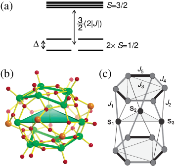
Figure 44: (Color online) (a) Sketch of the energy level scheme of an antiferromagnetic spin-1/2 triangle. (b) Structure of the anion of V₁₅. The thick green lines indicate the two hexagons, and the triangular area the spin triangle. (c) Sketch of the exchange interactions in the V₁₅ molecule. Adapted from Tarantul et al., 2007 and Chaboussant et al., 2004a.

The cluster [V₁₅As₆O₄₂(H₂0)]K₆$\cdot$8H₂O, or V₁₅ in short, contains 15 V⁴⁺ ions ($s=1/2$) whose arrangement can be described as two hexagons sandwiching a triangle, see Fig. 44(a) and (b) Müller and Döring (1988); Gatteschi et al. (1991). The system crystallizes in space group $R\bar{3}c$, and the molecule exhibits a nominal crystallographic $D_{3}$ symmetry, however, a water molecule sits at the center of V₁₅. Magnetic susceptibility demonstrated that the exchange interactions in V₁₅ indicated in Fig. 44(b) are antiferromagnetic and strong [$2J_{1}\approx 2J_{4}\approx-13$ meV, $2J_{2}\approx 2J_{3}\approx-26$ meV, $2J_{5}\approx-70$ meV], such that the hexagons are in a singlet state at temperatures below ca. 100 K and do not contribute magnetic moment. At low temperatures the magnetism can hence be described as that of a regular spin triangle with an effective antiferromagnetic interaction of $2J=-0.211(2)$ meV Chaboussant et al. (2002).

This picture was confirmed by detailed magnetization measurements at low temperatures Tarantul et al. (2007). However, a small gap in the $S=1/2$ ground-state doublet was detected. Magnetization data indicated $\Delta=7(2)$ $\mu$eV Barbara et al. (2002) and low-frequency EPR $\Delta=3$ $\mu$eV Kajiyoshia et al. (2007), while from INS a gap of $\Delta=35(2)$ $\mu$eV was concluded Chaboussant et al. (2002). The origin of the gap has been discussed controversially, most often it has been associated to Dzyaloshinski-Moriya interactions, but also to a distortion by e.g. the central water molecule.

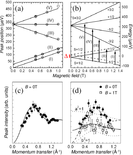
Figure 45: (a) Field dependence of the INS peak energies observed in V₁₅ at $T=45$ mK. Lines are fits to the data. (b) Derived energy spectrum and assignment of INS transitions. (c) $Q$ dependence of the intensities of peaks III + IV + V in zero field. (d) $Q$ dependence of the intensity of transitions III + IV + V at 0 T (circles) and transition I at 1 T (squares). Lines are fits to the data. Adapted from Chaboussant et al., 2004a.

Evidence for the latter came from an INS experiment performed on a fully deuterated polycrystalline sample of V₁₅ at ultra-low temperatures and with magnetic fields applied Chaboussant et al. (2004a). The field dependence of the observed INS peaks and their assignment are presented in Figs. 45(a) and (b), respectively, confirming spectroscopically the expected energy spectrum. The INS energies could excellently be fit and yielded $2J=-0.212(2)$ meV and $\Delta=27(3)$ $\mu$eV. A careful analysis of the magnetic field and $Q$ dependence of the INS peak intensities, shown in Figs. 45(c) and (d), allowed discriminating between Dzyaloshinski-Moriya interactions and distortions. It has been concluded that the gap $\Delta$ comes from a slightly distorted triangle, with exchange interactions $2J_{12}=-0.21$ meV, $2J_{23}=-0.23$ meV, and $2J_{13}=-0.20$ meV.

IV.5.2 The Fe₃₀ Keplerate molecule

The Fe₃₀ molecule [Mo₇₂Fe₃₀O₂₅₂(Mo₂O₇(H₂O))₂-(Mo₂O₈H₂(H₂O))(CH₃COO)₁₂(H₂O)₉₁]$\cdot$150H₂O consists of 30 antiferromagnetically coupled Fe³⁺ ions ($s=5/2$) which are located at the vertices of an icosidodecahedron Müller et al. (1999). The molecular structure is displayed in Fig. 46(a) and the iron metal core in Fig. 46(b). The spin arrangement clearly supports pronounced quantum-spin frustration effects, however, the large $s=5/2$ spins also suggest classical or semi-classical approaches Müller et al. (2001b). The dimension of the Hilbert space in this molecule is a staggering 2.2$\times$10²³ and understanding its magnetic excitation spectrum is obviously challenging. Fe₃₀ has in fact become an ideal test ground for developing theoretical schemes and physical concepts.

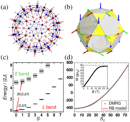
Figure 46: (Color online) (a) Molecular structure of Fe₃₀. (b) Fe³⁺ core forming an icosidodecahedron. The spin orientations in the classical ground state are represented by the arrows, the colors red, green and blue refer to the sublattices $A$, $B$, and $C$, respectively. (c) Low-lying energy spectrum as function of total spin $S$ as predicted in the rotational-band model Eq. (93), showing the $L$ and $E$ band. (d) Lowest energy in each sector $S_{z}$ as calculated by DMRG (black squares) and comparison to the $L$ band in the rotational-band model (red line). Both curves essentially superimpose confirming the $S(S+1)$ energy dependence of the lowest eigenstates in Fe₃₀. The inset shows the experimental magnetization curve. Pictures: (a,b,d) courtesy of J. Schnack, (c) adapted from Garlea et al., 2006.

Classically, the antiferromagnetic ground state is characterized by three sublattices $A$, $B$, and $C$, and is highly degenerate Axenovich and Luban (2001). Figure 46(b) depicts one of the possible classical ground-state spin configurations. For the quantum spectrum a rotational-band model with a three sublattice structure was conjectured Schnack et al. (2001), and based on ideas as those in Sec. IV.2.3 a Hamiltonian was derived,

$$\hat{H}_{ABC}=-\frac{2J}{5}\left(\hat{\bf S}_{A}\cdot\hat{\bf S}_{B}+\hat{\bf S}_{B}\cdot\hat{\bf S}_{C}+\hat{\bf S}_{C}\cdot\hat{\bf S}_{A}\right),$$ (93)

where $\hat{\bf S}_{A}$, $\hat{\bf S}_{B}$, $\hat{\bf S}_{C}$ describe the three sublattices, with spin lengths $S_{A}=S_{B}=S_{C}=25$. The predicted low-lying energy spectrum is presented in Fig. 46(c), and shows an $L\&E$-band structure, similar as in the antiferromagnetic wheels (Sec. IV.3.1). However, the degeneracies and spatial symmetry labels are of course different. For the existence of the $L$-band in Fe₃₀ solid evidence came from the experimental magnetization curve, which increases linearly with magnetic field up to saturation at a critical field $B_{c}=17.7$ T consistent with a $S(S+1)$ energy dependence of the lowest states in each spin sector [inset to Fig. 46(d)]. From the critical field the interaction strength has be estimated to $2J=-0.134$ meV. The $L$ band was also produced in a density matrix renormalization group (DMRG) calculation, Fig. 46(d) Exler and Schnack (2003).

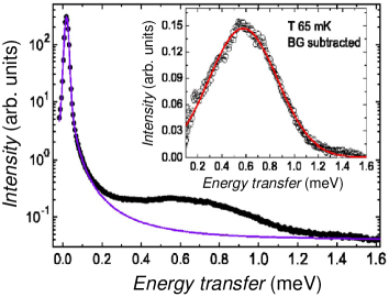
Figure 47: (Color online) Neutron-energy loss spectrum od Fe₃₀ at $T=65$ mK. The solid line represents the estimated background, and the such determined magnetic scattering is displayed in the inset. Adapted from Garlea et al., 2006.

The higher-lying magnetic excitations in Fe₃₀ were probed by INS experiments on a deuterated polycrystalline sample. An experimental spectrum is displayed in Fig. 47, showing a broad magnetic feature in the energy range 0.3-1.1 meV. The INS data could qualitatively be interpreted using Eq. (93) and associated to the $E$ band. Its excitation energy is predicted to $(26/5)|2J|=0.67$ meV [Fig. 46(c)] in rough agreement with the maximum in the neutron scattering intensity (inset to Fig. 47). The detailed analysis yielded $2J=-0.108$ meV. The width of the magnetic feature however remained unexplained.

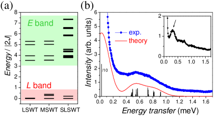
Figure 48: (Color online) (a) Low-temperature excitation spectrum of Fe₃₀ as predicted by linear SWT (LSWT), modified linear SWT (MSWT), and spin-level SWT (SLSWT). (b) Experimental INS spectrum of Fe₃₀ (points) and simulated spectrum using SLSWT (line). Inset: Experimental minus simulated spectrum, providing evidence for magnetic scattering at ca. 0.3 meV which the SLSWT model does not account for. Adapted from Waldmann, 2007.

In order to obtain a better insight the magnetic excitation spectrum was also calculated using modified linear SWT Cépas and Ziman (2005). The predicted spectrum is shown in Fig. 48(a). This theory suggests magnetic scattering in the energy range of $3.5|2J|$-$5.5|2J|$ and hence accounts at least partially for the observed broadening. A novel spin-level SWT, which implements a first-order quantum correction to Eq. (93), yielded an excitation spectrum in the range of $3.8|2J|-7.4|2J$ [Fig. 48(a)], and allowed to reproduce most of the observed magnetic scattering using $2J=-0.125$ meV [Fig. 48(b)], consistent to within 7% with the finding from the magnetic data Waldmann (2007). However, a peak-like magnetic scattering at ca. 0.3 meV is not reproduced.

It was pointed out that these SWT techniques, when applied to three- (and more) partite systems, have conceptual drawbacks Waldmann (2007). The spin-level SWT was later extended to higher-orders Schnalle et al. (2009), further emphasizing this point. A fully satisfying understanding of the magnetic excitations in Fe₃₀ is still lacking Garlea et al. (2006).

V Single-molecule magnets

V.1 Introduction

The single-molecule magnets (SMMs) are a special subclass of the molecular nanomagnets. Some prominent examples are shown in Fig. 49. The SMMs are distinguished by exhibiting slow relaxation of the magnetization or magnetic hysteresis at low temperatures, below a blocking temperature $T_{B}$. This phenomenon is not due to a long-range ordered magnetic ground state as in conventional magnets, but arises from an energy barrier for spin reversal at the molecular level. Furthermore, quantum phenomena such as quantum tunneling of the magnetization are observed as characteristic steps in the magnetic hysteresis curves. These unique magnetic properties discovered about 15 years ago stimulated enormous research and allowed addressing fundamental questions in quantum mechanics as well as suggested applications in information technology as classical or quantum bits or in molecular spintronics. Many authoritative reviews and books were written, some of them are Christou et al., 2000; Chudnovsky and Tejada, 1998; Gatteschi and Sessoli, 2003; Gatteschi et al., 2006b; Friedmann and Sarachik, 2010; Bogani and Wernsdorfer, 2008; del Barco et al., 2005; Barbara and Gunther, 1999; Leuenberger et al., 2003.

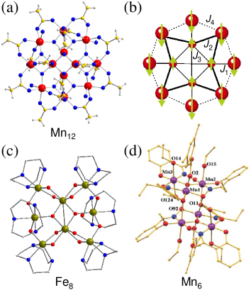
Figure 49: (Color online) Molecular structures of three prominent SMMs, (a) Mn₁₂: [Mn₁₂O₁₂(CH₃COO)₁₆(H₂O)₄], (c) Fe₈: [Fe₈O₂(OH)₁₂(tacn)₆]Br₈$\cdot$9H₂O, (d) Mn₆: [Mn₆O₂(Et-sao)₆(O₂CPh(Me)₂)₂(EtOH)₆]. Panel (b) shows the metal core in the Mn₁₂ molecule, the exchange coupling paths, and the classical ground state spin configuration.

The magnetic spectrum in the SMMs is in principle also described by the microscopic spin Hamiltonian Eq. (75). However, the most fascinating SMM phenomena such as quantum tunneling of the magnetization are related to the ground-state multiplet, and the anisotropy splittings in it. The effective spin Hamiltonian, which is known as ”rigid-spin” or ”giant-spin” or ”single-spin” model, reads then

$$\hat{H} = \hat{H}_{z}+\hat{H}_{\perp}$$ (95)

$$= D\hat{S}_{z}^{2}+B^{0}_{4}\hat{O}^{0}_{4}(S)$$

$$+E\left(\hat{S}_{x}^{2}-\hat{S}_{y}^{2}\right)+B^{2}_{4}\hat{O}^{2}_{4}(S)+B^{4}_{4}\hat{O}^{4}_{4}(S),$$

where $S$ is the total spin of the ground-state multiplet. The terms were distinguished into $\hat{H}_{z}$ and $\hat{H}_{\perp}$ according to whether they commute with $\hat{S}_{z}$ or not, and only the usually most relevant higher-order terms were listed [terms up to 6^th order were demonstrated in high-precision experiments Barra et al. (2007), compare also with Sec. III.3.5]. In a magnetic field the Zeeman terms $\mu_{B}g_{z}\hat{S}_{z}B_{z}$ and $\mu_{B}(g_{x}\hat{S}_{x}B_{x}+g_{y}\hat{S}_{y}B_{y})$ have to be added to $\hat{H}_{z}$ and $\hat{H}_{\perp}$, respectively. In principle the giant-spin model can be derived perturbatively from Eq. (75).

In a SMM the uniaxial anisotropy, which is the dominant zero-field splitting term in Eq. (95), has to be of easy-axis type or $D<0$. The energy levels $|M\rangle$ of the ground-state spin multiplet organize then into a parabolic band according to $DM^{2}$, with the $M=\pm S$ levels being lowest and separated by an energy barrier of height $U=|D|S^{2}$ for integer and $U=|D|(S^{2}-1/4)$ for half-integer $S$ (see inset to Fig 50). This energy barrier is responsible for the slow relaxation of the magnetization. The non-commuting terms contained in $\hat{H}_{\perp}$ induce a mixing between the $|M\rangle$ levels, or quantum tunneling indeed.

As regards spectroscopy, the major goal is the precise determination of the parameters in the giant-spin Hamiltonian, where in particular the non-commuting terms in $\hat{H}_{\perp}$ are of most interest, because of their relation to the quantum tunneling rates. As the relevant transitions are intra-multiplet with $\Delta S=0$ many experimental techniques can accomplish the task. EPR is one of them, and high-frequency high-field EPR has indeed played a most important role Gatteschi et al. (2006a). INS has also been very valuable, adding the advantage of a zero-field spectroscopy.

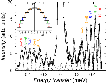
Figure 50: (Color online) INS spectrum of Fe₈ at 9.6 K. Circles represent the experimental data, dashed lines Gaussian fits, and the solid line a simulation. The transitions are labeled according to $|\pm M\rangle\rightarrow|\pm M^{\prime}\rangle$. The inset shows the parabolic energy spectrum with the allowed INS transitions indicated by arrows. Adapted from Caciuffo et al., 1998

Figure 50 shows an INS spectrum recorded on a non-deuterated sample of the compound [Fe₈O₂-(OH)₁₂(tacn)₆]Br₈$\cdot$9H₂O, or Fe₈ henceforth Caciuffo et al. (1998). The molecule contains eight Fe³⁺ ions ($s=5/2$) in a butterfly-like arrangement, Fig. 49(c). It crystallizes in space group P1 and exhibits approximate D₂ molecular symmetry Wieghardt et al. (1984). The frustrated AFM interactions in the molecule result in a $S=10$ ground state. In the experimental INS data in Fig. 50 the allowed $\Delta M=\pm 1$ transitions are observed, demonstrating the zero-field splitting in this spin multiplet. The ”picket-fence” INS spectrum, which is typical for SMMs, results from the fact that the transition energies given by the dominant $D$ term in Eq. (95) vary as $|D|(2M-1)$ or linearly in $M$. Slight deviations from the regular pattern are however seen, which relate to the other terms in Eq. (95), and precise values for its five parameters could be determined Caciuffo et al. (1998). Besides the scientific impact of this work, it also showed that excellent INS data can be recorded on non-deuterated samples of molecular nanomagnets, which established the basis for many of the subsequent INS works in this area.

Most of the SMMs which have been synthesized so far are based on 3d metal ions, and several of them were studied by INS, but mostly for the transitions within the ground-state multiplet (for reviews see Basler et al., 2003; Bircher et al., 2006). However, being related to anisotropy and not the exchange splittings, these studies shall not be further discussed here; Fe₈ may serve as a representative example. The potential of INS to also detect exchange splittings has been applied to only very few SMMs, such as Fe₄ Carretta et al. (2004b), Fe₈ Carretta et al. (2006), Mn₁₂, and Mn₆, and derivates of them. In the following the situation in Mn₁₂ and Mn₆ will be presented.

It is added that in the last few years the focus shifted from 3d-based SMMs to 3d-4f or 4f SMMs (also 5d ions became of interest). Since 4f ions are type J and bring in significant anisotropy, while exchange interactions are weak, the analysis of experimental data is typically more involved than in 3d-based type S/Q clusters. INS work on lanthanide containing SMMs has just begun Klokishner et al. (2009b); Dreiser et al. (2012), but promises exiting results in the future.

V.2 The Mn₁₂ cluster

The compound [Mn₁₂O₁₂(CH₃COO)₁₆(H₂O)₄], or Mn₁₂ in short, was the first molecule for which SMM behavior and quantum tunneling of the magnetization was observed below a blocking temperature of ca. 3.5 K Gatteschi et al. (2006b), and became the prototype SMM. The system crystallizes in space group $I_{4}$, and the molecule exhibits $S_{4}$ symmetry Lis (1980). It contains an inner tetrahedral core of four Mn⁴⁺ ions ($s=3/2$) and an outer ring of eight Mn³⁺ ions ($s=2$), Fig. 49(a). The nearest-neighbor Heisenberg exchange interactions in the cluster result in a total spin $S=10$ ground state, whose classical spin structure can be depicted as displayed in Fig. 49(b). The molecule’s properties in its $S=10$ ground-state multiplet have been heavily investigated Gatteschi et al. (2006b), also by INS Hennion et al. (1997); Mirebeau et al. (1999); Zhong et al. (1999); Bircher et al. (2004); Sieber et al. (2005); Waldmann et al. (2006a).

However, understanding how the competing Heisenberg interactions in the molecule give rise to the $S=10$ ground state is also of high interest, since through the $S$-mixing effects induced by the anisotropy the higher-lying spin multiplets can also significantly affect the $S=10$ ground-state multiplet and tunneling rates Carretta et al. (2004a); Barra et al. (2007). Several attempts were made to infer the values of the exchange constant $J_{1}$, $J_{2}$, $J_{3}$ and $J_{4}$ [see Fig. 49(b)] with controversial conclusions Sessoli et al. (1993); Hartmann-Boutron et al. (1996); Regnault et al. (2002); Raghu et al. (2001).

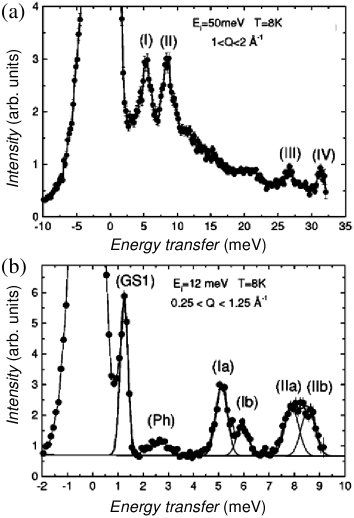
Figure 51: Neutron-energy loss spectra of Mn₁₂ recorded in two energy regimes. Data were recorded at the direct TOF spectrometer MARI at Rutherford Appleton Laboratory ISIS. Adapted from Chaboussant et al., 2004b.

The issue was targeted by high-energy INS experiments on a deuterated sample of Mn₁₂ Chaboussant et al. (2004b). INS spectra are shown in Fig. 51. A peak at ca. 1.2 meV is found, which originates from the $|\pm 10\rangle\rightarrow|\pm 9\rangle$ transition within the $S=10$ ground-state multiplet [$D=-0.057$ meV Bircher et al. (2004)]. Besides that, several inter-multiplet transitions reflecting the exchange splittings were observed in the energy range up 35 meV. From a detailed analysis of the experimental data the energy level scheme presented in Fig. 52 was derived. Interestingly, the anisotropy splittings in Mn₁₂ are not significantly smaller than the exchange splittings, as expected in the strong-exchange limit, which can be seen in Fig. 52(a) from the fact, that the lowest level of the lowest $S=9$ multiplet falls below the top of the $S=10$ ground-state multiplet. Hence, $S$ mixing plays a relevant role, which was later confirmed in a high-precision EPR experiment on the $S=10$ ground state Barra et al. (2007). Using numerical large-scale calculations, the exchange coupling constants were determined to $2J_{1}=-5.79$ meV, $2J_{2}=-5.33$ meV, $2J_{3}=-0.67$ meV and $2J_{4}=-0.48$ meV.

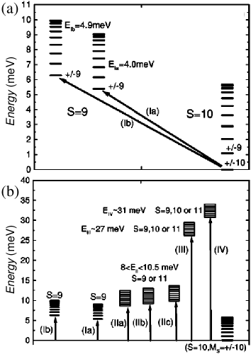
Figure 52: Energy level scheme as derived from the experimental INS data. Panel (a) shows a zoom into the low-energy spectrum. Adapted from Chaboussant et al., 2004b.

The exchange couplings $J_{3}$ and $J_{4}$ are one order of magnitude smaller than $J_{1}$ and $J_{2}$, and spin frustration is hence small in the Mn₁₂ molecule, which justifies the interpretation of the $S=10$ ground state in terms of the classical spin configuration shown in Fig. 49(b) and suggests a topological relation to AFM wheels Waldmann (2005a). In the context of Sec. IV.3.1, this implies that the $L\&E$-band concept is also realized in the Mn₁₂, which was underlined by a successful linear SWT analysis of the INS excitation spectrum Chaboussant et al. (2004b).

V.3 The Mn₆ clusters

The SMM [Mn₆O₂(Etsao)₆(O₂CPh(Me)₂)₂(EtOH)₆], or Mn₆ henceforth, which has been synthesized 14 years after the initial discovery of SMM behavior in Mn₁₂ Sessoli et al. (1993), was yet the first molecule found to exhibit a higher anisotropy barrier than that in Mn₁₂ Milios et al. (2007b). It contains six Mn³⁺ ions ($s=2$), which are arranged into two triangles linked by oxygen atoms, see Fig. 49(d). It crystallizes in space group P2₁/n and the molecule exhibits C_2h symmetry Milios et al. (2007b). Several derivates of this molecule have been synthesized and a magneto-structural correlation for the exchange couplings established Milios et al. (2007a).

Magnetic measurements demonstrated a $S=12$ ground state due to overall FM exchange interactions in the cluster. The zero-field splitting parameter in the $S=12$ ground state was estimated to $D\approx-0.054$ meV, corresponding to an energy barrier of $|D|S^{2}\approx 7.7$ meV. The exchange couplings were however determined to $2J\approx 0.4$ meV, hence suggesting that in Mn₆ $S$ mixing is very strong and the strong-exchange limit or giant-spin model break down.

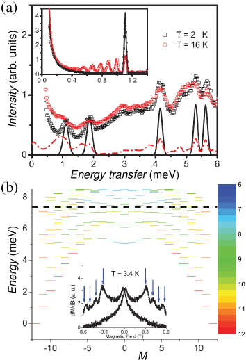
Figure 53: (Color online) (a) Neutron-energy loss spectra in Mn₆ recorded for two energy regimes up to 6 meV at the indicated temperatures (symbols). The lines represent simulations using Eq. (96) and the parameters given in the text. (b) Calculated energy spectrum as function of $M$. The color represents the value of the expectation value $\langle\hat{\bf S}^{2}\rangle$. Adapted from Carretta et al., 2008.

This has been indeed convincingly confirmed in an INS experiment on a non-deuterated sample of Mn₆ Carretta et al. (2008). Experimental INS data recorded in two energy windows are presented in Fig. 53(a). At low energies, at 1.1 meV and below, the ”picket-fence” spectrum characteristic for the transitions within the ground-state multiplet of a SMM is observed, see inset to Fig. 53(a). However, at already slightly higher energies (1.9 meV) the first inter-multiplet transition appear, followed by several more in the experimental energy range of 6 meV. This directly points to the fact, that several higher-lying spin multiplets are partially nested with the ground-state multiplet.

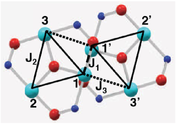
Figure 54: (Color online) The core of Mn₆ with the labeling of the Mn³⁺ sites and the assumed coupling paths indicated. Adapted from Carretta et al., 2008.

The data analysis was based on the Hamiltonian

$$\hat{H} = -2\sum_{i<j}J_{ij}\hat{\bf s}_{i}\cdot\hat{\bf s}_{j}+\sum_{i}\left[D_{i}\hat{s}_{iz}^{2}+B^{0}_{4i}\hat{O}^{0}_{4}(s_{i})\right],\quad$$ (96)

where three exchange coupling paths $J_{1}$, $J_{2}$, $J_{3}$ were assumed as displayed in Fig. 54. The ligand-field parameters for sites 1 and 1’, 2 and 2’, and 3 and 3’ are identical by symmetry, those of sites 2, 3, 2’, 3’ were assumed to be equal, and $B^{0}_{4,1}/B^{0}_{4,2}=D_{1}/D_{2}$ employed. The experimental data could be excellently reproduced with the best-fit parameters $2J_{1}=0.84(5)$ meV, $2J_{2}=0.59(3)$ meV, $2J_{3}=-0.01(1)$ meV, $D_{1}=-0.20(1)$ meV, $D_{2}=-0.76(2)$ meV, and $B^{0}_{4,1}=-0.0010(3)$ meV. The resulting simulated energy spectrum is shown in Fig. 53(b), which demonstrates that the energies of the $|M\rangle$ states of the $S=12$ ground-state multiplet do not follow the generic parabolic $M^{2}$ curve but deviate strongly from it at higher energies, and that indeed several higher-lying $S=11$ multiplets fall below the top of the $S=12$ multiplet. In Carretta et al., 2008 it was further demonstrated that this unique structure of the energy spectrum has significant effects on the magnetic relaxation rates.

VI Quantum spin systems

VI.1 Introduction

Quantum spin systems have been attracting much attention due to numerous magnetic features which cannot be interpreted by conventional spin models Sachdev (2008). In particular, classical magnetic phases such as ferromagnetism and Néel antiferromagnetism are prevented by (strong) quantum fluctuations, which are present in magnetic compounds if some of the following conditions are fulfilled:

(i) The spin quantum number of the magnetic ions is low, i.e., $s_{i}=1/2$ or 1.

(ii) The dimensionality of the magnetic system is low, i.e., $d=1$ or 2.

(iii) The connectivity of the network of magnetic ions (i.e., the number of spins to which each spin is coupled) is low.

(iv) The interactions between the magnetic ions are geometrically frustrated.

Representatives of the categories (i) and (ii) have been the subject of detailed investigations for a long time. They include one-dimensional magnets such as KCuF₃ Lake et al. (2005); Hutchings et al. (1979) and two-dimensional magnets such as La₂CuO₄ Headings et al. (2010); Coldea et al. (2001); Vaknin et al. (1987), the latter being of tremendous interest due to the observation of doping-induced superconductivity Bednorz and Müller (1986). More recently, novel materials have been synthesized which are formed by two and three magnetically coupled spin chains, e.g., two-leg spin ladders such as SrCu₂O₃ Azuma et al. (1994) and (C₅H₁₂N)₂CuBr₄ Rüegg et al. (2008); Thielemann et al. (2009) as well as three-leg spin ladders such as Sr₂Cu₃O₅ Azuma et al. (1994). Typical realizations of the category (iii) are weakly coupled dimer-based compounds including KCuCl₃ Kato et al. (1998); Cavadini et al. (1999), TlCuCl₃ Oosawa et al. (2002); Rüegg et al. (2003), NH₄CuCl₃ Kurniawan et al. (1999); Rüegg et al. (2004b), BaCuSi₂O₆ Jaime et al. (2004); Sebastian et al. (2005); Rüegg et al. (2007), SrCu₂(BO₃)₂ Kodama et al. (2002); Kageyama et al. (2000), Cs₃Cr₂Br₉ Leuenberger et al. (1985); Grenier et al. (2004), Sr₃Cr₂O₈ Quintero-Castro et al. (2010); Wang et al. (2011), and Ba₃Mn₂O₈ Uchida et al. (2002); Stone et al. (2008). Trimer-based compounds such as La₄Cu₃MoO₁₂ Qiu et al. (2005) as well as the compound SrCu₂(BO₃)₂ (characterized by an array of mutually perpendicular dimers) fulfill in addition the criterion (iv).

According to the topic of the present work, we will consider here only compounds for which the presence of magnetic clusters is the most important ingredient to understand their quantum spin properties. The following sections will therefore focus firstly on weakly interacting AFM dimer systems, for which quantum phase transitions involving gapless excitations and Bose-Einstein condensation have been observed most convincingly Giamarchi et al. (2008). Secondly, the phenomenon of a spin-Peierls transition will be described that occurs in quasi one-dimensional (1D) antiferromagnets due to the formation of spin pairs as a result of dimerization of the regular array of magnetic ions Bray et al. (1975). Thirdly, the formation of magnetic polarons observed in transition-metal perovskites will be discussed which evolve upon hole doping and behave like magnetic clusters embedded in a non-magnetic matrix Phelan et al. (2006).

VI.2 Dimer-based antiferromagnets

In dimer-based compounds the two magnetic ions are antiferromagnetically coupled according to the spin Hamiltonian Eq. (47). In contrast to isolated dimer systems discussed in Sec. III, the coupling between the dimers cannot be neglected, but the intra-dimer exchange coupling $J_{0}$ is larger than the coupling between the dimers $J_{1}=J_{0}/\gamma$. As long as $\gamma\gg 1$, the thermodynamic magnetic properties resemble those of isolated dimer systems, i.e., the dimer ground state $|S,M\rangle$ is a singlet $|0,0\rangle$, and so preserves full rotational invariance, unlike the Néel state of a square lattice antiferromagnet with $\gamma=1$. The singlet state is separated from the excited triplet states $|1,+1\rangle$, $|1,0\rangle$ and $|1,-1\rangle$ by an energy gap $\Delta=2|J_{0}|$. This picture is confirmed by the magnetic susceptibility measured for the dimer compound KCuCl₃ Tanaka et al. (1997) as shown in Fig. 55(a), which readily allows the determination of the gap energy, similar to the analysis of Fig. 2. However, the high-field magnetization data Oosawa et al. (2002) displayed in Fig. 55(b) are basically different from the case observed for isolated cluster systems. The latter exhibit sharp step-like enhancements of the magnetization (see Figs. 11 and 22), which are absent for KCuCl₃. Instead, the magnetization increases rather slowly above the critical field $B_{c}\approx 23$ T, and the saturation moment of 1 $\mu_{B}$/Cu²⁺ is reached at the saturation field $B_{s}\approx 53$ T far above $B_{c}$. This is due to the inter-dimer coupling $J_{1}$ giving rise to energy dispersion of the singlet-triplet excitations which may be called triplons. The triplon dispersion can be calculated in the random phase approximation Jensen and McIntosh (1991), since perturbation theory in $1/\gamma$ is well defined. For the case of dimers forming a square lattice we find

$$E_{M}({\bf k}) = -2J_{0}-2J_{1}\left[\cos(k_{x}d)+\cos(k_{y}d)\right]+g\mu_{B}BM,$$

where ${\bf k}=(k_{x},k_{y})$ is the quasiparticle wave vector, $d$ the lattice constant, $B$ an external magnetic field, and $M=0,\pm 1$. In zero field the three triplons are degenerate. With increasing field the triplons are split into three branches with $M=+1,0,-1$ as shown in Fig. 56(a). At a critical magnetic field $B_{c}$, the energy of the lowest triplet component $|1,+1\rangle$ intersects the ground-state singlet $|0,0\rangle$ and the ground state changes, thus $B_{c}$ is a quantum critical point separating a gapped spin-liquid state ($B<B_{c}$) from a field-induced magnetically ordered state ($B>B_{c}$). The triplet components $|1,+1\rangle$ can be regarded as bosons with hard-core repulsion, thus Bose-Einstein condensation occurs at the quantum critical point $B_{c}$, i.e., the gas of triplet bosons undergoes a phase transition into a novel condensate state with macroscopic occupation of the single-particle ground-state.

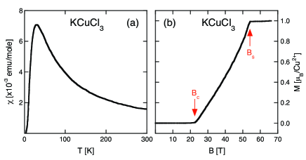
Figure 55: (a) Magnetic susceptibility measured for KCuCl₃ with $B=0.5$ T oriented perpendicular to the cleavage plane (1,0,-2). Adapted from Tanaka et al., 1997. (b) Magnetization measured for KCuCl₃ at $T=1.7$ K with $B$ perpendicular to the cleavage plane. The saturation field $B_{s}\approx 60$ T was outside the available field range. Adapted from Oosawa et al., 2002.

The state of an individual dimer at position ${\bf r}$ is well approximated by a linear combination of the singlet $|0,0\rangle$ and the triplet $|1,+1\rangle$,

$$|\Psi\rangle=u|0,0\rangle-v\exp[i({\bf k}\cdot{\bf r}-E_{+1}t)]|1,+1\rangle,$$ (98)

where $E_{+1}$ is defined by Eq. (VI.2), and the amplitudes $u$ and $v$ depend on the magnetic field Matsumoto et al. (2002, 2004). The expectation values of the spin operator components of the dimer in the state Eq. (98) are

$$\langle\hat{s}_{1,x}\rangle = -\langle\hat{s}_{2,y}\rangle\propto\frac{uv}{2}\cos({\bf k}\cdot{\bf r}-E_{+1}t),$$ (99)

$$\langle\hat{s}_{1,y}\rangle = -\langle\hat{s}_{2,x}\rangle\propto\frac{uv}{2}\sin({\bf k}\cdot{\bf r}-E_{+1}t),$$ (100)

$$\langle\hat{s}_{1,z}\rangle = -\langle\hat{s}_{2,z}\rangle\propto\frac{v^{2}}{2}.$$ (101)

The condensate at $B>B_{c}$ can be associated with the transverse order parameters $\langle\hat{s}_{i,x}\rangle$ and $\langle\hat{s}_{i,y}\rangle$ which are oppositely aligned at the dimer sites 1 and 2 due to the AFM dimer coupling $J_{0}$. The rotational symmetry $O(2)$ of the underlying spin Hamiltonian is spontaneously broken for $B>B_{c}$, giving rise to a dramatic change in the nature of the magnetic excitation spectrum. According to Eq. (VI.2), the mode associated with the lowest triplet $|1,+1\rangle$ exhibits a quadratic dispersion around the wave vector ${\bf k}_{0}=(\pi/a,\pi/a)$ and becomes gapless at the critical field $B_{c}$, but for $B>B_{c}$ it transforms in a fully isotropic system into a gapless Goldstone mode with a sound-like, linear dispersion

$$E({\bf k}) = \hbar s|{\bf k}-{\bf k}_{0}|$$ (102)

where $s$ is a velocity Matsumoto et al. (2002, 2004).

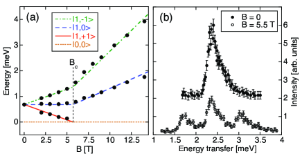
Figure 56: (Color online) Selected results obtained from INS experiments on TlCuCl₃. (a) Field dependence of the magnetic excitation energies measured at ${\bf Q}=(0,4,0)$. The solid lines reflect a linear Zeeman model. The critical field is $B_{c}=5.7$ T. Adapted from Rüegg et al., 2003. (b) Splitting of the singlet-triplet excitation measured at ${\bf Q}=(-0.5,0,2)$ and $T=1.5$ K. The asymmetric line shapes are typical resolution effects. Adapted from Cavadini et al., 2002.

One of the most widely studied dimer-based antiferromagnets is the monoclinic compound TlCuCl₃ in which the Cu²⁺ ions are arranged in centro-symmetric pairs. The intra-dimer coupling $J_{0}=-2.7$ meV dominates the inter-dimer couplings $|J_{1}|<1$ meV. INS experiments confirmed the singlet-triplet nature of the magnetic excitations by applying an external magnetic field as visualized in Fig. 56 Rüegg et al. (2003). For $B>0$ the singlet-triplet excitation is clearly split into three lines due to the Zeeman effect, with the central $\Delta M=0$ line being twice as intense as the $\Delta M=\pm 1$ side lines as predicted by Eq. (18). The triplons are well characterized by a three-dimensional extension of Eq. (VI.2) with a quadratic dispersion around ${\bf Q}=(0,0,1)$ as shown in Fig. 57(a). The spin gap has a minimum value $\Delta\approx 0.70$ meV at the zone center $(0,0,1)$. With increasing field strength, the lowest triplet state $|1,+1\rangle$ reduces its energy continuously and overcomes the spin gap for a critical field $B_{c}=5.7$ T, see Fig. 56(a). Since a finite number of triplet states $|1,+1\rangle$ is created at $B_{c}$, the system undergoes a phase transition to a magnetically ordered state. This condensation of triplet states at $T\approx 0$ is therefore a prototype of a quantum phase transition.

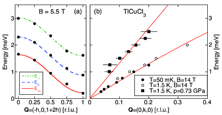
Figure 57: (Color online) (a) Energy dispersion of the triplons observed in TlCuCl₃ at $T=1.5$ K and $B=5.5$ T. The lines correspond to model expectations based on a three-dimensional extension of Eq. (VI.2). Adapted from Cavadini et al., 2002. (b) Energy dispersion of the low-lying magnetic excitations observed in TlCuCl₃ at different temperatures, fields and pressures. The lines denote the linear behavior of the Goldstone mode according to Eq. (102). Adapted from Rüegg et al., 2003; Rüegg et al., 2004b.

What is the experimental proof that TlCuCl₃ is Bose-Einstein condensed at $B_{c}$? Important evidence is provided by the critical exponent $\phi$ in the field dependence of the critical temperature, $T_{c}(B)\propto(B_{c}-B)^{\phi}$. The theory for a three-dimensional Bose gas predicts a universal value $\phi=2/3$ (see, e.g. Giamarchi and Tsevlik, 1999), which was experimentally confirmed, e.g., for the dimer compounds BaCuSi₂O₆ Jaime et al. (2004) and TlCuCl₃ Tanaka et al. (2007) in some temperature range. The ultimate proof for the Bose-Einstein condensation in TlCuCl₃, however, is offered by the properties of the magnetic excitation spectrum above $B_{c}$ according to Eq. (102). This theoretical prediction was observed for the first time by INS experiments in TlCuCl₃ as shown in Fig. 57(b) Rüegg et al. (2003), thus the presence of a spin-wavelike mode with a linear dispersion is a convincing signal for the existence of the Bose-Einstein condensate.

The singlet-triplet gap of TlCuCl₃ can also be closed by the application of hydrostatic pressure (thereby modifying the parameter $\gamma$) which occurs at a critical pressure $p_{c}\approx 0.1$ GPa. In contrast to the field induced case, all the triplet components can condense into the singlet ground state at the quantum critical point $p_{c}$. The magnetic excitation spectrum has again the nature of a gapless Goldstone mode Matsumoto et al. (2004) which was experimentally confirmed in the pressure-induced ordered phase as shown in Fig. 57(b) Rüegg et al. (2004a). In later INS experiments, it was demonstrated that only the longitudinal and one transverse triplet component soften at $p_{c}$, whereas the other transverse triplet component retains a finite gap at $p_{c}$ Rüegg et al. (2008). For $p>p_{c}$, the gap energies of both transverse components remain constant, whereas that of the longitudinal component gradually increases. The data could consistently be interpreted by using a mainly linear pressure dependence of the exchange parameters as well as a tiny exchange anisotropy. The gap energy of the longitudinal mode increases with the ordered magnetic moment above $p_{c}$, with a fundamental ratio of $\sqrt{2}$ between the gaps in the ordered and disordered states, thereby providing a non-trivial experimental test of the $S_{\varphi}$ field theory Sachdev (2011). Such an amplitude mode is not present in a classical description of ordered magnets, but is a direct consequence of the underlying quantum criticality.

Up to the present, the compound TlCuCl₃ has remained a prototype of a quantum antiferromagnet in which evidence for the Bose-Einstein condensation was given by many techniques. The concept of a Bose-Einstein condensation has been applied to some other dimer based compounds mentioned in Sec. VI.1 as well, but often factors such as the large values of the exchange parameters as well as the presence of anisotropies violating the rotational symmetry prevent the complete softening of the lowest triplet component $|1,+1\rangle$ at $B_{c}$. The influence of anisotropies, which can be determined rather precisely by EPR techniques (see, e.g., Kolezhuk et al., 2004), was discussed elsewhere Giamarchi et al. (2008).

Dimerized antiferromagnetic chain systems are closely related to the ACuCl₃ (A = K, Tl) compounds discussed above. A well studied example is copper nitrate, Cu(NO₃)₂$\cdot$2.5(D₂O), in which the spin-1/2 Cu²⁺ ions are arranged as chains of copper pairs. Each pair has a singlet ground state separated from a triplet at $|2J_{0}|=0.44$ meV. The weak interdimer coupling $J_{1}=J_{0}/\gamma$ with $\gamma\approx 4$ yields triplet excitations that propagate coherently along the chain Xu et al. (2000). The experimental data displayed in Fig. 58 are well described by the one-dimensional variant of Eq. (VI.2) with ${\bf k}=(k_{x},0)$ where $x$ denotes the chain direction. Above the singlet-triplet gap there is a second gap to the multimagnon continuum. Two-magnon bound states with $S=1$ are visible in INS experiments Tennnant et al. (2003); Tennant et al. (2012) and have a dispersion Uhrig and Schulz (1996); Schmidt and Uhrig (2003)

$$E_{BS}({\bf k})=-2J_{0}-\frac{J_{1}}{2}[1+4\cos^{2}(k_{x}d)],$$ (103)

as shown in Fig. 58. These $S=1$ bound states exist only over the range $|n\pi-k_{x}d|\leq\pi/3$, where $n$ is an odd integer.

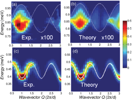
Figure 58: (Color online) Excitation spectra of copper nitrate at $T=0.12$ K. Panels (a) and (c) show background-subtracted two- and one-magnon INS data, respectively, while panels (b) and (d) show the simulated $T=0$ spectra. Adapted from Tennant et al., 2012.

VI.3 Spin-Peierls dimerization

For a compound built up by identical atoms the elastic energy is lowest if the atoms are equally spaced. However, there are compounds where the atoms move from an equally-spaced crystal to one in which the spacing alternates, i.e., the atoms form pairs. This is called dimerization (first proposed for one-dimensional systems by Peierls in the 1930s in a textbook entitled ”Quantum theory of solids”), which is made possible through lowering of the free energy of the electronic subsystem by this maneuver. The early examples mainly included polymer-like organic materials, characterized by antiferromagnetic Heisenberg chains, being first discovered in the compound TTF-CuS₄C₄(CF₃)₄ Bray et al. (1975) and afterwards in MEM-(TCNQ)₂ Huizinga et al. (1979) and in DEM-(TCNQ)₂ Schwerdtfeger et al. (1982). Here we exemplify the phenomenon of a spin-Peierls transition for the linear-chain compound CuGeO₃ Nishi et al. (1994), followed by a discussion of the three-dimensional compound CeRu₂Al₁₀, in which recently a dimerization has been suggested to occur Robert et al. (2010).

CuGeO₃ is a linear Cu²⁺ ($s_{i}=1/2$) chain compound crystallizing in the orthorhombic space group $Pbmm$ with $a=4.81$ Å, $b=8.47$ Å, and $c=2.941$ Å at room temperature Völlenkle et al. (1967). The coupling of the Cu²⁺ ions positioned at (1/2,0,0) is strong along the $c$ axis giving rise to physical properties typical of a one-dimensional magnet. The magnetic susceptibility rapidly drops to zero below $T_{c}=14$ K Hase et al. (1993), which points to the opening of a finite energy gap associated with a singlet ground state. This can be understood in terms of lattice dimerization, i.e., the formation of Cu²⁺ pairs resulting in a spin-Peierls ground state. Neutron diffraction experiments indeed gave evidence for Cu-Cu dimerization along the c axis below $T_{c}$ with an interatomic separation of 2.926 Å, compared to 2.941 Å in the high-temperature structure Hirota et al. (1994), accompanied by shifts in the position of the O(2) ions in the $(a,b)$ plane as illustrated in Fig. 59. Since the coupling between two Cu²⁺ ions in the $c$ direction is mainly due to a superexchange interaction through O(2), the dimerization is clearly driven by the O(2) shifts, which results in two unequal and alternating exchange parameters along the $c$ direction:

$$J_{1,2}(T)=J_{c}\left[1\pm\delta(T)\right].$$ (104)

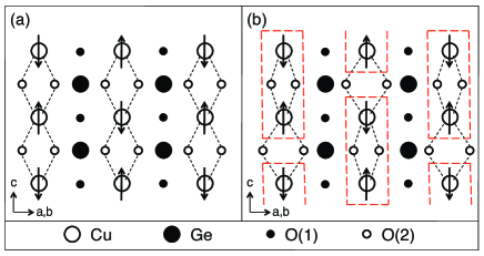
Figure 59: (Color online) Schematic representation of the structure of CuGeO₃. The arrows denote the AFM spin alignment of the Cu²⁺ ions. The dashed lines mark the Cu-O(2)-Cu superexchange bonds. (a) $T>T_{c}=14$ K. (b) Copper dimerization for $T<T_{c}$ indicated by the dashed boxes.

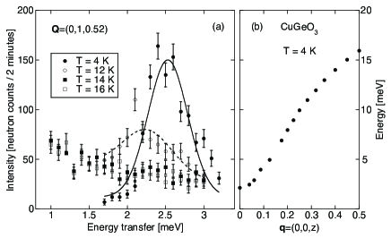
Figure 60: (a) Energy scan profiles of the magnetic excitation observed for CuGeO₃ at ${\bf Q}=(0,1,0.52)$ for various temperatures. The full and dashed lines denote Gaussian fits to the data obtained at $T=4$ and 12 K, respectively. (b) Dispersion of the magnetic excitation observed in CuGeO₃ along the $c$ direction at $T=4$ K. Adapted from Nishi et al., 1994.

The existence of the spin-Peierls gap was verified by INS experiments as shown in Fig. 60(a) Nishi et al. (1994). At $T=4$ K a sharp peak corresponding to the singlet-triplet transition appears at an energy transfer of 2.5 meV for ${\bf Q}=(0,1,0.52)$ which is close to the Brillouin zone center $(0,1,0.5)$. With increasing temperature the peak moves to lower energies and broadens ($T=12$ K), while at $T=T_{c}=14$ K the energy gap vanishes as expected. The dispersion of the singlet-triplet transition is shown in Fig. 60(b). The energy at the zone boundary ($z=1/2$) yields directly the intra-chain exchange parameter $J_{c}=10.4$ meV from the formula $\pi J_{c}/2=16.3$ meV derived by Des Cloizeaux and Pearson Des Cloizeaux and Pearson (1962). This information is useful to derive the value of $\delta(T)$ in Eq. (104). The mean-field theory gives

$$\delta(T)=\frac{\Delta(T)}{pJ_{c}},$$ (105)

with $p=1.637$ Bray et al. (1975). Substituting $\Delta(0)=2.1$ meV by extrapolation of the gap energy $\Delta(4K)=2.5$ meV [see Fig. 60(a)] to zero temperature yields $\delta(0)=0.12$ and $J_{1}(0)/J_{2}(0)=1.27$ from Eq. (104).

Recently the ternary compound CeRu₂Al₁₀ has attracted much attention because of a phase transition taking place at $T_{0}=27$ K whose origin remained unclear initially Strydom (2009). CeRu₂Al₁₀ crystallizes in the orthorhombic space group $Cmcm$ in which the Ce³⁺ ions are separated from each other by an exceptionally large distance of 5.2 Å, so that the interpretation of $T_{0}$ as a magnetic phase transition has to be discarded. Alternative mechanisms such as a charge-ordered state as well as spin-density-wave formation also have serious shortcomings Nishioka et al. (2009); Matsumara et al. (2009). Tanida et al. (2010b, a) suggested the formation of Ce dimers within the $(a,c)$ plane, bearing some similarities to a spin-Peierls transition. Neutron scattering experiments confirmed the latter interpretation Robert et al. (2010). Neutron diffraction measurements gave evidence for a displacement of the Al atoms below $T_{0}$, resulting in a spin-Peierls transition along the one-dimensional Ce-Al zig-zag chains accompanied by a dimerization of the Ce³⁺ ions as sketched in Fig. 61.

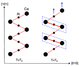
Figure 61: (Color online) Schematic representation of the Ce-Al zig-zag chains in CeRu₂Al₁₀. The Ce³⁺ dimerization for $T<T_{0}$ is indicated by the dashed boxes.

The final proof of the Ce³⁺ dimerization is provided by the results of INS experiments performed for CeRu₂Al₁₀ as shown in Fig. 62(a) Robert et al. (2010). At temperatures $T<T_{0}$ there is no spectral weight at low energies. There is a well defined peak at 8 meV corresponding to the gap energy. With increasing temperature the gap shifts to lower energies. The peak at 8 meV can therefore be identified as the singlet-triplet excitation associated with the formation of Ce³⁺ dimers below $T_{0}$ which is supported by the oscillatory $Q$ dependence of the intensities according to the dimer cross-section Eq. (3.9) as illustrated in Fig. 62(b). From the peak position and Eq. (3.3) the effective intra-dimer exchange coupling results as $J_{eff}=-4$ meV, which was considered to be unrealistically large Robert et al. (2010). However, this value is based on a truncated basis with $s=1/2$. The true exchange coupling between the Ce³⁺ ions results from scaling with the de Gennes factor $\xi=(g-1)^{2}j(j+1)$, where $j$ is the total angular momentum. For Ce³⁺ with $g=6/7$ and $j=5/2$ we have $\xi=0.18$, and for an $s=1/2$ system ($g=2$, $j=1/2$) we find $\xi=0.75$, thus the correction by the de Gennes factor reduces the true exchange coupling to $J_{Ce-Ce}\approx-1$ meV.

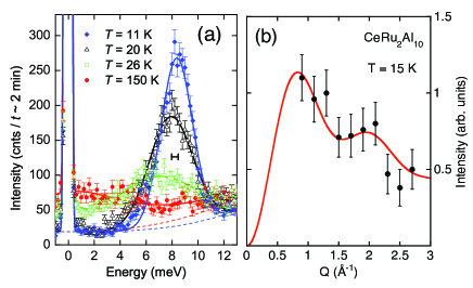
Figure 62: (Color online) (a) Temperature dependence of the energy spectra of neutrons scattered from CeRu₂Al₁₀ for $Q=1.5$ Å^-1. The lines denote least-squares fits. (b) $Q$ dependence of the intensity of the peak at 8 meV. The line corresponds to the dimer cross-section Eq. (3.9) with $R=5.2$ Å. Adapted from Robert et al., 2010.

VI.4 Polarons

In complex materials, competing interactions can lead to the spontaneous formation of nano-sized regions of a different phase. If an additional charge is introduced into the material by doping, a fermionic quasiparticle called polaron can be formed. The resulting lattice polarization and deformation acts as a potential well that decreases the mobility of the charge. Polarons have spin, though two close-by polarons are spinless. The latter is called a bipolaron whose existence was the driving idea behind the discovery of high-temperature superconductivity in the copper-oxide perovskites Bednorz and Müller (1986). In the meantime the existence of charge-ordered stripes was postulated Zaanen and Gunnarsson (1989) and experimentally verified Lucarelli et al. (2003). The stripes are superconducting regions, separated by AFM regions which act as Josephson junctions by the proximity effect.

The existence of polarons is the key to understand the rich phase diagrams of the giant-magnetoresistive manganese and cobalt perovskites upon doping Salamon and Jaime (2001); Phelan et al. (2006). This is demonstrated here for the hole-doped lanthanum cobaltates of type La_1-xSr_xCoO₃. The ground state of the parent compound LaCoO₃ is nonmagnetic, corresponding to a low-spin state of Co³⁺ ions with $s_{i}=0$. It was widely believed that the addition of each hole into pristine LaCoO₃ through the substitution of a Sr²⁺ ion for the La³⁺ ion creates a Co⁴⁺ ion in the lattice which has a nonzero value of $s_{i}$ in any spin-state configuration, thereby inducing a magnetic moment in the system. However, already lightly doped cobaltates with $x\approx 0.002$ give rise to an order of magnitude larger magnetic susceptibility than expected Yamaguchi et al. (1996). It was proposed that the holes introduced by Sr doping do not remain localized at the nearby Co site, but each hole is distributed among several neighboring Co sites, leaving the latter in the intermediate Co³⁺ state (with $s_{i}=1$) and thereby forming a multi-site magnetic polaron. Such spin-state polarons behave like ferromagnetic nanoparticles with a very large total spin in an insulating nonmagnetic matrix.

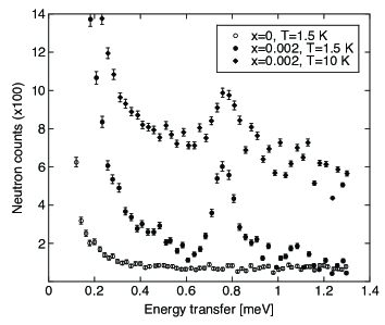
Figure 63: Energy spectra of neutrons scattered from La_0.998Sr_0.002CoO₃ at $T=1.5$ and 10 K. The open circles correspond to the nonmagnetic reference compound LaCoO₃. For clarity, the intensities of the $T=10$ K data are shifted by 400 neutron counts. Adapted from Podlesnyak et al., 2008.

The existence of spin-state polarons was confirmed by inelastic neutron scattering experiments as shown in Fig. 63. A magnetic excitation is observed for La_0.998Sr_0.002CoO₃ at an energy transfer of 0.75 meV, which is absent for the undoped parent compound LaCoO₃ Podlesnyak et al. (2008). The ground state of Co³⁺ in the intermediate spin state is an orbitally degenerate triplet which is split by a small trigonal ligand field into a singlet and a doublet. The transition between these two levels is the source of the peak observed at 0.75 meV. The peak intensity diminishes with increasing temperature, in agreement with the Boltzmann population factor Eq. (45) for a singlet-doublet transition. The $Q$ dependence of the intensity of the observed excitation exhibits a clear oscillatory behavior as shown in Fig. 64, which reflects the size as well as the shape of the polaron through the structure factor. The neutron cross-section of a cluster comprising $N$ magnetic ions can be approximated for polycrystalline material by an extension of Eq. (34):

$$\frac{d^{2}\sigma}{d\Omega d\omega} \propto F^{2}(Q)\sum_{i<j=1}^{N}[\langle S||\hat{T}^{(1)}(s_{i})||S^{\prime}\rangle^{2}+2\frac{\sin(QR_{ij})}{QR_{ij}}$$ (106)

$$\times\langle S||\hat{T}^{(1)}(s_{i})||S^{\prime}\rangle\langle S^{\prime}||\hat{T}^{(1)}(s_{j})||S\rangle],$$

For the special case of a $\Delta S=0$ transition (which is relevant in the present context), the reduced matrix elements can be factorized and set to 1. The lines in Fig. 64 correspond to calculated cross sections for different Co clusters sketched in the insert. We clearly see that the $Q$ dependence of the cross section is an unambiguous fingerprint of the geometry of the multimers; in particular, the data observed for the 0.75 meV transition in La_0.998Sr_0.002CoO₃ are perfectly explained by the scattering from an octahedrally shaped Co heptamer. The total moment of this heptamer, consisting formally of one central Co⁴⁺ ion ($s_{i}=1/2$) and six surrounding Co³⁺ ions ($s_{i}=1$), is 13 $\mu_{B}$, in good agreement with the magnetic susceptibility data Yamaguchi et al. (1996).

The result of the above experiment gives a clear microscopic explanation why hole doping of as little as 0.2% dramatically affects the overall magnetic properties of the entire system, i.e., the magnetic susceptibility is an order of magnitude larger than expected. Additional charge carriers increase the number of such spin-state polarons, which form a percolative network resulting in a metallic state with long-range ferromagnetic order at the critical Sr concentration $x_{c}=0.18$ Phelan et al. (2006). The formation of spin-state polarons may be a common mechanism present in other Mn- and Co-based oxide perovskites as well.

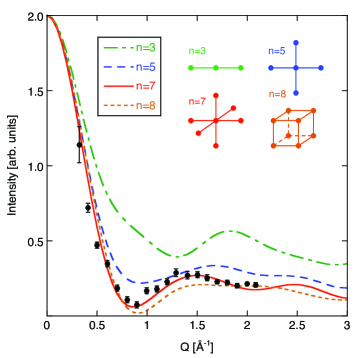
Figure 64: (Color online) $Q$ dependence of the intensity of the transition observed at 0.75 meV in La_0.998Sr_0.002CoO₃. The insert sketches different types of Co multimers. The lines are the result of structure factor calculations based on Eq. (106). Adapted from Podlesnyak et al., 2008.

VII Conclusions

In this review we have attempted to provide an impression of the physics which one encounters in magnetic spin clusters, and their relevance to a variety of different physical systems. The presentation had obviously been limited to examples whose magnetic excitations have already been very well or comparatively well understood. Many of the important scientific questions which are under current research or will possibly become of relevance in future have however not been addressed, though some of them were indicated at few places in the text. We wish to conclude here by picking them up again.

The small magnetic clusters have been demonstrated to be ideal experimental systems for studying the basic mechanisms of the magnetic interactions between spins and the underlying physical principles. The research on them started at least six decades ago and many fundamental questions could be addressed (Sec. III). However, despite this long history, the research field is not yet exhausted, but continuously increases due to the ongoing improvements of the experimental equipment. For instance, for many fascinating extended magnetic compounds the corrections to the HDVV model such as the weaker anisotropic and/or higher-order exchange interactions have to be known with accuracy as they can be crucial for understanding their phase diagrams. However, the higher-order interactions are intrinsically hidden in the commonly applied analyzes of spin-wave dispersion relations, but become accessible by studying the cluster excitation spectra in the related diluted materials; an example was given in Sec. III.2.6.

For most magnetic systems the conventional HDVV model, possibly including the weaker corrections to it, is perfectly appropriate, which is not surprising for magnetic ions of type S and type Q. The basic assumptions underlying the HDVV picture are phenomenological, but there was little clear-cut experimental evidence in the past for an eventual failure of this model. The situation is quite different for clusters with magnetic type L and type J ions, and the exchange in general has to be described by more involved interaction terms. An obvious extension of the HDVV coupling is to introduce multipole interactions based on standard tensor operator techniques or to replace the exchange parameter $J_{ij}$ by an exchange tensor $J(m_{i},m_{j};m^{\prime}_{i},m^{\prime}_{j})$, with $m_{i}$ and $m^{\prime}_{i}$ being the spin quantum numbers of the initial and final ionic states, respectively; the latter formalism was verified in the dimeric Ho³⁺ compound Cs₃Ho₂Br₉ Furrer et al. (1990). This topic will certainly become more important in the future, e.g., magnetic molecules incorporating 4f metal ions are currently intensely studied Klokishner et al. (2009a).

The observed existence of three-spin interactions in magnetic systems discussed in Sec. III.2.5 is of particular relevance in the general context of many-body interactions, which already fascinated Kopernikus (1473-1543) and Kepler (1571-1630) in their investigations of the mutual gravitational interaction between three planets. There has been ample experimental evidence for many-body interactions in the past, notably in studies of ultra-cold gases of alkaline atoms Büchler et al. (2007), the stability of molecules like ozone Zhaunerchyk et al. (2007), four-atom exchange in ³He McMahan and Wilkins (1975), chirality in magnetic compounds Grigoriev et al. (2005), ring-exchange Coldea et al. (2001) and three-body correlations of vortex states Menon et al. (2006) in high-temperature superconductors, or domain-wall fluctuations in (anti-) ferromagnets Shpyrko et al. (2007). Novel quantum phases with intriguing physical properties can arise from many-body interactions which are usually described on the basis of pair potentials $G({\bf r},t)$. However, it would be highly desirable to extend the analytic tools beyond van Hove’s theory van Hove (1954) to include higher-order correlation functions in both space and time, for which approximate solutions exist, e.g., for $G({\bf r},{\bf r}^{\prime},t)$ Hu (2007), $G({\bf r},t,t^{\prime})$ Word and Trammell (1981) and $G({\bf r},{\bf r}^{\prime},t,t^{\prime})$ van Zon and Schofield (2001). Adequate experimental techniques should be developed as well which provide a direct access to higher-order correlation functions. Indeed, novel neutron scattering techniques were suggested for this purpose which include neutron interferometry Rauch and Suda (1998) and spin-echo techniques Grigoriev et al. (2004).

Besides the small magnetic clusters the ground state and excitation spectrum in the large magnetic clusters, as they have been called in this review, has emerged as an attractive research field in the last 15 years. The scientific questions encountered in them are ultimately related to the possibility of many-body (quantum) effects, with links to the field of quantum spin systems. However, as compared to the system sizes considered in the latter area, in which one-, two-, and three-dimensional lattices of interacting quantum spins are considered, the sizes of the ”large magnetic clusters” have to be considered small as they are (far) away from the finite-size scaling regime, in which the magnetic properties start to resemble those in the thermodynamic limit $N\rightarrow\infty$ (exceptions are spin-1/2 clusters because of the short correlation length for $s_{i}=1/2$, see Sec. IV.3 and Fig. 28). In this sense the large magnetic clusters should be called zero dimensional and belong to the class of mesoscopic systems.

A typical consequence of that could be described as the ”loss” of the wave vector as a good quantum number, since translational symmetry or a finite-size version of it such as the cyclic symmetry in wheels is generally not present in the large clusters. On the one hand this implies that concepts which are developed for extended lattices may have to be adapted or interpreted in novel ways if applied to the large clusters. The application of spin-wave theory to the antiferromagnetic wheels and short chains (Secs. IV.3.1 and IV.4.2) represents a showcase.

For the antiferromagnetic Heisenberg rings or molecular wheels the cyclic symmetry allows introducing a shift quantum number $q$ which emerges into a wave vector in the thermodynamic limit. Therefore the available literature results for the spin-wave dispersion relation in the antiferromagnetic chain, as they have been derived from the various spin-wave theories Ivanov and Sen (2004), can be taken over directly with the wave vector replaced by the discrete values of $q$. As was demonstrated in Sec. IV.3.2 for the CsFe₈ molecular wheel this yields the energies in the $E$ band with some accuracy. However, besides this success, fundamental issues are eminent. For instance, spin-wave theories do a priori violate the spin rotational invariance of the HDVV Hamiltonian, and their applicability to large clusters with their disordered ground states is hence fundamentally flawed, yet they can produce reasonable energies and one may ask why. Also, since the wave vector becomes discretized, magnetic excitations with long wave lengths do not exist in molecular wheels (and large magnetic clusters in general), which raises the question of whether the excitations in the $E$ band, albeit their energies can be derived by spin-wave theory, should actually be interpreted as spin waves. This is a sensible question, and the notion of ”cluster spin waves” may be introduced Stuiber et al. (2011). We here adopted a pragmatic view and called any excitation which is obviously related to a spin-wave energy a spin wave.

The situation becomes even more involvled in the short antiferromagnetic chains. At the level of linear spin-wave theory the literature result for the finite antiferromagnetic chain can again directly be carried over, but this does not work for the more sophisticated spin-wave theories such as interacting spin-wave theory since the open boundaries result in site dependent corrections. That is, these theories have to be formulated in real space and not momentum space. Furthermore, a description of the excitations in classical terms, which is at the heart of the $L\&E$-band concept and motivated applying spin-wave theories, is actually not obvious in the short chains as the wave functions do not significantly overlap with the semiclassical configurations. Surprisingly, their ground state is in fact neither in the classical nor the quantum regime and the intuitively clear distinction between these two regimes becomes blurred Konstantinidis et al. (2011).

The loss of the wave vector on the other hand is also indicative of the possibility of lattice topologies in large clusters which are not possible in extended systems. In fact, most magnetic molecules which were synthesized have a complex topology which cannot systematically be expanded into an infinite lattice. The V₁₅ or Mn₁₂ molecules presented in Secs. IV.5.1 and V.2 are examples. However, for obvious reasons, the research on the many-body aspects of magnetic cluster excitations concentrated on lattice topologies or magnetic molecules with an ”appealing” symmetry, but the most interesting magnetic phenomena may be overlooked this way. In this sense only the simplest systems were studied so far, yet the understanding of their excitations can be challenging and the case of Fe₃₀ establishes a dramatic example. The large number of lattice topologies available through the molecular nanomagnets, which thanks to the productivity of chemists will certainly grow further, presents obviously a wide area for future research.

Except of two cases Waldmann et al. (2006a); Carretta et al. (2007) (see also Sec. IV.5.1) the INS works on molecular nanomagnets were using powder/polycrystalline samples. Experiments on single crystals would offer new possibilities to unravel the many-body physics in the cluster excitations, e.g., the spin-pair correlation function can be mapped out more directly than possible with powder samples. Single-crystal INS experiments have become state of the art in the last decade for inorganic compounds. The current drastic improvements in the INS technique make such experiments possible now also for molecular nanomagnets (which are challenging because of the small number of magnetic centers as compared to the many non-magnetic ligand atoms). Single-crystal INS work on molecular nanomagnets will certainly been seen more often in the next years.

Magnetic cluster systems have also been considered as promising units for quantum computing. Much effort went into ”mesoscopic spin-1/2 clusters” or ”antiferromagnetic cluster qubits”, i.e., large clusters which exhibit a total spin $S=1/2$ ground state and may be used as qubits at low temperatures, where only the ground state is thermally populated Meier et al. (2003a, b). Such clusters may present advantages over atomic scale qubits, such as easier addressing and readout. Significant progress were made, e.g., coherence times long enough for quantum computations could be achieved in the Cr₇Ni ”doped” antiferromagnetic wheel Ardavan et al. (2007) and two molecular ”qubits” could be linked such as to provide entanglement between them suggesting the possibility of two-qubit operations Candini et al. (2010); Affronte et al. (2005, 2006). However, the multi-level structure of the low-lying energies as it can be provided only by magnetic clusters has also been explored. The particular structure of the ground-state spin multiplet in the single-molecule magnets was theoretically shown to allow for an implementation of Grover’s search algorithm or to build dense and efficient memory devices Leuenberger and Loss (2001). Furthermore, by accessing also higher-lying levels nearby to the ground state Rabi oscillations could be observed in the V₁₅ molecule and the Fe₄ single-molecule magnet Bertaina et al. (2008); Schlegel et al. (2008). Lastly, the spin frustration or orbital degeneracy in the ground state of regular spin triangles has been theoretically shown to allow for a coupling of the spin degree of freedom to electric fields and currents (spin-electric currents), such that the spin qubit can be manipulated through currents supplied to a cluster by e.g. scanning tunneling microscope (STM) techniques Trif et al. (2008); Lehmann et al. (2007); Georgeot and Mila (2010). These examples indicate that the cluster excitations as present in magnetic clusters may provide novel quantum computation schemes, and exciting results in this direction can be expected in the future. For instance, the many-body nature of the large magnetic clusters suggests the possibility of decoherence free subspaces in them, which however has to our knowledge not yet been explored.

Magnetic clusters play also a role in the emerging field of molecular spintronics Bogani and Wernsdorfer (2008); Sanvito and Rocha (2006); Rocha (2005). Significant success has first been obtained with molecules containing one metal ion, which have been incorporated into break junctions or contact leads produced by electro migration. For instance, the Kondo effect could be observed in the molecule [Co(terpy(CH₂)₅-SH)₂]²⁺ this way Park et al. (2002). However, also the current-voltage characteristics of magnetic clusters of two metal centers or even the single-molecule magnet Mn₁₂ have been measured in experiment Heersche (2006). Many further schemes are currently under investigation Bogani and Wernsdorfer (2008). As in the context of quantum computation it can also be envisioned for molecular spintronics that the unique energy level structures or complex many-body states provided by magnetic cluster systems will open novel opportunities and allow for functionalities not currently considered.

The molecular nanomagnets represent obviously a valuable resource of (large) magnetic clusters, but in the recent years not only the chemical route towards large clusters has been advanced, but several beautiful examples of artificially engineered spin clusters also emerged Jamneala et al. (2001). Here ensembles of magnetic metal ions experiencing nearest-neighboring exchange interactions were fabricated directly on surfaces using STM techniques, and their magnetic excitations measured through recording the current-voltage curves. For instance, short antiferromagnetic chains of Mn²⁺ metal ions with chain lengths of $N=1-10$ were produced and the magnetic ground state as well as first excited excitation observed this way Hirjibehedin et al. (2006). Apparently in both areas, that of the molecular nanomagnets and the artificially engineered spin clusters, one faces very similar scientific questions, yet the technological challenges in putting them forward in real-world applications are complementary. In comparison with the artificially formed clusters, the molecular nanomagnets are available in an abundance of different lattice topologies assuming complex many-body states and their excitations can be studied in any detail using powerful experimental techniques such as inelastic neutron scattering. However, the artificial nanostructures are available directly on surfaces and have already been proven to maintain their magnetic properties and their function to be addressable on the surface. The molecular nanomagnets and the artificially engineered spin systems are hence complementary in the sense that the advantages of each class may help the other to overcome its problems Konstantinidis et al. (2011).

Furthermore, magnetic cluster excitations are fundamental in a variety of other systems. For instance, the clusters may be linked together by a network of weak magnetic inter-cluster exchange interactions, such that the cluster excitations may ”travel” through the network and become dispersive. This can lead to fascinating novel quantum phases, and the Bose-Einstein condensation in the dimer-based compounds, which was presented in Sec. VI.2, is a striking example. However, such networks may obviously not only be built from dimers, but also trimers or tetramers, which can additionally introduce spin frustration and possess unprecedented behavior. At this point a further link between molecular nanomagnets and quantum spin systems emerges, as not only small clusters may be incorporated into the network but also large clusters or molecular nanomagnets, which should be expected to result in an interesting interplay between the complex quantum states realized within a cluster and the complex phases generated in extended lattices. Indeed, the synthesis of extended exchange-coupled networks of, e.g., Cu₃ molecular units or single-molecule magnets have already been reported Ivanov et al. (2010); Morimoto et al. (2009); Miyasaka et al. (2006). All in all, the competition between the quantum states in a magnetic cluster and the cooperativity introduced through an extended network of inter-cluster interactions should continue to be an attractive playground for research.

Lastly, clusters of magnetic ions are relevant in biology as they constitute the active sites in many metalloproteins. They are ubiquitous in living matter and contain sites with one to eight metal atoms, sometimes with multiple occurrence of the smaller clusters in the same protein molecule. The primary function of, e.g., the iron-sulfur clusters lies in mediating one-electron redox processes and as such they are integral components of respiratory and photosynthetic electron transfer chains. So far the understanding of the electronic ground- and excited-state properties relied on magnetic susceptibility, magnetic circular dichroism, EPR, Mössbauer and resonance Raman scattering measurements, which provided information on the anisotropy of the $g$ factor, the valence state of the iron atoms, the total spin quantum number of the ground state, and sometimes the intra-cluster exchange interactions Beinert et al. (1997). The latter are often determined from experiments on model systems as demonstrated, e.g., by magnetic susceptibility measurements of a cubane-type Fe₄S₄ cluster, giving $J=-18$ meV for the exchange parameter of the two semi-independent (Fe₂S₂)²⁺ dimers Yoo et al. (1997). To our knowledge, the very informative INS technique has not yet been applied to the study of metalloproteins, since prohibitively large deuterated samples with volumes of typically 1 cm³ would be needed. However, with the advent of third-generation neutron sources and novel beam-focusing techniques, reducing the requested sample size by several orders of magnitude, such experiments will become feasible in the near future.

As so often, improvements in the experimental techniques are a main driving force for scientific progress, and it is finally mentioned that the development of the instrumentation used for studying magnetic cluster excitations has been impressive in the last decade, and should be expected to be so also in the future. Neutron scattering can serve as a representative example. Neutron facilities such as the high-flux reactor HFR at the Institute Laue-Langevin (ILL) in Grenoble (France) and the spallation neutron source ISIS at the Rutherford Appleton Laboratory in Didcot (U.K.) which both presently undergo significant upgrades as well as the successful commissioning or planing of new third-generation neutron sources such as the Spallation Neutron Source (SNS) at the Oak Ridge National Laboratory (USA), the spallation neutron source at J-PARC in Tokai (Japan), and the European Spallation Source (ESS) in Lund (Sweden) open truly exciting perspectives to unravel the many unsolved questions in the area of magnetic cluster excitations.

References

- Abbati et al. (2001) Abbati, G. L., L.-C. Brunel, H. Casalta, A. Cornia, A. C. Fabretti, D. Gatteschi, A. K. Hassan, A. G. M. Jansen, A. L. Maniero, L. Pardi, C. Paulsen, and U. Segre, 2001, Chem. Eur. J. 7, 1796.
- Abragam and Bleaney (1986) Abragam, A., and B. Bleaney, 1986, Electron Paramagnetic Resonance of Transition Ions (Dover Publications, Inc., New York).
- Affleck et al. (1987) Affleck, I., T. Kennedy, E. H. Lieb, and H. Tasaki, 1987, Phys. Rev. Lett. 59, 799.
- Affronte et al. (2007) Affronte, M., S. Carretta, G. A. Timco, and R. E. P. Winpenny, 2007, Chem. Commun. , 1789.
- Affronte et al. (2005) Affronte, M., I. Casson, M. Evangelisti, A. Candini, S. Carretta, C. A. Muryn, S. J. Teat, G. A. Timco, W. Wernsdorfer, and R. E. P. Winpenny, 2005, Angew. Chem. Int. Ed. 44, 6496.
- Affronte et al. (2006) Affronte, M., F. Troiani, A. Ghirri, S. Carretta, P. Santini, V. Corradini, R. Schuecker, C. Muryn, G. Timco, and R. E. P. Winpenny, 2006, Dalton Trans. , 2810.
- Amiri et al. (2010) Amiri, H., A. Lascialfari, Y. Furukawa, F. Borsa, G. A. Timco, and R. E. P. Winpenny, 2010, Pyhs. Rev. B 82, 144421.
- Amoretti et al. (2001) Amoretti, G., S. Carretta, R. Caciuffo, H. Casalta, A. Cornia, M. Affronte, and D. Gatteschi, 2001, Phys. Rev. B 64, 104403.
- Anderson (1952) Anderson, P. W., 1952, Phys. Rev. 86, 694.
- Anderson (1984) Anderson, P. W., 1984, Basic Notions of Condensed Matter Physics (Benjamin/Cummings Pubkishing Co., Menlo Park).
- Ardavan et al. (2007) Ardavan, A., O. Rival, J. J. L. Morton, S. J. Blundell, A. M. Tyryshkin, T. G. A., and R. E. P. Winpenny, 2007, Phys. Rev. Lett. 98, 057201.
- Awschalom et al. (1992) Awschalom, D. D., J. F. Smyth, G. Grinstein, D. P. DiVincenzo, and D. Loss, 1992, Phys. Rev. Lett. 68, 3092.
- Axenovich and Luban (2001) Axenovich, M., and M. Luban, 2001, Phys. Rev. B 63, 100407R.
- Azuma et al. (1994) Azuma, M., Z. Hiroi, M. Takano, K. Ishida, , and Y. Kitaoka, 1994, Phys. Rev. Lett. 73, 3463.
- Bai et al. (2000) Bai, Z., J. Demmel, J. Dongarra, A. Ruhe, and H. vn der Horst, 2000, Templates for the Solution of Algebraic Eigenvalue Problems (SIAM, Philadelphia).
- Baker et al. (2011a) Baker, M. L., A. Bianchi, S. Carretta, D. Collison, R. J. Docherty, E. J. L. Mclnnes, A. McRobbie, C. A. Muryn, H. Mutka, S. Piligkos, M. Rancan, P. Santini, et al., 2011a, Dalton Trans. 40, 2725.
- Baker et al. (2011b) Baker, M. L., S. Piligkos, A. Bianchi, S. Carretta, D. Collison, J. J. W. McDouall, E. J. L. McInnes, H. Mutka, G. A. Timco, F. Tuna, P. Vadivelu, H. Weihe, et al., 2011b, Dalton Trans. 40, 8533.
- Baran et al. (2008) Baran, P., R. Boca, I. Chakraborty, J. Giapintzakis, R. Herchel, Q. Huang, J. E. McGrady, R. G. Raptis, Y. Sanakis, and A. Simopoulos, 2008, Inorg. Chem. 47, 645.
- Barbara et al. (2002) Barbara, B., I. Chiorescu, W. Wernsdrofer, B. Bögge, and A. Müller, 2002, Prog. Theo. Phys. Suppl. .
- Barbara and Chudnovsky (1990) Barbara, B., and E. M. Chudnovsky, 1990, Phys. Lett. A 145, 205.
- Barbara and Gunther (1999) Barbara, B., and L. Gunther, 1999, Phys. World , 35.
- del Barco et al. (2005) del Barco, E., A. D. Kent, S. Hill, J. M. North, N. S. Dalal, E. M. Rumberger, D. N. Hendrickson, N. Chakov, and G. Christou, 2005, J. Low Temp. Phys. 140, 119.
- Barra et al. (2007) Barra, A.-L., A. Caneschi, A. Cornia, D. Gatteschi, L. Gorini, L.-P. Heiniger, R. Sessoli, and L. Sorace, 2007, J. Am. Chem. Soc. 129, 10754.
- Barra et al. (1999) Barra, A. L., A. Caneschi, A. Cornie, F. Fabrizi de Biani, D. Gatteschi, C. Sangregorio, R. Sessoli, and L. Sorace, 1999, J. Am. Chem. Soc. 121, 5302.
- Basler et al. (2003) Basler, R., C. Boskovic, G. Chaboussant, H. U. Güdel, M. Murrie, S. T. Ochsenbein, and A. Sieber, 2003, Chem. Phys. Chem. 4, 910.
- Bednorz and Müller (1986) Bednorz, J. G., and K. A. Müller, 1986, Z. Phys. B - Condensed Matter 64, 189.
- Beinert et al. (1997) Beinert, H., R. H. Holm, and E. M. Münck, 1997, Science 277, 653.
- Bencini and Gatteschi (1990) Bencini, A., and D. Gatteschi, 1990, EPR of exchange coupled systems (Springer-Verlag, Berlin).
- Bernu et al. (1992) Bernu, B., C. Lhuillier, and L. Pierre, 1992, Phys. Rev. Lett. 69, 2590.
- Bertaina et al. (2008) Bertaina, S., S. Gambarelli, T. Mitra, B. Tsukerblat, A. Müller, and B. Barbara, 2008, Nature 453, 203.
- Bianchi et al. (2009) Bianchi, A., S. Carretta, P. Santini, G. Amoretti, T. Guidi, Y. Qiu, J. R. D. Copley, G. Timco, C. Muryn, and R. E. P. Winpenny, 2009, Phys. Rev. B 79, 144422.
- Bircher et al. (2006) Bircher, R., G. Chaboussant, C. Dobe, H. U. Güdel, S. T. Ochsenbein, A. Sieber, and O. Waldmann, 2006, Adv. Funct. Mater. 16, 209.
- Bircher et al. (2004) Bircher, R., G. Chaboussant, A. Sieber, H. U. Güdel, and H. Mutka, 2004, Phys. Rev. B 70, 212413.
- Bogani et al. (2004) Bogani, L., A. Caneschi, M. Fedi, D. Gatteschi, M. Massi, M. A. Novak, G. M. Pini, A. Rettori, R. Sessoli, and A. Vindigini, 2004, Phys. Rev. Lett. 92, 207204.
- Bogani and Wernsdorfer (2008) Bogani, L., and W. Wernsdorfer, 2008, Nat. Mat. 7, 179.
- Bouwen et al. (2001) Bouwen, A., A. Caneschi, D. Gatteschi, E. Goovaerts, D. Schoemaker, L. Sorace, and M. Stefan, 2001, J. Phys. Chem. B 105, 2658.
- Bray et al. (1975) Bray, J. W., H. R. Hart, L. V. Jr. Interrante, I. S. Jacobs, J. S. Kasper, G. D. Watkins, S. H. Wee, and J. C. Bonner, 1975, Phys. Rev. Lett. 35, 744.
- Breitling et al. (1977) Breitling, W., W. Lehmann, R. Weber, N. Lehner, and V. Wagner, 1977, J. Magn. Magn. Mater. 6, 113.
- Brockhouse (1955) Brockhouse, B. N., 1955, Phys. Rev. 99, 601.
- Büchler et al. (2007) Büchler, H. P., A. Micheli, and P. Zoller, 2007, Nature Physics 3, 726.
- Caciuffo et al. (1998) Caciuffo, R., G. Amoretti, A. Murani, R. Sessoli, A. Caneschi, and D. Gatteschi, 1998, Phys. Rev. Lett. 81, 4744.
- Caciuffo et al. (2005) Caciuffo, R., T. Guidi, G. Amoretti, S. Carretta, E. Liviotti, P. Santini, C. Mondelli, G. Timco, C. A. Muryn, and R. E. P. Winpenny, 2005, Phys. Rev. B 71, 174407.
- Cador et al. (2004) Cador, O., D. Gatteschi, R. Sessoli, F. K. Larsen, J. Overgaard, A.-L. Barra, S. J. Teat, G. A. Timco, and R. E. P. Winpenny, 2004, Angew. Chem. Int. Ed. 43, 5196.
- Candini et al. (2010) Candini, A., G. Lorusso, F. Troiani, A. Ghirri, S. Carretta, P. Santini, G. Amoretti, C. Muryn, F. Tuna, G. Timco, E. J. L. McInnes, R. E. P. Winpenny, et al., 2010, Phys. Rev. Lett. 104, 037203.
- Caneschi et al. (1996) Caneschi, A., A. Cornia, A. C. Fabretti, S. Foner, D. Gatteschi, R. Grandi, and L. Schenetti, 1996, Chem. Eur. J. 2, 1379.
- Carlin (1986) Carlin, R. L., 1986, Magneochemistry (Springer, Berlin).
- Carretta et al. (2008) Carretta, S., T. Guidi, P. Santini, G. Amoretti, O. Pieper, B. Lake, J. van Slageren, F. El Hallak, W. Wernsdorfer, H. Mutka, M. Russina, C. J. Milios, et al., 2008, Phys. Rev. Lett. 100, 157203.
- Carretta et al. (2004a) Carretta, S., E. Liviotti, N. Magnani, P. Santini, and G. Amoretti, 2004a, Phys. Rev. Lett. 92, 207205.
- Carretta et al. (2005) Carretta, S., P. Santini, G. Amoretti, M. Affronte, A. Ghirri, I. Sheikin, S. Piligkos, G. Timco, and R. E. P. Winpenny, 2005, Phys. Rev. B 72, 060403(R).
- Carretta et al. (2004b) Carretta, S., P. Santini, G. Amoretti, T. Guidi, R. Caciuffo, A. Candini, A. Cornia, D. Gatteschi, M. Plazanet, and J. A. Stride, 2004b, Phys. Rev. B 70, 214403.
- Carretta et al. (2007) Carretta, S., P. Santini, G. Amoretti, T. Guidi, J. R. D. Copley, Y. Qiu, R. Caciuffo, G. Timco, and R. E. P. Winpenny, 2007, Phys. Rev. Lett. 98, 167401.
- Carretta et al. (2006) Carretta, S., P. Santini, G. Amoretti, T. Guidi, J. Dyson, R. Caciuffo, J. A. Stride, A. Caneschi, and J. R. D. Copley, 2006, Phys. Rev. B 73, 144425.
- Carretta et al. (2003a) Carretta, S., P. Santini, E. Liviotti, N. Magnani, T. Guidi, R. Caciuffo, and G. Amoretti, 2003a, Eur. Phys. J. B 36, 169.
- Carretta et al. (2003b) Carretta, S., J. van Slageren, T. Guidi, E. Liviotti, C. Mondelli, D. Rovai, A. Cornia, C. F. Dearden, A. L., M. Affronte, C. D. Frost, R. E. P. Winpenny, D. Gatteschi, et al., 2003b, Phys. Rev. B 67, 094405.
- Cavadini et al. (1999) Cavadini, N., W. Henggeler, G. H. U. Furrer, A., K. Krämer, and H. Mutka, 1999, Eur. Phys. J. B 7, 519.
- Cavadini et al. (2002) Cavadini, N., C. Rüegg, A. Furrer, H. U. Güdel, K. Krämer, H. Mutka, and P. Vorderwisch, 2002, Phys. Rev. B 65, 132415.
- Cépas et al. (2001) Cépas, O., K. Kakurai, L. P. Regnault, T. Ziman, J. P. Boucher, N. M. Aso, N., H. Kageyama, and U. Y., 2001, Phys. Rev. Lett. 87, 167205.
- Cépas and Ziman (2005) Cépas, O., and T. Ziman, 2005, Prog. Theor. Phys. Suppl. 159, 280.
- Chaboussant et al. (2002) Chaboussant, G., R. Basler, A. Sieber, S. T. Ochsenbein, A. Desmedt, R. E. Lechner, M. T. F. Telling, P. Kögerler, a. Müller, and H. U. Güdel, 2002, Europhys. Lett. 59, 291.
- Chaboussant et al. (2004a) Chaboussant, G., S. T. Ochsenbein, A. Sieber, H.-U. Güdel, H. Mutka, A. Müller, and B. Barbara, 2004a, Europhys. Lett. 66, 423.
- Chaboussant et al. (2004b) Chaboussant, G., A. Sieber, S. Ochsenbein, H. U. Güdel, M. Murrie, A. Honecker, N. Fukushima, and B. Normand, 2004b, Phys. Rev. B 70, 104422.
- Chao et al. (1976) Chao, R. S., R. K. Khanna, and E. R. Lippincott, 1976, J. Raman Spectroscopy 3, 121.
- Chiolero and Loss (1998) Chiolero, A., and D. Loss, 1998, Phys. Rev. Lett. 80, 169.
- Chiorescu et al. (2000) Chiorescu, I., W. Wernsdorfer, A. Müller, H. Bögge, and B. Barbara, 2000, Phys. Rev. Lett. 84, 3454.
- Christou et al. (2000) Christou, G., D. Gatteschi, D. N. Hendrickson, and R. Sessoli, 2000, MRS Bull. 25, 66.
- Chudnovsky and Tejada (1998) Chudnovsky, E. M., and J. Tejada, 1998, Macroscopic Quantum Tunneling of the Magnetic Moment (Cambridge University Press, Cambridge, U.K.).
- Cinti et al. (2002) Cinti, F., M. Affronte, and A. G. M. Jansen, 2002, Eur. Phys. J. B 30, 461.
- Clemente et al. (1997) Clemente, J. M., H. Andres, M. Aebersold, J. J. Borras-Almenar, E. Coronado, H. U. Güdel, H. Büttner, and G. Kearly, 1997, Inorg. Chem. 36, 2244.
- Clemente-Juan et al. (1999) Clemente-Juan, J. M., H. Andres, J. J. Borrás-Almenar, E. Coronado, H. U. Güdel, M. Aebersold, G. Kearly, H. Büttner, and M. Zolliker, 1999, J. Am. Chem. Soc. 121, 10021.
- Coldea et al. (2001) Coldea, R., S. M. Hayden, G. Aeppli, T. G. Perring, C. D. Frost, T. E. Mason, S.-W. Cheong, and Z. Fisk, 2001, Phys. Rev. Lett. 86, 5377.
- Cornia et al. (1999a) Cornia, A., M. Affronte, A. G. M. Jansen, G. L. Abbati, and D. Gatteschi, 1999a, Angew. Chem. Int. Ed. 38, 2264.
- Cornia et al. (1999b) Cornia, A., A. G. M. Jansen, and M. Affronte, 1999b, Phys. Rev. B 60, 12177.
- Datta et al. (2007) Datta, S., O. Waldmann, A. D. Kent, V. A. Milway, L. K. Thompson, and S. Hill, 2007, Phys. Rev. B 76, 052407.
- Dawe et al. (2009) Dawe, L. N., K. V. Shuvaev, and L. K. Thompson, 2009, Chem. Soc. Rev. 38, 2334.
- Delfs et al. (1993) Delfs, C., D. Gatteschi, L. Pardi, R. Sessoli, K. Wieghardt, and D. Hanke, 1993, Inorg. Chem. 32, 3099.
- Des Cloizeaux and Pearson (1962) Des Cloizeaux, J., and J. J. Pearson, 1962, Phys. Rev. 128, 2131.
- Di Tusa et al. (1994) Di Tusa, J. F., S. W. Cheong, J. H. Park, G. Aeppli, C. Broholm, and C. T. Chen, 1994, Phys. Rev. Lett. 73, 1857.
- Dirac (1926) Dirac, P. A. M., 1926, Proc. Roy. Soc. A 112, 661.
- Dobrovitski et al. (2000) Dobrovitski, V. V., M. I. Katsnelson, and B. N. Harmon, 2000, Phys Rev Lett. 84, 3458.
- Dreiser et al. (2012) Dreiser, J., K. S. Pedersen, C. Piamonteze, S. Rusponi, Z. Salman, M. E. Ali, M. Schau-Magnussen, C. A. Thuesen, S. Piligkos, H. Weihe, H. Mutka, O. Waldmann, et al., 2012, Chem. Sci. 3, 1024.
- Dreiser et al. (2010a) Dreiser, J., O. Waldmann, G. Carver, C. Dobe, H. U. Güdel, H. Weihe, and A.-L. Barra, 2010a, Inorg. Chem. 49, 8729.
- Dreiser et al. (2010b) Dreiser, J., O. Waldmann, C. Dobe, G. Carver, S. T. Ochsenbein, A. Sieber, H. U. Güdel, J. van Duijn, J. Taylor, and A. Podlesnyak, 2010b, Phys. Rev. B 81, 024408.
- Dzyaloshinski (1958) Dzyaloshinski, I., 1958, J. Phys. Chem. Solids 4, 241.
- Engelhardt et al. (2006) Engelhardt, L., M. Luban, and C. Schröder, 2006, Phys. Rev. B 74, 054413.
- Exler and Schnack (2003) Exler, M., and J. Schnack, 2003, Phys. Rev. B 67, 094440.
- Falk et al. (1987a) Falk, U., A. Furrer, N. Furer, H. U. Güdel, and J. K. Kjems, 1987a, Phys. Rev. B 35, 4893.
- Falk et al. (1986) Falk, U., A. Furrer, H. U. Güdel, and J. K. Kjems, 1986, Phys. Rev. Lett. 56, 1956.
- Falk et al. (1987b) Falk, U., A. Furrer, H. U. Güdel, and J. K. Kjems, 1987b, Phys. Rev. B 35, 4888.
- Falk et al. (1984) Falk, U., A. Furrer, J. K. Kjems, and H. U. Güdel, 1984, Phys. Rev. Lett. 52, 1336.
- Ferguson and Güdel (1973) Ferguson, J., and H. U. Güdel, 1973, Aust. J. Chem. 26, 513.
- Ferrand et al. (2001) Ferrand, D., J. Cibert, A. Wasiela, C. Bourgognon, S. Tatarenko, G. Fishman, T. Andrearczyk, J. Jaroszynski, S. Kolesnik, T. Dietl, B. Barbara, and D. Dufeu, 2001, Phys. Rev. B 63, 085201.
- Fisher (1964) Fisher, M. E., 1964, Am. J. Phys. 32, 343.
- Friedmann and Sarachik (2010) Friedmann, J. R., and M. P. Sarachik, 2010, Annu. Rev. Condens.Matter Phys. 1, 109.
- Fujiwara et al. (1998) Fujiwara, N., H. Yaskuoka, M. Isobe, and Y. Ueda, 1998, Phys. Rev. B 58, 11134.
- Furrer and Güdel (1977) Furrer, A., and H. U. Güdel, 1977, Phys. Rev. Lett. 39, 657.
- Furrer and Güdel (1979) Furrer, A., and H. U. Güdel, 1979, J. Magn. Magn. Mat. 14, 256.
- Furrer et al. (1990) Furrer, A., H. U. Güdel, E. R. Krausz, and H. Blank, 1990, Phys. Rev. Lett. 64, 68.
- Furrer et al. (2011a) Furrer, A., F. Juranyi, K. W. Krämer, M. Schneider, and T. Strässle, 2011a, Phys. Rev. B 83, 024404.
- Furrer et al. (2010) Furrer, A., K. W. Krämer, T. Strässle, D. Biner, J. Hauser, and H. U. Güdel, 2010, Phys. Rev. B 81, 214437.
- Furrer et al. (2009) Furrer, A., J. Mesot, , and T. Strässle, 2009, Neutron scattering in condensed matter physics (World Scientific, Singapore).
- Furrer et al. (2011b) Furrer, A., T. Strässle, J. P. Embs, F. Juranyi, V. Pomjakushin, M. Schneider, and K. W. Krämer, 2011b, Phys. Rev. Lett. 107, 115502.
- Garg (1996) Garg, A., 1996, Science 272, 424.
- Garlea et al. (2006) Garlea, V. O., S. E. Nagler, J. L. Zarestky, C. Stassis, D. Vaknin, P. Kögerler, D. F. McMorrow, C. Niedermayer, D. A. Tennant, B. Lake, Y. Qiu, M. Exler, et al., 2006, Phys. Rev. B 73, 024414.
- Gatteschi et al. (2006a) Gatteschi, D., A. L. Barra, A. Caneschi, A. Cornia, R. Sessoli, and L. Sorace, 2006a, Coord. Chem. Rev. 250, 1514.
- Gatteschi et al. (1994) Gatteschi, D., A. Caneschi, L. Pardi, and R. Sessoli, 1994, Science 265, 1054.
- Gatteschi and Pardi (1993) Gatteschi, D., and L. Pardi, 1993, Gazz. Chim. Ital. 123, 231.
- Gatteschi et al. (1991) Gatteschi, D., L. Pardi, A. L. Barra, A. Müller, and D. J., 1991, Nature 354, 463.
- Gatteschi and Sessoli (2003) Gatteschi, D., and R. Sessoli, 2003, Angew. Chem. Int. Ed. 42, 268.
- Gatteschi et al. (2006b) Gatteschi, D., R. Sessoli, and J. Villain, 2006b, Molecular Nanomagnets (Oxford University Press, Oxford).
- Georgeot and Mila (2010) Georgeot, B., and F. Mila, 2010, Phys. Rev. Lett. 104, 200502.
- Ghirri et al. (2009) Ghirri, A., G. Lorusso, F. Moro, F. Troiani, V. Corradini, C. Muryn, F. Tuna, G. Timco, R. E. P. Winpenny, and M. Affronte, 2009, Phys. Rev. B 79, 224430.
- Giamarchi et al. (2008) Giamarchi, T., C. Rüegg, and O. Tchernyshyov, 2008, Nature Physics 4, 198.
- Giamarchi and Tsevlik (1999) Giamarchi, T., and A. Tsevlik, 1999, Phys. Rev. B 59, 11398.
- Gider et al. (1996) Gider, S., D. D. Awschalom, D. P. DiVincenzo, and D. Loss, 1996, Science 272, 425.
- Gider et al. (1995) Gider, S., D. D. Awschalom, T. Douglas, S. Mann, and M. Chaparala, 1995, Science 268, 77.
- Gomez-Garcia et al. (1992) Gomez-Garcia, C. J., E. Coronado, and J. J. Borras-Almenar, 1992, Inorg. Chem. 31, 1667.
- Goodyear and Kennedy (1972) Goodyear, J., and D. J. Kennedy, 1972, Acta Crystallogr. B 28, 1640.
- Grenier et al. (2004) Grenier, B., Y. Inagaki, L. P. Regnault, A. Wildes, T. Asano, Y. Ajiro, E. Lhotel, C. Paulsen, T. Ziman, and J. P. Boucher, 2004, Phys. Rev. Lett. 92, 177202.
- Griffith (1972) Griffith, J. S., 1972, Structure and Bonding 10, 87.
- Grigoriev et al. (2004) Grigoriev, S. V., W. H. Kraan, and M. T. Rekveldt, 2004, Phys. Rev. A 69, 043615.
- Grigoriev et al. (2005) Grigoriev, S. V., S. V. Metelev, S. V. Maleyev, A. I. Okorokov, P. Böni, R. Georgii, D. Lamago, H. Eckerlebe, and K. Pranzas, 2005, Phys. Rev. B 72, 214423.
- Güdel et al. (1981) Güdel, H. U., A. Furrer, W. Bührer, and B. Hälg, 1981, Surface Science 106, 432.
- Güdel et al. (1979) Güdel, H. U., U. Hauser, and A. Furrer, 1979, Inorg. Chem. 18, 2730.
- Guidi et al. (2004) Guidi, T., S. Carretta, P. Santini, E. Liviotti, M. Magnani, C. Mondelli, O. Waldmann, L. K. Thompson, L. Zhao, C. D. Frost, G. Amoretti, and R. Caciuffo, 2004, Phys. Rev. B 69, 104432.
- Guidi et al. (2007) Guidi, T., J. R. D. Copley, Y. Qiu, S. Carretta, P. Santini, G. Amoretti, G. Timco, R. E. P. Winpenny, C. L. Dennis, and R. Caciuffo, 2007, Phys. Rev. B 75, 014408.
- Gunther and Barbara (1995) Gunther, L., and B. Barbara, 1995, Quantum tunneling of magnetization - QTM ’94 (NATO ASI Series E Vol. 301, Kluwer Academic, Dordrecht).
- Hagiwara et al. (1990) Hagiwara, M., K. Katsumata, I. Affleck, B. I. Halperin, and J. P. Renard, 1990, Phys. Rev. Lett. 65, 3181.
- Haldane (1983a) Haldane, F. D. M., 1983a, Phys. Lett. 93A, 464.
- Haldane (1983b) Haldane, F. D. M., 1983b, Phys. Rev. Lett. 50, 1153.
- Hansen et al. (1997) Hansen, M. F., F. Bødker, S. Mørup, K. Lefmann, K. N. Clausen, and P.-A. Lindgård, 1997, Phys. Rev. Lett. 79, 4910.
- Haraldsen (2011) Haraldsen, J. T., 2011, Phys. Rev. Lett. 107, 037205.
- Haraldsen et al. (2005) Haraldsen, J. T., T. Barnes, and J. L. Musfeldt, 2005, Phys. Rev. B 71, 064403.
- Haraldsen et al. (2009) Haraldsen, J. T., T. Barnes, J. W. Sinclair, J. R. Thompson, R. L. Sacci, and J. F. C. Turner, 2009, Phys. Rev. B 80, 064406.
- Hartmann-Boutron et al. (1996) Hartmann-Boutron, F., P. Politi, and J. Villain, 1996, J. Mod. Phys. B 10, 2577.
- Hase et al. (1993) Hase, M., I. Terasaki, and K. Uchinokura, 1993, Phys. Rev. Lett. 70, 3651.
- Headings et al. (2010) Headings, N. S., S. M. Hayden, R. Coldea, and T. G. Perring, 2010, Phys. Rev. Lett. 105, 247001.
- Heersche (2006) Heersche, H. B. e. a., 2006, Phys. Rev. Lett. 96, 206801.
- Heisenberg (1926) Heisenberg, W., 1926, Z. Phys. 38, 411.
- Henderson et al. (2008) Henderson, J. J., C. M. Ramsey, E. del Barco, T. C. Stamatatos, and G. Christou, 2008, Phys. Rev. B 78, 214413.
- Hendriksen et al. (1993) Hendriksen, P. V., S. Linderoth, and P.-A. Lindgård, 1993, Phys. Rev. B 48, 7259.
- Hennion et al. (1994) Hennion, M., C. Bellouard, I. Mirebeau, J. L. Dormann, and M. Nogues, 1994, Europhys. Lett. 25, 43.
- Hennion et al. (1997) Hennion, M., L. Pardi, I. Mirebeau, E. Suard, R. Sessoli, and A. Caneschi, 1997, Phys. Rev. B 56, 8819.
- Herring (1966) Herring, C., 1966, Magnetism, Vol. IIB (Academic, New York).
- Hirjibehedin et al. (2006) Hirjibehedin, C. F., C. P. Lutz, and A. J. Heinrich, 2006, Science 312, 1021.
- Hirota et al. (1994) Hirota, K., D. E. Cox, J. E. Lorenzo, G. Shirane, J. M. Tranquade, M. Hase, K. Uchinokura, H. Kojima, Y. Shibuya, and I. Tanaka, 1994, Phys. Rev. Lett. 73, 736.
- Hirsch and Tang (1989) Hirsch, J. E., and S. Tang, 1989, Phys. Rev. B 40, 4769.
- Hoshino et al. (2009a) Hoshino, N., A. M. Ako, A. K. Powell, and H. Oshio, 2009a, Inorg. Chem. 48, 3396.
- Hoshino et al. (2009b) Hoshino, N., M. Nakano, H. Nojiri, W. Wernsdorfer, and H. Oshio, 2009b, J. Am. Chem. Soc. 131, 15100.
- van Hove (1954) van Hove, L., 1954, Phys. Rev. 95, 249.
- Hu (2007) Hu, S. X., 2007, Phys. Rev. Lett. 98, 133201.
- Huizinga et al. (1979) Huizinga, S., J. Kommandeur, G. A. Sawatzky, B. T. Thole, K. Kopinga, W. J. M. de Jonge, and J. Roos, 1979, Phys. Rev. B 19, 4723.
- Hutchings (1964) Hutchings, M. T., 1964, Solid State Physics (Academic, New York).
- Hutchings et al. (1979) Hutchings, M. T., H. Ikeda, and J. M. Milne, 1979, J. Phys. C: Solid State Phys. 12, L739.
- Ivanov et al. (2010) Ivanov, N. B., J. Schnack, R. Schnalle, J. Richter, P. Kögerler, G. N. Newton, L. Cronin, Y. Oshima, and H. Nojiri, 2010, Phys. Rev. Lett. 105, 037206.
- Ivanov and Sen (2004) Ivanov, N. B., and D. Sen, 2004, Lect. Notes Phys. 645, 195.
- Jaime et al. (2004) Jaime, M., V. F. Correa, N. Harrison, C. D. Batista, N. Kawashima, Y. Kazuma, G. A. Jorge, R. Stern, I. Heinmaa, S. A. Zvyagin, Y. Sasago, and K. Uchinokura, 2004, Phys. Rev. Lett. 93, 087203.
- Jamneala et al. (2001) Jamneala, T., V. Madhavan, and M. F. Crommie, 2001, Phys. Rev. Lett. 87, 256804.
- Jensen and McIntosh (1991) Jensen, J., and A. R. McIntosh, 1991, Rare earth magnetism: Structures and Excitations (Clarendon Press, Oxford).
- Johnston (1966) Johnston, D. F., 1966, Proc. Phys. Soc. 88, 37.
- Joyce (1967) Joyce, G. S., 1967, Phys. Rev. 155, 478.
- Judd (1963) Judd, B. R., 1963, Operator techniques in atomic spectroscopy (McGraw-Hill, New York).
- Julien et al. (1999) Julien, M.-H., Z. H. Jang, A. Lascialfari, F. Borsa, M. Horvatić, A. Caneschi, and D. Gatteschi, 1999, Phys. Rev. Lett. 83, 227.
- Kageyama et al. (2000) Kageyama, H., M. Nishi, N. Aso, K. Onizuka, T. Yosihama, K. Nukui, K. Kodama, K. Kakurai, and Y. Ueda, 2000, Phys. Rev. Lett. 84, 5876.
- Kajiyoshia et al. (2007) Kajiyoshia, K., T. Kambea, M. Minoa, H. Nojirib, P. Kögerler, and M. Luban, 2007, J. Magn. Magn. Mat. 310, 1203.
- Kato et al. (1998) Kato, T., K. Takatsu, W. Shimamura, M. Mori, K. Nakajama, and K. Kakurai, 1998, J. Phys. Soc. Jpn. 67, 752.
- Kepa et al. (2003) Kepa, H., L. Van Khoi, C. M. Brown, M. Sawicki, J. K. Furdyna, T. M. Giebultowicz, and T. Dietl, 2003, Phys. Rev. Lett. 91, 087205.
- King et al. (2006) King, P., T. C. Stamatatos, K. A. Abboud, and G. Christou, 2006, Angew. Chem. Int. Ed. 45, 1.
- Kittel (1960) Kittel, C., 1960, Phys. Rev. 120, 335.
- Klokishner et al. (2009a) Klokishner, S. I., S. M. Ostrovsky, O. S. Reu, A. V. Palii, P. L. W. Tregenna-Piggott, T. Brock-Nannestad, J. Bendix, and H. Mutka, 2009a, J. Phys. Chem. C 113, 8573.
- Klokishner et al. (2009b) Klokishner, S. I., S. M. Ostrovsky, O. S. Reu, A. V. Palii, P. L. W. Tregenna-Piggott, T. Brock-Nannestad, J. Bendix, and H. Mutka, 2009b, J. Phys. Chem. C 113, 8573.
- Kodama et al. (2002) Kodama, K., M. Takigawa, M. Horvatic, C. Berthier, H. Kageyama, Y. Ueda, S. Miyahara, F. Becca, and F. Mila, 2002, Science 298, 395.
- Kodama (1999) Kodama, R. H., 1999, J. Magn. Magn. Mater. 200, 359.
- Koizumi et al. (2007) Koizumi, S., M. Nihei, T. Shiga, M. Nakano, H. Nojiri, R. Bircher, O. Waldmann, S. T. Ochsenbein, H. U. Güdel, F. Fernandez-Alonso, and H. Oshio, 2007, Chem. Eur. J. 13, 8445.
- Kolesnik et al. (2006) Kolesnik, S., B. Dabrowski, Z. Q. Wiren, H. Kepa, T. M. Giebultowicz, C. M. Brown, J. L ao, and J. K. Furdyna, 2006, J. Appl. Phys. 99, 08M122.
- Kolezhuk et al. (2004) Kolezhuk, A. K., V. N. Glazkov, H. Tanaka, and A. Oosawa, 2004, Phys. Rev. B 70, 020403.
- Konstantinidis (2009) Konstantinidis, N. P., 2009, Phys. Rev. B 80, 134427.
- Konstantinidis et al. (2011) Konstantinidis, N. P., A. Sundt, J. Nehrkorn, A. Machens, and O. Waldmann, 2011, Journal of Physics: Conference Series 303, 012003.
- Krive and Zaslavskii (1990) Krive, I. V., and O. B. Zaslavskii, 1990, J. Phys.: Condens. Matter 2, 9457.
- Krivoglaz (1996) Krivoglaz, M. A., 1996, X-ray and neutron diffraction in nonideal crystals (Springer, Berlin).
- Kuhn et al. (2006) Kuhn, L. T., K. Lefmann, C. R. H. Bahl, S. Nyborg Ancona, P.-A. Lindgård, C. Frandsen, D. E. Madsen, and S. Mørup, 2006, Phys. Rev. B 74, 184406.
- Kurniawan et al. (1999) Kurniawan, B., H. Tanaka, K. Takatsu, W. Shiramura, T. Fukuda, H. Nojiri, and M. Motokawa, 1999, Phys. Rev. Lett. 82, 1281.
- Lake et al. (2005) Lake, B., D. A. Tennant, C. D. Frost, and S. E. Nagler, 2005, Nature Materials 4, 329.
- Landau (1932) Landau, L. D., 1932, Phys. Z. Sowjetunion 2, 46.
- Lante et al. (2009) Lante, V., I. Rousochatzakis, K. Penc, O. Waldmann, and F. Mila, 2009, Phys. Rev. B 79, 180412(R).
- Larkin (2011) Larkin, P., 2011, Infrared and Raman spectroscopy: Principles and spectral information (Elsevier, Waltham).
- Larsen et al. (2003a) Larsen, F. K., E. J. L. McInnes, H. El Mkami, J. Overgaard, S. Piligkos, G. Rajaraman, E. Rentschler, A. A. Smith, G. M. Smith, V. Boote, M. Jennings, G. A. Timco, et al., 2003a, Angew. Chem. Int. Ed. 42, 101.
- Larsen et al. (2003b) Larsen, F. K., J. Overgaard, S. Parsons, E. Rentschler, A. A. Smith, G. A. Timco, and R. E. P. Winpenny, 2003b, Angew. Chem. Int. Ed. 42, 5978.
- Laye et al. (2005) Laye, R. H., F. K. Larsen, J. Overgaard, C. A. Muryn, E. J. L. McInnes, E. Rentschler, V. Sanchez, S. J. Teat, H. U. Güdel, O. Waldmann, G. A. Timco, and R. E. P. Winpenny, 2005, Chem. Commun. , 1125.
- Leggett et al. (1987) Leggett, A. J., S. Chakravarty, A. T. Dorsey, M. P. A. Fisher, A. Garg, and W. Zwerger, 1987, Rev. Mod. Phys. 59, 1.
- Lehmann et al. (2007) Lehmann, J., A. Gaita-Arino, E. Coronado, and D. Loss, 2007, Nature Nanotech. 2, 312.
- Leuenberger et al. (1985) Leuenberger, B., H. U. Güdel, R. Feile, and J. K. Kjems, 1985, Phys. Rev. B 31, 597.
- Leuenberger and Loss (2001) Leuenberger, M. N., and D. Loss, 2001, Nature 410, 789.
- Leuenberger et al. (2003) Leuenberger, M. N., F. Meier, and D. Loss, 2003, Chem. Monthly 134, 217.
- Lhuillier (2002) Lhuillier, C., 2002, Lecture notes ”Ecole de troisieme cycle de Suisse Romande” (fall 2002), arXiv:cond-mat/0502464 .
- Lis (1980) Lis, T., 1980, Acta Crystallogr., Sect. B: Struct. Crystallogr. Cryst. Chem. 35, 2042.
- Liviotti et al. (2002) Liviotti, E., S. Carretta, and G. Amoretti, 2002, J. Chem. Phys. 117(7), 3361.
- Lombardi and Birke (2008) Lombardi, J. R., and R. L. Birke, 2008, J. Phys. Chem. C 112, 5605.
- Lovesey (1987) Lovesey, S. W., 1987, Theory of neutron scattering from condensed matter (Oxford Science Publishers, Oxford).
- Lovesey and Collins (1996) Lovesey, S. W., and S. P. Collins, 1996, X-Ray scattering and absorption by magnetic materials (Oxford Science Publishers, Oxford).
- Low et al. (2006) Low, D. M., G. Rajaraman, M. Helliwell, G. Timco, J. van Slageren, R. Sessoli, S. T. Ochsenbein, R. Bircher, C. Dobe, O. Waldmann, H. U. Güdel, M. A. Adams, et al., 2006, Chem. Eur. J. 12, 1385.
- Lucarelli et al. (2003) Lucarelli, A., S. Lupi, M. Ortolani, P. Calvani, P. Maselli, M. Capizzi, P. Giura, H. Eisaki, N. Kikugawa, T. Fujita, M. Fujita, and K. Yamada, 2003, Phys. Rev. Lett. 90, 037002.
- Luscombe and Luban (1997) Luscombe, J. H., and M. Luban, 1997, J. Phys.: Condens. Matter 9, 6913.
- Luscombe et al. (1998) Luscombe, J. H., M. Luban, and F. Borsa, 1998, J. Chem. Phys. 108, 7266.
- Matsumara et al. (2009) Matsumara, M., Y. Kawamura, S. Edamoto, T. Takesaka, H. Kato, T. Nishioka, Y. Tokunaga, S. Kambe, and H. Yasuoka, 2009, J. Phys. Soc. Jpn. 78, 123713.
- Matsumoto et al. (2002) Matsumoto, M., B. Normand, T. M. Rice, and M. Sigrist, 2002, Phys. Rev. Lett. 89, 077203.
- Matsumoto et al. (2004) Matsumoto, M., B. Normand, T. M. Rice, and M. Sigrist, 2004, Phys. Rev. B 69, 054423.
- McCarthy and Güdel (1984) McCarthy, P. J., and H. U. Güdel, 1984, Inorg. Chem. 23, 880.
- McMahan and Wilkins (1975) McMahan, A. K., and J. W. Wilkins, 1975, Phys. Rev. Lett. 35, 376.
- McPherson et al. (1974) McPherson, G. L., R. C. Koch, and G. D. Stucky, 1974, J. Chem. Phys. 60, 1424.
- McPherson et al. (1980) McPherson, G. L., A. L. McPherson, and J. L. Atwood, 1980, J. Phys. Chem. Solids 41, 495.
- Meier et al. (2003a) Meier, F., J. Levy, and D. Loss, 2003a, Phys. Rev. B 68, 134417.
- Meier et al. (2003b) Meier, F., J. Levy, and D. Loss, 2003b, Phys. Rev. Lett 90, 047901.
- Meier and Loss (2001a) Meier, F., and D. Loss, 2001a, Phys. Rev. Lett. 86, 5373.
- Meier and Loss (2001b) Meier, F., and D. Loss, 2001b, Phys. Rev. B 64, 224411.
- Menon et al. (2006) Menon, G. I., A. Drew, U. K. Divakar, S. L. Lee, R. Gilardi, J. Mesot, F. Y. Ogrin, D. Charalambous, E. M. Forgan, N. Momono, M. Oda, C. Dewhurst, et al., 2006, Phys. Rev. Lett. 97, 177004.
- Mentrup et al. (2000) Mentrup, D., H.-J. Schmidt, J. Schnack, and M. Luban, 2000, Physica A 278, 214.
- Micotti et al. (2006) Micotti, E., Y. Furukawa, K. Kumagai, S. Carretta, A. Lascialfari, F. Borsa, G. A. Timco, and R. E. P. Winpenny, 2006, Phys. Rev. Lett. 97, 267204.
- Milios et al. (2007a) Milios, C. J., R. Inglis, A. Vinslava, R. Bagai, W. Wernsdorfer, S. Parsons, S. P. Perlepes, G. Christou, and E. K. Brechin, 2007a, J. Am. Chem. Soc. 129, 12505.
- Milios et al. (2007b) Milios, C. J., A. Vinslava, W. Wernsdorfer, S. Moggach, S. Parsons, S. P. Perlepes, G. Christou, and E. K. Brechin, 2007b, J. Am. Chem. Soc. 129, 2754.
- Mirebeau et al. (1999) Mirebeau, I., M. Hennion, H. Casalta, H. Andres, H. U. Güdel, A. V. Irodova, and A. Caneschi, 1999, Phys. Rev. Lett. 83, 628.
- Miyasaka et al. (2006) Miyasaka, H., K. Nakata, L. Lecren, C. Coulon, Y. Nakazawa, T. Fujisaki, K. Sugiura, M. Yamashita, and R. Clérac, 2006, J. Am. Chem. Soc. 128, 3770.
- Morimoto et al. (2009) Morimoto, M., H. Miyasaka, M. Yamashita, and M. Irie, 2009, J. Am. Chem. Soc. 131, 9823.
- Moriya (1960) Moriya, T., 1960, Phys. Rev. 120, 91.
- Müller and Döring (1988) Müller, A., and J. Döring, 1988, Angew. Chem. Int. Ed. Engl. 27, 1721.
- Müller et al. (2001a) Müller, A., M. Luban, Schröder, R. Modler, P. Kögerler, M. Axenovich, J. Schnack, P. Canfield, S. Budḱo, and N. Harrison, 2001a, ChemPhysChem 2, 517.
- Müller et al. (2001b) Müller, A., M. Luban, C. Schröder, R. Modler, P. Kögerler, M. Axenovich, J. Schnack, P. Canfield, S. Bud’ko, and N. Harrison, 2001b, ChemPhysChem. 2, 517.
- Müller et al. (1999) Müller, A., S. Sarkar, S. Q. N. Shah, H. Bögge, M. Schmidtmann, S. Sarkar, P. Kögerler, B. Hauptfleisch, A. Trautwein, and V. Schünemann, 1999, Angew. Chem. Int. Ed. Engl. 38, 3238.
- Nehrkorn et al. (2010) Nehrkorn, J., M. Höck, M. Brüger, H. Mutka, J. Schnack, and O. Waldmann, 2010, Eur. Phys. J. B 73, 515.
- Nishi et al. (1994) Nishi, M., O. Fujita, and J. Akimitsu, 1994, Phys. Rev. B 50, 6508.
- Nishioka et al. (2009) Nishioka, T., Y. Kawamura, T. Takesaka, R. Kobayashi, H. Kato, M. Matsumara, K. Kodama, K. Matsubayashi, and Y. Uwatoko, 2009, J. Phys. Soc. Jpn. 78, 123705.
- Nojiri et al. (1999) Nojiri, H., H. Kageyama, K. Onizuka, Y. Ueda, and M. Motokawa, 1999, J. Phys. Soc. Jpn. 68, 2906.
- Ochsenbein et al. (2008) Ochsenbein, S. T., F. Tuna, M. Rancan, R. S. G. Davies, C. A. Muryn, O. Waldmann, R. Bircher, A. Sieber, G. Carver, H. Mutka, F. Fernandez-Alonso, A. Podlesnyak, et al., 2008, Chem. Eur. J. 14, 5144.
- Ochsenbein et al. (2007) Ochsenbein, S. T., O. Waldmann, A. Sieber, G. Carver, R. Bircher, H. U. Güdel, R. S. G. Davies, G. A. Timco, R. E. P. Winpenny, H. Mutka, and F. Fernandez-Alonso, 2007, Europhys. Lett. 79, 17003.
- Oosawa et al. (2002) Oosawa, A., T. Kato, H. Tanaka, K. Kakurai, M. Müller, and H. J. Mikeska, 2002, Phys. Rev. B 65, 094426.
- Park et al. (2002) Park, J., A. N. Pasupathy, J. I. Goldsmith, C. Chang, Y. Yaish, J. R. Petta, M. Rinkoski, J. P. Sethna, H. D. Abruna, P. L. McEuen, and D. C. Ralph, 2002, Nature 417, 722.
- Phelan et al. (2006) Phelan, D., D. Louca, K. Kamazama, S. H. Lee, S. N. Ancona, S. Rosenkranz, Y. Motome, M. F. Hundley, J. F. Mitchell, and Y. Moritomo, 2006, Phys. Rev. Lett. 97, 235501.
- Pilawa et al. (1997) Pilawa, B., R. Desquiotz, M. T. Kelemen, M. Weickenmeier, and A. Geißelmann, 1997, J. Magn. Magn. Mater. 177-181, 748.
- Pilawa et al. (2001) Pilawa, B., I. Keilhauer, R. Bofinger, D. Marinov, S. Knorr, and A. Grupp, 2001, Appl. Magn. Reson. 21, 527.
- Pilawa et al. (2003) Pilawa, B., I. Keilhauer, G. Fischer, S. Knorr, J. Rahmer, and A. Grupp, 2003, Eur. Phys. J. B 33, 321.
- Piligkos et al. (2007) Piligkos, S., E. Bill, D. Collison, E. J. L. McInnes, G. A. Timco, H. Weihe, R. E. P. Winpenny, and F. Neese, 2007, J. Am. Chem. Soc. 129, 760.
- Piligkos et al. (2009) Piligkos, S., H. Weihe, E. Bill, F. Neese, H. El Mkami, G. M. Smith, D. Collison, G. Rajaraman, G. A. Timco, R. E. P. Winpenny, and E. J. L. McInnes, 2009, Chem. Eur. J. 15, 3152.
- Podlesnyak et al. (2008) Podlesnyak, A., M. Russina, A. Furrer, A. Alfonsov, E. Vavivola, V. Kataev, B. Büchner, T. Strässle, E. Pomjakushina, K. Conder, and D. I. Khomskii, 2008, Eur. Phys. J. B 73, 515.
- Qiu et al. (2005) Qiu, Y., C. Broholm, S. Ishiwata, M. Azuma, M. Takano, R. Bewley, and W. J. L. Buyers, 2005, Phys. Rev. B 71, 214439.
- Quintero-Castro et al. (2010) Quintero-Castro, D. L., B. Lake, E. M. Wheeler, A. T. M. N. Islam, T. Guidi, K. C. Rule, Z. Izaola, M. Russina, K. Kiefer, and Y. Skourski, 2010, Phys. Rev. B 81, 014415.
- Rado and Suhl (1963) Rado, G. T., and H. Suhl, 1963, Magnetism (Academic Press, New York).
- Raghu et al. (2001) Raghu, C., I. Rudra, D. Sen, and S. Ramasesha, 2001, Phys. Rev. B 64, 064419.
- Rauch and Suda (1998) Rauch, H., and M. Suda, 1998, Physica B 241, 157.
- Regnault et al. (2002) Regnault, N., T. Jolicoeur, R. Sessoli, D. Gatteschi, and M. Verdaguer, 2002, Phys. Rev. B 66, 054409.
- Robert et al. (2010) Robert, J., J. M. Mignot, G. Andrz̃, T. Nishioka, R. Kobayashi, M. Matsumara, H. Tanida, D. Tanaka, and M. Sera, 2010, Phys. Rev. B 82, 100404R.
- Rocha (2005) Rocha, A. R. e. a., 2005, Nature Mater. 4, 335.
- Rotenberg et al. (1959) Rotenberg, M., R. Bivins, N. Metropolis, and J. K. Wooten, 1959, The 3- and 6- symbols (Technology Press MIT, Cambridge).
- Rousochatzakis et al. (2008) Rousochatzakis, I., A. M. Läuchli, and F. Mila, 2008, Phys. Rev. B 77, 094420.
- Ruben et al. (2004) Ruben, M., J. Rojo, F. J. Romero-Salguero, L. H. Uppadine, and J.-M. Lehn, 2004, Angew. Chem. Int. Ed. 43, 3644.
- Rüegg et al. (2003) Rüegg, C., N. Cavadini, A. Furrer, H. U. Güdel, K. Krämer, H. Mutka, A. Wildes, K. Habicht, and P. Vorderwisch, 2003, Nature 423, 62.
- Rüegg et al. (2004a) Rüegg, C., A. Furrer, D. Sheptyakov, T. Strässle, K. W. Krämer, H. U. Güdel, and L. Mz̃lz̃si, 2004a, Phys. Rev. Lett. 93, 257201.
- Rüegg et al. (2007) Rüegg, C., D. F. McMorrow, B. Normand, H. M. Ronnow, S. E. Sebastian, I. R. Fisher, C. D. Batista, S. N. Gvasaliya, C. Niedermayer, and J. Stahn, 2007, Phys. Rev. Lett. 98, 017202.
- Rüegg et al. (2008) Rüegg, C., B. Normand, M. Matsumoto, A. Furrer, D. F. McMorrow, K. Krämer, W., H. U. Güdel, S. N. Gvasaliya, H. Mutka, and M. Boehm, 2008, Phys. Rev. Lett. 100, 205701.
- Rüegg et al. (2004b) Rüegg, C., M. Oettli, J. Schefer, O. Zaharko, A. Furrer, H. Tanaka, K. W. Krämer, H. U. Güdel, P. Vorderwisch, K. Habicht, T. Polinski, and M. Meissner, 2004b, Phys. Rev. Lett. 93, 037207.
- Saalfrank et al. (1997) Saalfrank, R. W., I. Bernt, E. Uller, and F. Hampel, 1997, Angew. Chem. Int. Ed. Engl. 36, 2482.
- Sachdev (1999) Sachdev, S., 1999, Quantum Phase Transitions (Cambridge University Press, Cambridge).
- Sachdev (2008) Sachdev, S., 2008, Nature Physics 4, 173.
- Sachdev (2011) Sachdev, S., 2011, arXiv:1002.3823v4 .
- Salamon and Jaime (2001) Salamon, M. B., and M. Jaime, 2001, Rev. Mod. Phys. 73, 583.
- Santini et al. (2005) Santini, P., S. Carretta, G. Amoretti, T. Guidi, R. Caciuffo, A. Caneschi, D. Rovai, Y. Qiu, and J. R. D. Copley, 2005, Phys. Rev. B 71, 184405.
- Sanvito and Rocha (2006) Sanvito, S., and A. R. Rocha, 2006, J. Comput. Theor. Nanosci. 3, 624.
- Schlegel et al. (2008) Schlegel, C., J. van Slageren, M. Manoli, E. K. Brechin, and M. Dressel, 2008, Phys. Rev. Lett. 101, 147203.
- Schmidt and Uhrig (2003) Schmidt, K. P., and G. S. Uhrig, 2003, Phys. Rev. Lett. 90, 227204.
- Schnack (2010) Schnack, J., 2010, Dalton Trans. 39, 4677.
- Schnack et al. (2006) Schnack, J., M. Brüger, M. Luban, P. Kögerler, E. Morosan, R. Fuchs, R. Modler, H. Nojiri, R. C. Rai, J. Cao, J. L. Musfeldt, and X. Wei, 2006, Phys. Rev. B 73, 094401.
- Schnack and Luban (2000) Schnack, J., and M. Luban, 2000, Phys. Rev. B 63, 014418.
- Schnack et al. (2001) Schnack, J., M. Luban, and R. Modler, 2001, Europhys. Lett. 56, 863.
- Schnack and Wendland (2010) Schnack, J., and O. Wendland, 2010, Eur. Phys. J. B 78, 535.
- Schnalle et al. (2009) Schnalle, R., A. M. Laeuchli, and J. Schnack, 2009, Cond. Mat. Phys. 12, 331.
- Schnalle and Schnack (2009) Schnalle, R., and J. Schnack, 2009, Phys. Rev. B 79, 104419.
- Schnalle and Schnack (2010) Schnalle, R., and J. Schnack, 2010, Int. Rev. Phys. Chem. 29, 403.
- Schnelzer et al. (2007) Schnelzer, L., O. Waldmann, M. Horvatić, S. T. Ochsenbein, S. Krämer, C. Berthier, H. U. Güdel, and B. Pilawa, 2007, Phys. Rev. Lett. 99, 087201.
- Schröder et al. (2005a) Schröder, C., H. Nojiri, J. Schnack, P. Hage, M. Luban, and P. Kögerler, 2005a, Phys. Rev. Lett. 94, 017205.
- Schröder et al. (2005b) Schröder, C., H.-J. Schmidt, J. Schnack, and M. Luban, 2005b, Phys. Rev. Lett. 94, 207203.
- Schröder et al. (2005c) Schröder, C., H.-J. Schmidt, J. Schnack, and M. Luban, 2005c, Phys. Rev. Lett. 94, 207203.
- Schwerdtfeger et al. (1982) Schwerdtfeger, C. F., S. Odstra, and G. A. Sawatzky, 1982, Phys. Rev. B 25, 1786.
- Sebastian et al. (2005) Sebastian, S. E., P. A. Sharma, M. Jaime, N. Harrison, V. Correa, L. Balicas, N. Kawashima, C. D. Batista, and I. R. Fisher, 2005, Phys. Rev. B 72, 100404(R).
- Sessoli et al. (1993) Sessoli, R., H. L. Tsai, A. R. Schake, S. Wang, J. B. Vincent, K. Folting, D. Gatteschi, G. Christou, and D. N. Hendrickson, 1993, J. Am. Chem. Soc. 115, 1804.
- Shannon (1976) Shannon, R. D., 1976, Acta Crystallogr. A 32, 751.
- Shapira and Bindilatti (2002) Shapira, Y., and V. Bindilatti, 2002, J. Appl. Phys. 92, 4155.
- Shpyrko et al. (2007) Shpyrko, O. G., E. D. Isaacs, J. M. Logan, Y. Feng, G. Aeplli, R. Jaramillo, H. C. Kim, T. F. Rosenbaum, P. Zschack, M. Sprung, S. Narayanan, and A. R. Sandy, 2007, Nature 447, 68.
- Sieber et al. (2005) Sieber, A., R. Bircher, O. Waldmann, G. Carver, G. Chaboussant, H. Mutka, and H. U. Güdel, 2005, Angew. Chem. Int. Ed. 44, 4239.
- van Slageren et al. (2002) van Slageren, J., R. Sessoli, D. Gatteschi, A. A. Smith, M. Helliwell, R. E. P. Winpenny, A. Cornia, A.-L. Barra, A. G. M. Jansen, E. Rentschler, and G. A. Timco, 2002, Chem. Eur. J. 8, 277.
- van Slageren et al. (2003) van Slageren, J., S. Vongtragool, B. Gorshunov, A. A. Mukhin, N. Karl, J. Krzystek, J. Telser, A. Müller, C. Sangregorio, D. Gatteschi, and M. Dressel, 2003, Phys. Chem. Chem. Phys. 5, 3837.
- Stone et al. (2008) Stone, M. B., M. D. Lumsden, Y. Qiu, E. C. Samulon, C. D. Batista, and I. R. Fisher, 2008, Phys. Rev. B 77, 134406.
- Strässle et al. (2004) Strässle, T., F. Juranyi, M. Schneider, S. Janssen, A. Furrer, K. W. Krämer, and H. U. Güdel, 2004, Phys. Rev. Lett. 92, 257202.
- Strydom (2009) Strydom, A. M., 2009, Physica B 404, 2981.
- Stückelberg (1932) Stückelberg, E. C. G., 1932, Helv. Phys. Acta 5, 369.
- Stuiber et al. (2011) Stuiber, S., G. Wu, J. Nehrkorn, J. Dreiser, Y. Lan, G. Novitchi, C. E. Anson, T. Unruh, A. K. Powell, and O. Waldmann, 2011, Chem. Eur. J. 17, 9094.
- Svensson et al. (1978) Svensson, E. C., M. Harvey, W. J. L. Buyers, and T. M. Holden, 1978, J. Appl. Phys. 49, 2150.
- Taft et al. (1994) Taft, K. L., C. D. Delfs, G. C. Papaefthymiou, S. Foner, D. Gatteschi, and S. J. Lippard, 1994, J. Am. Chem. Soc. 116, 823.
- Takahashi (1987) Takahashi, M., 1987, Phys. Rev. Lett. 58, 168.
- Tanaka et al. (1997) Tanaka, H., K. Takatsu, W. Shiramura, T. Ono, T. Kambe, K. Kamishima, H. Mitamura, and T. Goto, 1997, Physica B 237-238, 120.
- Tanaka et al. (2007) Tanaka, H., F. Yamada, T. Ono, T. Sakakibara, Y. Uwatoko, A. Oosawa, K. Kakurai, and K. Goto, 2007, J. Magn. Magn. Mater. 310, 1343.
- Tanida et al. (2010a) Tanida, H., D. Tanaka, M. Sera, C. Moriyoshi, Y. Kuroiwa, T. Takesaka, T. Nishioka, H. Kato, and M. Matsumara, 2010a, J. Phys. Soc. Jpn. 79, 063709.
- Tanida et al. (2010b) Tanida, H., D. Tanaka, M. Sera, C. Moriyoshi, Y. Kuroiwa, T. Takesaka, T. Nishioka, H. Kato, and M. Matsumara, 2010b, J. Phys. Soc. Jpn. 79, 043708.
- Tarantul et al. (2007) Tarantul, A., B. Tsukerblat, and A. Müller, 2007, Inorg. Chem. 46, 161.
- Tasiopoulos et al. (2004) Tasiopoulos, A. J., A. Vinslava, W. Wernsdorfer, K. A. Abboud, and C. G., 2004, Angew. Chem. int. Ed. 116, 2169.
- Tejada (1996) Tejada, J., 1996, Science 272, 424.
- Tennant et al. (2012) Tennant, D. A., B. Lake, A. J. A. James, F. H. L. Essler, S. Notbohm, H.-J. Mikeska, J. Fielden, P. Kögerler, P. C. Canfield, and M. T. F. Telling, 2012, Phys. Rev. B 85, 014402.
- Tennnant et al. (2003) Tennnant, D. A., C. Broholm, D. H. Reich, S. E. Nagler, G. E. Granroth, T. Barnes, K. Damle, G. Xu, Y. Chen, and B. C. Sales, 2003, Phys. Rev. B 67, 054414.
- Thielemann et al. (2009) Thielemann, B., C. Rüegg, H. M. Ronnow, A. M. Läuchli, J. S. Caux, B. Normand, D. Biner, K. W. Krämer, H. U. Güdel, J. Stahn, K. Habicht, K. Kiefer, et al., 2009, Phys. Rev. Lett. 102, 107204.
- Timco et al. (2009) Timco, G. A., S. Carretta, F. Troiani, F. Tuna, R. J. Pritchard, C. A. Muryn, E. J. L. McInnes, A. Ghirri, A. Candini, P. Santini, G. Amoretti, M. Affronte, et al., 2009, Nature Nanotechnology 1, 1.
- Tkachenko (2006) Tkachenko, N. V., 2006, Optical spectroscopy: Methods and instrumentation (Elsevier, Amsterdam).
- Torbrügge and Schnack (2007) Torbrügge, S., and J. Schnack, 2007, Phys. Rev. B 75, 054403.
- Trif et al. (2008) Trif, M., F. Troiani, D. Stepanenko, and D. Loss, 2008, Phys. Rev. Lett. 101, 217201.
- Troiani et al. (2005) Troiani, F., A. Ghirri, M. Affronte, S. Carretta, P. Santini, G. Amoretti, S. Piligkos, G. Timco, and R. E. P. Winpenny, 2005, Phys. Rev. Lett. 94, 207208.
- Turrell and Corset (1996) Turrell, G., and J. Corset, 1996, Raman microscopy: Developments and applications (Academic, London).
- Uchida et al. (2002) Uchida, M., H. Tanaka, H. Mitamura, F. Ishikawa, and T. Goto, 2002, Phys. Rev. B 66, 054429.
- Uhrig and Schulz (1996) Uhrig, G. S., and H. J. Schulz, 1996, Phys. Rev. B 54, R9624.
- Ummethum et al. (2012) Ummethum, J., J. Nehrkorn, S. Mukherjee, N. B. Ivanov, S. Stuiber, T. Strässle, P. L. W. Tregenna-Piggott, H. Mutka, G. Christou, O. Waldmann, and S. J., 2012, Phys. Rev. B 86, 104403.
- Vaknin et al. (1987) Vaknin, D., S. K. Sinha, D. E. Moncton, D. C. Johnston, J. M. Newsam, C. R. Safinya, and H. E. J. King, 1987, Phys. Rev. Lett. 58, 2802.
- Van Hove (1954) Van Hove, L., 1954, Phys. Rev. 93, 268.
- Van Vleck (1932) Van Vleck, J. H., 1932, The theory of electric and magnetic susceptibilities (University Press, Oxford).
- Veal et al. (1973) Veal, J. T., D. Y. Jeter, J. C. Hempel, R. P. Eckberg, W. E. Hatfield, and D. J. Hodgson, 1973, Inorg. Chem. 12, 2928.
- Völlenkle et al. (1967) Völlenkle, H., A. Wittmann, and H. Nowotny, 1967, Monatsh. Chem. 98, 1352.
- Waldmann (2000) Waldmann, O., 2000, Phys. Rev. B 61, 6138.
- Waldmann (2002a) Waldmann, O., 2002a, Europhys. Lett. 60, 302.
- Waldmann (2002b) Waldmann, O., 2002b, Phys. Rev. B 65, 024424.
- Waldmann (2003) Waldmann, O., 2003, Phys. Rev. B 68, 174406.
- Waldmann (2005a) Waldmann, O., 2005a, Coordin. Chem. Rev. 249, 2550.
- Waldmann (2005b) Waldmann, O., 2005b, Phys. Rev. B 71, 094412.
- Waldmann (2007) Waldmann, O., 2007, Phys. Rev. B 75, 012415.
- Waldmann et al. (2004) Waldmann, O., S. Carretta, P. Santini, R. Koch, A. G. M. Jansen, G. Amoretti, R. Caciuffo, L. Zhao, and L. K. Thompson, 2004, Phys. Rev. Lett. 92, 096403.
- Waldmann et al. (2006a) Waldmann, O., G. Carver, C. Dobe, D. Biner, A. Sieber, H. U. Güdel, H. Mutka, J. Ollivier, and N. E. Chakov, 2006a, Appl. Phys. Lett. 88, 042507.
- Waldmann et al. (2006b) Waldmann, O., C. Dobe, H. U. Güdel, and H. Mutka, 2006b, Phys. Rev. B 74, 054429.
- Waldmann et al. (2005) Waldmann, O., C. Dobe, H. Mutka, A. Furrer, and H. U. Güdel, 2005, Phys. Rev. Lett. 95, 057202.
- Waldmann and Güdel (2005) Waldmann, O., and H. U. Güdel, 2005, Phys. Rev. B 72, 094422.
- Waldmann et al. (2006c) Waldmann, O., H. U. Güdel, T. L. Kelly, and L. K. Thompson, 2006c, Inorg. Chem. 45, 3295.
- Waldmann et al. (2003) Waldmann, O., T. Guidi, S. Carretta, C. Mondelli, and A. L. Dearden, 2003, Phys. Rev. Lett. 91, 237202.
- Waldmann et al. (2001) Waldmann, O., R. Koch, S. Schromm, J. Schülein, P. Müller, I. Bernt, R. W. Saalfrank, F. Hampel, and E. Balthes, 2001, Inorg. Chem. 40, 2986.
- Waldmann et al. (1999) Waldmann, O., J. Schülein, R. Koch, P. Müller, I. Bernt, R. W. Saalfrank, H. P. Andres, H. U. Güdel, and P. Allenspach, 1999, Inorg. Chem. 38, 5879.
- Waldmann et al. (2009) Waldmann, O., T. C. Stamatatos, G. Christou, H. U. Güdel, I. Sheikin, and H. Mutka, 2009, Phys. Rev. Lett. 102, 157202.
- Waldmann et al. (2011) Waldmann, O., L. K. Thompson, and I. Sheikin, 2011, unpublished .
- Wang et al. (2011) Wang, Z., M. Schmidt, A. Günther, S. Schaile, N. Pascher, F. Mayr, Y. Goncharov, D. L. Qunitero-Castro, A. T. M. N. Islam, B. Lake, H. A. Krug van Nidda, A. Loidl, et al., 2011, Phys. Rev. B 83, 201102.
- Wernsdorfer et al. (2004) Wernsdorfer, W., A. Müller, D. Mailly, and B. Barbara, 2004, Europhys. Lett. 66, 861.
- Wieghardt et al. (1984) Wieghardt, K., K. Pohl, I. Jibril, and G. Huttner, 1984, Angew. Chem., Int. Ed. Engl. 23, 77.
- Wilson et al. (2006) Wilson, A., J. Lawrence, E.-C. Yang, M. Nakano, D. N. Hendrickson, and S. Hill, 2006, Phys. Rev. B 74, 140403.
- Wolf (1971) Wolf, W. P., 1971, J. Physique 32, C1.
- Word and Trammell (1981) Word, R. E., and G. T. Trammell, 1981, Phys. Rev. B 24, 2430.
- Xu et al. (2000) Xu, G., C. Broholm, D. H. Reich, and M. A. Adams, 2000, Phys. Rev. Lett. 84, 4465.
- Yamaguchi et al. (1996) Yamaguchi, S., Y. Okimoto, H. Taniguchi, and Y. Tokura, 1996, Phys. Rev. B 53, R2926.
- Yao et al. (2006) Yao, H. C., J. J. Wang, Y. S. Ma, O. Waldmann, W. X. Du, Y. Song, Y. Z. Li, L. M. Zheng, S. Decurtins, and X. Q. Xin, 2006, Chem. Commun. , 1745.
- Yoo et al. (1997) Yoo, S. J., Z. Hu, C. Goh, E. L. Bominaar, R. H. Holm, and E. Münck, 1997, J. Am. Chem. Soc. 119, 8732.
- Zaanen and Gunnarsson (1989) Zaanen, J., and O. Gunnarsson, 1989, Phys. Rev. B 40, 7391.
- Zener (1932) Zener, C., 1932, Proc. R. Soc. London, Ser. A 137, 696.
- Zhao et al. (2000) Zhao, L., C. J. Matthews, L. K. Thompson, and S. L. Heath, 2000, Chem. Commun. , 265.
- Zhaunerchyk et al. (2007) Zhaunerchyk, V., W. D. Geppert, M. Larsson, R. D. Thomas, E. Bahati, M. E. Bannister, M. R. Fogle, C. R. Vane, and F. Österdahl, 2007, Phys. Rev. Lett. 98, 223201.
- Zhong and Sorella (1993) Zhong, Q. F., and S. Sorella, 1993, Europhys. Lett. 21, 629.
- Zhong et al. (1999) Zhong, Y., M. P. Sarachika, J. R. Friedman, R. A. Robinson, T. M. Kelley, H. Nakotte, A. C. Christianson, F. Trouw, S. M. J. Aubin, and D. N. Hendrickson, 1999, J. Appl. Phys. 85, 5636.
- van Zon and Schofield (2001) van Zon, R., and J. Schofield, 2001, Phys. Rev. E 65, 011106.