DOUBLY NONNEGATIVE RELAXATION METHOD FOR SOLVING MULTIPLE OBJECTIVE QUADRATIC PROGRAMMING PROBLEMS

Abstract.

Multicriterion optimization and Pareto optimality are fundamental tools in economics. In this paper we propose a new relaxation method for solving multiple objective quadratic programming problems. Exploiting the technique of the linear weighted sum method, we reformulate the original multiple objective quadratic programming problems into a single objective one. Since such single objective quadratic programming problem is still nonconvex and NP-hard in general. By using the techniques of lifting and doubly nonnegative relaxation, respectively, this single objective quadratic programming problem is transformed to a computable convex doubly nonnegative programming problem. The optimal solutions of this computable convex problem are (weakly) Pareto optimal solutions of the original problem under some mild conditions. Moreover, the proposed method is tested with two examples and a practical portfolio selection problem. The test problems are solved by CVX package which is a solver for convex optimization. The numerical results show that the proposed method is effective and promising.

yanqin bai

Department of Mathematics, Shanghai University

Shanghai 200444, China

chuanhao guo

Department of Mathematics, Shanghai University

Shanghai 200444, China

(Communicated by the associate editor name)

1. Introduction

We consider multiple objective nonconvex quadratic programming problems as follows

$$\rm{(MOQP)}\begin{array}[]{llll}&\min&F(x)=(F_{1}(x),F_{2}(x),\ldots,F_{p}(x))^{T}&\\ &{\rm s.t.}&Ax=b,\\ &&x\geq 0,&\\ \end{array}$$

where $F_{i}(x)=x^{T}Q_{i}x+2c_{i}^{T}x$ and $x\in R^{n}$ is the decision variable. $Q_{i}\in R^{n\times n},\ c_{i}\in R^{n},\ i=1,\ldots,p$, $A=(a_{1},a_{2},\ldots,a_{m})^{T}\in R^{m\times n}$ and $b=(b_{1},b_{2},\ldots,b_{m})\in R^{m}$ are given data. Without loss of generality, $Q_{i}$ is symmetric and not positive semidefinite by assumption.

Multi-objective programming (MOP) also known as multi-criteria optimization, is the process of simultaneously optimizing two or more conflicting objectives subject to certain constraints. (MOP) problems are found in many fields, such as facility location and optimal detector design [5], image processing [8]. Problem (MOQP) is a subclass of (MOP) problem and arises in portfolio selection [16], reservoir optimal operation [18] and so on. Problem (MOQP) also can be viewed as an extension of multiple objective quadratic-linear programming (MOQLP) problem for which the objectives are a quadratic and several linear functions and the constraints are linear functions which were studied in [13, 16].

Problem (MOP) does not have a single solution that simultaneously minimizes each objective function. A tentative solution is called Pareto optimal if it impossible to make one objective function better off without necessarily making the others worse off. And problem (MOP) may have many Pareto optimal solutions. For solving problem (MOP), the linear weighted sum method is one of the most widely used methods. The main idea is to choose the weighting coefficients corresponding to objective functions. Then, problem (MOP) can be transformed to a single objective one, and the Pareto optimal solutions for problem (MOP) could be found by solving this single objective problem with the appropriate weights. Ammar [1, 2] investigates problem (MOQP) with fuzzy random coefficient matrices. Under the assumption that the coefficient matrices in objectives are positive semidefinite, some results are discussed to deduce Pareto optimal solutions for fuzzy problem (MOQP). However, many practical problems of this class of problems are nonconvex in general. So, these two methods have certain limitations in practical applications.

Burer [6] proves that a large class of NP-hard nonconvex quadratic program with a mix of binary and continuous variables can be modeled as so called completely positive programs (CPP), i.e., the minimization of a linear function over the convex cone of completely positive matrices subject to linear constraints (For more details and developments of this technique, one may refer to [4, 6, 7, 14]). In order to solve such convex programs efficiently, a computable relaxed problem is obtained by approximation the completely positive matrices with doubly nonnegative matrices, resulting in a doubly nonnegative programming [7], which can be efficiently solved by some popular packages.

Motivated by the ideas of [6, 7], we propose a new relaxation method for solving problem (MOQP) by combining with the linear weighted sum method. First of all, in virtue of the linear weighted sum method, we first transform problem (MOQP) into a single objective quadratic programming (SOQP) problem over a linearly constrained subset of the cone of nonnegative orthant. Since problem (SOQP) is a nonconvex in general, which is equivalently reformulated as a completely positive programming problem, which is NP-hard. Furthermore, a computable relaxed convex problem for this completely positive programming problem is derived by using doubly nonnegative relaxation technique, and resulting in a doubly nonnegative programming (DNNP) problem. Based on the characteristics of optimal solutions of problem (DNNP), a sufficient condition for (weakly) Pareto optimal solutions for problem (MOQP) is proposed. Moreover, the proposed method is tested with two examples and a practical portfolio selection problem. The test problems are solved by CVX package, which is a solver for convex optimization. The numerical results show that the proposed method is effective and promising.

The paper is organized as follows. In Section 2, we recall some basic definitions and preliminaries for (weakly) Pareto optimal solution and the linear weighted sum method, respectively. In Section 3, problem (MOQP) is transformed into problem (SOQP) by using the linear weighted sum method. And some optimality conditions for problem (MOQP) are established. In order to solve problem (SOQP) effectively, problem (SOQP) is equivalently reformulated as a convex problem (CP) which is further relaxed to a computable (DNNP) problem in Section 4. In Section 5, numerical results are given to show the performance of the proposed method. Some conclusions and remarks are given in Section 6.

1.1. Notation and terminology

Let $\Omega=\{x\in R^{n}:Ax=b,x\geq 0\}$ be the feasible set of problem (MOQP). Let $R^{n}_{+}$ (or $R^{n}_{++}$) denotes the cone of nonnegative (or positive) vectors with dimension $n$, $S_{n}$ the cone of all $n\times n$ symmetric matrices, $S_{n}^{+}$ the cone of all $n\times n$ symmetric positive semidefinite matrices and $(S_{n})^{+}$ the cone of all $n\times n$ symmetric matrices with nonnegative elements. $C_{n}^{*}$ is the cone of all $n\times n$ completely positive matrices, i.e.,

$$C_{n}^{*}=\{X\in R^{{n}\times{n}}:\ X=\sum\limits_{k\in K}z^{k}(z^{k})^{T}\}\cup\{0\},$$

where $\{z^{k}\}_{k\in K}\subset R^{n}_{+}\backslash\{0\}$. For two vectors $x,\ y\in R^{n}$, $x\circ y$ is a vector in $R^{n}$ with $x_{i}y_{i}$ is its $i$-th component. For a matrix $M$, ${\rm{diag}(M)}$ is a column vector whose elements are the diagonal elements of $M$. Given two conformal matrices $A$ and $B$, $A\bullet B={\rm trace}(A^{T}B)$. For a given optimization problem $(\ast)$, its optimal objective value is denoted by $\rm{Opt(\ast)}$.

2. Preliminaries

2.1. Pareto optimal solutions

In multi-objective optimization with conflicting objectives, there is no unique optimal solution. A simple optimal solution may exist here only when the objectives are non-conflicting. For conflicting objectives one may at best obtain what is called Pareto optimal solutions. For the sake of completeness, we restate the definitions of some types of Pareto optimal solutions and ideal point from [12].

Definition 2.1.

A solution $x^{*}$ is said to be Pareto optimal solution of problem (MOQP) if and only if there does not exist another feasible solution $x\in\Omega$ such that $F_{i}(x)\leq F_{i}(x^{*})$ for all $i=1,\ldots,p$ and $F_{i}(x)<F_{i}(x^{*})$ for at least one index $i$.

All Pareto optimal points lie on the boundary of the feasible region $\Omega$. Often, algorithms provide solutions that may not be Pareto optimal but may satisfy other criteria, making them significant for practical applications. For instance, weakly Pareto optimal is defined as follows.

Definition 2.2.

A solution $x^{*}$ is said to be weakly Pareto optimal solution of problem (MOQP) if and only if there does not exist another feasible solution $x\in\Omega$ such that $F_{i}(x)<F_{i}(x^{*})$ for all $i=1,\ldots,p$.

Remark 1.

A solution is weakly Pareto optimal if there is no other point that improves all of the objective functions simultaneously. In contrast, a point is Pareto optimal if there is no other point that improves at least one objective function without detriment to another function. It is obvious that each Pareto optimal point is weakly Pareto optimal, but weakly Pareto optimal point is not Pareto optimal.

In order to illustrate (weakly) Pareto optimal solution intuitively, two examples are given as follows.

Example 1.

Let $\Omega=[0,3]$, and

$$F_{1}(x)=\frac{x^{2}}{2}+1,\ F_{2}(x)=\left\{\begin{array}[]{llll}-x+2,&x\in[0,1],\\ 1,&x\in(1,2],\\ x-1,&x\in(2,3].\end{array}\right.$$

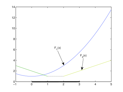
Figure 1. Pareto optimal solution set [0, 1] and weakly Pareto optimal solution set [0, 2]

The design space for this problem is shown in Figure 1. According to the above two definitions about (weakly) Pareto optimal solution, we can easily get Pareto optimal solution set for this problem is $[0,1]$, and weakly Pareto optimal solution set is $[0,2]$. Note that each Pareto optimal solution is weakly Pareto optimal solution for this problem, since $[0,1]\subseteq[0,2]$, this also shows the conclusion holds in Remark 1.

Example 2.

Let $\Omega=[0,4]$, and

$$F_{1}(x)=(x-1)^{2}+2,\ F_{2}(x)=(x-2)^{2}+1,\ F_{3}(x)=\|x\|.$$

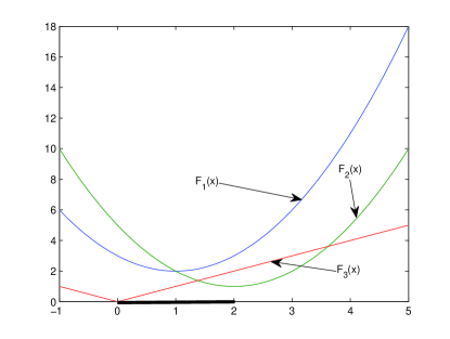
Figure 2. Pareto optimal solution set [0, 2] and weakly Pareto optimal solution set [0, 2]

For this problem, the graphs for each objective function is plotted in Figure 2. By Definitions 2.1 and 2.2, it holds that Pareto optimal solution and weakly Pareto optimal solution for this problem are the same, they all equal to $[0,2]$.

2.2. The linear weighted sum method

One useful way of getting the efficiency of problem (MOQP) is to build a utility function [17] according to the decision makers provided preference information, such that each solution gained by this method is Pareto optimal solution of problem (MOQP).

The linear weighted function

$$u(F(\cdot)):=\sum\limits_{i=1}^{p}\lambda_{i}F_{i}(\cdot)$$ (1)

is one of the most widely used utility function, where weight $\lambda_{i}$ corresponding to objective functions $F_{i}(\cdot),\ i=1,\ldots,p$ satisfy the following conditions

$$\sum\limits_{i=1}^{p}\lambda_{i}=1,\ \lambda_{i}\geq 0,\ i=1,\ldots,p,$$ (2)

which is provided by the decision makers, and weights $\lambda_{i}$ imply that the relative importance for $F_{i}(\cdot)$ in the heart of the decision makers.

3. Optimality conditions

In this section, we derive a single objective quadratic programming (SOQP) problem corresponding to problem (MOQP) by the linear weighted sum method. And, some optimality conditions for problem (MOQP) are proposed based on the optimal solutions for problem (SOQP).

From (1) and (2), problem (MOQP) can be convert to a single objective quadratic programming problem as follows

$$\rm{(SOQP)}\begin{array}[]{llll}&\min&\sum\limits_{i=1}^{p}\lambda_{i}(x^{T}Q_{i}x+2c_{i}^{T}x)&\\ &{\rm s.t.}&Ax=b,\\ &&x\geq 0.&\\ \end{array}$$

Similar to Corollary 3.1 in [17], we can get the following theorem, its proof can be found in [17].

Theorem 3.1.

Let $x^{*}$ be an optimal solution for problem (SOQP), it follows that $x^{*}$ is a Pareto optimal solution (weakly Pareto optimal solution) for problem (MOQP) if weight $\lambda>0$ ($\lambda\geq 0$, $\lambda\neq 0$).

According to the above Theorem 3.1, varying weight $\lambda$ consistently and continuously can result in a subset of Pareto optimal (weakly Pareto optimal) set for problem (MOQP). The following theorem presents a sufficient optimality condition for weakly Pareto solution of problem (MOQP).

Firstly, we quote the following definition which will be used in the sequel.

Definition 3.2.

Let $\bar{x}\in\Omega$ and $Y=F(\Omega)$, if there exists a convex set $H$ such that

$$Y\subseteq H,\ {\rm{and}}\ H\cap(F(\bar{x})-R^{p}_{++})=\emptyset,$$

then we say that $Y$ satisfies the convex inclusion condition at $F(\bar{x})$.

Based on the above convex inclusion condition, we have the following theorem. The proof is omitted here for the reason that it is similar to the one of Theorem 3.6 in [17].

Theorem 3.3.

Let $x^{*}$ be a weakly Pareto optimal solution for problem (MOQP), and $Y$ satisfies the convex inclusion condition at $F(x^{*})$. Then there exists a weight $\bar{\lambda}\geq 0,\ \bar{\lambda}\neq 0$ such that $x^{*}$ is an optimal solution for problem (SOQP) with $\bar{\lambda}$.

In particular, if problem (MOQP) is convex, Theorem 3.3 still holds without the convex inclusion condition.

4. Reformulation

Note that problem (SOQP) is a nonconvex quadratic programming problem in general, and thus it is NP-hard. If problem (SOQP) is convex with appropriate coefficient $\lambda$, we may use some popular convex packages to solve it directly. In the following section, we will establish the computable convex reformulation for problem (SOQP) when it is nonconvex, and the details are as follows.

4.1. Completely positive reformulation

Motivated by the ideas in [6], problem (SOQP) can be reformulated as a completely positive programming problem. First, the definition of completely positive [3] is given as follows.

Definition 4.1.

A symmetric matrix $B$ of order $n$ is called completely positive if one can find an integer $m$ and a matrix $V$ of size $n\times m$ with nonnegative entries such that $B=VV^{T}$, where the smallest possible number $m$ is called the CP-rank of $B$.

Based on above definition for completely positive, by using the techniques in [6], problem (SOQP) can be reformulated as the following completely positive programming problem

$$\rm{(CP)}\begin{array}[]{llll}&\min&\sum\limits_{i=1}^{p}\lambda_{i}(Q_{i}\bullet X+2c_{i}^{T}x)\\ &{\rm s.t.}&Ax=b,\\ &&{\rm{diag}}(AXA^{T})=b\circ b,\\ &&\left(\begin{array}[]{lll}1&x^{T}\\ x&X\end{array}\right)\in C_{1+n}^{*},\end{array}$$

which is a convex programming problem. Similar to Theorem 2.6 in [6], the following theorem holds immediately, for more details can be seen in [6].

Theorem 4.2.

$\it{Opt}(SOQP)=\it{Opt}(CP)$, and if $(x^{*},X^{*})$ is an optimal solution for problem (CP), then $x^{*}$ is in the convex hull of optimal solutions of problem (SOQP).

According to Theorem 4.2, problem (SOQP) is equivalent to problem (CP). However, problem (CP) is NP-hard, since there is a cone $C^{*}_{1+n}$ constraint, and check whether or not a given matrix belong to $C^{*}_{1+n}$ is shown to be NP-hard [10], one must relax it in practice. Relaxing problem (CP) in a natural way yields a doubly nonnegative programming (DNNP) problem.

4.2. Doubly nonnegative relaxation

As mentioned above, in order to establish the doubly nonnegative relaxation for problem (CP), the definition of doubly nonnegative is given as follows.

Definition 4.3.

If matrix $Z\in S_{n}$ is not only nonnegative but also positive semidefinite, then $Z$ is called doubly nonnegative.

Note that if $Z\in C^{*}_{n}$, it necessarily holds that $Z$ is doubly nonnegative from the above Definitions 4.1 and 4.3. Moreover, the convex cone $S_{n}^{+}$ is self-dual, and so is the convex cone $(S_{n})^{+}$. Hence, Diananda’s decomposition theorem [9] can be reformulated as follows.

Theorem 4.4.

For all $n$, we have $C_{n}^{*}\subseteq S_{n}^{+}\cap(S_{n})^{+}$. The relationship $"\supseteq"$ for two sets holds if and only if $n\leq 4$.

Regardless of the dimension $n$, one always has the inclusion $C_{n}^{*}\subseteq S_{n}^{+}\cap(S_{n})^{+}$. Of course, in dimension $n\geq 5$ there are matrices which are doubly nonnegative but not completely positive. The counterexample

$$M=\left[\begin{array}[]{lllllll}1&1&0&0&1\\ 1&2&1&0&0\\ 0&1&2&1&0\\ 0&0&1&2&1\\ 1&0&0&1&6\end{array}\right]$$

proposed by Diananda [9] to illustrates this point.

Replacing $C^{*}_{1+n}$ by $S_{1+n}^{+}\cap(S_{1+n})^{+}$ according to Theorem 4.4, problem (CP) is relaxed to the following doubly nonnegative programming problem

$$\rm{(DNNP)}\begin{array}[]{llll}&\min&\sum\limits_{i=1}^{p}\lambda_{i}(Q_{i}\bullet X+2c_{i}^{T}x)\\ &{\rm s.t.}&Ax=b,\\ &&{\rm{diag}}(AXA^{T})=b\circ b,\\ &&\left(\begin{array}[]{lll}1&x^{T}\\ x&X\end{array}\right)\in S_{1+n}^{+}\cap(S_{1+n})^{+},\end{array}$$

which is not only a convex problem but also can be solved in polynomial time to any fixed precision from the theory of interior-point methods.

Up to now, problem (MOQP) is reformulated as above problem (DNNP), which can be solved by some popular package CVX. It is obviously that problem (DNNP) is a relaxation form for problem (MOQP).

In the last of this section, we will investigate the relationship between optimal solutions for problems (MOQP) and (DNNP), i.e., a sufficient condition for (weakly) Pareto optimal solutions of problem (MOQP) based on the characteristics of optimal solutions for problem (DNNP) is established in the following part.

Theorem 4.5.

Let $(x^{*},X^{*})$ be an optimal solution for problem (DNNP). If the relationship $X^{*}=x^{*}(x^{*})^{T}$ holds, then ${\it{Opt(DNNP)}}={\it{Opt(CP)}}.$ Moreover, $(x^{*},X^{*})$ is an optimal solution for problem (CP).

Proof.

On one hand, from Theorem 4.4, it is obviously holds that

$${\rm{Opt}(CP)}\geq{\rm{Opt}(DNNP)}.$$ (3)

On the other hand, from $X^{*}=x^{*}(x^{*})^{T}$, and constraints of problem (CP), we have $(x^{*},X^{*})$ is also a feasible solution for problem (CP). Since problems (DNNP) and (CP) have the same objective function, it follows that

$${\rm{Opt(CP)}}\leq\sum\limits_{i=1}^{p}\lambda_{i}(Q_{i}\bullet X^{*}+2c_{i}^{T}x^{*})={\rm{Opt(DNNP)}}.$$ (4)

Thus, combining (3) and (4), we have

$${\rm{Opt(CP)}}={\rm{Opt(DNNP)}}.$$

Again from problems (CP) and (DNNP) have the same objective function, it holds that $(x^{*},X^{*})$ is an optimal solution for problem (CP). ∎

Remark 2.

It holds that ${\it{Opt(SOQP)}}={\it{Opt(CP)}}$ from Theorem 4.2. Let $(x^{*},X^{*})$ be an optimal solution for problem (DNNP), if $X^{*}=x^{*}(x^{*})^{T}$, by Theorem 4.5, we have ${\it{Opt(CP)}}={\it{Opt(DNNP)}}.$ Thus, we get ${\it{Opt(SOQP)}}={\it{Opt(DNNP)}}$ under the condition $X^{*}=x^{*}(x^{*})^{T}$. Furthermore, since problems (SOQP) and (DNNP) have the same objective function, again from Theorem 4.2, we can conclude that $x^{*}$ is an optimal solution for problem (SOQP). From Theorem 3.1, we further know that $x^{*}$ is a Pareto optimal solution (or weakly Pareto optimal solution) for problem (MOQP) if $\lambda>0$ (or $\lambda\geq 0$).

5. Numerical experiments

In this section, in order to show the effectiveness of our proposed method, some examples are tested and corresponding numerical results are reported. To solve test problems, we use CVX [11], a package for specifying and solving convex programs. The software is implemented using MATLAB R2011b on Windows 7 platform, and on a PC with Intel(R) Core(TM) i3-2310M CPU 2.10 GHz.

In the following numerical experiments, three examples are solved by using the proposed method, respectively. The first example is a given two-dimension problem, which has four nonconvex objective functions. The second example is a five-dimension nonconvex problem with five objective functions. Note that its coefficients are generated by MATLAB function randn($\cdot$). The last example is a practical portfolio selection problem, which is taken from [16]. The weighted coefficient $\lambda$ is generated by the following procedure

lambda=zeros(p,1);

while lambda(p)==0

lambda(1:p-1)=rand(p-1,1); s=sum(lambda);

if s<1 lambda(p)=1-s; end

end
where $p$ is the number of objective functions.

Example 3.

First of all, a two-dimension problem with four objective functions is tested. The corresponding coefficients $Q_{i},\ c_{i},\ i=1,\ldots,4$ and $A,\ b$ are given in Table 1.

Table 1. Coefficients for Example 3

$Q_{1}=\left[\begin{array}[]{ll}1&3\\ 3&8\end{array}\right]$	$Q_{2}=\left[\begin{array}[]{lllll}2&0\\ 0&-2\end{array}\right]$	$Q_{3}=\left[\begin{array}[]{lllll}0&2\\ 2&0\end{array}\right]$	$Q_{4}=\left[\begin{array}[]{llllll}-1&0\\ 0&0\end{array}\right]$
$c_{1}=[2.5\ \ -0.5]^{T}$	$c_{2}=[-1\ \ -1.5]^{T}$	$c_{3}=[1\ \ 0.5]^{T}$	$c_{4}=[1\ \ 1.5]^{T}$
$A=[1\ \ 1]$	$b=1$

First, by relative simple computation, we obtain optimal solutions for each objective function which is minimized independently. The corresponding optimal numerical results of each objective function are given in Table 2.

Table 2. Optimal numerical results for each objective function of Example 3

	$F_{1}(x^{*})$					$F_{2}(x^{*}$)					$F_{3}(x^{*}$)					$F_{4}(x^{*}$)
FV	$5.6667$					$-5$					$1$					$1$
$x^{*}$	$(0.6667\ 0.3333)^{T}$					$(0\ 1)^{T}$					$(0\ 1)^{T}$					$(1\ 0)^{T}$

In Table 2, the labels FV and $x^{*}$ denotes optimal values and optimal solutions corresponding to each objective function, respectively. The results in Table 2 show that the objective functions $F_{2}(x)$ and $F_{3}(x)$ have the same optimal solution, which is different from the other two functions optimal solutions. These imply that we can not find a single solution that simultaneously optimizes each objective function. Moreover, note that these four optimal solutions corresponding to each objective function are all weakly Pareto optimal solutions for Example 3.

Table 3. Optimal numerical results for Example 3 in (DNNP)

$\lambda$	FV	$x^{*}$	$X^{*}$
$(0.5472\ 0.1386\ 0.1493\ 0.1649)$	$\left[\begin{array}[]{ll}5.8345\\ -2.8494\\ 2.4106\\ 2.3849\end{array}\right]$	$\left[\begin{array}[]{ll}0.4301\\ 0.5699\end{array}\right]$	$\left[\begin{array}[]{ll}0.1850&0.2451\\ 0.2451&0.3248\end{array}\right]$
$(0.3500\ 0.1966\ 0.2511\ 0.2023)$	$\left[\begin{array}[]{ll}7.0000\\ -5.0000\\ 1.0000\\ 3.0000\end{array}\right]$	$\left[\begin{array}[]{ll}0.0000\\ 1.0000\end{array}\right]$	$\left[\begin{array}[]{ll}0.0000&0.0000\\ 0.0000&1.0000\end{array}\right]$
$(0.0759\ 0.0540\ 0.5308\ 0.3394)$	$\left[\begin{array}[]{ll}6.0000\\ 0.0000\\ 2.0000\\ 1.0000\end{array}\right]$	$\left[\begin{array}[]{ll}1.0000\\ 0.0000\end{array}\right]$	$\left[\begin{array}[]{ll}1.0000&0.0000\\ 0.0000&0.0000\end{array}\right]$
$(0.2417\ 0.4039\ 0.0965\ 0.2579)$	$\left[\begin{array}[]{ll}5.6670\\ -1.6105\\ 2.5513\\ 1.8625\end{array}\right]$	$\left[\begin{array}[]{ll}0.6779\\ 0.3221\end{array}\right]$	$\left[\begin{array}[]{ll}0.4596&0.2183\\ 0.2183&0.1037\end{array}\right]$
$(0.5752\ 0.0598\ 0.2348\ 0.1302)$	$\left[\begin{array}[]{ll}5.8570\\ -2.9261\\ 2.3857\\ 2.4132\end{array}\right]$	$\left[\begin{array}[]{ll}0.4148\\ 0.5852\end{array}\right]$	$\left[\begin{array}[]{ll}0.1720&0.2427\\ 0.2427&0.3425\end{array}\right]$
$(0.0430\ 0.1690\ 0.6491\ 0.1389)$	$\left[\begin{array}[]{ll}7.0000\\ -5.0000\\ 1.0000\\ 3.0000\end{array}\right]$	$\left[\begin{array}[]{ll}0.0000\\ 1.0000\end{array}\right]$	$\left[\begin{array}[]{ll}0.0000&0.0000\\ 0.0000&1.0000\end{array}\right]$
$(0.2259\ 0.1707\ 0.2277\ 0.3757)$	$\left[\begin{array}[]{ll}6.0000\\ 0.0000\\ 2.0000\\ 1.0000\end{array}\right]$	$\left[\begin{array}[]{ll}1.0000\\ 0.0000\end{array}\right]$	$\left[\begin{array}[]{ll}1.0000&0.0000\\ 0.0000&0.0000\end{array}\right]$
$(0.2920\ 0.4317\ 0.0155\ 0.2609)$	$\left[\begin{array}[]{ll}5.7480\\ -2.4901\\ 2.5020\\ 2.2460\end{array}\right]$	$\left[\begin{array}[]{ll}0.5020\\ 0.4980\end{array}\right]$	$\left[\begin{array}[]{ll}0.2520&0.2500\\ 0.2500&0.2480\end{array}\right]$
$(0.2607\ 0.5944\ 0.0225\ 0.1224)$	$\left[\begin{array}[]{ll}5.7480\\ -2.4901\\ 2.5020\\ 2.2460\end{array}\right]$	$\left[\begin{array}[]{ll}0.5020\\ 0.4980\end{array}\right]$	$\left[\begin{array}[]{ll}0.2520&0.2500\\ 0.2500&0.2480\end{array}\right]$

It is very easy to verify that the given four objective functions are all nonconvex by using MATLAB function eig. Furthermore, we obtain problem (SOQP) is nonconvex with corresponding coefficients $\lambda$ which proposed in Table 3 by using eig. Hence, we use our method to solve this problem. The corresponding optimal numerical results are reported in Table 3. In Table 3, Example 3 is transformed into problem (DNNP), and then is solved with nine different weighted coefficient $\lambda$. The results of $x^{*}$ and $X^{*}$ in Table 3 show that $X^{*}=x^{*}(x^{*})^{T}$ holds for nine different weighted coefficients. Thus, from Theorem 4.5 and Remark 2, it holds that each optimal solution $x^{*}$ in Table 3 also is Pareto optimal solution for Example 3. Moreover, we obtain weakly Pareto optimal solutions for Example 3 when the weighted coefficient $\lambda$ is chosen appropriately. For instance, if $\lambda$ is chosen as $(0.3500,0.1966,0.2511,0.2023)$ or $(0.0430,0.1690,0.6491,0.1389)$, then weakly Pareto optimal solution $(0.0000,1.0000)^{T}$ is obtained by using our method.

Example 4.

In this test problem, we set $n=5$, $m=4$ and $p=5$. The corresponding coefficients $Q_{i},\ c_{i},\ i=1,\ldots,5$ and $A,\ b$ are generated by the functions tril(randn(n,n),-1)+triu(randn(n,n)’,0), randn(n,1), randn(n,m) and
randn(m,1), respectively, and the details can be seen in Table 4.

Table 4. Coefficients for Example 4

$Q_{1}=\left[\begin{array}[]{lllllll}0.4056&-1.4193&-0.7294&1.1473&0.5979\\ -1.4193&-2.2033&-0.5712&0.2140&0.9424\\ -0.7294&-0.5712&0.3062&-1.1723&-0.9610\\ 1.1473&0.2140&-1.1723&-0.9000&-0.2857\\ 0.5979&0.9424&-0.9610&-0.2857&0.6103\end{array}\right]$	$c_{1}=\left[\begin{array}[]{ll}0.7907\\ 0.2877\\ 0.0032\\ 0.3656\\ 3.5267\end{array}\right]$
$Q_{2}=\left[\begin{array}[]{lllll}0.0591&-1.4669&-1.6258&-1.9648&2.6052\\ -1.4669&0.2570&-0.9742&-1.1464&0.5476\\ -1.6258&-0.9742&-0.4494&-0.0843&-1.9920\\ -1.9648&-1.1464&-0.0843&-0.3909&0.4092\\ 2.6052&0.5476&-1.9920&0.4092&1.3018\end{array}\right]$	$c_{2}=\left[\begin{array}[]{ll}-0.1124\\ -1.5566\\ 1.9151\\ 0.6098\\ -0.6479\end{array}\right]$
$Q_{3}=\left[\begin{array}[]{lllll}-0.5936&0.4364&-0.5044&0.1021&1.1963\\ 0.4364&-1.0368&-0.8571&-0.1699&-0.1917\\ -0.5044&-0.8571&1.2665&-0.2512&-0.2046\\ 0.1021&-0.1699&-0.2512&-0.3862&0.5256\\ 1.1963&-0.1917&-0.2046&0.5256&0.8175\end{array}\right]$	$c_{3}=\left[\begin{array}[]{ll}2.6173\\ 0.5510\\ 0.2942\\ -0.7778\\ -1.0649\end{array}\right]$
$Q_{4}=\left[\begin{array}[]{llllll}0.4902&0.7653&0.7783&-1.4803&0.5404\\ 0.7653&-0.7603&-0.6936&1.2815&-0.8097\\ 0.7783&-0.6936&2.0108&0.0256&0.3083\\ -1.4803&1.2815&0.0256&0.5301&-0.9521\\ 0.5404&-0.8097&0.3083&-0.9521&-0.4506\end{array}\right]$	$c_{4}=\left[\begin{array}[]{ll}-1.7684\\ -0.4229\\ -1.0531\\ 0.6478\\ -0.3176\end{array}\right]$
$Q_{5}=\left[\begin{array}[]{lllllll}0.1092&-0.2506&-0.1899&-1.0329&-0.3233\\ -0.2506&1.7447&-1.1605&2.3774&1.5261\\ -0.1899&-1.1605&-0.6987&0.8328&-0.6946\\ -1.0329&2.3774&0.8328&0.8967&0.5047\\ -0.3233&1.5261&-0.6946&0.5047&1.1867\end{array}\right]$	$c_{5}=\left[\begin{array}[]{ll}1.7690\\ 1.5106\\ 0.1640\\ -0.2828\\ 1.1522\end{array}\right]$
$A=\left[\begin{array}[]{llllll}-1.1465&-0.6718&0.5530&0.2695&1.0393\\ 0.6737&0.5756&-0.4234&-2.5644&0.9109\\ -0.6691&-0.7781&0.3616&0.4659&-0.2397\\ -0.4003&-1.0636&-0.3519&1.8536&0.1810\end{array}\right]$	$b=\left[\begin{array}[]{ll}0.2442\\ 0.0964\\ -0.8305\\ -0.3523\end{array}\right]$

In order to verify that whether the given objective functions in Table 4 are nonconvex functions or not, the corresponding eigenvalues for $Q_{i},\ i=1,\ldots,5$ are given in Table 5. The results in Table 5 show that five objective functions are all nonconvex. Thus, we will use the proposed method to solve this problem. The results are given in Tables 6 and 7.

Table 5. Eigenvalues for $Q_{i},\ i=1,\ldots,5$ in Example 4

Quadratic matrices	Eigenvalues
$Q_{1}$	$(-3.3892,-1.8503,-0.0780,1.1180,2.4184)$
$Q_{2}$	$(-4.2248,-1.8386,0.7234,1.3339,4.7837)$
$Q_{3}$	$(-1.6777,-1.1336,-0.3917,1.1973,2.0731)$
$Q_{4}$	$(-2.5335,-1.0738,0.6848,1.6750,3.0677)$
$Q_{5}$	$(-2.3512,-0.6382,0.1606,1.3837,4.6838)$

Table 6. Optimal numerical results for each objective function of Example 4

					FV					$x^{*}$
$F_{1}(x^{*})$					$2.1900$					$(0,\ 1.2165,\ 0.2253,\ 0.4747,\ 0.7783)^{T}$
$F_{2}(x^{*})$					$-9.2542$					$(2.7216,\ 0,\ 2.7773,\ 0.7727,\ 1.5592)^{T}$
$F_{3}(x^{*})$					$-1.3755$					$(0,\ 1.2165,\ 0.2253,\ 0.4747,\ 0.7783)^{T}$
$F_{4}(x^{*})$					$-2.2276$					$(0.4915,\ 0.9969,\ 0.6861,\ 0.5285,\ 0.9193)^{T}$
$F_{5}(x^{*})$					$0.6759$					$(2.7216,\ 0,,\ 2.7773,\ 0.7727,\ 1.5592)^{T}$

Table 6 shows that the optimal numerical results for each objective function of Example 4. The results in Table 6 show that we can not find a single solution that simultaneously optimizes these five objective functions. Note that these five optimal solutions are also weakly Pareto optimal solutions for Example 4.

Table 7. Optimal numerical results for Example 4 in (DNNP)

$\lambda$	FV	$x^{*}$	$X^{*}$
$\left[\begin{array}[]{ll}0.3317\\ 0.1522\\ 0.3480\\ 0.1217\\ 0.0464\end{array}\right]$	$\left[\begin{array}[]{llllll}2.1900\\ -1.7656\\ -1.3755\\ -1.7914\\ 7.0248\end{array}\right]$	$\left[\begin{array}[]{ll}0.0000\\ 1.2165\\ 0.2253\\ 0.4747\\ 0.7783\end{array}\right]$	$\left[\begin{array}[]{lllll}0.0000&0.0000&0.0000&0.0000&0.0000\\ 0.0000&1.4799&0.2741&0.5775&0.9469\\ 0.0000&0.2741&0.0508&0.1070&0.1753\\ 0.0000&0.5775&0.1070&0.2254&0.3695\\ 0.0000&0.9469&0.1753&0.3695&0.6058\end{array}\right]$
$\left[\begin{array}[]{ll}0.0712\\ 0.1820\\ 0.0930\\ 0.4635\\ 0.1903\end{array}\right]$	$\left[\begin{array}[]{lll}2.2944\\ -2.3834\\ 0.1927\\ -2.2196\\ 6.2356\end{array}\right]$	$\left[\begin{array}[]{ll}0.4250\\ 1.0266\\ 0.6238\\ 0.5213\\ 0.9003\end{array}\right]$	$\left[\begin{array}[]{lllllll}0.1806&0.4363&0.2651&0.2215&0.3826\\ 0.4363&1.0538&0.6403&0.5351&0.9242\\ 0.2651&0.6403&0.3891&0.3252&0.5616\\ 0.2215&0.5351&0.3252&0.2717&0.4693\\ 0.3826&0.9242&0.5616&0.4693&0.8105\end{array}\right]$
$\left[\begin{array}[]{ll}0.0290\\ 0.6371\\ 0.0595\\ 0.1692\\ 0.1052\end{array}\right]$	$\left[\begin{array}[]{ll}2.3045\\ -2.4426\\ 0.3234\\ -2.2257\\ 6.1681\end{array}\right]$	$\left[\begin{array}[]{ll}0.4595\\ 1.0111\\ 0.6562\\ 0.5251\\ 0.9102\end{array}\right]$	$\left[\begin{array}[]{llllll}0.2111&0.4646&0.3015&0.2413&0.4182\\ 0.4646&1.0224&0.6635&0.5309&0.9203\\ 0.3015&0.6635&0.4305&0.3445&0.5972\\ 0.2413&0.5309&0.3445&0.2757&0.4779\\ 0.4182&0.9203&0.5972&0.4779&0.8284\end{array}\right]$
$\left[\begin{array}[]{ll}0.0472\\ 0.0559\\ 0.0715\\ 0.0157\\ 0.8098\end{array}\right]$	$\left[\begin{array}[]{ll}3.5136\\ -9.2542\\ 9.9301\\ 6.7545\\ 0.6759\end{array}\right]$	$\left[\begin{array}[]{ll}2.7216\\ 0.0000\\ 2.7773\\ 0.7727\\ 1.5592\end{array}\right]$	$\left[\begin{array}[]{llllll}7.4071&0.0000&7.5586&2.1030&4.2434\\ 0.0000&0.0000&0.0000&0.0000&0.0000\\ 7.5586&0.0000&7.7132&2.1460&4.3302\\ 2.1030&0.0000&2.1460&0.5971&1.2048\\ 4.2434&0.0000&4.3302&1.2048&2.4310\end{array}\right]$
$\left[\begin{array}[]{ll}0.1911\\ 0.0504\\ 0.5484\\ 0.0095\\ 0.2006\end{array}\right]$	$\left[\begin{array}[]{ll}2.1900\\ -1.7656\\ -1.3755\\ -1.7914\\ 7.0248\end{array}\right]$	$\left[\begin{array}[]{ll}0.0000\\ 1.2165\\ 0.2253\\ 0.4747\\ 0.7783\end{array}\right]$	$\left[\begin{array}[]{lllll}0.0000&0.0000&0.0000&0.0000&0.0000\\ 0.0000&1.4799&0.2741&0.5775&0.9469\\ 0.0000&0.2741&0.0508&0.1070&0.1753\\ 0.0000&0.5775&0.1070&0.2254&0.3695\\ 0.0000&0.9469&0.1753&0.3695&0.6058\end{array}\right]$
$\left[\begin{array}[]{ll}0.2166\\ 0.6291\\ 0.0149\\ 0.0433\\ 0.0961\end{array}\right]$	$\left[\begin{array}[]{ll}3.5136\\ -9.2542\\ 9.9301\\ 6.7545\\ 0.6759\end{array}\right]$	$\left[\begin{array}[]{ll}2.7216\\ 0.0000\\ 2.7773\\ 0.7727\\ 1.5592\end{array}\right]$	$\left[\begin{array}[]{lllll}7.4071&0.0000&7.5586&2.1030&4.2434\\ 0.0000&0.0000&0.0000&0.0000&0.0000\\ 7.5586&0.0000&7.7132&2.1460&4.3302\\ 2.1030&0.0000&2.1460&0.5971&1.2048\\ 4.2434&0.0000&4.3302&1.2048&2.4310\end{array}\right]$
$\left[\begin{array}[]{ll}0.2583\\ 0.0041\\ 0.0905\\ 0.5958\\ 0.0513\end{array}\right]$	$\left[\begin{array}[]{ll}2.2080\\ -1.8738\\ -1.0651\\ -1.9303\\ 6.8716\end{array}\right]$	$\left[\begin{array}[]{ll}0.0857\\ 1.1782\\ 0.3057\\ 0.4841\\ 0.8029\end{array}\right]$	$\left[\begin{array}[]{lllll}0.0073&0.1010&0.0262&0.0415&0.0688\\ 0.1010&1.3882&0.3601&0.5704&0.9460\\ 0.0262&0.3601&0.0934&0.1480&0.2454\\ 0.0415&0.5704&0.1480&0.2344&0.3887\\ 0.0688&0.9460&0.2454&0.3887&0.6447\end{array}\right]$

Note that we can verify that problem (SOQP) is nonconvex with seven different choices of weighted coefficient $\lambda$ which show in Table 7. So, Example 4 can be solved by using the proposed method. The results of $x^{*}$ and $X^{*}$ in Table 7 show that $X^{*}=x^{*}(x^{*})^{T}$ holds for these seven different cases of weighted coefficient $\lambda$. Hence, we can conclude that each $x^{*}$ in Table 7 also is Pareto optimal solution for Example 4. Furthermore, compare the results of FV and $x^{*}$ in Tables 6 and 7, note that some weakly Pareto optimal solutions of Example 4 can be obtained by using our method. For example, if $\lambda=(0.3317,0.1522,0.3480,0.1217,0.0464)$, then we obtain weakly Pareto optimal solution $(0.0000,1.2165,0.2253,0.4747,0.7783)^{T}$ for Example 4.

Remark 3.

The results for Example 3 and Example 4 imply that we not only obtain Pareto optimal solutions, but also obtain some weakly Pareto optimal solutions for original problem with appropriate choices of weighted coefficient $\lambda$. Summarizing these results, we can conclude that our method is effective for solving some problems (MOQP).

Example 5.

(Portfolio Selection Problem) This problem is taken from [16]. It is a practical portfolio selection problem in which objective function $F(x)$ has the following expression

$$F(x)=(\frac{1}{2}x^{T}Q_{1}x,\ -c_{2}^{T}x,\ -c_{3}^{T}x)^{T},$$

where symmetric matrix $Q_{1}$ is called the risk matrix, $c_{2}$ denotes the return rate vector, $c_{3}$ is a given weighting vector and its element is a function of corresponding security liquidity. The corresponding coefficients are given in Table 8.

Table 8. Coefficients for Example 5

$Q_{1}=\left[\begin{array}[]{llllllllllllllllllllll}12.35&-8.64&9.88&-8.43&9.42&-1.47&4.29&-0.96&15.2&0\\ -8.64&6.42&-8.15&5.13&4.56&5.83&-6.72&0.78&3.42&0\\ 9.88&-8.15&18.27&-8.14&2.32&-4.12&-1.85&1.34&0.795&0\\ -8.43&5.13&-8.14&12.6&-8.43&7.47&-4.67&-0.679&8.09&0\\ 9.42&4.56&2.32&-8.43&17.07&7.33&-3.18&-0.547&0.323&0\\ -1.47&5.83&-4.12&7.47&7.33&13.38&-3.84&-0.478&0.616&0\\ 4.29&-6.27&-1.85&-4.67&-3.18&-3.84&3.41&0.107&0.464&0\\ -0.96&-0.78&1.34&-0.679&-0.547&-0.478&0.107&1.33&11.23&0\\ 15.2&3.42&0.795&0.809&0.323&0.616&0.464&11.23&2.45&0\\ 0&0&0&0&0&0&0&0&0&0\end{array}\right]$

$c_{2}=[11.11\ \ 17.78\ \ 2.22\ \ 18.28\ \ 12.6\ \ 10.15\ \ 6.72\ \ 5.75\ \ 6.1\ \ 2.25]^{T}$

$c_{3}=[0.069\ \ 0.092\ \ 0.046\ \ 0.096\ \ 0.086\ \ 0.068\ \ 0.06\ \ 0.145\ \ 0.151\ \ 0.197]^{T}$

$A=[1\ 1\ 1\ 1\ 1\ 1\ 1\ 1\ 1\ 1]\ \ \ b=1$

Note that the objective functions contain only one quadratic function $\frac{1}{2}x^{T}Q_{1}x$, by using eig function of MATLAB, it is easy to verify that function $\frac{1}{2}x^{T}Q_{1}x$ is nonconvex. Thus, we use the proposed method to solve this problem. The corresponding optimal results are given in Table 9.

Table 9. Optimal numerical results for Example 5

$\lambda$	FV	$x^{*}$
$\left[\begin{array}[]{ll}0.3482\\ 0.1655\\ 0.4863\end{array}\right]$	$\left[\begin{array}[]{ll}0.1894\\ -15.6800\\ -0.0850\end{array}\right]$	$(0.3240,0.5567,0.0000,0.1194,0.0000,0.0000,0.0000,0.0000,0.0000,0.0000)^{T}$
$\left[\begin{array}[]{ll}0.5141\\ 0.1931\\ 0.2927\end{array}\right]$	$\left[\begin{array}[]{ll}0.1320\\ -15.5462\\ -0.0846\end{array}\right]$	$(0.3433,0.5466,0.0000,0.1101,0.0000,0.0000,0.0000,0.0000,0.0000,0.0000)^{T}$
$\left[\begin{array}[]{ll}0.6167\\ 0.3087\\ 0.0746\end{array}\right]$	$\left[\begin{array}[]{ll}0.2026\\ -15.7070\\ -0.0851\end{array}\right]$	$(0.3200,0.5590,0.0000,0.1210,0.0000,0.0000,0.0000,0.0000,0.0000,0.0000)^{T}$

In Table 9, Example 5 is solved with three different values of weight $\lambda$. The first element and the absolute value of the second element of FV in Table 9 denote the expectation risk and return, respectively. The results in Table 9 show that we obtain the lower risk and higher return when weight $\lambda$ is chosen appropriately. Moreover, we also compare with the results in [16], which are show in Table 10.

Table 10. Optimal numerical results for Example 5 in [16]

FV	$x^{*}$
$\left[\begin{array}[]{ll}0.6823\\ -7.5079\\ -0.1343\end{array}\right]$	$(0.0453,0.0706,0.0273,0.0703,0.078,0.045,0.0534,0.169,0.1665,0.2746)^{T}$

The results of FV in Tables 9 further imply that the risk and return are more comparable with the results in Table 10. For example, when $\lambda=(0.3482,0.1655,0.4863)$, we obtain lower risk $0.1894$ and higher return $15.6800$, which are more comparable with the results of [16] $0.6823$ and $7.5079$, respectively. Furthermore, note that the optimal solutions $x^{*}$ obtained by using our method are sparse, which imply that we mainly focus on some kinds of important stocks. Hence, we can put together the limited money, and invest these money in some of important stocks to obtain more satisfied return with lower risk.

We also notice that there are infinite choices of weight $\lambda$, and not all choices of weight $\lambda$ are reasonable for each investor. How to select weight $\lambda$ to lower risk and higher return depends on the investors’s preference. Therefore, it is reasonable that investors participate in decision making and continuously revise their preferences according to practical conditions. This also shows that our method is promising in solving portfolio selection problems.

6. Concluding remarks

In this paper, a class of (MOQP) problems is discussed. By using the linear weighted sum method to deal with quadratic objective functions, problem (MOQP) is transformed into problem (SOQP), which is nonconvex in general. Then, taking advantage of lifting techniques, problem (SOQP) is equivalently reformulated as problem (CP) which is a convex programming problem but NP-hard in general. A computable relaxed convex problem (DNNP) for problem (CP) is obtained by using doubly nonnegative relaxation method. Moreover, based on the characteristics of optimal solutions for problem (DNNP), a sufficient condition for (weakly) Pareto optimal solutions for problem (MOQP) is proposed. Finally, the numerical results of two problems and a practical portfolio selection problem show that the proposed method is effective and promising.

Received xxxx 20xx; revised xxxx 20xx.

References

• [1] (MR2363231) E.E. Ammar, On solutions of fuzzy random multiobjective quadratic programming with applications in portfolio problem, Information Sciences, 178 (2008), no. 2, 468–484.
• [2] (MR2463270) E.E. Ammar, On fuzzy random multiobjective quadratic programming, European Journal of Operational Research, 193 (2009), no. 2, 329–341.
• [3] (MR1986666) A. Berman and N. Shaked-Monderer, “Completely positive matrices,” World Scientific Publishing Co. Inc., River Edge, NJ, 2003.
• [4] (MR2845851) Immanuel M. Bomze, Copositive optimization—recent developments and applications, European Journal of Operational Research, 216 (2012), no. 3, 509–520.
• [5] (MR2061575) S. Boyd and L. Vandenberghe, “Convex optimization,” Cambridge University Press, Cambridge, 2004.
• [6] (MR2505747) S. Burer, On the copositive representation of binary and continuous nonconvex quadratic programs, Mathematical Programming, Ser. A, 210 (2009), no. 2, 479–495.
• [7] (MR2601718) S. Burer, Optimizing a polyhedral-semidefinite relaxation of completely positive programs, Mathematical Programming Computation, 2 (2010), no. 1, 1–19.
• [8] O. Dandekar, W. Plishker, S. Bhattacharyya and R. Shekhar, Multi-objective optimization for reconfigurable implementation of medical image registration, International Journal of Reconfigurable Computing, 2008 (2009), 1–17.
• [9] (MR0137686) P.H. Diananda, On non-negative forms in real variables some or all of which are non-negative, in “Mathematical Proceedings of the Cambridge Philosophical Society”, Cambridge University Press, 58 (1962), no. 1, 17–25.
• [10] P. Dickinson and L. Gijben, “On the computational complexity of mem- bership problems for the completely positive cone and its dual,” Technical Report, Johann Bernoulli Institute for Mathematics and Computer Science, University of Groningen, The Netherlands, 2011.
• [11] M. Grant and S. Boyd, CVX: Matlab software for disciplined convex programming, version 1.21, April, 2011. Available from: http://cvxr.com/cvx.
• [12] Y. Hu, “Efficiency theory of multiobjective programming,” Shanghai Scientific and Technical Publishers, 1994.
• [13] P. Korhonen and G.Y. Yu, A reference direction approach to multiple objective quadratic-linear programming, European Journal of Operational Research, 102 (1997), no. 3, 601–610.
• [14] (MR2869505) C. Lu, S.C. Fang, Q.W. Jin, Qingwei, Z.B. Wang and W.X. Xing, KKT solution and conic relaxation for solving quadratically constrained quadratic programming problems, SIAM Journal on Optimization, 21 (2011), no. 4, 1475–1490.
• [15] (MR2610844) R.T. Marler and J.S. Arora, The weighted sum method for multi-objective optimization: new insights, Structural and multidisciplinary optimization, 41 (2010), no. 6, 853–862.
• [16] (MR1923449) J.P. Xu and J. Li, A class of stochastic optimization problems with one quadratic $\&$ several linear objective functions and extended portfolio selection model, Journal of Computational and Applied Mathematics, 146 (2002), no. 1, 99–113.
• [17] J.P. Xu and J. Li, “Multiple objective decision making theory and methods,” Tsinghua University Press, 2005.
• [18] B.R. Ye and L.H. Yu, Generating noninferior set of a multi-objective quadratic programming and application, Water Resources and Power, 9 (1991), no. 2. 102–110.