Forest Sparsity for Multi-channel Compressive Sensing

Abstract

In this paper, we investigate a new compressive sensing model for multi-channel sparse data where each channel can be represented as a hierarchical tree and different channels are highly correlated. Therefore, the full data could follow the forest structure and we call this property as forest sparsity. It exploits both intra- and inter- channel correlations and enriches the family of existing model-based compressive sensing theories. The proposed theory indicates that only $\mathcal{O}(Tk+\log(N/k))$ measurements are required for multi-channel data with forest sparsity, where $T$ is the number of channels, $N$ and $k$ are the length and sparsity number of each channel respectively. This result is much better than $\mathcal{O}(Tk+T\log(N/k))$ of tree sparsity, $\mathcal{O}(Tk+k\log(N/k))$ of joint sparsity, and far better than $\mathcal{O}(Tk+Tk\log(N/k))$ of standard sparsity. In addition, we extend the forest sparsity theory to the multiple measurement vectors problem, where the measurement matrix is a block-diagonal matrix. The result shows that the required measurement bound can be the same as that for dense random measurement matrix, when the data shares equal energy in each channel. A new algorithm is developed and applied on four example applications to validate the benefit of the proposed model. Extensive experiments demonstrate the effectiveness and efficiency of the proposed theory and algorithm.

I Introduction

Sparsity techniques are becoming more and more popular in machine learning, statistics, medical imaging and computer vision as the emerging of compressive sensing. Based on compressive sensing theory [1, 2], a small number of measurements are enough to recover the original data, which is an alternative to Shannon/Nyquist sampling theorem for sparse or compressible data acquisition.

I-A Standard Sparsity and Algorithms

Suppose $A\in\mathbb{R}^{M\times N}$ is the sampling matrix and $b\in\mathbb{R}^{M}$ is the measurement vector, the problem is to recover the sparse data $x\in\mathbb{R}^{N}$ by solving the linear system $Ax=b$. Sometimes the data is not sparse but compressible under some base $\Phi$ such as wavelet, and the corresponding problem is $A\Phi^{-1}\theta=b$ where $\theta$ denotes the set of wavelet coefficients. Although the problem is underdetermined, the data can be perfectly reconstructed if the sampling matrix satisfy restricted isometry property (RIP) [3] and the number of measurements is larger than $\mathcal{O}(k+k\log(N/k))$ for $k$-sparse data [4, 5].

To solve the underdetermined problem, we may find the sparsest solution via $\ell_{0}$ norm regularization. However, because the problem is NP-hard [6] and impractical for most applications , $\ell_{1}$ norm regularization methods such as the lasso [7] and basis pursuit (BP) [8] are first used to pursue the sparse solution. It has been proved that the $\ell_{1}$ norm regularization can exactly recover the sparse data for CS inverse problem under mild conditions [9, 1]. Therefore, a lot of efficient algorithms have been proposed for standard sparse recovery. Generally speaking, those algorithms can be classified into three groups: greedy algorithms [10, 11], convex programming [12, 13, 14] and probability based methods [15, 16].

I-B Joint Sparsity and Algorithms

Beyond standard sparsity, the non-zeros components of $x$ often tend to be in some structures. This comes to the concept of structured sparsity or model-based compressive sensing [17, 18, 19]. In contrast to standard sparsity that only relies on the sparseness of the data, structured sparsity models exploit both the non-zero values and the corresponding locations. For example, in the multiple measurement vector (MMV) problem, the data is consisted of several vectors that share the same support . This is called joint sparsity that widely arise in cognitive radio networks [20], direction-of-arrival estimation in radar [21], multi-channel compressive sensing [22, 23] and medical imaging [24, 25]. If the data $X\in\mathbb{R}^{TN\times 1}$ is consist of $T$ $k$-sparse vectors, the measurement bound could be substantially reduced to $\mathcal{O}(Tk+k\log(N/q))$ instead of $\mathcal{O}(Tk+Tk\log(N/q))$ for standard sparsity [26, 17, 18, 27].

A common way to implement joint sparsity in convex programming is to replace the $\ell_{1}$ norm with $\ell_{2,1}$ norm, which is the summation of $\ell_{2}$ norms of the correlated entries [28, 29]. $\ell_{2,1}$ norm for joint sparsity has been used in many convex solvers and algorithms [30, 25, 31, 32]. In Bayesian sparse learning or approximate message passing [33, 34, 35], data from all channels contribute to the estimation of parameters or hidden variables in the sparse prior model.

I-C Tree Sparsity and Algorithms

Another common structure would be the hierarchical tree structure, which has already been successfully utilized in image compression [36], compressed imaging [37, 38, 39, 40], and machine learning [41]. Most nature signals/images are approximately tree-sparse under the wavelet basis. A typical relationship with tree sparsity is that, if a node on the tree is non-zero, all of its ancestors leading to the root should be non-zeros. For multi-channel data $X=[x_{1};x_{2},...;x_{T}]\in\mathbb{R}^{NT\times 1}$, $\mathcal{O}(Tk+T\log(N/k))$ measurements are required if each channel $x_{t}$ is tree-sparse.

Due to the overlapping and intricate structure of tree sparsity, it is much harder to implement. For greedy algorithms, StructOMP [17] and TOMP [42] are developed for exploiting tree structure where the coefficients are updated by only searching the subtree blocks instead of all subspace. In statistical models [37, 38], hierarchical inference is used to model the tree structure, where the value of a node is not independent but relies on the distribution or state of its parent. In convex programming [39, 43], due to the tradeoff between the recovery accuracy and computational complexity, this is often approximated as overlapping group sparsity [44], where each node and its parent are assigned into one group.

I-D Forest Sparsity

Although both joint sparsity and tree sparsity have been widely studied, unfortunately, there is no work that study the benefit of their combinations so far. Actually, in many multi-channel compressive sensing or MMV problems, the data has joint sparsity across different channels and each channel itself is tree-sparse. Note that this differs from C-HiLasso [45], where sparsity is assumed inside the groups. No method has fully exploited both priors and no theory guarantees the performance. In practical applications, researchers and engineers have to choose either joint sparsity algorithms by giving up their intra tree-sparse prior, or tree sparsity algorithms by ignoring their inter correlations.

In this paper, we propose a new sparsity model called forest sparsity to bridge this gap. It is a natural extension of existing structured sparsity models by assuming that the data can be represented by a forest of mutually connected trees. We give the mathematical definition of forest sparsity. Based on compressive sensing theory, we prove that for a forest of $T$ k-sparse trees, only $\mathcal{O}(Tk+\log(N/k))$ measurements are required for successful recovery with high probability. That is much less than the bounds of joint sparsity $\mathcal{O}(Tk+k\log(N/k))$ and tree sparsity $\mathcal{O}(Tk+T\log(N/k))$ on the same data. The theory is further extended to the case on MMV problems, which is ignored in existing structured sparsity theories [17, 18, 19]. Finally, we derive an efficient algorithm to optimize the forest sparsity model. The proposed algorithm is applied on medical imaging applications such as multi-contrast magnetic resonance imaging (MRI), parallel MRI (pMRI), as well as color images, multispectral image reconstruction. Extensive experiments demonstrate the advantages of forest sparsity over the state-of-the-art methods in these applications.

I-E Paper Organization

The remainder of the paper is organized as follows. Existing works for standard sparsity, joint sparsity and tree sparsity are reviewed in Section II. We will propose forest sparsity and give the benefit of forest sparsity in Section III. An algorithm is presented in Section IV. We conduct experiments on four applications compared with standard sparsity, joint sparsity, and tree sparsity algorithms in Section V. And finally the conclusion is drawn in Section VI.

II Background and Related Work

In compressive sensing (CS), the capture of a sparse signal and compression are integrated into a single process  [2, 3]. We do not capture sparse data $x\in\mathbb{R}^{N}$ directly but rather capture $M<N$ linear measurements $b=Ax$ based on a measurement matrix $A\in\mathbb{R}^{M\times N}$. To stably recover the $k$-sparse data $x$ from $M$ measurements, the measurement matrix $A$ is required to satisfy the Restricted Isometry Property (RIP)  [3]. Let $\Omega_{k}$ denote the union $k$-dimensional subspaces where $x$ lives in.

Definition 1: ($k$-RIP) An $M\times N$ matrix $A$ has the $k$-restricted isometry property with restricted isometry constant $1>\delta_{k}>0$, if for all $x\in\Omega_{k}$, and

$$(1-\delta_{k})||x||_{2}^{2}\leq||Ax||_{2}^{2}\leq(1+\delta_{k})||x||_{2}^{2}.$$ (1)

CS result shows that, if $M=\mathcal{O}(k+k\log(N/k))$, a sub-Gaussian random matrix $A$ can satisfy the RIP with high probability [47, 48].

Recently, structured sparsity theories demonstrate that when there is some structured prior information (e.g. group, tree, graph) in $x$, the measurement bound could be reduced [18, 17]. Suppose $x$ is in the union of subspaces $\mathcal{A}$, then the $k$-RIP can be extended to the $\mathcal{A}$-RIP [48]:

Definition 2: ($\mathcal{A}$-RIP) An $M\times N$ matrix $A$ has the $\mathcal{A}$-restricted isometry property with restricted isometry constant $1>\delta_{\mathcal{A}}>0$, if for all $x\in\mathcal{A}$, and

$$(1-\delta_{\mathcal{A}})||x||_{2}^{2}\leq||Ax||_{2}^{2}\leq(1+\delta_{\mathcal{A}})||x||_{2}^{2}.$$ (2)

$\mathcal{A}$-RIP property has been proved to be sufficient for robust recovery of structured-sparse signals under noisy conditions [18]. The required number of measurements $M$ has been quantified for a sub-Gaussian random matrix $A$ that has the $\mathcal{A}$-RIP [48]:

Theorem 1: ($\mathcal{A}$-RIP) Let $\mathcal{A}$ be the union of $L$ subspaces of $k$ dimension in $\mathbb{R}^{N}$. For any $t>0$, let

$$M\geq\frac{2}{c\delta_{\mathcal{A}_{k}}}(\ln(2L)+k\ln\frac{12}{\delta_{\mathcal{A}_{k}}}+t),$$ (3)

then there exists a constant $c>0$ and a randomly generated sub-Gaussian matrix $A\in\mathbb{R}^{M\times N}$ satisfies the $\mathcal{A}$-RIP with probability at least $1-e^{-t}$.

From (3), we could intuitively observe that $M$ can be less by reducing the number of subspaces $\mathcal{A}$. It coincides with the intuition that the result will be improved when more priors are utilized. For standard $k$-sparse data, there is no more constraint to reduce the number of possible subspaces $C_{N}^{k}$. Let $L=C_{N}^{k}\approx(eN/k)^{k}$, the CS result for standard sparsity can be derived from Theorem 1.

Now we consider structured sparse data. Following [18], if a $k$-sparse data $x\in\mathbb{R}^{N}$ can form a tree or can be sparsely represented as a tree under one orthogonal sparse basis $\Phi$ (e.g. wavelet), and the $k$ non-zero components naturally form a subtree, then it is called tree-sparse data.

Definition 3: Tree-sparse data in $\mathbb{R}^{N}$ is defined as
$\mathcal{T}_{k}$={$x=\Phi^{-1}\theta$: $\theta|\Omega^{C}=0$, $|\Omega|=k$, where $\Omega$ forms a connected subtree. }.

Here $\Omega\subseteq\{1,2,...,N\}$ denotes a subspace of the data as and the support is in $\Omega$. $\Omega^{C}$ denotes the complement of $\Omega$ and $\theta$ denotes the coefficients under $\Phi$. It implies that, if an entry of $\theta$ is in $\Omega$ , all its ancestors on the tree must be in $\Omega$.

For tree-sparse data, we say it has the tree sparsity property. Most natural signals or images have tree sparsity property, since they can be sparsely represented with the wavelet tree structure. Specially, the wavelet coefficients of a 1D signal form a binary tree and those of a 2D image yield a quadtree. If the union of all subspaces are denoted by $\Omega_{Tree}$, it is obviously that $\Omega_{Tree}\subset\Omega_{k}$ and the number of subspaces $L_{Tree}<C_{N}^{k}$.

Theorem 2: For tree-sparse data, there exists a sub-Gaussian random matrix $A\in\mathbb{R}^{M\times N}$ that has the $\mathcal{T}_{k}$-RIP with probability $1-e^{-t}$ if the number of measurements satisfies that:

$$M\geq\left\{\begin{matrix}\ \frac{2}{c_{1}\delta_{\mathcal{T}_{k}}}(k+\ln(N/(k+1))+k\ln(12/\delta_{\mathcal{T}_{k}})\\ +\ln 2+t)\qquad\textrm{if}\ k\leq\left\lfloor\log_{2}N\right\rfloor,\\ \ \frac{2}{c_{1}\delta_{\mathcal{T}_{k}}}(k\ln 4+\ln(c_{2}N/k)+k\ln(12/\delta_{\mathcal{T}_{k}})\\ +\ln 2+t)\qquad\textrm{if}\ k>\left\lfloor\log_{2}N\right\rfloor.\end{matrix}\right.$$ (4)

where $c_{1}$ and $c_{2}$ denote absolute constants.

For both case, we have $M=\mathcal{O}(k+\log(N/k))$. Similar conclusion has been drawn in previous articles [17][18].

So far, we have reviewed standard sparsity and tree sparsity on single channel data. For multi-channel data that contains $T$ channels or vectors (i.e. $X=[x_{1};x_{2};...;x_{T}]\in\mathbb{R}^{NT\times 1}$), each of which is standardly $k$-sparse, the bound for the number of measurement should be $\mathcal{O}(Tk+Tk\log(N/k))$. If each channel is tree-sparse and independently, the measurement bound for a sub-Gaussian random matrix $A\in\mathbb{R}^{TM\times TN}$ is $TM=\mathcal{O}(Tk+T\log(N/k))$.

It is important to note that the T-channel $k$-sparse data has sparsity $Tk$ but not $k$. Different from the above independent channels, another case is that all channels of the data may be highly correlated, which corresponds to joint sparse data:

Definition 4: Joint-sparse data is defined as
$\mathcal{J}_{T,k}$={$X=[x_{1};x_{2};...;x_{T}]$: $x_{i}=\Phi^{-1}\theta_{i}$, $\theta_{i}|\Omega^{C}=0$, $|\Omega|=k$, $i=1,2,...,T$ } .

Similar as tree-sparse data, joint-sparse data has the joint sparsity property. It has to be clarified that joint sparsity does not rely on tree sparsity. The former utilizes the structure across different channels, while the later utilizes the structure within each channel. Previous works implies that the minimum measurement bound for such joint sparse data is $TM=\mathcal{O}(Tk+k\log(N/k))$ [26, 17, 18].

III Forest Sparsity

In practical applications, it happens usually that multi-channel images, such as color images, multispectral images and MR images, have the joint sparsity and tree sparsity simultaneously. It is because: (a) the wavelet coefficients of each channel naturally yield a quadtree; (b) all channels represent the same physical objects (e.g. nature scenes or human organs), and the wavelet coefficients of each channel tend to be large/small simultaneously due to same boundaries of the objects. Therefore, the support of such data is consist of several connected trees and like a forest. Fig. 1 shows the forest structure in multi-contrast MR images. We could find that the non-zero coefficients are not random distributed but forms a connected forest. Unfortunately, existing tree-based algorithms can only recover multi-channel data channel-by-channel separately, and it is unknown how to model the tree structure in existing joint sparsity algorithms. In addition, there are no theoretical results in previous works showing how much better the recovery can be improved by fully exploiting the prior information.

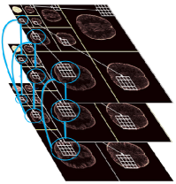
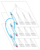
Figure 1: Forest structure on multi-contrast MR images. (a) Three multi-contrast MR images. (b) The wavelet coefficients of the images. Each coefficient tends to be consistent with its parent and children, and the coefficients across different trees at the same position. (c) One joint parent-child group across different trees that used in our algorithm.

Motivated by this limitation, we extend previous works to a more special but widely existed case. For multi-channel data, if it is jointly sparse, and more importantly, the common support of different channels yields a subtree structure, we call this kind of data forest-sparse data:

Definition 5: Forest-sparse data is defined as
$\mathcal{F}_{T,k}$={$X=[x_{1};x_{2};...;x_{T}]$: $x_{i}=\Phi^{-1}\theta_{i}$, $\theta_{i}|\Omega^{C}=0$, $|\Omega|=k$, where $\Omega$ forms a connected subtree, $i=1,2,...,T$ } .

Similarly, the forest-sparse data has forest sparsity property. This definition implies that if the coefficients at the same position across different channels are non-zeros, all their ancestor coefficients are all non-zeros. Learning with forest sparsity, we search the sparsest solution that follow the forest structure in the CS inverse problem. Any solution that violates the assumption will be penalized. Intuitively, the solution will be more accurate. We obtain our main result in the following theorem:

Theorem 3: For forest-sparse data, there exists a sub-Gaussian random matrix $A\in\mathbb{R}^{TM\times TN}$ that has the $\mathcal{F}_{T,k}$-RIP with probability $1-e^{-t}$ if the number of measurements satisfies that:

$$TM\geq\left\{\begin{matrix}\ \frac{2}{c_{1}\delta_{\mathcal{F}_{T,k}}}(k+\ln(N/(k+1))+Tk\ln(12/\delta_{\mathcal{F}_{T,k}})\\ +\ln 2+t)\qquad\textrm{if}\ k\leq\left\lfloor\log_{2}N\right\rfloor,\\ \ \frac{2}{c_{1}\delta_{\mathcal{F}_{T,k}}}(k\ln 4+\ln((c_{2}N)/k)+Tk\ln(12/\delta_{\mathcal{F}_{T,k}})\\ +\ln 2+t)\qquad\textrm{if}\ k>\left\lfloor\log_{2}N\right\rfloor.\end{matrix}\right.$$ (5)

where $c_{1}$ and $c_{2}$ are absolute constants.

For both cases, the bound is reduced to $M=\mathcal{O}(Tk+\log(N/k))$. The proofs of Lemma 1 as well as Lemma 2, 4 are included in the appendices. Using the $\mathcal{F}_{T,k}$-RIP, forest-sparse data can be robustly recovered from noisy compressive measurements.

Table I lists all the measurement bounds for the forest-sparse data with different models. Standard sparsity model only exploits the sparseness while no prior information about the locations of the non-zero elements is involved. It is the classical but worst model for forest-sparse data. These location priors are partially utilized in joint sparsity and tree sparsity models. One of them only studies the correlations across channels, while the other one only learns the intra structure. Our result is significantly better than those of joint sparsity and tree sparsity, and far better than that of standard sparsity, especially when $N/k$ is large. Only the proposed model fully exploits all these structures.

TABLE I: Measurement bounds for forest-sparse data

Sparse Models Measurement Bounds Standard Sparsity $\mathcal{O}(Tk+Tk\log(N/k))$ Joint Sparsity $\mathcal{O}(Tk+k\log(N/k))$ Tree Sparsity $\mathcal{O}(Tk+T\log(N/k))$ Forest Sparsity $\mathcal{O}(Tk+\log(N/k))$

So far, we have analyzed the result by forest sparsity over previous results. In all these results, the measurement matrix $A$ is assumed to be a dense sub-Gaussian matrix. However, in many practical problems, each data channel $x_{t}\in\mathbb{R}^{N}$ is measured by a distinct compressive matrix $A^{\prime}_{t}\in\mathbb{R}^{M\times N}$, $t=1,2,...,T$, which are called multiple measurement vectors (MMV) problems or multi-task learning ( e.g., [22, 49, 50]). Here and later, we assume that $\{A^{\prime}_{t}\}_{t=1}^{T}$ follow the same distribution but may be different. Therefore, the matrix $A$ is actually a block-diagonal matrix rather than a dense matrix. The linear system $b=Ax$ can be written as:

$$\begin{bmatrix}b_{1}\\ b_{2}\\ ...\\ b_{T}\end{bmatrix}=\begin{bmatrix}A^{\prime}_{1}&&&\\ &A^{\prime}_{2}&&\\ &&...&\\ &&&A^{\prime}_{T}\end{bmatrix}\begin{bmatrix}x_{1}\\ x_{2}\\ ...\\ x_{T}\end{bmatrix}$$ (6)

The non-diagonal blocks in $A$ are all zeros. Intuitively, such block-diagonal matrices have no better results than the dense matrices that discussed above, due to the less randomness. Unfortunately, the performance of the random block-diagonal matrices has not been analyzed on structured sparse data before, as all existing structured sparsity theories concentrate on the dense random matrix [17, 18, 19]. In this article, we extend the theoretical result to the block-diagonal matrix in the MMV problems.

Theorem 4: For forest-sparse data, there exists a block-diagonal matrix $A$ composed by sub-Gaussian random matrices $\{A^{\prime}_{t}\}_{t=1}^{T}$ as in (6), that has the $\mathcal{F}_{T,k}$-RIP with probability $1-e^{-t}$ if the number of measurements satisfies that:

$$TM\geq\left\{\begin{matrix}\ \frac{2T}{c_{1}W}(\ln 2+\ln(N/(k+1))+Tk\ln(12/\delta_{\mathcal{F}_{T,k}})\\ +k+t),\qquad\textrm{if}\ k\leq\left\lfloor\log_{2}N\right\rfloor,\\ \ \frac{2T}{c_{1}W}(\ln 2+\ln((c_{3}N)/k)+Tk\ln(12/\delta_{\mathcal{F}_{T,k}})\\ +k\ln 4+t),\qquad\textrm{if}\ k>\left\lfloor\log_{2}N\right\rfloor.\end{matrix}\right.$$ (7)

where $W=\min(c_{2}^{2}\delta_{\mathcal{F}_{T,k}}^{2}\Gamma_{2},c_{2}\delta_{\mathcal{F}_{T,k}}\Gamma_{\infty})$; $\Gamma_{2}=\frac{(\sum_{t=1}^{T}||x_{t}||^{2}_{2})^{2}}{\sum_{t=1}^{T}||x_{t}||^{4}_{2}}$ and $\Gamma_{\infty}=\frac{\sum_{t=1}^{T}||x_{t}||^{2}_{2}}{\max_{t=1}^{T}||x_{t}||^{2}_{2}}$; $c_{1}$, $c_{2}$ and $c_{3}$ are absolute constants.

For both cases, the bound can be written as $TM=\mathcal{O}(\frac{T^{2}k+T\log(N/k)}{\min(\Gamma_{2},\Gamma_{\infty})})$. In contrast to previous results on dense matrices with i.i.d sub-Gaussian entries, this bound also depends on the energy of the data. It is not hard to find that $1\leq\Gamma_{2}\leq T$ and $1\leq\Gamma_{\infty}\leq T$. In the best case, when $||x_{1}||_{2}=||x_{2}||_{2}=...=||x_{T}||_{2}$ and $\Gamma_{2}=\Gamma_{\infty}=T$, the measurement bound is $TM=\mathcal{O}({Tk+\log(N/k)}$. It shows a similar performance as the dense sub-Gaussian matrix in Theorem 3. In the worst case, the energy of the data concentrate on one single channel/task, i.e., all $||x_{t}||_{2}=0$ except a single index $||x_{t^{\prime}}||_{2}\neq 0$. The measurement bound then is $TM=\mathcal{O}({T^{2}k+T\log(N/k)}$, which is even worse than that in Theorem 2 for independent tree sparse channels. Even for the same block-diagonal matrix, the analysis makes clear that its performance may varies significantly depending on the data being measured. In the worst case, their measurement bound can increase $T$ times. However, the increased factor $T/\min(c_{2}^{2}\delta^{2}\Gamma_{2},c_{2}\delta\Gamma_{\infty})$ for block-diagonal matrices also applies to standard sparse data, joint sparse data and tree sparse data. For the same measurement matrix and the same data, the advantage of forest sparsity still exists. Due to this reason, we do not evaluate the term $\min(c_{2}^{2}\delta^{2}\Gamma_{2},c_{2}\delta\Gamma_{\infty})$ in the experiments, while focus our interest on comparing different sparsity models on the same data.

IV Algorithm

In this article, the forest structure is approximated as overlapping group sparsity [44] with mixed $\ell_{2,1}$ norm. Although it may not be the best approximation, it is enough to demonstrate the benefit of forest sparsity. To evaluate the forest sparsity model, we need to compare different models via a similar framework. From the definition of forest-sparse data, we could find that a coefficient is large/small, its parent and ”neighbors” also tend to be large/small. All parent-child pairs in the same position across different channels are assigned into one group, and the problem becomes overlapping group sparsity regularization. Similar scheme has been used in approximating tree sparsity [39, 40], where each node and its parent are assigned into one group. We write the approximated problem as:

$$\min_{x}\frac{1}{2}||Ax-b||_{2}^{2}+\lambda\sum_{g\in\mathcal{G}}||(\Phi x)_{g}||_{2}$$ (8)

where $g$ denotes one of the coefficient groups discussed above (an example is demonstrated in Fig.1(c)), $(\cdot)_{g}$ denotes the coefficients in group $g$ and $\mathcal{G}$ is the set of all groups.

The mixed $\ell_{2,1}$ norm encourages all the components in the same group $g$ to be zeros or non-zeros simultaneously. With our group configuration, it encourages forest sparsity. We present an efficient implementation based on fast iterative shrinkage-thresholding algorithm (FISTA) [12] framework for this problem. This is because FISTA can be easily applied for standard sparsity and joint sparsity, which could make the validation of the benefit of the proposed model more convenient. In addition, the formulation (8) can be easily extended to the combination of total variation (TV) via the Fast Composite Splitting Algorithms (FCSA) scheme [51]. Note that other algorithms may be used to solve the forest sparsity problems, e.g. [32, 44, 52], but determining the optimal algorithm for forest sparsity is not the scope of this article.

FISTA [12] is a accelerated version of proximal method which minimizes the object function with the following form:

$$\min\{F(x)=f(x)+g(x)\}$$ (9)

where $f(x)$ is a convex smooth function with Lipschitz constant $L_{f}$ and $g(x)$ is a convex but usually nonsmooth function. It comes to the original FISTA when $f(x)=\frac{1}{2}||Ax-b||_{2}^{2}$ and $g(x)=\lambda\|\Phi x\|_{1}$, which is summarized in Algorithm 1, where, $A^{T}$ denotes the transpose of $A$.

Algorithm 1 FISTA [12]

  Input: $\rho={1}/{L_{f}}$, $\lambda$, $n=1$, $t^{1}=1$ $r^{1}=x^{0}$

  while not meet the stopping criterion do

     $y=r^{n}-\rho A^{T}(Ar^{n}-b)$

     $x=\arg\min_{x}\{\frac{1}{2\rho}\|x-y\|^{2}+\lambda\|\Phi x\|_{1}\}$

     $t^{n+1}={1+\sqrt{1+4(t^{n})^{2}}}/{2}$

     $r^{n+1}=x^{n}+\frac{t^{n}-1}{t^{n+1}}(x^{n}-x^{n-1})$

     $n=n+1$

  end while

For the second step, there is closed form solution by soft-thresholding. For joint sparsity problem where $g(x)=\lambda\|\Phi x\|_{2,1}$, the second step also has closed form solution. We call the version as FISTA_Joint for joint sparsity. However, for the problem (8) with overlapped groups, we can not directly apply FISTA to solve it.

In order to transfer the problem (8) to non-overlapping version, we introduce a binary matrix $G\in\mathbb{R}^{D\times TN}$ ($D>TN$) to duplicate the overlapped coefficients. Each row of $G$ only contains one 1 and all else are 0s. The 1 appears in the $i$-th column corresponds to the $i$-th coefficient of $\Phi x$. Intuitively, if the coefficient is included in $j$ groups, $G$ will contains $j$ such rows. An auxiliary variable $z$ is used to constrain $G\Phi x$. This scheme is widely utilized in the alternating direction method (ADM) [32]. The alternating formulation becomes:

$$\vspace{-0.0cm}\min_{x,z}\{\frac{1}{2}\|Ax-b\|_{2}^{2}+\lambda\sum_{g\in\mathcal{G}}||z_{g}||_{2}+\frac{\gamma}{2}||z-G\Phi x||_{2}^{2}\}\vspace{-0.0cm}$$ (10)

where $\gamma$ is another positive parameter. We iteratively solve this alternative formulation by minimizing $x$ and $z$ subproblems respectively. For the $z$ subproblem:

$$\hat{z_{g}}=\arg\min_{z_{g}}\{\lambda||z_{g}||_{2}+\frac{\gamma}{2}||z_{g}-(G\Phi x)_{g}||_{2}^{2}\},g\in\mathcal{G}$$ (11)

which has the closed form solution:

$$\hat{z_{g}}=\max(||(G\Phi x)_{g}||_{2}-\frac{\lambda}{\gamma},0)\frac{(G\Phi x)_{g}}{||(G\Phi x)_{g}||_{2}},g\in\mathcal{G}$$ (12)

We denote it as a shrinkgroup operation. For the $x$-subproblem:

$$\hat{x}=\arg\min_{x}\{\frac{1}{2}\|Ax-b\|_{2}^{2}+\frac{\gamma}{2}||z-G\Phi x||_{2}^{2}\}$$ (13)

The optimal solution is $x=(A^{T}A+\lambda\Phi^{T}G^{T}G\Phi)^{-1}(A^{T}b+\lambda\Phi^{T}G^{T}z)$, which contains a large scale inverse problem. Actually, this problem can be efficient solved by various methods. In order to compare with FISTA and FISTA_Joint, we apply FISTA to solve (13). This could demonstrate the benefit of forest sparsity more clearly. Let $f(x)=\frac{1}{2}\|Ax-b\|_{2}^{2}+\frac{\lambda}{2}||z-G\Phi x||_{2}^{2}$ and $g(x)=0$. Supposing its Lipschitz constant to be $L_{f}$, the whole algorithm is summarized in Algorithm 2.

Algorithm 2 FISTA_Forest

  Input: $\rho=1/L_{f}$, $r^{1}=x^{0}$, $t^{1}=1,\lambda,\gamma,n=1$

  while not meet the stopping criterion do

     $z=shrinkgroup(G\Phi x^{n-1},\lambda/\gamma)$

     $x^{n}=r^{n}-\rho[A^{T}(Ar^{n}-b)+\gamma\Phi^{T}G^{T}(G\Phi r^{n}-z)]$

     $t^{n+1}=[1+\sqrt{1+4(t^{n})^{2}}]/2$

     $r^{n+1}=x^{n}+\frac{t^{n}-1}{t^{n+1}}(x^{n}-x^{n-1})$

     $n=n+1$

  end while

For the first step, we solve (11) while $\frac{1}{2}\|Ax-b\|_{2}^{2}$ keeps the same. The object function value in (10) decreases. For the second step, (13) is solved by FISTA iteratively while $\lambda\sum_{g\in\mathcal{G}}||z_{g}||_{2}$ keeps the same. Therefore, the object function value in (10) decreases in each iteration and the algorithm is convergent. Algorithm 2 is also used to implement tree sparsity by recovering the data channel-by-channel separately. We call it FISTA_Tree.

In some practical applications, the data tends to be forest-sparse but not strictly. We can soften and complement the forest assumption with other penalties, such as joint $\ell_{2,1}$ norm or TV. For example, after combining TV, problem (10) becomes:

$$\vspace{-0.0cm}\min_{x,z}\{\frac{1}{2}\|Ax-b\|_{2}^{2}+\lambda\sum_{g\in\mathcal{G}}||z_{g}||_{2}+\frac{\gamma}{2}||z-G\Phi x||_{2}^{2}$$

$$+\mu||x||_{TV}\}\vspace{-0.0cm}$$ (14)

where $||x||_{TV}=\sum_{i=1}^{TN}\sqrt{(\nabla_{1}x_{i})^{2}+(\nabla_{2}x_{i})^{2}}$; $\nabla_{1}$ and $\nabla_{2}$ denote the forward finite difference operators on the first and second coordinates respectively; $\mu$ is a positive parameter. Compared with Algorithm 2, we only need to set $g(x)=\mu||x||_{TV}$ and the corresponding subproblem has already been solved [12, 51, 53]. This TV combined algorithm is called FCSA_Forest, which will be used in the experiments. To avoid repetition, it is not listed.

V Applications and Experiments

We conduct experiments on the RGB color image, multi-contrast MR images, MR image of multi-channel coils and the multispectral image to validate the benefit of forest sparsity. All experiments are conducted on a desktop with 3.4GHz Intel core i7 3770 CPU. Matlab version is 7.8(2009a). If the sampling matrix $A$ is $M$ by $N$, the sampling ratio is defined as $M/N$. All measurements are mixed with Gaussian white noise of 0.01 standard deviation. Signal-to-Noise Ratio (SNR) is used as the metric for evaluations:

$$SNR=10\log_{10}(V_{s}/V_{n})$$ (15)

where $V_{n}$ is the Mean Square Error between the original data $x_{0}$ and the reconstructed $x$; $V_{s}=var(x_{0})$ denotes the power level of the original data where $var(x_{0})$ denotes the variance of the values in $x_{0}$.

V-A Multi-contrast MRI

Multi-contrast MRI is a popular technique to aid clinical diagnosis. For example T1 weighted MR images could distinguish fat from water, with water appearing darker and fat brighter. In T2 weighted images fat is darker and water is lighter, which is better suited to imaging edema. Although with different intensities, T1/T2 or proton-density weighted MR images are scanned at the same anatomical position. Therefore they are not independent but highly correlated. Multi-contrast MR images are typically forest-sparse under the wavelet basis. Suppose $\{x_{t}\}_{t=1}^{T}\in\mathbb{R}^{N}$ are the multi-contrast images for the same anatomical cross section and $\{b_{t}\}_{t=1}^{T}$ are the corresponding undersampled data in Fourier domain, the forest-sparse reconstruction can be formulated as:

$$\hat{x}=\arg\min_{x}\|\Phi x\|_{\mathcal{F},T}+\lambda\sum_{s=1}^{T}\|R_{t}x_{t}-b_{t}\|^{2}$$ (16)

where $x$ is the vertorized data of $[x_{1},...,x_{T}]$ and $R_{t}$ is the measurement matrix for the image $x_{t}$. This is an extension of conventional CS-MRI [54]. Fig. 1 shows an example of the forest structure in multi-contrast MR images.

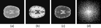
Figure 2: (a)-(c) the original multi-constrast images and (d) the sampling mask.

The data is extracted from the SRI24 Multi-Channel Brain Atlas Dataset [55]. In the Fourier domain, we randomly obtain more samples in low frequencies and less samples in higher frequencies. This sampling scheme has been widely used for CS-MRI [54, 56, 51]. Fig. 2 shows the original multi-contrast MR images and the sampling mask.

We compare four algorithms on this dataset: FISTA, FISTA_Joint, FISTA_Tree and FISTA_Forest. The parameter $\lambda$ is set 0.035, and $\gamma$ is set to $0.5\lambda$. We run each algorithm 400 iterations. Fig. 3 (a) demonstrates the performance comparisons among different algorithms. From the figure, we could observe that modeling with forest sparsity achieves the highest SNR after convergence. Although the algorithm for forest sparsity takes more time due to the overlapping structure, it always outperforms all others in terms of accuracy.

In addition, as total variation is very popular in CS-MRI [54, 51, 25], we compare our FCSA_Forest algorithm with FCSA [51] (TV is combined in FISTA), FCSA_Joint [25] (TV is combined in FISTA_Joint) and FCSA_Tree. The parameter $\mu$ for TV is set $0.001$, the same as that in previous works [56, 51]. Fig. 3 (b) demonstrates the performance comparison including TV regularization. Compared with Fig. 3 (a), all algorithms improve at different degrees. However, the ranking does not change, which validates the superiority of forest sparsity. As FCSA has been proved to be better than other algorithms for general compressive sensing MRI (CS-MRI) [54, 56, 57] and FCSA_Joint [25] better than [24, 58] in multi-contrast MRI, the proposed method further improves CS-MRI and make it more feasible than before.

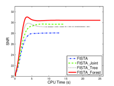
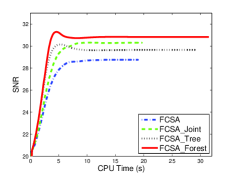
Figure 3: Performance comparisons among different algorithms. (a) Multi-constrast MR images reconstruction with $20\%$ sampling. Their final SNRs are 28.05, 29.69, 29.22 and 30.42 respectively. The time costs are 13.11s, 14.43s, 22.08s and 25.11s respectively. (b) Multi-constrast MR images reconstruction with $20\%$ sampling by both wavelet sparsity and TV regularization. Their final SNRs are 28.75, 30.30, 29.65 and 30.83 respectively. The time costs are 19.00s, 19.68s, 29.11s and 31.41s respectively.

In order to validate the benefit of forest sparsity in terms of measurement number, we conduct an experiment to reconstruct multi-contrast MR images from different sampling ratios. Fig. 4 demonstrates the final results of four algorithms with sampling ratio from $16\%$ to $26\%$. With more sampling, all algorithms have better performance. However, The forest sparsity algorithm always achieves the best reconstruction. For the same reconstruction accuracy, the FISTA_Forest algorithm only requires about $16\%$ measurements to achieve SNR 28, which is approximately $2\%$, $3\%$, $5\%$ less than that of FISTA_Joint, FISTA_Tree and FISTA respectively. More results of forest sparsity on multi-contrast MRI can be found in [59].

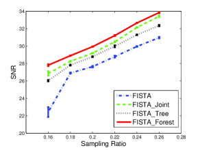
Figure 4: Reconstruction performance with different sampling ratios.

V-B parallel MRI

To improve the scanning speed of MRI, an efficient and feasible way is to acquire the data in parallel with multi-channel coils. The scanning time depends on the number of measurements in Fourier domain, and it will be significantly reduced when each coil only acquires a small fraction of the whole measurements. The bottleneck is how to reconstruct the original MR image efficiently and precisely. This issue is called pMRI in literature. Sparsity techniques have been used to improve the classical method SENSE [60]. However, when the coil sensitivity can not be estimated precisely, the final image would contain visual artifacts. Unlike previous CS-SENSE [61] which reconstructs the images of multi-coils individually, calibrationless parallel MRI [62, 63] recovers the aliased images of all coils jointly by assuming the data is jointly sparse.

Let $T$ equal to the number of coils and $b_{t}$ be the measurement vector from coil $t$. It is therefore the same CS problem as (16). The final result of CaLM-MRI is obtained by a sum of square (SoS) approach without coil sensitivity and SENSE encoding. It shows comparable results with those methods which need precise coil configuration. As shown in Fig. 5, the appearances of different images obtained from multi-coils are very similar. This method can be improved with forest sparsity, since the images follow the forest sparsity assumption.

Figure 5: The aliased MR images of multi-coils. Due to the different locations of the coils, they have different sensitivities to the same image.

There are two steps for compressive sensing pMRI reconstruction in CaLM-MRI [62]: 1) the aliased images are recovered from the undersampled Fourier signals of different coil channels by CS methods; 2) The final image for clinical diagnosis is synthesized by the recovered aliased images using the sum-of-square (SoS) approach. As discussed above, these aliased images should be forest-sparse under the wavelet basis. We compare our algorithm with FISTA_Joint and SPGL1 [31] which solves the joint $\ell_{2,1}$ norm problem in CaLM-MRI. For the second step, all methods use the SoS approach from the aliased images that they recovered. All algorithms run enough time until it has converged.

TABLE II: Comparisons of SNRs (dB) on different sampling ratios with $4$ coils

sampling ratios 25% 20% 17% 15% SNR of SPGL1 26.72 24.59 23.08 22.31 Aliased Images FISTA_Joint 26.95 24.73 23.06 22.21 FISTA_Forest 27.47 25.22 23.37 22.59 SNR of SPGL1 20.64 20.35 19.12 18.64 Final Image FISTA_Joint 20.79 20.41 19.75 18.49 FISTA_Forest 22.62 22.29 21.03 20.47

TABLE III: Comparisons of SNRs (dB) on different number of coils with $20\%$ sampling

number of coils 2 4 6 8 SNR of SPGL1 23.33 24.61 24.74 25.16 Aliased Images FISTA_Joint 23.41 24.71 24.89 25.23 FISTA_Forest 24.25 25.12 25.29 25.52 SNR of SPGL1 21.76 18.95 21.05 21.32 Final Image FISTA_Joint 21.90 18.94 21.15 21.87 FISTA_Forest 22.44 22.22 22.52 22.52

Table II and Table III show all the comprehensive comparisons among these algorithms. For the same algorithm, more measurements or more number of coils tend to increase the SNRs of aliased images, although it does not result in linear improvement for the final image reconstruction. Another observation is that FISTA_Joint and SPGL1 have similar performance in terms of SNR on this data. This is because both of them solve the same joint sparsity problem, even with different schemes. Upgrading the model to forest sparsity, significant improvement can be gained. Finally, it is unknown how to combine TV in SPGL1. However, both FISTA_Joint and FISTA_Forest can easily combine TV, which can further enhance the results [25].

V-C Color Image Reconstruction

Color images captured by optical camera can be represented as combinations of red, green, blue three colors. Different colors synthesized by these three colors seems realistic to human eyes. By observing the color channels are highly correlated, joint sparsity prior is utilized in recent recovery [23]. Modeling with $\ell_{2,1}$ norm regularization can gain additional SNR to standard $\ell_{1}$ norm regularization. Further more, each color channel tends to be wavelet tree-sparse. If we model the problem with forest sparsity, this result would be reasonably better.

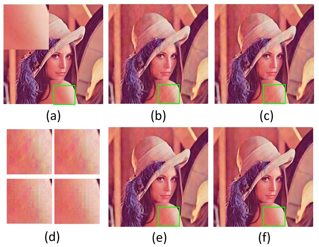
Figure 6: Visual comparisons on the lena image reconstruction after 50 iterations with about $20\%$ sampling. (a) the original image and the patch detail; (b) recovered by FISTA; (c) recovered by FISTA_Joint; (d) the patch details for each recovered image; (e) recovered by FISTA_Tree; (f) recovered by FISTA_Forest. Their SNRs are 16.65, 17.41, 17.66 and 18.92, respectively.

For color images, we compare our algorithm with FISTA, FISTA_Joint and FISTA_Tree. Fig. 6 shows the visual results recovered by different sparse penalties. Only after 50 iterations, the image recovered by our algorithm is very close to the original one with the fewest artifacts (shown in the zoomed region of interest).

V-D Multispectral Image Reconstruction

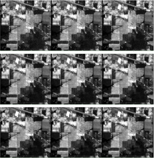
Figure 7: The original multispectral image: band 6 to band 14.

Different from common color images, a multispectral or hyperspectral image is consisted of much more bands, which provides both spatial and spectral representations of scenes. It is widely utilized on remote sensing with applications to agriculture, environment detection etc.. However, the collection of large amount of data costs both huge imaging time and storage space. By compressive sensing data acquisition, the cost of imaging for remote sensing data could be significantly reduced [64]. Like RGB images, the bands of multispectral image should represent the same scene. Each band has tree sparsity property. Therefore, they follow the forest sparsity assumption. Fig. 7 shows bands 6 to 14 of a multispectral image of 1992 AVIRIS Indian Pine Test Site 3 .

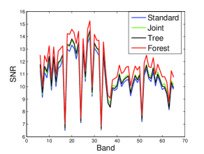
Figure 8: Multispectral image reconstruction results by different sparse models with about $20\%$ sampling.

For multispectral image, we test a dataset of 1992 AVIRIS image Indian Pine Test Site 3 (examples shown in Fig. 7). It is a $2\times 2$ mile portion of Northwest Tippecanoe County of Indiana. There are total $220$ bands. Each band is recovered separately for standard sparsity and tree sparsity, while every 3 bands are reconstructed simultaneously by joint-sparse model and forest-sparse model. Each image is cropped to $128\times 128$ for convenience. The number of wavelet decomposition levels is set to 3. The SNRs of all recovered images for band 6 to 66 are shown in Fig. 8. One could observe that modeling with forest sparsity always achieves the highest SNRs, which validates the benefit of forest sparsity.

VI Conclusion

In this paper, we have proposed a novel model forest sparsity for sparse learning and compressive sensing. This model enriches the family of structured sparsity and can be widely applied on numerous fields of sparse regularization problems. The benefit of the proposed model has been theoretically proved and empirically validated in practical applications. Under compressive sensing assumptions, significant reduction of measurements is achieved with forest sparsity compared with standard sparsity, joint sparsity or independent tree sparsity. A fast algorithm is developed to efficiently solve the forest sparsity problem. While applying it on practical applications such as multi-contrast MRI, pMRI, multispectral image and color image reconstruction, extensive experiments demonstrate the superiority of forest sparsity over standard sparsity, joint sparsity and tree sparsity in terms of both accuracy and computational complexity.

Appendix A Proof of Theorem 2

The proof is conducted on the binary tree case for convenience. The bound for quadtree can be easily extended.

First, we need to figure out the number of subtrees (size $k$) of a binary tree (size $N$). Note that the root of the subtrees should be the binary tree’s root.

Case 1: when $k\leq\left\lfloor\log_{2}N\right\rfloor$, the number of subtrees of size $k$ is just the Catalan number:

$$L_{\mathcal{T}}=\frac{1}{k+1}\binom{2k}{k}\leq\frac{(2e)^{k}}{k+1}\leq\frac{e^{k}N}{k+1}.$$ (17)

Case 2: when $k>\left\lfloor\log_{2}N\right\rfloor$, the number of subtrees of size $k$ should follow [18]:

$$L_{\mathcal{T}} \leq\frac{4^{k}}{k}(\frac{6}{\sqrt{\pi k}}\ln\frac{\log_{2}N}{\left\lfloor\log_{2}k\right\rfloor)}+\frac{128}{e^{2}\left\lfloor\log_{2}k\right\rfloor})$$

$$\leq\frac{4^{k}}{k}(\frac{c_{1}\log_{2}N}{\left\lfloor\log_{2}k\right\rfloor)}+\frac{c2}{\left\lfloor\log_{2}k\right\rfloor})$$

$$\leq\frac{4^{k}}{k}\frac{c_{1}\log_{2}(c_{3}N)}{\log_{2}k}$$

$$\leq\frac{4^{k}(c_{4}N)}{k}.$$ (18)

where $c_{1}$, $c_{2}$, $c_{3}$, $c_{4}$ are some constants. Therefore we have:

$$L_{\mathcal{T}}\leq\left\{\begin{matrix}\frac{e^{k}N}{k+1}&\textrm{if}\ k\leq\left\lfloor\log_{2}N\right\rfloor,\\ \frac{4^{k}(c_{4}N)}{k}&\textrm{if}\ k>\left\lfloor\log_{2}N\right\rfloor.\end{matrix}\right.$$ (19)

According to Theorem 1:

$$M\geq\frac{2}{c\delta}(\ln(2L)+k\ln\frac{12}{\delta}+t).$$ (20)

With (20), the number of measurements should satisfy:

$$M\geq\left\{\begin{matrix}\ \frac{2}{c\delta_{\mathcal{T}_{k}}}(k+\ln(N/(k+1))+k\ln(12/\delta_{\mathcal{T}_{k}})\\ +\ln 2+t)\qquad\textrm{if}\ k\leq\left\lfloor\log_{2}N\right\rfloor,\\ \ \frac{2}{c\delta_{\mathcal{T}_{k}}}(k\ln 4+\ln(c_{4}N/k)+k\ln(12/\delta_{\mathcal{T}_{k}})\\ +\ln 2+t)\qquad\textrm{if}\ k>\left\lfloor\log_{2}N\right\rfloor.\end{matrix}\right.$$ (21)

For both cases, we have $M=\mathcal{O}(k+\log(N/k))$ as the minimum number of measurements. Similar bound also has been proved in previous papers [18] [17].

Appendix B Proof of Theorem 3

If the data is forest-sparse, the support set of different trees are dependent. It means if the support set for one tree is fixed, then all support sets for other trees are fixed. Accordingly, the number of combinations is still $L_{\mathcal{T}}$. Note that the sparsity number is $Tk$ as there are $T$ trees. Therefore,

$$TM\geq\left\{\begin{matrix}\ \frac{2}{c\delta_{\mathcal{F}_{T,k}}}(k+\ln(N/(k+1))+Tk\ln(12/\delta_{\mathcal{F}_{T,k}})\\ +\ln 2+t)\qquad\textrm{if}\ k\leq\left\lfloor\log_{2}N\right\rfloor,\\ \ \frac{2}{c\delta_{\mathcal{F}_{T,k}}}(k\ln 4+\ln((c_{4}N)/k)+Tk\ln(12/\delta_{\mathcal{F}_{T,k}})\\ +\ln 2+t)\qquad\textrm{if}\ k>\left\lfloor\log_{2}N\right\rfloor.\end{matrix}\right.$$ (22)

For both cases, the bound is reduced to $TM=\mathcal{O}(Tk+\log(N/k))$.

Appendix C Proof of Theorem 4

We first derive the sufficient condition that guarantees the RIP for block-diagonal matrices.

Theorem 5. Let a matrix $A\in\mathbb{R}^{TM\times TN}$ be composed by sub-Gaussian random matrices $\{A^{\prime}_{t}\in\mathbb{R}^{M\times N}\}_{t=1}^{T}$ as in (6). For any fixed subset $S\subset\{1,2,...,TN\}$ with $|S|=TK$ and $0<\delta<1$, we have with probability exceeding $1-2(12/\delta)^{TK}e^{-c_{1}\frac{M}{2}\min(c_{2}^{2}\delta^{2}\Gamma_{2},c_{2}\delta\Gamma_{\infty})}$:

$$(1-\delta)||X||_{2}\leq||A_{S}X||_{2}\leq(1+\delta)||X||_{2},$$ (23)

for all $X=[x_{1};x_{2};...;x_{T}]\in\mathbb{R}^{Tk\times 1}$. $c_{1}$ and $c_{2}$ are absolute constants, $\Gamma_{2}=\frac{(\sum_{t=1}^{T}||x_{t}||^{2}_{2})^{2}}{\sum_{t=1}^{T}||x_{t}||^{4}_{2}}$ and $\Gamma_{\infty}=\frac{\sum_{t=1}^{T}||x_{t}||^{2}_{2}}{\max_{t=1}^{T}||x_{t}||^{2}_{2}}$.

Proof. Let’s denote $\bar{X}=X/||X||_{2}$ and we have $||\bar{X}||_{2}=1$. We choose a finite set of points $Q=\{q_{i}\}$, such that $q_{i}\in\mathbb{R}^{Tk\times 1}$ and $||q_{i}||_{2}=1$ for all $i$. We have $\min_{i}||\bar{X}-q_{i}||^{2}\leq\epsilon_{1}$ and covering number satisfies $|Q|\leq(1+2/\epsilon_{1})^{TK}$ for any $\epsilon_{1}>0$ (see Chap 13 of [65]).

As the block-diagonal matrix $A$ is composed by sub-Gaussian random matrices, we have for each $i$ and any $\epsilon_{2}>0$:

$$\mathrm{P}(|||Aq_{i}||_{2}^{2}-||q_{i}||_{2}^{2}|\geq \epsilon_{2}||q_{i}||_{2}^{2})$$

$$\leq 2e^{-c_{1}\frac{M}{2}\min(c_{2}^{2}\epsilon_{2}^{2}\Gamma_{2},c_{2}\epsilon_{2}\Gamma_{\infty})},$$ (24)

with $\Gamma_{2}$ and $\Gamma_{\infty}$ defined above. This probability is indicated in Theorem III.1 of [66].

Taking union bound, we obtain with probability exceeding $1-2(1+2/\epsilon_{1})^{TK}e^{-c_{1}\frac{M}{2}\min(c_{2}^{2}\epsilon_{2}^{2}\Gamma_{2},c_{2}\epsilon_{2}\Gamma_{\infty})}$:

$$(1-\epsilon_{2})\leq||A_{S}q_{i}||_{2}^{2}\leq(1+\epsilon_{2}),\ \mathrm{for}\ \mathrm{all}\ q_{i}\in Q,$$ (25)

which gives

$$(1-\epsilon_{2})\leq||A_{S}q_{i}||_{2}\leq(1+\epsilon_{2}),\ \mathrm{for}\ \mathrm{all}\ q_{i}\in Q.$$ (26)

Now we define $\rho$ as the smallest nonnegative number such that

$${||A_{S}\bar{X}||_{2}}\leq(1+\rho),$$ (27)

for all $\bar{X}\in\mathbb{R}^{Tk\times 1}$ and $||\bar{X}||_{2}=1$. We have

$${||A_{S}\bar{X}||_{2}} \leq{||A_{S}q_{i}||_{2}+||A_{s}(\bar{X}-q_{i})||_{2}}$$

$$\leq{||A_{S}q_{i}||_{2}}+{||A_{s}(\bar{X}-q_{i})||_{2}}$$

$$\leq(1+\epsilon_{2})+(1+\rho)\epsilon_{1}.$$ (28)

As $\rho$ as the smallest nonnegative number for (27), we have:

$$1+\rho\leq(1+\epsilon_{2})+(1+\rho)\epsilon_{1},$$ (29)

and

$$\rho\leq(\epsilon_{1}+\epsilon_{2})/(1-\epsilon_{1}).$$ (30)

Note the above result holds for any $\epsilon_{1}$ and $\epsilon_{2}$. We choose $\epsilon_{1}=\delta/4$ and $\epsilon_{2}=\delta/2$. Since $0<\delta<1$, it is easy to see that $\rho\leq\delta$, which proves

$${||A_{S}\bar{X}||_{2}}\leq(1+\delta).$$ (31)

Similar, ${(1-\delta)\leq||A_{S}\bar{X}||_{2}}$ can be proved using the same way. Finally, we obtain with probability exceeding $1-2(12/\delta)^{TK}e^{-c_{1}\frac{M}{2}\min(c_{2}^{2}\delta^{2}\Gamma_{2},c_{2}\delta\Gamma_{\infty})}$:

$$(1-\delta)\leq\frac{||A_{S}X||_{2}}{||X||_{2}}\leq(1+\delta),$$ (32)

which completes the proof as $1+2/\epsilon_{1}=(\delta+8)/\delta\leq 12/\delta$.

Based on this theorem, we know that any $Tk$-sparse $X\in\mathbb{R}^{TN\times 1}$ satisfies

$$(1-\delta)||X||_{2}\leq||AX||_{2}\leq(1+\delta)||X||_{2},$$ (33)

with probability exceeding $1-2(12/\delta)^{TK}e^{-c_{1}\frac{M}{2}\min(c_{2}^{2}\delta^{2}\Gamma_{2},c_{2}\delta\Gamma_{\infty})}$.

Suppose there are $L$ combinations of such set $S$, from appendix A and B we know that

$$L\leq\left\{\begin{matrix}\frac{e^{k}N}{k+1}&\textrm{if}\ k\leq\left\lfloor\log_{2}N\right\rfloor,\\ \frac{4^{k}(c_{4}N)}{k}&\textrm{if}\ k>\left\lfloor\log_{2}N\right\rfloor.\end{matrix}\right.$$ (34)

for forest sparse data.

By taking the union bound, we known that (23) fails with probability less than

$$2L(12/\delta_{\mathcal{F}_{T,k}})^{TK}e^{-c_{1}\frac{M}{2}\min(c_{2}^{2}\delta_{\mathcal{F}_{T,k}}^{2}\Gamma_{2},c_{2}\delta_{\mathcal{F}_{T,k}}\Gamma_{\infty})}\leq e^{-t},$$ (35)

which gives

$$TM\geq\left\{\begin{matrix}\ \frac{2T(\ln 2+k+\ln(N/(k+1))+Tk\ln(12/\delta_{\mathcal{F}_{T,k}})+t)}{c_{1}\min(c_{2}^{2}\delta_{\mathcal{F}_{T,k}}^{2}\Gamma_{2},c_{2}\delta_{\mathcal{F}_{T,k}}\Gamma_{\infty})},\vspace{0.15cm}\\ \qquad\textrm{if}\ k\leq\left\lfloor\log_{2}N\right\rfloor,\vspace{0.15cm}\\ \ \frac{2T(\ln 2+k\ln 4+\ln((c_{3}N)/k)+Tk\ln(12/\delta_{\mathcal{F}_{T,k}})+t)}{c_{1}\min(c_{2}^{2}\delta_{\mathcal{F}_{T,k}}^{2}\Gamma_{2},c_{2}\delta_{\mathcal{F}_{T,k}}\Gamma_{\infty})},\vspace{0.15cm}\\ \qquad\textrm{if}\ k>\left\lfloor\log_{2}N\right\rfloor.\end{matrix}\right.$$ (36)

From this one theorem 4 can be easily derived. For both cases, the bound can be written as $TM=\mathcal{O}(\frac{T^{2}k+T\log(N/k)}{\min(\Gamma_{2},\Gamma_{\infty})})$.

References

- [1] E. Candès, J. Romberg, and T. Tao, “Robust uncertainty principles: Exact signal reconstruction from highly incomplete frequency information,” IEEE Trans. Inf. Theory, vol. 52, no. 2, pp. 489–509, 2006.
- [2] D. Donoho, “Compressed sensing,” IEEE Trans. Inf. Theory, vol. 52, no. 4, pp. 1289–1306, 2006.
- [3] E. Candès, “Compressive sampling,” in Proc. Int. Congr. Math., 2006, pp. 1433–1452.
- [4] E. Candes and J. Romberg, “Sparsity and incoherence in compressive sampling,” Inverse problems, vol. 23, no. 3, p. 969, 2007.
- [5] E. Candes, J. Romberg, and T. Tao, “Stable signal recovery from incomplete and inaccurate measurements,” Comm. Pure Appl. Math., vol. 59, no. 8, pp. 1207–1223, 2006.
- [6] B. Natarajan, “Sparse approximate solutions to linear systems,” SIAM J. Sci. Comput., vol. 24, no. 2, pp. 227–234, 1995.
- [7] R. Tibshirani, “Regression shrinkage and selection via the lasso,” J. R. Stat. Soc. Series B Stat. Methodol., pp. 267–288, 1996.
- [8] S. Chen, D. Donoho, and M. Saunders, “Atomic decomposition by basis pursuit,” SIAM J. Sci. Comput., vol. 20, no. 1, pp. 33–61, 1998.
- [9] D. Donoho and M. Elad, “Optimally sparse representation in general (nonorthogonal) dictionaries via minimization,” Optimally, vol. 100, no. 5, pp. 2197–2202, 2002.
- [10] J. Tropp, “Greed is good: Algorithmic results for sparse approximation,” IEEE Trans. Inf. Theory, vol. 50, no. 10, pp. 2231–2242, 2004.
- [11] D. Needell and J. Tropp, “CoSaMP: Iterative signal recovery from incomplete and inaccurate samples,” Appl. Computat. Harmon. Anal., vol. 26, no. 3, pp. 301–321, 2009.
- [12] A. Beck and M. Teboulle, “A fast iterative shrinkage-thresholding algorithm for linear inverse problems,” SIAM J. Imaging Sci., vol. 2, no. 1, pp. 183–202, 2009.
- [13] M. Figueiredo, R. Nowak, and S. Wright, “Gradient projection for sparse reconstruction: Application to compressed sensing and other inverse problems,” IEEE J. Sel. Topics Signal Process., vol. 1, no. 4, pp. 586–597, 2007.
- [14] K. Koh, S. Kim, and S. Boyd, “An interior-point method for large-scale l1-regularized logistic regression,” J. Mach. Learn. Res., vol. 8, no. 8, pp. 1519–1555, 2007.
- [15] S. Ji, Y. Xue, and L. Carin, “Bayesian compressive sensing,” IEEE Trans. Signal Process., vol. 56, no. 6, pp. 2346–2356, 2008.
- [16] D. Donoho, A. Maleki, and A. Montanari, “Message-passing algorithms for compressed sensing,” in Proc. National Academy of Sciences, vol. 106, no. 45, 2009, pp. 18 914–18 919.
- [17] J. Huang, T. Zhang, and D. Metaxas, “Learning with structured sparsity,” J. Mach. Learn. Res., vol. 12, pp. 3371–3412, 2011.
- [18] R. Baraniuk, V. Cevher, M. Duarte, and C. Hegde, “Model-based compressive sensing,” IEEE Trans. Inf. Theory, vol. 56, no. 4, pp. 1982–2001, 2010.
- [19] J. Huang, “Structured sparsity: theorems, algorithms and applications,” Ph.D. dissertation, Rutgers University, 2011.
- [20] J. Meng, W. Yin, H. Li, E. Hossain, and Z. Han, “Collaborative spectrum sensing from sparse observations in cognitive radio networks,” IEEE J. Sel. Areas Commun., vol. 29, no. 2, pp. 327–337, 2011.
- [21] H. Krim and M. Viberg, “Two decades of array signal processing research: the parametric approach,” IEEE Signal Process. Mag., vol. 13, no. 4, pp. 67–94, 1996.
- [22] D. Baron, M. Wakin, M. Duarte, S. Sarvotham, and R. Baraniuk, “Distributed compressed sensing,” arXiv preprint arXiv:0901.3403, 2005.
- [23] A. Majumdar and R. Ward, “Compressive color imaging with group-sparsity on analysis prior,” in Proc. IEEE Int. Conf. Image Process.(ICIP), 2010, pp. 1337–1340.
- [24] B. Bilgic, V. Goyal, and E. Adalsteinsson, “Multi-contrast reconstruction with bayesian compressed sensing,” Magn. Reson. Med., vol. 66, no. 6, pp. 1601–1615, 2011.
- [25] J. Huang, C. Chen, and L. Axel, “Fast Multi-contrast MRI Reconstruction,” in Proc. Med. Image Comput. Comput. Assist. Interv. (MICCAI), 2012, pp. 281–288.
- [26] J. Huang and T. Zhang, “The benefit of group sparsity,” Ann. Stat., vol. 38, no. 4, pp. 1978–2004, 2010.
- [27] J. Huang, X. Huang, and D. Metaxas, “Learning with dynamic group sparsity,” in Proc. Int. Conf. Comput. Vis. (ICCV), 2009, pp. 64–71.
- [28] M. Yuan and Y. Lin, “Model selection and estimation in regression with grouped variables,” J. R. Stat. Soc. Series B Stat. Methodol., vol. 68, no. 1, pp. 49–67, 2005.
- [29] F. Bach, “Consistency of the group lasso and multiple kernel learning,” J. Mach. Learn. Res., vol. 9, pp. 1179–1225, 2008.
- [30] S. Cotter, B. Rao, K. Engan, and K. Kreutz-Delgado, “Sparse solutions to linear inverse problems with multiple measurement vectors,” IEEE Trans. Signal Process., vol. 53, no. 7, pp. 2477–2488, 2005.
- [31] E. Van Den Berg and M. Friedlander, “Probing the pareto frontier for basis pursuit solutions,” SIAM J. Sci. Comput., vol. 31, no. 2, pp. 890–912, 2008.
- [32] W. Deng, W. Yin, and Y. Zhang, “Group sparse optimization by alternating direction method,” TR11-06, Department of Computational and Applied Mathematics, Rice University, 2011.
- [33] D. Wipf and B. Rao, “An empirical bayesian strategy for solving the simultaneous sparse approximation problem,” IEEE Trans. Signal Process., vol. 55, no. 7, pp. 3704–3716, 2007.
- [34] S. Ji, D. Dunson, and L. Carin, “Multitask compressive sensing,” IEEE Trans. Signal Process., vol. 57, no. 1, pp. 92–106, 2009.
- [35] J. Ziniel and P. Schniter, “Efficient high-dimensional inference in the multiple measurement vector problem,” arXiv preprint arXiv:1111.5272, 2011.
- [36] A. Manduca and A. Said, “Wavelet compression of medical images with set partitioning in hierarchical trees,” in Proc. Int. Conf. IEEE Engineering in Medicine and Biology Soc. (EMBS), vol. 3, 1996, pp. 1224–1225.
- [37] L. He and L. Carin, “Exploiting structure in wavelet-based bayesian compressive sensing,” IEEE Trans. Signal Process., vol. 57, no. 9, pp. 3488–3497, 2009.
- [38] S. Som and P. Schniter, “Compressive imaging using approximate message passing and a markov-tree prior,” IEEE Trans. Signal Process., vol. 60, no. 7, pp. 3439–3448, 2012.
- [39] N. Rao, R. Nowak, S. Wright, and N. Kingsbury, “Convex approaches to model wavelet sparsity patterns,” in Proc. IEEE Int. Conf. Image Process.(ICIP), 2011, pp. 1917–1920.
- [40] C. Chen and J. Huang, “Compressive Sensing MRI with Wavelet Tree Sparsity,” in Proc. Adv. Neural Inf. Process. Syst. (NIPS), 2012, pp. 1124–1132.
- [41] S. Kim and E. Xing, “Tree-guided group lasso for multi-response regression with structured sparsity, with an application to eQTL mapping,” Ann. Appl. Stat., vol. 6, no. 3, pp. 1095–1117, 2012.
- [42] C. La and M. Do, “Tree-based orthogonal matching pursuit algorithm for signal reconstruction,” in Proc. IEEE Int. Conf. Image Process.(ICIP), 2006, pp. 1277–1280.
- [43] C. Chen and J. Huang, “The benefit of tree sparsity in accelerated MRI,” Med. Image Anal., 2013.
- [44] L. Jacob, G. Obozinski, and J. Vert, “Group lasso with overlap and graph lasso,” in Proc. Int. Conf. Mach. Learn. (ICML), 2009, pp. 433–440.
- [45] P. Sprechmann, I. Ramirez, G. Sapiro, and Y. C. Eldar, “C-hilasso: A collaborative hierarchical sparse modeling framework,” IEEE Trans. Signal Process., vol. 59, no. 9, pp. 4183–4198, 2011.
- [46] S. Mendelson, A. Pajor, and N. Tomczak-Jaegermann, “Uniform uncertainty principle for bernoulli and subgaussian ensembles,” Constructive Approximation, vol. 28, no. 3, pp. 277–289, 2008.
- [47] R. Baraniuk, M. Davenport, R. DeVore, and M. Wakin, “A simple proof of the restricted isometry property for random matrices,” Constructive Approximation, vol. 28, no. 3, pp. 253–263, 2008.
- [48] T. Blumensath and M. Davies, “Sampling theorems for signals from the union of finite-dimensional linear subspaces,” IEEE Trans. Inf. Theory, vol. 55, no. 4, pp. 1872–1882, 2009.
- [49] X. Chen, S. Kim, Q. Lin, J. G. Carbonell, and E. P. Xing, “Graph-structured multi-task regression and an efficient optimization method for general fused lasso,” arXiv preprint arXiv:1005.3579, 2010.
- [50] X. Chen, X. Shi, X. Xu, Z. Wang, R. Mills, C. Lee, and J. Xu, “A two-graph guided multi-task lasso approach for eqtl mapping,” in Proc. Int. Conf. Artif. Intell. Stat.(AISTATS), 2012, pp. 208–217.
- [51] J. Huang, S. Zhang, and D. Metaxas, “Efficient MR image reconstruction for compressed MR imaging,” Med. Image Anal., vol. 15, no. 5, pp. 670–679, 2011.
- [52] M. Kowalski, K. Siedenburg, and M. Dörfler, “Social sparsity! neighborhood systems enrich structured shrinkage operators,” IEEE Trans. Signal Process., vol. 61, no. 10, pp. 2498–2511, 2013.
- [53] J. Huang, S. Zhang, H. Li, and D. Metaxas, “Composite splitting algorithms for convex optimization,” Comput. Vis. Image Und., vol. 115, no. 12, pp. 1610–1622, 2011.
- [54] M. Lustig, D. Donoho, and J. Pauly, “Sparse MRI: The application of compressed sensing for rapid MR imaging,” Magn. Reson. Med., vol. 58, no. 6, pp. 1182–1195, 2007.
- [55] T. Rohlfing, N. Zahr, E. Sullivan, and A. Pfefferbaum, “The SRI24 multichannel atlas of normal adult human brain structure,” Hum. Brain Mapp., vol. 31, no. 5, pp. 798–819, 2009.
- [56] S. Ma, W. Yin, Y. Zhang, and A. Chakraborty, “An efficient algorithm for compressed MR imaging using total variation and wavelets,” in Proc. IEEE Conf. Comput. Vis. Pattern Recognit. (CVPR), 2008, pp. 1–8.
- [57] J. Yang, Y. Zhang, and W. Yin, “A fast alternating direction method for TVL1-L2 signal reconstruction from partial Fourier data,” IEEE J. Sel. Topics Signal Process., vol. 4, no. 2, pp. 288–297, 2010.
- [58] A. Majumdar and R. Ward, “Joint reconstruction of multiecho MR images using correlated sparsity,” Magn. Reson. Imaging, vol. 29, no. 7, pp. 899–906, 2011.
- [59] C. Chen and J. Huang, “Exploiting both intra-quadtree and inter-spatial structures for multi-contrast MRI,” in Proc. IEEE Int. Symp. Biomed. Imaging (ISBI), 2014.
- [60] K. Pruessmann, M. Weiger, M. Scheidegger, P. Boesiger et al., “SENSE: sensitivity encoding for fast MRI,” Magn. Reson. Med., vol. 42, no. 5, pp. 952–962, 1999.
- [61] D. Liang, B. Liu, J. Wang, and L. Ying, “Accelerating SENSE using compressed sensing,” Magn. Reson. Med., vol. 62, no. 6, pp. 1574–1584, 2009.
- [62] A. Majumdar and R. Ward, “Calibration-less multi-coil MR image reconstruction,” Magn. Reson. Imaging, 2012.
- [63] C. Chen, Y. Li, and J. Huang, “Calibrationless parallel MRI with joint total variation regularization,” in Proc. Med. Image Comput. Comput. Assist. Interv. (MICCAI), 2013, pp. 106–114.
- [64] J. Ma, “Single-pixel remote sensing,” IEEE Geosci. Remote Sens. Lett., vol. 6, no. 2, pp. 199–203, 2009.
- [65] G. G. Lorentz, M. von Golitschek, and Y. Makovoz, Constructive approximation: advanced problems. Springer Berlin, 1996, vol. 304.
- [66] J. Y. Park, H. L. Yap, C. J. Rozell, and M. B. Wakin, “Concentration of measure for block diagonal matrices with applications to compressive signal processing,” IEEE Trans. Signal Process., vol. 59, no. 12, pp. 5859–5875, 2011.