A Link-based Mixed Integer LP Approach for Adaptive Traffic Signal Control

Abstract

This paper is concerned with adaptive signal control problems on a road network, using a link-based kinematic wave model (Han et al.,, 2012). Such a model employs the Lighthill-Whitham-Richards model with a triangular fundamental diagram. A variational type argument (Lax,, 1957; Newell,, 1993) is applied so that the system dynamics can be determined without knowledge of the traffic state in the interior of each link. A Riemann problem for the signalized junction is explicitly solved; and an optimization problem is formulated in continuous-time with the aid of binary variables. A time-discretization turns the optimization problem into a mixed integer linear program (MILP). Unlike the cell-based approaches (Daganzo,, 1995; Lin and Wang,, 2004; Lo, 1999b, ), the proposed framework does not require modeling or computation within a link, thus reducing the number of (binary) variables and computational effort.

The proposed model is free of vehicle-holding problems, and captures important features of signalized networks such as physical queue, spill back, vehicle turning, time-varying flow patterns and dynamic signal timing plans. The MILP can be efficiently solved with standard optimization software.

1 Introduction

Traffic signal is an essential element to the management of the transportation network. For the past several decades, signal control strategies have evolved from ones developed based on historical information, often referred to as the fixed timing plan, to the generation of control strategies in which the control system is fully responsive. In the latter case, the cycle lengths and splits of the signal are determined based on real-time information. Representatives of such signal-control systems are OPAC (Gartner,, 1983), RHODES (Mirchandani and Head,, 2000), SCAT (Sims and Dobinson,, 1980) and SCOOT (Hunt et al.,, 1982).

The performance of a traffic signal control system depends on the optimization procedure embedded therein. We distinguish between two optimization procedures: 1) heuristic approach, such as those developed with feedback control, genetic algorithms and fuzzy logic; and 2) exact approach, such as those arising from mathematical control theory and mathematical programming. Among these exact approaches, the mixed integer programs (MIPs) are of particular interest and has been used extensively in the signal control literature. Improta and Cantarella, (1984) formulated the traffic signal control problem for a single road junction as a mixed binary integer program. Lo, 1999b and Lo, 1999c employed the cell transmission model (CTM) (Daganzo,, 1994, 1995) and casted a signal control problem as mixed integer linear program. In these papers, the author addressed time-varying traffic patterns and dynamic timing plan. In Lin and Wang, (2004), the same formulation based on CTM was applied to capture more realistic features of signalized junctions such as the total number of vehicle stops and signal preemption in the presence of emergency vehicles. One subtle issue associated with CTM-based mathematical programs is the phenomena known as traffic holding, which stem from the linear relaxation of the nonlinear dynamic. Such an action induces the unintended holding of vehicles, i.e., a vehicle is held at a cell even though there is capacity available downstream for the vehicle to advance. The traffic holding can be avoided by introducing additional binary variables, see Lo, 1999a . However, this approach ends up with a substantial amount of binary variables and yields the program computationally demanding. An alternative way to treat holding problem is to manipulate the objective function such that the optimization mechanism enforces the full utilization of available capacities in the network. This approach however, strongly depends on specific structure of the problem and the underlying optimization procedure. Specific discussion on traffic holding can be found in Shen et al., (2007)

This paper presents a novel MILP formulation for signal control problem based on the link-based kinematic wave model (LKWM). This model was proposed in Han et al., (2012) as a continuous-time extension of the Lighthill-Whitham-Richards (LWR) model (Lighthill and Whitham,, 1955; Richards,, 1956) to networks. This model describes network dynamics with variables associated to the entrance and exit of each link. It employs a Newell-type variational argument (Newell,, 1993; Daganzo,, 2005) to capture shock waves and vehicle spillback. Analytical properties of this model pertaining to solution existence, uniqueness and well-posedness are provided in Han et al., (2012). A discrete-time version of the LKWM, known as the link transmission model, was discussed in Yperman et al., (2005). In contrast to the cell-based math programming approaches where the variables of interest correspond to each cell and each time interval, the model proposed in this paper is link-based, i.e. the variables are associated with each link and each time interval. The resulting MILP thus substantially reduces the number of (binary) variables and hence the computational effort. In addition, the link-based approach prevents vehicle holding within a link without using binary variables. The resulting mixed integer linear program can be solved efficiently with commercial optimizers such as CPLEX.

The formulation in this paper captures key phenomena of vehicular flow at junctions such as the formation, propagation and dissipation of physical queues, spill back and vehicle turning. It also considers important features of signal control such as dynamic timing plan and time-varying flow patterns. In the remainder of this introduction, we briefly review the LWR model and the variational method for solving the corresponding Hamilton-Jacobi equation. This will serve as preliminary background as we proceed in Section 2 to discuss our link-based network mode.

1.1 Lighthill-Whitham-Richards model

Following the classical model introduced by Lighthill and Whitham, (1955) and Richards, (1956), we model the traffic dynamics on a link with the following first order partial differential equation (PDE), which describes the spatial-temporal evolution of density and flow

$${\partial\over\partial t}\rho(t,\,x)+{\partial\over\partial x}f\big{(}\rho(t,\,x)\big{)}~{}=~{}0$$ (1.1)

where $\rho(t,\,x):[0,\,+\infty)\times[a,\,b]\rightarrow[0,\,\rho_{j}]$ is average vehicle density, $f(\rho):[0,\,\rho^{jam}]\rightarrow[0,\,C]$ is average flow. $\rho^{jam}$ is jam density, $C$ is flow capacity. The function $f(\cdot)$ articulates a density-flow relation and is commonly referred to as the fundamental diagram.

Classical mathematical results on the first-order hyperbolic equations of the form (1.1) can be found in Bressan, (2000). For a detailed discussion of numerical schemes for conservation laws, we refer the reader to Godunov, (1959) and LeVeque, (1992). A well-known discrete version of the LWR model, the Cell Transmission Model (CTM), was introduced by Daganzo, (1994, 1995). PDE-based models have been studied extensively also in the context of vehicular networks, with a list of selected references including Bretti et al., (2006); Coclite et al., (2005); Daganzo, (1995); Herty and Klar, (2003); Holden and Risebro, (1995); Jin, (2010); Jin and Zhang, (2003); Lebacque and Khoshyaran, (1999, 2002).

1.2 The Hamilton-Jacobi equation and the Lax-Hopf formula

Initially introduced by Lax, (1957, 1973), then extended in Aubin et al., (2008) and LeFloch, (1988), and applied to traffic theory in Claudel and Bayen, (2010); Daganzo, (2005); Friesz et al., (2012); Han et al., (2012), the Lax-Hopf formula provides a new characterization of the solution to the hyperbolic conservation law and Hamilton-Jacobi equation. The Lax formula is derived from the characteristics equations associated with the H-J equation, which arises in the classical calculus of variations and mathematical mechanics. The reader is referred to Evans, (2010) for a detailed discussion.

Let us introduce the function $N(\cdot,\,\cdot):[0,\,+\infty)\times[a,\,b]\rightarrow\mathbb{R}$, such that

$${\partial\over\partial x}N(t,\,x)~{}=~{}-\rho(t,\,x),\qquad{\partial\over\partial t}N(t,\,x)~{}=~{}f\big{(}\rho(t,\,x)\big{)}$$ (1.2)

The function $N(t,\,x)$ is sometimes referred to as Moskowitz function or Newell-curves. It has been studied extensively, in Claudel and Bayen, (2010); Daganzo, (2005); Moskowitz, (1965); Newell, (1993). A well-known property of $N(\cdot,\,\cdot)$ is that it satisfies the following Hamilton-Jacobi equation

$${\partial\over\partial t}N(t,\,x)-f\left(-{\partial\over\partial x}N(t,\,x)\right)~{}=~{}0\qquad(t,\,x)\in[0,\,+\infty)\times[a,\,b]$$ (1.3)

Let $\Omega$ be a subset of $[0,\,+\infty)\times[a,\,b]$, and $c(\cdot,\,\cdot):\Omega\rightarrow\mathbb{R}_{+}$ be a value condition which prescribes the value of $N(\cdot,\,\cdot)$ on $\Omega$. The solution to the H-J equation (1.3) with condition $c(\cdot,\,\cdot)$ is given by the Lax-Hopf formula Claudel and Bayen, (2010); Daganzo, (2005); LeFloch, (1988).

$$N(t,\,x)~{}=~{}\inf\big{\{}c(t-T,\,x-T\,u)+T\,f^{*}(u)\big{\}}$$ (1.4)

such that $u\in[f^{\prime}\big{(}\rho^{jam}-\big{)},\,f^{\prime}(0+)]$, $T\geq 0$ and $(t-T,\,x-T\,u)\in\Omega$. Where $f^{*}(\cdot)$ is the Legendre (concave) transformation of $f(\cdot)$.

1.3 Oganization

The rest of this article is organized as follow. In section 2, we present a network model known as the link-based kinematic wave model (Han et al.,, 2012). Section 3 formulates the traffic signal control problem in both continuous- and discrete-time, based on the LKWM. The discrete-time problem is further formulated as a mixed integer linear program. Section 4 presents a numerical example, which demonstrates and evaluates the proposed formulation.

2 Link-based Kinematic Wave Model

In this section, we present a kinematic wave model on networks, with a triangular fundamental diagram for each link. Unlike the cell-based models Daganzo, (1994, 1995), the proposed model does not require modeling or computation in the interior of the link. For this reason, we call it the link-based kinematic wave model.

2.1 State variables of the system

Consider the link represented by an interval $[a,\,b]$, with $b-a=L>0$. In the derivation of the LKWM, we select flow $q(t,\,x)$ and regime $r(t,\,x)$ as the state variables for the link, instead of density. It is obvious that a single value of $q$ corresponds to two traffic states: 1) the free flow phase ($r=0$); and 2) the congested phase ($r=1$). Therefore, the pair $(q(t,\,x),\,r(t,\,x))\in[0,\,C]\times\{0,\,1\}$ determines a unique density value. This simple observation gives rise to the following map

$$\psi(\cdot):[0,\,C]\times\{0,\,1\}~{}\rightarrow~{}[0,\,\rho^{jam}],\qquad(q,\,r)\mapsto\rho$$ (2.5)

2.2 Riemann problem at a junction with one incoming link

Extension of the kinematic wave model to a network turns out to be subtle; the issues associated therein are 1) a proper definition of a weak entropy solution at a junction of arbitrary topology; 2) uniqueness and well-posedness of the entropy solution. The reader is referred to Han et al., (2012); Garavello and Piccoli, (2006); Jin, (2010); Jin and Zhang, (2003) for some specific discussion. A junction model can be analyzed by considering a Riemann problem, which is an initial value problem with constant datum on each incoming and outgoing link. Due to space limitation, instead of a comprehensive discussion on various types of Riemann problems, we focus on the Riemann problem for a particular junction, that is, the one with one incoming link and $n\geq 2$ outgoing links. This is because we assume that during one signal phase, cars from only one incoming link can enter the junction.

In order to model vehicle turning, we fix a traffic distribution matrix

$$A~{}=~{}\begin{pmatrix}\alpha_{1,2}&\alpha_{1,3}&\ldots&\alpha_{1,n+1}\end{pmatrix}$$

where $0\leq\alpha_{1,i}\leq 1,\,i=2,\ldots,n+1$, $\sum_{i=2}^{n+1}\alpha_{1,i}=1$. The coefficients $\alpha_{1,i}$ determines how the traffic from the incoming link $I_{1}$ distributes in percentages to the outgoing link $I_{i}$. For simplicity, we assume $A$ is time-independent. Note that there is no substantial difficulty with transforming our modeling framework to deal with time-varying distribution matrices; such extension, however, requires additional information on route choices, which is beyond the scope of this paper.

The next theorem characterizes the solution to the Riemann problem at junction with one incoming link.

Theorem 2.1.

Consider a junction with one incoming link $I_{1}$ and $n\geq 2$ outgoing links $I_{2},\ldots,I_{n+1}$. For every initial data $y_{1,0},\ldots,y_{n+1,0}\in[0,\,C]\times\{0,\,1\}$, there exists a unique $n+1$-tuple

$$\hat{y}_{1},\,\ldots,\,\hat{y}_{n+1}\in[0,\,C]\times\{0,\,1\}$$

where $\hat{y}_{i}=(\hat{q}_{i},\,\hat{r}_{i})$, such that the solutions to the initial-boundary value problems at the junction

$$\begin{cases}{\partial\over\partial t}\rho(t,\,x)+{\partial\over\partial x}f_{1}\big{(}\rho(t,\,x)\big{)}~{}=~{}0\\ \rho(0,\,x)~{}=~{}\psi\big{(}y_{1,0}\big{)}\\ \rho(t,\,b_{1})~{}=~{}\psi\big{(}\hat{y}_{1}\big{)}\end{cases}\qquad\begin{cases}{\partial\over\partial t}\rho(t,\,x)+{\partial\over\partial x}f_{i}\big{(}\rho(t,\,x)\big{)}~{}=~{}0\\ \rho(0,\,x)~{}=~{}\psi\big{(}y_{i,0}\big{)}\\ \rho(t,\,a_{i})~{}=~{}\psi\big{(}\hat{y}_{i}\big{)}\end{cases}\quad j~{}=~{}2,\,\ldots,\,n+1$$

is the admissible weak solution to the junction problem in the sense defined in Coclite et al., (2005). In addition, we have the following characterization: the boundary states $(\hat{q}_{i},\,\hat{r}_{i}),\,i=1,\ldots,n+1$ are given by

$$\hat{q}_{1}~{}=~{}\min\left\{q_{1}^{max},\,{q_{2}^{max}\over\alpha_{1,2}},\,{q_{3}^{max}\over\alpha_{1,3}},\,\ldots,\,{q_{n+1}^{max}\over\alpha_{1,n+1}}\right\}$$ (2.6)

$$\hat{r}_{1}~{}=~{}\begin{cases}1,\qquad&\hbox{if}\quad r_{1,0}~{}=~{}1\\ 0,\qquad&\hbox{if}\quad r_{1,0}~{}=~{}0,~{}\hat{q}_{1}~{}=~{}q_{1,0}\\ 1,\qquad&\hbox{if}\quad r_{1,0}~{}=~{}0,~{}\hat{q}_{1}~{}<~{}q_{1,0}\end{cases}$$ (2.7)

$$\hat{q}_{i}~{}=~{}\alpha_{1,i}\,\hat{q}_{1},\qquad i~{}=~{}2,\,\ldots,\,n+1$$ (2.8)

$$\hat{r}_{i}~{}=~{}\begin{cases}0,\qquad&\hbox{if}\quad r_{i,0}~{}=~{}0\\ 1,\qquad&\hbox{if}\quad r_{i,0}~{}=~{}1,~{}\hat{q}_{i}~{}=~{}q_{i,0}\\ 0,\qquad&\hbox{if}\quad r_{i,0}~{}=~{}1,~{}\hat{q}_{i}~{}<~{}q_{i,0}\end{cases}$$ (2.9)

where

$$q_{i}^{max}~{}\doteq~{}\begin{cases}q_{i,0}+r_{i,0}(C_{i}-q_{i,0}),\qquad&i~{}=~{}1\\ C_{i}+r_{i,0}(q_{i,0}-C_{i}),\qquad&i~{}=~{}2,\,\ldots,\,n+1\end{cases}$$ (2.10)

Remark 2.2.

The quantity $q_{i}^{max}$ is the maximum flux an incoming (outgoing) link can send (receive) – a quantity identified as demand (supply) by Lebacque and Khoshyaran, (1999, 2002).

The aforementioned map $(y_{i,0})_{i=1,\ldots,n+1}\mapsto(\hat{y}_{i})_{i=1,\ldots,n+1}$ is commonly referred to as the Riemann solver, see Garavello and Piccoli, (2006) for a formal discussion. Theorem 2.1 describes the Riemann solver using the new state variables $q$ and $r$. The verification of theorem 2.1 is straightforward. For junctions with arbitrary topology, the Riemann Solvers are not available in closed-form. Yet, in the case of one incoming link, we are able to express the Riemann solver explicitly.

In the next subsection, we analyze shock formation and propagation within one single link. The location of the shock wave is crucial as it determines the regime variable $r$ associated with the two boundaries of the link.

2.3 Shock formation and propagation within the link

We focus on solutions generated by assuming an initially empty network, i.e. $y_{i,0}=(0,\,0)$. The key to our analysis is the location of a so-called separating shock, which divides each link into two zones: free flow zone $(r=0)$, and congested zone $(r=1)$. We begin with the fact that if the network is initially empty, then there can be at most one separating shock on each link

Lemma 2.3.

For every link $I_{i}$ and any solution $y_{i}(t,\,x)=\big{(}q_{i}(t,\,x),\,r_{i}(t,\,x)\big{)}$ with $y_{i}(0,\,x)=(0,\,0)$, the following statement holds:

1. For every $t\geq 0$, there exists at most one $x_{i}^{*}(t)\in(a_{i},\,b_{i})$ such that $r_{i}(t,\,x^{*}(t)-)<r_{i}(t,\,x^{*}(t)+)$

2. For all $x\in[a_{i},\,b_{i}]$,

   $$r_{i}(t,\,x)~{}=~{}0,\qquad\hbox{if}~{}~{}x~{}<~{}x_{i}^{*}(t)$$

   $$r_{i}(t,\,x)~{}=~{}1,\qquad\hbox{if}~{}~{}x~{}>~{}x_{i}^{*}(t)$$

Proof.

See Bretti et al., (2006). MM     

According to Lemma 2.3, the separating shock emerges from the downstream boundary $b_{i}$ of the link, and propagates towards the interior of the link. The speed of this separating shock is given by the Rankine-Hugoniot condition Evans, (2010). It is clear that as long as the separating shock remains in the interior of the link $I_{i}$, the upstream and downstream boundary conditions do not interact. Thus the exit of a link remains in the congested phase; while the entrance remains in the free flow phase. Consequently, the Riemann Solver in Theorem 2.1 is expressed entirely with exogenous parameters $C_{i}$ and $\alpha_{1,i}$. On the other hand, if the separating shock reaches either boundary, it becomes a latent shock. Two cases may arise.

i) The the shock reaches the exit, i.e. $x_{i}^{*}(t)=b_{i}$. In this case, the current link is dominated by free flow phase. The boundary condition at $x=a_{i}$ directly influences the boundary condition at $x=b_{i}$, in a way expressed by

$$q_{i}\left(t,\,b_{i}-\right)~{}=~{}q_{i}\left(t-{L_{i}\over k_{i}},\,a_{i}\right)$$ (2.11)

where $L_{i}$ is the length of the link, $k_{i}$ is the speed of forward wave propagation. See Figure 1 for an illustration.

ii) The shock reaches the entrance, i.e. $x_{i}^{*}(t)=a_{i}$. In this case, the current link is dominated by congested phase. The boundary condition at $x=b_{i}$ directly affects the boundary condition at $x=a_{i}$

$$q_{i}\left(t,\,a_{i}+\right)~{}=~{}q_{i}\left(t-{L_{i}\over w_{i}},\,b_{i}\right)$$ (2.12)

where $w_{i}$ is the speed of backward wave propagation.

Figure 1: Example of latent separating shocks. Case i): the separating shock reaches the right (downstream) boundary. Case ii): the separating shock reaches the left (upstream) boundary.

In either case, the Riemann solver involves boundary flows (2.11), (2.12), which are endogenous. The next key step towards the link-based flow model is the detection of these two extreme cases. This can be done with the Lax-Hopf formula.

2.4 The variational approach for detecting latent shock

This section provides sufficient and necessary condition for the occurrence of the latent shock. The derivation is omitted for brevity, we refer the reader to Han et al., (2012) for a detailed discussion. Define for each link $I_{i}$ the cumulative entering and exiting vehicle numbers

$$N_{i,up}(t)~{}\doteq~{}\int_{0}^{t}q_{i}(s,\,a_{i})\,ds,\qquad N_{i,down}~{}\doteq~{}\int_{0}^{t}q_{i}(s,\,b_{i})\,ds$$

Recall that the separating shock $x_{i}^{*}(\cdot):[0,\,+\infty)\rightarrow[a_{i},\,b_{i}]$ is a continuous curve in the $t-x$ domain. The following theorem provides sufficient and necessary condition for the occurrence of the latent shock.

Theorem 2.4.

Let $N_{i}(\cdot,\,\cdot):[0,\,+\infty)\times[a_{i},\,b_{i}]$ be the unique viscosity solution to the Hamilton-Jacobi equation (1.3), satisfying zero initial condition, upstream boundary condition $N_{i,up}(\cdot)$ and downstream boundary condition $N_{i,down}(\cdot)$. Then for all $t\geq 0$,

$$x_{i}^{*}(t) ~{}=~{}a_{i}~{}\Longleftrightarrow~{}N_{i,up}\left(t\right)~{}\geq~{}N_{i,down}\left(t-{L_{i}\over w_{i}}\right)+\rho_{i}^{jam}L_{i}$$ (2.13)

$$x_{i}^{*}(t) ~{}=~{}b_{i}~{}\Longleftrightarrow~{}N_{i,up}\left(t-{L_{i}\over k_{i}}\right)~{}\leq~{}N_{i,down}\left(t\right)$$ (2.14)

Remark 2.5.

The significance of criteria (2.13)-(2.14) is that the two extreme cases can be detected without any computation within the link. This is because $N_{up}(\cdot)$, $N_{down}(\cdot)$ are determined completely by the boundary flows. Theorem 2.4 is the key ingredient of the LKWM, which allows the network model to be solved at the link level.

Analytical properties of the LKWM pertaining to solution existence, uniqueness and well-posedness are provided in Han et al., (2012).

3 Traffic signal control problem based on the LKWM

In this section, the signal control problem is formulated with LKWM. We start with a single junction, with two incoming links $I_{1}$, $I_{2}$, and two outgoing links $I_{3}$, $I_{4}$ (Figure 2).

Figure 2: A signalized junction with two incoming links and two outgoing links.

Each link is represented by a spatial interval $[a_{i},\,b_{i}],\,i=1,\,2,\,3,\,4$. The fundamental diagrams for each link is given by

$$f_{i}(\rho)~{}=~{}\begin{cases}k_{i}\,\rho\qquad&\rho\in[0,\,\rho_{i}^{*}]\\ -w_{i}\,(\rho-\rho_{i}^{jam})\qquad&\rho\in(\rho_{i}^{*},\,\rho_{i}^{jam}]\end{cases},\qquad i~{}=~{}1,\,2,\,3,\,4$$

with $C_{i}\doteq k_{i}\,\rho_{i}^{*}$ being the flow capacity. We make the following assumptions

A1 The network is initially empty.

A2 Drivers arriving at the junction distribute on the outgoing roads according to some known coefficients:

$$A~{}=~{}\begin{pmatrix}\alpha_{1,3}&\alpha_{1,4}\\ \alpha_{2,3}&\alpha_{2,4}\end{pmatrix}$$

where $\alpha_{ij}$ denotes the percentage of traffic coming from link $I_{i}$ that distributes to outgoing link $I_{j}$.

In the problem setting, the flows $\bar{q}_{i}(\cdot),\,i=1,\,2$ entering links $I_{1}$ and $I_{2}$ are known. In practice, $\bar{q}_{i}(\cdot)$ can be measured at the entrance using fixed sensors such as loop-detectors.

3.1 Continuous-time formulation

In this section, we formulate the constraints of the system in continuous time. In Section 3.2 we will reformulate the system dynamic as linear constraints in discrete time using binary variables. Notice that the discussion in this section can be the building block for extension to networks with multiple intersections.

Let us fix the planning horizon $[0,\,T]$ for some fixed $T>0$. Introducing the piecewise-constant control variables $u_{i}(\cdot):[0,\,T]\rightarrow\{0,\,1\},\,i=1,\,2$, with the agreement that $u_{i}(t)=0$ if the light is red for link $I_{i}$, and $u_{i}(t)=1$ if the light is green for link $I_{i}$. It is convenient to use the following set of notations. For $i=1,\,2,\,3,\,4$.

$$\bar{q}_{i}(\cdot),\qquad\qquad \hbox{the flow of cars entering link }I_{i},$$

$$\hat{q}_{i}(\cdot),\qquad\qquad \hbox{the flow of cars exiting link }I_{i},$$

$$\bar{r}_{i}(\cdot),\qquad\qquad \hbox{the binary variable that indicates the regime at }x~{}=~{}a_{i}+,$$

$$\hat{r}_{i}(\cdot),\qquad\qquad \hbox{the binary variable that indicates the regime at }x~{}=~{}b_{i}-,$$

$$\bar{q}_{i}^{max}(\cdot),\qquad\qquad \hbox{the maximum flow allowed to enter the link }I_{i},$$

$$\hat{q}_{i}^{max}(\cdot),\qquad\qquad \hbox{the maximum flow allowed to exit the link }I_{i},$$

$$N_{up,i}(\cdot),\qquad\qquad \hbox{the cumulative number of cars that have entered link }I_{i},$$

$$N_{down,i}(\cdot),\qquad\qquad \hbox{the cumulative number of cars that have exited link }I_{i},$$

$$u_{i}(\cdot),\qquad\qquad \hbox{the signal control variable for link }I_{i},$$

Theorem 3.1.

The dynamics at the junction (Figure 2) with signal control can be described by the following system of differential algebraic equations (DAE) with binary variables.

$${d\over dt}N_{up,i}(t)=\bar{q}_{i}(t),\qquad{d\over dt}N_{down,i}(t)=\hat{q}_{i}(t),\qquad\qquad\quad~{}i=1,\,2,\,3,\,4$$ (3.15)

$$\bar{r}_{i}(t) =\begin{cases}1,\quad&\hbox{if}\quad N_{up,i}(t)\geq N_{down,i}\left(t-{L_{i}\over w_{i}}\right)+\rho_{i}^{jam}L_{i}\\ 0,\quad&\hbox{otherwise}\end{cases},\quad~{}i=1,\,2,\,3,\,4$$ (3.16)

$$\hat{r}_{i}(t) =\begin{cases}0,\quad&\hbox{if}\quad N_{up,i}\left(t-{L_{i}\over k_{i}}\right)\leq N_{down,i}(t)\\ 1,\quad&\hbox{otherwise}\end{cases},\qquad\qquad\quad~{}\,i=1,\,2,\,3,\,4$$ (3.17)

$$\bar{q}_{i}^{max}(t) =C_{i}+\bar{r}_{i}(t)\left(\hat{q}_{i}\left(t-{L_{i}\over w_{i}}\right)-C_{i}\right),\qquad\qquad\qquad\qquad\quad~{}i=1,\,2$$ (3.18)

$$\hat{q}_{i}^{max}(t) =\bar{q}_{i}\left(t-{L_{i}\over k_{i}}\right)+\hat{r}_{i}(t)\left(C_{i}-\bar{q}_{i}\left(t-{L_{i}\over k_{i}}\right)\right),\qquad\qquad\quad~{}i=3,\,4$$ (3.19)

$$\hat{q}_{i}(t) =\begin{cases}0,\quad&\hbox{if}\quad u_{i}(t)=0\\ \min\left\{\hat{q}^{max}_{i}(t),\,{\bar{q}^{max}_{3}(t)\over\alpha_{i,3}},\,{\bar{q}_{4}^{max}(t)\over\alpha_{i,4}}\right\}\quad&\hbox{if}\quad u_{i}(t)=1\end{cases},\quad i=1,\,2$$ (3.20)

$$\qquad\qquad\qquad\bar{q}_{k}(t)=\alpha_{1,k}\,\hat{q}_{1}(t)+\alpha_{2,k}\,\hat{q}_{2}(t),\qquad\qquad\quad~{}k=3,\,4,$$ (3.21)

$$\qquad\qquad\qquad\qquad u_{1}(t)+u_{2}(t)=1\qquad\hbox{for all}~{}~{}t\in[0,\,T]$$ (3.22)

Proof.

(3.15) is by definition. For $i=1,2,3,4$, if the separating shock on link $I_{i}$ reaches the entrance $a_{i}$ (exit $b_{i}$), then the regime variable $\bar{r}_{i}=1$ ($\bar{r}_{i}=0$). Then (3.16)-(3.17) follows from Theorem 2.4.

The demand function $\hat{q}_{i}^{max}(\cdot)$ for incoming links and the supply function $\bar{q}_{i}^{max}(\cdot)$ for outgoing links are given by (2.10): for $i=1,\,2$, if $\hat{r}_{i}(t)=1$, then $\hat{q}_{i}^{max}(t)=C_{i}$; otherwise if $\hat{r}_{i}(t)=0$, then according to (2.11),

$$\hat{q}_{i}^{max}(t)=q_{i}(t,\,b_{i}-)=q_{i}\left(t-{L_{i}\over k_{i}},\,a_{i}\right)=\bar{q}_{i}\left(t-{L_{i}\over k_{i}}\right)$$

This shows (3.19). One can similarly show (3.18) using (2.10) and (2.12).

For $i=1,\,2$, if $u_{i}(t)=0$ which means the light is red, then the flow allowed through is zero, otherwise, it is given by(2.6). This proves (3.20).

(3.21) follows from the definition of the splitting parameters $\alpha_{i,k}$, $i=1,\,2,\,k=3,\,4$. (3.21) guarantees that at each time, there are one and only one incoming road that has green light. MM     

3.2 Discrete-time formulation

In this section, we present the discrete-time version of the optimization problem in Theorem 3.1. Let us introduce a few more notations for the convenience of our presentation. Consider a uniform time grid

$$0~{}=~{}t^{0}~{}<~{}t^{1}~{}\ldots~{}<~{}t^{N}~{}=~{}T,\qquad t^{j}-t^{j-1}~{}=~{}\delta t,\quad j~{}=~{}1,\ldots,N$$

Throughout the rest of this article, we use superscript ‘j’ to denote the discrete value evaluated at time step $t^{j}$. In addition, we let $L_{i}/k_{i}=\Delta^{f}_{i}\delta t,\,L_{i}/w_{i}=\Delta^{b}_{i}\delta t,\,\,\Delta_{i}^{f}\in\mathbb{N},\,\Delta_{i}^{b}\in\mathbb{N},\,i=1,2,3,4$.

Approximating the numerical integration with rectangular quadratures, we write equality (3.16) and (3.17) in discrete time as

$$\begin{cases}\displaystyle\delta t\sum_{j=0}^{k-\Delta_{i}^{b}}\hat{q}_{i}^{j}-\delta t\sum_{j=0}^{k}\bar{q}_{i}^{j}+\rho^{jam}L_{i}~{}\leq~{}\mathcal{M}\,(1-\bar{r}_{i}^{k})\\ \displaystyle\delta t\sum_{j=0}^{k-\Delta_{i}^{b}}\hat{q}_{i}^{j}-\delta t\sum_{j=0}^{k}\bar{q}_{i}^{j}+\rho^{jam}L_{i}~{}\geq~{}-\mathcal{M}\,\bar{r}_{i}^{k}+\varepsilon\end{cases}\quad\Delta_{i}^{b}~{}\leq~{}k~{}\leq~{}N,\quad i~{}=~{}1,\,2,\,3,\,4$$ (3.23)

$$\begin{cases}\displaystyle\delta t\sum_{j=0}^{k-\Delta_{i}^{f}}\bar{q}_{i}^{j}-\delta t\sum_{j=0}^{k}\hat{q}_{i}^{j}~{}\leq~{}\mathcal{M}\,\hat{r}_{i}^{k}\\ \displaystyle\delta t\sum_{j=0}^{k-\Delta_{i}^{f}}\bar{q}_{i}^{j}-\delta t\sum_{j=0}^{k}\hat{q}_{i}^{j}~{}\geq~{}\mathcal{M}\,(\hat{r}_{i}^{k}-1)+\varepsilon\end{cases}\quad\Delta_{i}^{f}~{}\leq~{}k~{}\leq~{}N,\quad i~{}=~{}1,\,2,\,3,\,4$$ (3.24)

where $\bar{r}_{i}^{k},\,\hat{r}_{i}^{k}\in\{0,\,1\}$. $\mathcal{M}\in\mathbb{R}_{+}$ is a sufficiently large number, $\varepsilon\in\mathbb{R}_{+}$ is a sufficiently small number. Constraints (3.23) and (3.24) determines the regime variables associated with the two boundaries of each link. Once the flow phases are determined, the demand and supply functions (3.18), (3.19) are re-written in discrete time as

$$\begin{cases}\displaystyle C_{i}-\mathcal{M}\,\bar{r}_{i}^{j}~{}\leq~{}\bar{q}_{i}^{max,j}~{}\leq~{}C_{i}\\ \displaystyle\hat{q}_{i}^{j-\Delta^{b}_{i}}-\mathcal{M}\,(1-\bar{r}_{i}^{j})~{}\leq~{}\bar{q}_{i}^{max,j}~{}\leq~{}\hat{q}_{i}^{j-\Delta^{b}_{i}}+\mathcal{M}\,(1-\bar{r}_{i}^{j})\end{cases}\qquad i~{}=~{}1,\,2,\,3,\,4$$ (3.25)

$$\begin{cases}\displaystyle C_{i}+\mathcal{M}\,(\hat{r}_{i}^{j}-1)~{}\leq~{}\hat{q}_{i}^{max,j}~{}\leq~{}C_{i}\\ \displaystyle\bar{q}_{i}^{j-\Delta^{f}_{i}}-\mathcal{M}\,\hat{r}_{i}^{j}~{}\leq~{}\hat{q}_{i}^{max,j}~{}\leq~{}\bar{q}_{i}^{j-\Delta_{i}^{f}}+\mathcal{M}\,\hat{r}_{i}^{j}\end{cases}\qquad\qquad\qquad~{}~{}i~{}=~{}1,\,2,\,3,\,4$$ (3.26)

Next, let us re-formulate (3.20). Introducing dummy variables $\zeta_{1}^{j},\,\zeta_{2}^{j}$, $1\leq j\leq N$, such that

$$\zeta_{i}^{j}~{}=~{}\min\left\{\hat{q}_{i}^{max,j},\,{\bar{q}_{3}^{max,j}\over\alpha_{i,3}}\,{\bar{q}_{4}^{max,j}\over\alpha_{i,4}}\right\}\qquad i~{}=~{}1,\,2$$ (3.27)

Then the discrete-time version of (3.20) can be readily written as

$$\begin{cases}0~{}\leq~{}\hat{q}_{i}^{j}~{}\leq~{}\mathcal{M}\,u_{i}^{j}\\ \zeta_{1}^{j}+\mathcal{M}\,(u_{i}^{j}-1)~{}\leq~{}\hat{q}_{i}^{j}~{}\leq~{}\zeta_{1}^{j}\end{cases}\qquad i~{}=~{}1,\,2,\quad j~{}=~{}1,\ldots,N$$ (3.28)

In order to write (3.27) as linear constraints, one could write it as three “less or equal” statements, which is simple but bear the potential limitation of traffic holding. Instead, one may introduce additional binary variables $\xi_{i}^{j},\,\eta_{i}^{j}$ and real variables $\beta_{i}^{j}$ for $i=1,\,2$, $j=1,\ldots,N$, such that (3.27) can be accurately formulated as

$$\begin{cases}\bar{q}_{3}^{max,j}/\alpha_{i,3}-\mathcal{M}\,\xi_{i}^{j}~{}\leq~{}\beta_{i}^{j}~{}\leq~{}\bar{q}_{3}^{max,j}/\alpha_{i,3}\\ \bar{q}_{4}^{max,j}/\alpha_{i,4}-\mathcal{M}\,(1-\xi_{i}^{j})~{}\leq~{}\beta_{i}^{j}~{}\leq~{}\bar{q}_{4}^{max,j}/\alpha_{i,4}\\ \hat{q}_{i}^{max,j}-\mathcal{M}\,\eta_{i}^{j}~{}\leq~{}\zeta_{i}^{j}~{}\leq~{}\hat{q}_{i}^{max,j}\\ \beta_{i}^{j}-\mathcal{M}\,(1-\eta_{i}^{j})~{}\leq~{}\zeta_{i}^{j}~{}\leq~{}\beta_{i}^{j}\end{cases}\qquad i~{}=~{}1,\,2$$ (3.29)

Finally, we have the obvious relations

$$\bar{q}_{k}^{j}(t)~{}=~{}\alpha_{1,k}\hat{q}_{1}^{j}(t)+\alpha_{2,k}\hat{q}_{2}^{j}(t)\qquad k~{}=~{}3,\,4,\qquad j~{}=~{}1,\ldots,N$$ (3.30)

and

$$u_{1}^{j}+u_{2}^{j}~{}=~{}1\qquad j~{}=~{}1,\ldots,N$$ (3.31)

The proposed MILP formulation of signal control problem is summarized by (3.23)-(3.26) and (3.28)-(3.31). This formulation captures many desirable features of vehicular flow on networks such as physical queues, spill back, vehicle turning, and shock formation and propagation (although not explicitly). The signal control allows time-varying cycle length and splits, as well as the utilization of real-time information of traffic flows.

3.3 Bound the separating shock

At the end of this section, we discuss an additional linear constraint that ensures that the congested phase on each link is bounded. Such condition is closely related to travel delay: if the congested phase remain bounded, there will be a reasonable upper bound for the travel time of each driver. Let us consider a single link $[a,\,b]$. If we wish to bound the separating shock within the interval $[c,\,b]$ for some $a<c<b$, this means (with the same notation as before) that

$$\int_{0}^{\,t}q(s,\,c)\,ds~{}\leq~{}\int_{0}^{\,t-{b-c\over w}}\hat{q}(s)\,ds+\rho^{jam}\,(b-c)$$ (3.32)

(3.32) follows by applying (2.13) to the interval $[c,\,b]$. It is helpful to notice that since $[a,\,c]$ remains in the free flow phase, $q(s,\,c)$ must be equal to $\bar{q}\left(s-{c-a\over k}\right)$. Thus the condition for the congested phase to remain in $[c,\,b]$ becomes

$$N_{up}\left(t-{c-a\over k}\right)~{}\leq~{}N_{down}\left(t-{b-c\over w}\right)+\rho^{jam}\,(b-c)$$ (3.33)

Condition (3.33) can be easily written as linear constraint in discrete time. If one wishes to include (3.33) in the objective function instead of using it as a constraint, he/she may simply minimize the difference between the left and right hand sides of (3.33).

4 Numerical example

In this section, we consider the simple network consisting of two junctions, as shown in Figure 3. We will show the numerical result of optimal signal control at this junction obtained by the MILP summarized in the previous section.

Figure 3: Test network with two signalized intersections.

4.1 Numerical setting

We assume that the fundamental diagrams for all seven links are the same, that is, for $i=1,\ldots,7$

$$k_{i}=30~{}\hbox{mile/hour},\quad w_{i}=10~{}\hbox{mile/hour},\quad\rho_{i}^{jam}=400~{}\hbox{vehicle/mile},\quad C_{i}=3000~{}\hbox{vehicle/hour}$$

The lengths of all links are set equally to be $0.3$ miles. We choose a time grid of 20 intervals and a time step of 0.005 hour (18 seconds). The flow entering links $I_{1},I_{2},I_{3}$ are chosen to be time-varying functions whose value at each time interval is randomly generated between $0$ veh/hour and 3000 veh/hour. In addition, to ensure the performance of signal control, we include further constraint that the congested phase must not pass the mid-point of the link, i.e. it remains on the spatial interval $[0.15,0.3]$. This is done by invoking constraint (3.33).

The MILP is solved with ILOG Cplex 12.1.0, which runs with Intel Xeon X$5675$ Six-Core 3.06 GHz processor provided by the Penn State Research Computing and Cyberinfrastructure.

4.2 Numerical results

The solution time of the MILP described above is 0.49 seconds. In order to have a clear visualization of the optimal signal strategy and the separating shocks on each link, we use the boundary datum $\bar{q}_{i},\,\hat{q}_{i},\,i=1,\,2,\,3,\,4$ obtained from the optimal solution to construct solutions to the Hamilton-Jacobi equation (1.3) using Lax-Hopf formula. For the H-J equation, the separating shock no longer represents discontinuity, rather, it is displayed as a ‘kink’ (discontinuity in the first derivative). The Moskowitz functions $N(t,\,x)$ for links $I_{3},\,I_{4}$ are shown in Figure 5 and 5, respectively. The Moskowitz functions for link $I_{1}$ and $I_{2}$ viewed from a different angle are shown in Figure 7 and 7.

One can clearly observe, in each figure, two types of characteristics lines: forward ones and backward ones, representing the free flow and congested phase, respectively. The shared boundary of the two regimes is precisely the separating shock wave, which we managed to implicitly handle with variational method. It is also clear that the congested region never crosses the middle point of the link throughout the planning horizon, thanks to (3.33).

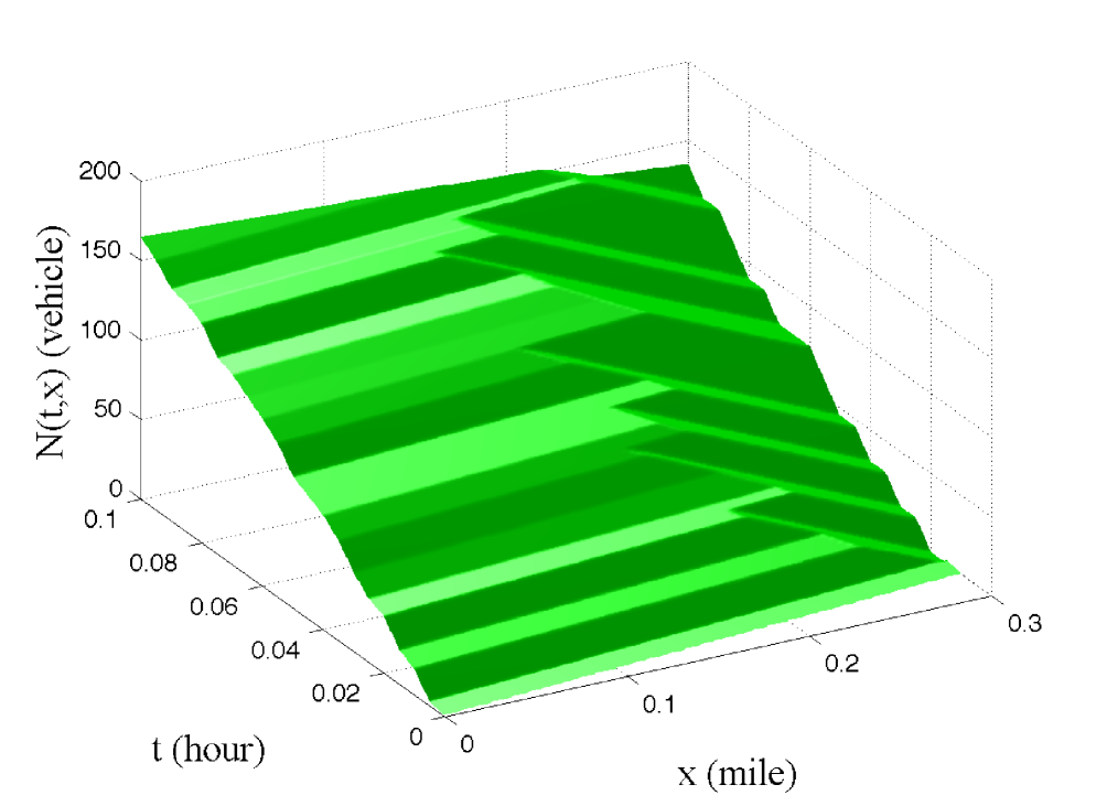
Figure 4: Moskowitz function for link $I_{3}$.

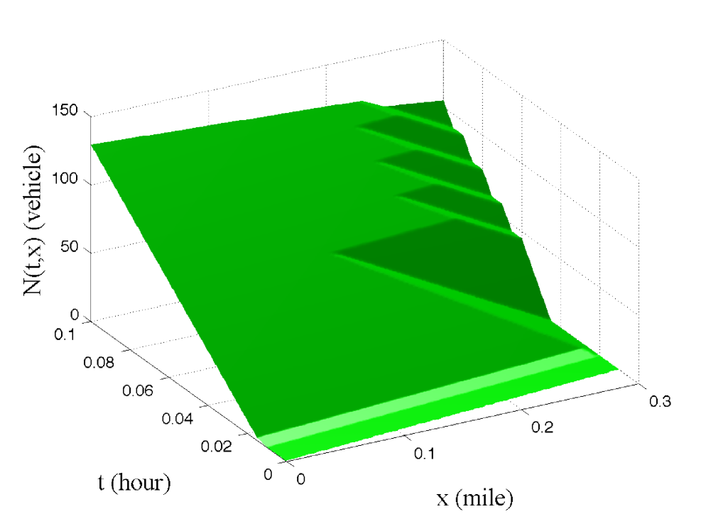
Figure 5: Moskowitz function for link $I_{4}$.

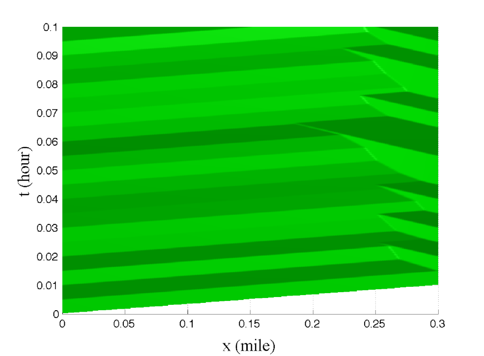
Figure 6: Moskowitz function for link $I_{1}$.

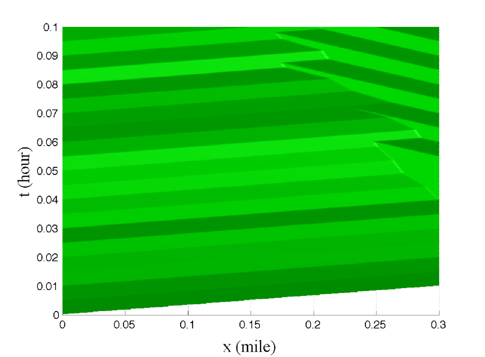
Figure 7: Moskowitz function for link $I_{2}$.

5 Conclusion

This paper proposes a link-based signal control problem. The key ingredient of our formulation is the use of the Lax-Hopf formula to detect latent shocks and hence to identity the regimes (free flow/congested) at the entrance and exit of each link. The analytical framework allows us to further bound the congested region and to avoid spillback. The problem of adaptive signal control is formulated in discrete time as a mixed integer linear program. The resulting MILP requires fewer (binary) variables compared to cell-based approaches.

One limitation of the current approach is the lack of computational tractability, when the problem size scales up. Future research aims at exploring heuristic optimization algorithms such as the genetic algorithms; and new computational paradigms involving parallel computing.

References

- Aubin et al., (2008) Aubin, J.P., Bayen, A.M., Saint-Pierre, P., 2008. Dirichlet problems for some Hamilton-Jacobi equations with inequality constraints. SIAM Journal on Control and Optimization 47 (5), 2348-2380.
- Bressan, (2000) Bressan, A., 2000. Hyperbolic Systems of Conservation Laws. The One Dimensional Cauchy Problem. Oxford University Press.
- (3) Bressan, A., Han, K., 2011a. Optima and equilibria for a model of traffic flow. SIAM Journal on Mathematical Analysis 43 (5), 2384-2417.
- (4) Bressan, A., Han, K., 2011b. Nash equilibria for a model of traffic flow with several groups of drivers. ESAIM: Control, Optimization and Calculus of Variations, doi:10.1051/cocv/2011198.
- Bretti et al., (2006) Bretti, G., Natalini, R., Piccoli, B., 2006. Numerical approximations of a traffic flow model on networks, Networks and Heterogeneous Media 1, 57-84.
- Claudel and Bayen, (2010) Claudel, C.G., Bayen, A.M., 2010. Lax-Hopf based incorporation of internal boundary conditions into Hamilton-Jacobi equation. Part I: Theory. IEEE Transactions on Automatic Control 55 (5), 1142-1157.
- Coclite et al., (2005) Coclite, G.M., Garavello, M., Piccoli, B., 2005. Traffic flow on a road network, SIAM Journal on Mathematical Analysis 36 (6), 1862-1886.
- Daganzo, (1994) Daganzo, C.F., 1994. The cell transmission model. Part I: A simple dynamic representation of highway traffic. Transportation Research Part B 28 (4), 269-287.
- Daganzo, (1995) Daganzo, C.F., 1995. The cell transmission model. Part II: Network traffic. Transportation Research Part B 29 (2), 79-93.
- Daganzo, (2005) Daganzo, C.F., 2005. A variational formulation of kinematic waves: basic theory and complex boundary conditions. Transportation Research Part B 39 (2), 187-196.
- Evans, (2010) Evans, L.C., 2010. Partial Differential Equations, edition. American Mathematical Society, Providence, RI.
- Friesz et al., (2012) Friesz, T.L., Han, K., Neto, P.A., Meimand, A., Yao, T., 2012. Dynamic user equilibrium based on a hydrodynamic model. Transportation Research Part B, doi:10.1016/j.trb.2012.10.001.
- Garavello and Piccoli, (2006) Garavello, M., Piccoli, B., 2006. Traffic Flow on Networks. Conservation Laws Models. AIMS Series on Applied Mathematics, Springfield, Mo..
- Gartner, (1983) Gartner, N.H., 1983. OPAC: a demand-responsive strategy for traffic signal control. Transportation Research Record 906, 75-81.
- Godunov, (1959) Godunov, S.K., 1959. A difference scheme for numerical solution of discontinuous solution of hydrodynamic equations. Math Sbornik 47 (3), 271-306.
- Han et al., (2012) Han, K., Piccoli, B., Friesz, T.L., Yao, T., 2012. A continuous-time link-based kinematic wave model for dynamic traffic networks. arXiv:1208.5141v1.
- Herty and Klar, (2003) Herty, M., Klar, A., 2003. Modeling, simulation, and optimization of traffic flow networks, SIAM Journal on Scientific Computing 25, 1066-1087.
- Holden and Risebro, (1995) Holden, H., Risebro, N.H., 1995. A mathematical model of traffic flow on a network of unidirectional roads, SIAM Journal on Mathematical Analysis 26 (4), 999-1017.
- Hunt et al., (1982) Hunt, P.B., Robertson, D.I., Bretherton, R.D., Royle, M.C., 1982. The scoot on-line traffic signal optimisation technique. Traffic Engineering and Control 23 (4), 190-192.
- Improta and Cantarella, (1984) Improta, G., Cantarella, G.E., 1984. Control system design for an individual signalized junction. Transportation Research Part B 18 (2), 147-167.
- Jin, (2010) Jin, W.-L., 2010. Continuous kinematic wave models of merging traffic flow. Transportation Research Part B 44, 1084-1103.
- Jin and Zhang, (2003) Jin, W.-L., Zhang, H.M., 2003. On the distribution schemes for determining flows through a merge. Transportation Research Part B 37 (6), 521-540.
- Lax, (1957) Lax, P.D., 1957. Hyperbolic systems of conservation laws II. Communications on Pure and Applied Mathematics 10 (4), 537-566.
- Lax, (1973) Lax, P.D., 1973. Hyperbolic systems of conservation laws and the mathematical theory of shock waves, SIAM.
- Lebacque and Khoshyaran, (1999) Lebacque, J., Khoshyaran, M., 1999. Modeling vehicular traffic flow on networks using macroscopic models, in Finite Volumes for Complex Applications II, 551-558, Hermes Sci. Publ., Paris, 1999.
- Lebacque and Khoshyaran, (2002) Lebacque, J., Khoshyaran, M., 2002. First order macroscopic traffic flow models for networks in the context of dynamic assignment, Transportation Planning State of the Art, M. Patriksson and K. A. P. M. Labbe, eds., Kluwer Academic Publushers, Norwell, MA.
- LeFloch, (1988) Le Floch, P., 1988. Explicit formula for scalar non-linear conservation laws with boundary condition. Mathematical Models and Methods in Applied Sciences 10 (3), 265-287.
- LeVeque, (1992) LeVeque, R.J., 1992. Numerical Methods for Conservation Laws. Birkhäuser.
- Lighthill and Whitham, (1955) Lighthill, M., Whitham, G., 1955. On kinematic waves. II. A theory of traffic flow on long crowded roads. In Proceedings of the Royal Society of London: Series A 229, 317- 345.
- Lin and Wang, (2004) Lin, W.H., Wang, C., 2004. An enhanced 0 - 1 mixed-integer LP formulation for traffic signal control. IEEE Transactions on Intelligent transportation systems 5 (4), 238-245.
- (31) Lo, H., 1999a. A dynamic traffic assignment formulation that encapsulates the cell-transmission model. In Proceedings of the 14th International Symposium on Transportation and Traffic Theory, 327-350.
- (32) Lo, H., 1999b. A novel traffic signal control formulation. Transportation Research Part A 33 (6), 433-448.
- (33) Lo, H., 1999c. A cell-based traffic control formulation: strategies and benefits of dynamic timing plans. Transportation Science 35 (2), 148-164.
- Moskowitz, (1965) Moskowitz, K., 1965. Discussion of ‘freeway level of service as influenced by volume and capacity characteristics’ by D.R. Drew and C.J. Keese. Highway Research Record, 99, 43-44.
- Newell, (1993) Newell, G.F., 1993. A simplified theory of kinematic waves in highway traffic, part I: General theory. Transportation Research Part B 27 (4), 281-287.
- Mirchandani and Head, (2000) Mirchandani, P., Head, L., 2000. A real-time traffic signal control system: architecture, algorithms, and analysis. Transportation Research Part C 9 (6), 415-432.
- Richards, (1956) Richards, P.I., 1956. Shockwaves on the highway. Operations Research 4, 42-51.
- Shen et al., (2007) Shen, W., Nie, Y., Zhang, H.M., 2007. Dynamic network simplex method for designing emergency evacuation plans. Transportation Research Record 2022, 83-93.
- Sims and Dobinson, (1980) Sims, A.G., Dobinson, K.W., 1980. The Sydney coordinated adaptive traffic (SCAT) system philosophy and benefits. IEEE Transactions on Vehicular Technology 29 (2), 130-137.
- Yperman et al., (2005) Yperman, I., S. Logghe and L. Immers, 2005. The Link Transmission Model: An Efficient Implementation of the Kinematic Wave Theory in Traffic Networks, Advanced OR and AI Methods in Transportation, Proc. 10th EWGT Meeting and 16th Mini-EURO Conference, Poznan, Poland, 122-127, Publishing House of Poznan University of Technology.