Visiting All Sites with Your Dog

Abstract

Given a polygonal curve $P$, a pointset $S$, and an $\varepsilon>0$, we study the problem of finding a polygonal curve $Q$ whose vertices are from $S$ and has a Fréchet distance less or equal to $\varepsilon$ to curve $P$. In this problem, $Q$ must visit every point in $S$ and we are allowed to reuse points of pointset in building $Q$. First, we show that this problem in NP-Complete. Then, we present a polynomial time algorithm for a special cases of this problem, when $P$ is a convex polygon.

1 Introduction

Geometric pattern matching and recognition has many applications in geographic information systems, computer aided design, molecular biology, computer vision, traffic control, medical imaging etc. Usually these patterns consist of line segments and polygonal curves. Fréchet metric is one of the most popular ways to measure the similarity of two curves. An intuitive way to illustrate the Fréchet distance is as follows. Imagine a person walking his/her dog, where the person and the dog, each travels a pre-specified curve, from beginning to the end, without ever letting go off the leash or backtracking. The Fréchet distance between the two curves is the minimal length of a leash which is necessary. The leash length determines how similar the two curves are to each other: a short leash means the curves are similar, and a long leash means that the curves are different from each other.

Two problem instances naturally arise: decision and optimization. In the decision problem, one wants to decide whether two polygonal curves $P$ and $Q$ are within $\varepsilon$ Fréchet distance to each other, i.e., if a leash of given length $\varepsilon$ suffices. In the optimization problem, one wants to determine the minimum such $\varepsilon$. In [1], Alt and Godau gave an $O(n^{2})$ algorithm for the decision problem, where $n$ is the total number of segments in the curves. They also solved the corresponding optimization problem in $O(n^{2}\log n)$ time.

In this paper, we address the following variant of the Fréchet distance problem. Consider a point set $S\subseteq\mathbb{R}^{d}$ and a polygonal curve $P$ in $\mathbb{R}^{d}$, for $d\geqslant 2$ being a fixed dimension. The objective is to decide whether there exists a polygonal curve $Q$ within an $\varepsilon$-Fréchet distance to $P$ such that the vertices of $Q$ are all chosen from the pointset $S$. Curve $Q$ has to visit every point of $S$ and it can reuse points. We show that this problem is NP-Complete. We then present a polynomial time decision algorithm for a special case of the problem where the input curve $P$ is a convex polygon.

This paper is organized as follows: in Section 2, we establish our NP-Complete proof for the general case of the problem. In Section 3, we investigate the special case of the problem. Finally, we conclude in Section 4 with some open problems.

2 General Case is NP-Complete

2.1 Preliminaries

Given two curves $\alpha,\beta:[0,1]\rightarrow\mathbb{R}^{d}$, the Fréchet distance between $\alpha$ and $\beta$ is defined as $\delta_{F}(\alpha,\beta)=\inf_{\sigma,\tau}\max_{t\in[0,1]}\|\alpha(\sigma(t)),\beta(\tau(t))\|,$ where $\sigma$ and $\tau$ range over all strictly monotone increasing continuous functions. The following two observations are immediate.

Observation 1.

Given four points $a,b,c,d\in\mathbb{R}^{d}$, if $\|ab\|\leqslant\varepsilon$ and $\|cd\|\leqslant\varepsilon$, then $\delta_{F}(\overrightarrow{ac},\overrightarrow{bd})\leqslant\varepsilon$.

Observation 2.

Let $\alpha_{1}$, $\alpha_{2}$, $\beta_{1}$, and $\beta_{2}$ be four curves such that $\delta_{F}(\alpha_{1},\beta_{1})\leqslant\varepsilon$ and $\delta_{F}(\alpha_{2},\beta_{2})\leqslant\varepsilon$. If the ending point of $\alpha_{1}$ (resp., $\beta_{1}$), is the same as the starting point of $\alpha_{2}$ (resp., $\beta_{2}$), then $\delta_{F}(\alpha_{1}+\alpha_{2},\beta_{1}+\beta_{2})\leqslant\varepsilon$, where $+$ denotes the concatenation of two curves.

Notations. We denote by $P=<p_{1}p_{2}p_{3}...p_{n}>$, a polygonal curve $P$ with vertices $p_{1}p_{2}\dots p_{n}$ in order and by $start(P)$ and $end(P)$, we denote the starting and ending point of $P$, respectively. For a curve $P$ and a point $x$, by $P\oplus x$, we mean connecting $end(P)$ to point $x$ (we use the same notation $P\oplus Q$ to show the concatenation of two curves $P$ and $Q$). Let $M({\overline{ab}})$ denote the midpoint of the line segment ${\overline{ab}}$. For a point $q$ in the plane, let $x(q)$ and $y(q)$ denote the $x$ and $y$ coordinate of $q$, respectively.

For two line segments ${\overline{ab}}$ and ${\overline{cd}}$, with ${\overline{ab}}\dashv{\overline{cd}}$, we denote the intersection point of them. Also, for a point $a$ and a line segment ${\overline{bc}}$, $a\perp{\overline{bc}}$ denotes the point on ${\overline{bc}}$ located on the perpendicular from $a$ to ${\overline{bc}}$. Also, $dist(a,{\overline{bc}})$ denotes the distance between $a$ and segment ${\overline{bc}}$.

Definition 2.1.

Given a pointset $S$ in the plane, let $Curves(S)$ be a set of polygonal curves $Q=<q_{1}q_{2}\dots q_{n}>$ where:

$$\forall{q_{i}}:q_{i}\in S\mbox{ and }$$

$$\forall{a}\in S:\exists{q_{i}}\mbox{ s.t. }q_{i}=a\mbox{ }$$

Definition 2.2.

Given a pointset $S$, a polygonal curve $P$ and a distance $\varepsilon$, a polygonal curve $Q$ is called feasible if: $Q\in Curves(S)$ and $\delta_{F}(P,Q)\leq\varepsilon$.

We show that the problem of deciding whether a feasible curve exists or not is NP-complete. It is easy to see that this problem is in NP, since one can polynomially check whether $Q\in Curves(S)$ and also $\delta_{F}(P,Q)\leq\varepsilon$, using the algorithm in [1].

2.2 Reduction Algorithm

We reduce in Algorithm 1, an instance of 3CNF-SAT formula $\phi$ to an instance of our problem. The input is a boolean formula $\phi$ with $k$ clauses $C_{1},C_{2},\dots,C_{k}$ and $n$ variables $x_{1},x_{2},\dots,x_{n}$ and the output is a pointset $S$, a polygonal curve $P$ in the plane and a distance $\varepsilon=1$.

We construct the pointset $S$ as follows. For each clause $C_{i}$, $1\leq i\leq k$, in the formula $\phi$, we place three points $\{s_{i},g_{i},c_{i}\}$, refereed by $cl_{i}$ points, in the plane, which are computed in the $i$-th iteration of Algorithm 1 (from line 3 to line 13). We define $o_{i}$ to be $M({\overline{{s}_{i}{g}_{i}}})$. By ${{\mathscr{S}}{\mathscr{Q}}}_{i}$, $1\leq i\leq k$, we denote a square in the plane, centered at $o_{i}$, with diagonal ${\overline{{s}_{i}{g}_{i}}}$. We refer to ${{\mathscr{S}}{\mathscr{Q}}}_{i}$, $1\leq i\leq k$, as c-squares. For an example of a pointset $S$ corresponding to a formula, see Figure 1.

Our reduction algorithm constructs the polygonal curve $P$ through $n$ iterations. In the $i$-th iteration, $1\leq i\leq n$, it builds a subcurve ${l}_{i}$ corresponding to a variable $x_{i}$ in the formula $\phi$ and appends that curve to $P$. In addition to those $n$ subcurves, two curves ${l}_{n+1}$ and ${l}_{n+2}$ are appended to $P$. We will later discus the reason we add those two curves to $P$. Every subcurve ${l}_{i}$ of $P$ starts at point $u$ and ends at point $v$. Furthermore, every ${l}_{i}$ goes through c-squares ${{\mathscr{S}}{\mathscr{Q}}}_{1}$ to ${{\mathscr{S}}{\mathscr{Q}}}_{k}$ in order, enters each ${{\mathscr{S}}{\mathscr{Q}}}_{j}$ from the side ${\overline{c_{j}s_{j}}}$ and exists that square from the side ${\overline{c_{j}g_{j}}}$ (for an illustration, see Figure 1). Curve ${l}_{i}$ itself is built incrementally through iterations of the loop at line 29 of Algorithm 1. In the $j$-th iteration, when ${l}_{i}$ goes through ${{\mathscr{S}}{\mathscr{Q}}}_{j}$, three points, which are within ${{\mathscr{S}}{\mathscr{Q}}}_{j}$, are added to ${l}_{i}$ (these three points are computed through lines 30 to 35). Next, before ${l}_{i}$ reaches to ${{\mathscr{S}}{\mathscr{Q}}}_{j+1}$, two points, denoted by $\alpha_{j}$ and $\beta_{j}$, are added to that curve (these two points are computed in lines 37 and 38).

Since each ${l}_{i}$ corresponds to variable $x_{i}$ in our approach, this is how we simulate $1$ or $0$ values of $x_{i}$: Consider a point object ${\mathscr{O}}_{L}$ traversing ${l}_{i}$, from starting point $u$ to ending point $v$. Consider another point object ${\mathscr{O}}_{2}$ which wants to walk from $u$ to $v$ on a path whose vertices are from points in $S$ and it wants to stay in distance one to ${\mathscr{O}}_{L}$. We will show that by our construction, object ${\mathscr{O}}_{2}$ has two options, either taking the path $A=<u,s_{1},g_{2},s_{3}\dots v>$ or the path $B=<u,g_{1},s_{2},g_{3}\dots v>$ (See Figure 1 and 6 for an illustration). Choosing path $A$ by ${\mathscr{O}}_{2}$ means $x_{i}=1$ and choosing path $B$ means $x_{i}=0$. We first prove in Lemma 2.3 that $\delta_{F}({l}_{i},A)\leq 1$ and in Lemma 2.5 that $\delta_{F}({l}_{i},B)\leq 1$. Furthermore, by Lemma 2.7, we prove that that as soon as ${\mathscr{O}}_{2}$ chooses the path $A$ at point $u$ to walk towards $v$, it can not switch to any vertex on path $B$. In addition, in lemmas 2.9 and 2.11, we prove that if $x_{i}$ appears in the clause $C_{j}$, ${\mathscr{O}}_{2}$ could visit point $c_{j}$ via the path $A$ and not $B$. In contrast, when $\neg x_{i}$ appears in the clause $C_{j}$, ${\mathscr{O}}_{2}$ could visit point $c_{j}$ via the path $B$ and not $A$. However, when both of $x_{i}$ and $\neg x_{i}$ does not appear in $C_{j}$, ${\mathscr{O}}_{2}$ can not take $A$ or $B$ to visit $c_{j}$.

Algorithm 1 Reduction Algorithm

0:  3SAT formula $\phi$ with $k$ clauses $C_{1}\dots C_{k}$ and $n$ variables $x_{1}\dots x_{n}$ Construct pointset $S$:

1:  $S\leftarrow\emptyset$

2:  ${g}_{1}=(1,1)$

3:  for $j=1$ to $k$ do

4:      ${s}_{i}\leftarrow\big{(}x({g}_{j})-2,y({g}_{j})-2\big{)}$

5:      $o_{j}{\ \leftarrow\ }M({\overline{{s}_{j}{g}_{j}}})$

6:      if ($j$ is odd)  then

7:           $c_{j}\leftarrow\big{(}x(s_{j}),y({g}_{j})\big{)}$, $w_{j}{\ \leftarrow\ }\big{(}x(o_{j})+\frac{1}{4},y(o_{j})-\frac{1}{4}\big{)}$

8:           ${g}_{j+1}{\ \leftarrow\ }\big{(}x(s_{j})+\frac{1}{4}+8,y(s_{j})+\frac{7}{4}+15\big{)}$

9:      else

10:           $c_{j}\leftarrow\big{(}x(g_{j}),y(s_{j})\big{)}$, $w_{j}{\ \leftarrow\ }\big{(}x(o_{j})-\frac{1}{4},y(o_{j})+\frac{1}{4}\big{)}$

11:           ${g}_{j+1}{\ \leftarrow\ }\big{(}x(s_{j})+\frac{7}{4}+15,y(s_{j})+\frac{1}{4}+8\big{)}$

12:      $z_{j}=M({\overline{c_{j}w_{j}}})$

13:      $S=S\cup\{{s}_{j},{g}_{j},c_{j}\}$

14:  if ($k$ is odd) then

15:      $\eta{\ \leftarrow\ }\big{(}x(o_{k})+1,y(o_{k})+4\big{)}$

16:      $v{\ \leftarrow\ }\big{(}x(o_{k})+1,y(o_{k})+9\big{)}$

17:  else

18:      $\eta{\ \leftarrow\ }\big{(}x(o_{k})+4,y(o_{k})+1\big{)}$

19:      $v{\ \leftarrow\ }\big{(}x(o_{k})+9,y(o_{k})+1\big{)}$

20:  $t{\ \leftarrow\ }\big{(}x(v),y(u)-20\big{)}$

21:  $u=(-9,-1)$

22:  $S=S\cup\{u,v,t\}$ Construct polygonal curve $P$:

23:  $P{\ \leftarrow\ }\emptyset$

24:  $P{\ \leftarrow\ }P\oplus t$

25:  for  $i=1$ to $n+2$  do

26:      ${l}_{i}{\ \leftarrow\ }\emptyset$

27:      ${l}_{i}{\ \leftarrow\ }{l}_{i}\oplus u$

28:      ${l}_{i}{\ \leftarrow\ }{l}_{i}\oplus(-4,-1)$

29:      for $j=1$ to $k$ do

30:           if  ($x_{i}\in C_{j}$ and $j$ is odd ) or ($\neg x_{i}\in C_{j}$ and $j$ is even )  then

31:               ${l}_{i}{\ \leftarrow\ }{l}_{i}\oplus M({\overline{s_{j}c_{j}}})\oplus c_{j}\oplus w_{j}$

32:           else if  ($\neg x_{i}\in C_{j}$ and $j$ is odd ) or ($x_{i}\in C_{j}$ and $j$ is even )  then

33:               ${l}_{i}{\ \leftarrow\ }{l}_{i}\oplus w_{j}\oplus c_{j}\oplus M({\overline{g_{j}c_{j}}})$

34:           else

35:               ${l}_{i}{\ \leftarrow\ }{l}_{i}w_{j}\oplus c_{j}\oplus w_{j}$

36:           if $j\neq k$ then

37:               $\alpha_{j}=\frac{4}{5}g_{j}+\frac{1}{5}g_{j+1}$

38:               $\beta_{j}=\frac{1}{5}s_{j}+\frac{4}{5}s_{j+1}$

39:               ${l}_{i}{\ \leftarrow\ }{l}_{i}\oplus\alpha_{j}\oplus\beta_{j}$

40:      ${l}_{i}{\ \leftarrow\ }{l}_{i}\oplus\eta\oplus v$

41:      $P\leftarrow P\oplus{l}_{i}$

42:      $P{\ \leftarrow\ }P\oplus t$

43:  return  pointset $S$, polygonal curve $P$ and distance $\varepsilon=1$

Lemma 2.3.

Consider any subcurve ${l}_{i}=<u\dots v>$, $1\leq i\leq n+2$, which is built through lines 25 to 40 of Algorithm 1. Let $A$ be the polygonal curve $<u{s}_{1}{g}_{2}{s}_{3}{g}_{4}..v>$. Then, $\delta_{F}({l}_{i},A)\leq 1$.

Proof 2.4.

We prove the lemma by induction on the number of segments along $A$. Consider two point objects ${\mathscr{O}}_{L}$ and ${\mathscr{O}}_{A}$ traversing ${l}_{i}$ and $A$, respectively (Figure 1 depicts an instance of ${l}_{i}$ and $A$). We show that ${\mathscr{O}}_{L}$ and ${\mathscr{O}}_{A}$ can walk their respective curve, from the beginning to end, while keeping distance $1$ to each other.

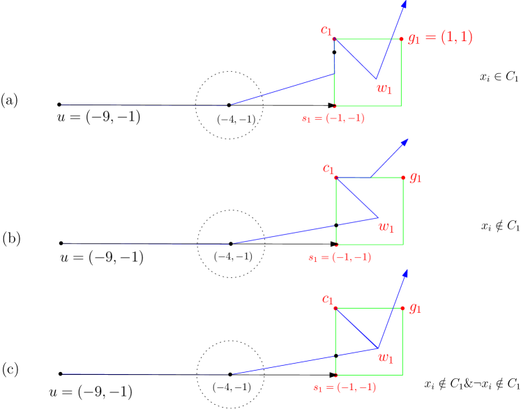
Figure 7: Base case of induction in the proof of Lemma 2.3

The base case of induction trivially holds as follows (see Figure 7 for an illustration): Table 4 lists pairwise location of ${\mathscr{O}}_{L}$ and ${\mathscr{O}}_{A}$, where the distance of each pair is at most $1$. Hence, ${\mathscr{O}}_{A}$ can walk from $u$ to $s_{1}$ on the first segment of $A$ (segment $\overrightarrow{us_{1}}$), while keeping distance $\leq 1$ to ${\mathscr{O}}_{L}$.

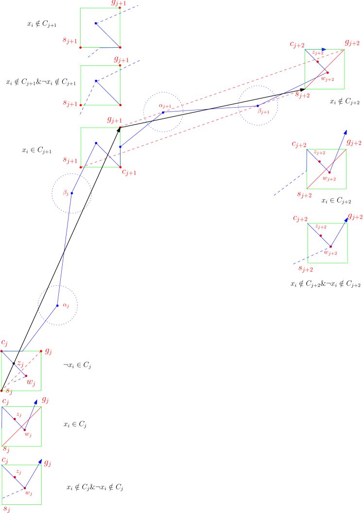
Figure 8: Proof of Lemma 2.3

Assume inductively that ${\mathscr{O}}_{L}$ and ${\mathscr{O}}_{A}$ have feasibly walked along their respective curves, until ${\mathscr{O}}_{A}$ reached $s_{j}$. Then, as the induction step, we show that ${\mathscr{O}}_{A}$ can walk to $g_{j+1}$ and then to $s_{j+2}$ , while keeping distance $1$ to ${\mathscr{O}}_{L}$. Table 1 lists pairwise location of ${\mathscr{O}}_{A}$ and ${\mathscr{O}}_{L}$ such that ${\mathscr{O}}_{A}$ could reach $s_{j+2}$. One can easily check that the distance between pair of points in that table is at most one. (For an illustration, see Figure 8).

	location of ${\mathscr{O}}_{A}$	location of ${\mathscr{O}}_{L}$
if $x_{i}\in C_{j}$	$s_{j}$	$M({\overline{c_{j}s_{j}}})$
	$z_{j}$	$c_{j}$
		$w_{j}$
	${\overline{c_{j}g_{j}}}\dashv{\overline{s_{j}g_{j+1}}}$	${\overline{w_{j}\alpha_{j}}}\dashv{\overline{c_{j}g_{j}}}$
if $\neg x_{i}\in C_{j}$	$s_{j}$	${\overline{\beta_{j-1}w_{j}}}\dashv{\overline{c_{j}s_{j}}}$
	$w_{j}\perp{\overline{s_{j}g_{j+1}}}$	$w_{j}$
	$z_{j}$	$z_{j}$
		$c_{j}$
	${\overline{c_{j}g_{j}}}\dashv{\overline{s_{j}g_{j+1}}}$	$M({\overline{c_{j}g_{j}}})$
if $x_{i}\notin C_{j}\&\neg x_{i}\notin C_{j}$	$s_{j}$	${\overline{\beta_{j-1}w_{j}}}\dashv{\overline{c_{j}s_{j}}}$
	$w_{j}\perp{\overline{s_{j}g_{j+1}}}$	$w_{j}$
	$z_{j}$	$z_{j}$
		$c_{j}$
		$w_{j}$
	${\overline{c_{j}g_{j}}}\dashv{\overline{s_{j}g_{j+1}}}$	${\overline{w_{j}\alpha_{j}}}\dashv{\overline{c_{j}g_{j}}}$
	$h_{1}$ s.t. $\|h_{1}\alpha_{j}\|\leq\varepsilon$	$\alpha_{j}$
	$h_{2}$ s.t. $\|h_{2}\beta_{j}\|\leq\varepsilon$	$\beta_{j}$
if $x_{i}\in C_{j+1}$	${\overline{s_{j+1}c_{j+1}}}\dashv{\overline{s_{j}g_{j+1}}}$	${\overline{\beta_{j}w_{j+1}}}\dashv{\overline{c_{j+1}s_{j+1}}}$
	$z_{j+1}$	$w_{j+1}$
		$z_{j+1}$
		$c_{j+1}$
	$g_{j+1}$	$M({\overline{c_{j+1}g_{j+1}}})$
if $\neg x_{i}\in C_{j+1}$	${\overline{s_{j+1}c_{j+1}}}\dashv{\overline{s_{j}g_{j+1}}}$	$M({\overline{s_{j+1}c_{j+1}}})$
	$z_{j+1}$	$c_{j+1}$
		$w_{j+1}$
	$g_{j+1}$	${\overline{g_{j+1}c_{j+1}}}\dashv{\overline{w_{j+1}\alpha_{j+1}}}$
if $x_{i}\notin C_{j+1}\&\neg x_{i}\notin C_{j+1}$	${\overline{s_{j+1}c_{j+1}}}\dashv{\overline{s_{j}g_{j+1}}}$	${\overline{\beta_{j}w_{j+1}}}\dashv{\overline{c_{j+1}s_{j+1}}}$
	$z_{j+1}$	$w_{j+1}$
		$c_{j+1}$
		$w_{j+1}$
	$g_{j+1}$	${\overline{g_{j+1}c_{j+1}}}\dashv{\overline{w_{j+1}\alpha_{j+1}}}$
	$h_{3}$ s.t. $\|h_{3}\alpha_{j+1}\|\leq\varepsilon$	$\alpha_{j+1}$
	$h_{4}$ s.t. $\|h_{4}\beta_{j+1}\|\leq\varepsilon$	$\beta_{j+1}$
if $\neg x_{i}\in C_{j+2}$	$s_{j+2}$	$\overrightarrow{\alpha_{j+1}w_{j+2}}\dashv{\overline{c_{j+2}s_{j+2}}}$
if $x_{i}\in C_{j+2}$	$s_{j+2}$	$M({\overline{c_{j+2}s_{j+2}}})$
if $x_{i}\notin C_{j+2}\&\neg x_{i}\notin C_{j+2}$	$s_{j+2}$	$\overrightarrow{\alpha_{j+1}w_{j+2}}\dashv{\overline{c_{j+2}s_{j+2}}}$

Table 1: Distance between pair of points is less or equal to one

Finally, if $k$ is an odd number, then $\overrightarrow{s_{k}v}$ is the last segment along $B$, otherwise, $\overrightarrow{g_{k}v}$ is the last one. In any case, that edge crosses the circle ${\mathscr{B}}(\eta,1)$, where $\eta$ is the last vertex of ${l}_{i}$ before $v$ (point $\eta$ is computed in line 14 of Algorithm 1). Therefore, ${\mathscr{O}}_{A}$ can walk to $v$, while keeping distance $1$ to ${\mathscr{O}}_{L}$.

∎

Figure 1: Assume that formula $\phi$ has four clauses $C_{1},C_{2},C_{3}$ and $C_{4}$, where the occurrence of variable $x_{i}$ in those clauses is: $\neg x_{i}\in C_{1}$, $\neg x_{i}\in C_{2}$, $x_{i}\in C_{3}$ and $x_{i}\in C_{4}$. For each clause $C_{i}$, the reduction algorithm places three point $s_{i},g_{i}$ and $c_{i}$ in the plane. Blue curve is an example of curve ${l}_{i}$ which corresponds to variable $x_{i}$ in $\phi$. Red curve is curve $A$.

Lemma 2.5.

Consider any subcurve ${l}_{i}=<u,...,v>$, $1\leq i\leq n+2$, constructed through lines 25 to 40 of Algorithm 1. Let $B$ be the polygonal curve $<u{g}_{1}{s}_{2}{g}_{3}{s}_{4}..v>$. Then, $\delta_{F}({l}_{i},B)\leq 1$.

Proof 2.6.

The proof is analogous to the proof of Lemma 2.3, see appendix.

Lemma 2.7.

Consider any curve ${l}_{i}\subset P$, $1\leq i\leq n+2$, and a point object ${\mathscr{O}}_{L}$ walking from $u$ to $v$ on ${l}_{i}$. Also, imagine two point objects ${\mathscr{O}}_{A}$ and ${\mathscr{O}}_{B}$, walking on curves $A$ and $B$ (from Lemmas 2.3 and 2.5), respectively while keeping distance $1$ to ${\mathscr{O}}_{L}$. Then, if ${\mathscr{O}}_{A}$ switches to path $B$ or ${\mathscr{O}}_{B}$ switches to path $A$, they loose distance $1$ to ${\mathscr{O}}_{L}$.

Proof 2.8.

See Appendix.

For $1\leq i\leq k$, if $i$ is an odd number, set $a_{i}={s}_{i}$ and $b_{i}={g}_{i}$ and if $i$ is an even number, set $a_{i}={g}_{i}$ and $b_{i}={s}_{i}$.

Lemma 2.9.

Consider the curve $A=<ua_{1}a_{2}a_{3}\dots a_{k}v>$ from Lemma 2.3. Let $A_{1}$ be a subcurve of $A$ which starts at $u$ and ends at $a_{j}$, $1\leq j\leq k$. Furthermore, let $A_{2}$ be a subcurve of $A$ which starts at $a_{j}$ and ends at $v$. For any curve ${l}_{i}$ , $1\leq i\leq n+2$, if $x_{i}\in C_{j}$, $\delta_{F}(A_{1}\oplus c_{j}\oplus A_{2},{l}_{i})\leq\varepsilon$. Similarly, consider the curve $B=<ub_{1}b_{2}b_{3}\dots b_{k}v>$ from Lemma 2.5. Let $B_{1}$ be a subcurve of $B$ which starts at $u$ and ends at $b_{j}$, $1\leq j\leq k$. Furthermore, let $B_{2}$ be a subcurve of $B$ which starts at $b_{j}$ and ends at $v$. For any curve ${l}_{i}$ , $1\leq i\leq n+2$, if $\neg x_{i}\in C_{j}$, $\delta_{F}(B_{1}\oplus c_{j}\oplus B_{2},{l}_{i})\leq\varepsilon$.

Proof 2.10.

When $x_{i}$ appears in clause $C_{j}$, point $z=M({\overline{c_{j}a_{j}}})$ is a vertex of ${l}_{i}$. Since $\|c_{j}a_{j}\|=2$ and $z$ is the midpoint of ${\overline{c_{j}a_{j}}}$, ${\mathscr{O}}_{L}$ can wait at $z$ while ${\mathscr{O}}_{A}$ visits $c_{j}$ When $\neg x_{i}$ appears in clause $C_{j}$, point $z=M({\overline{c_{j}b_{j}}})$ is a vertex of ${l}_{i}$. Since $\|c_{j}b_{j}\|=2$ and $z$ is the midpoint of ${\overline{c_{j}b_{j}}}$, ${\mathscr{O}}_{L}$ can wait at $z$ while ${\mathscr{O}}_{A}$ visits $c_{j}$ and comes back to $b_{j}$

Lemma 2.11.

Consider curve $A$ (respectively, $B$). For any curve ${l}_{i}$, $1\leq i\leq n+2$, if $x_{i}\notin C_{j}$ and $\neg x_{i}\notin C_{j}$, then $A$ (resp., $B$) can not be modified to visit $c_{j}$.

Proof 2.12.

This is because $dist(w_{j},{\overline{a_{j}c_{j}}})>1$ and $dist(w_{j},{\overline{b_{j}c_{j}}})>1$.

Theorem 2.13.

Given a formula $\phi$ with $k$ clauses $C_{1},C_{2},\dots,C_{k}$ and $n$ variables $x_{1},x_{2}\dots,x_{n}$, as input let curve $P$ and pointset $S$ be the output of Algorithm 1. Then, $\phi$ is satisfiable iff a curve $Q\in Curves(S)$ exists such that $\delta_{F}(P,Q)\leq 1$.

Proof 2.14.

For $(\Rightarrow)$: Assume that formula $\phi$ is satisfied. In Algorithm 2, we show that knowing the truth value of the literals in $\phi$, we can build a curve $Q$ which visits every point in $S$ and $\delta_{F}(P,Q)\leq 1$.

Algorithm 2 Build a feasible curve $Q$

0:  Truth table of variables $x_{1},x_{2},\dots,x_{n}$ in $\phi$

1:  $Q{\ \leftarrow\ }\emptyset$

2:  $Q{\ \leftarrow\ }Q\oplus t$

3:  for $i=1$ to $n$ do

4:      if $(x_{i}=1)$ then

5:           $\pi{\ \leftarrow\ }<ua_{1}a_{2}a_{3}\dots a_{k}v>$

6:           for all $C_{j}$ clauses, if $x_{i}\in C_{j}$  do

7:               let $\pi_{1}$ be subcurve of $\pi$ from $u$ to $a_{j}$

8:               let $\pi_{2}$ be subcurve of $\pi$ from $a_{j}$ to $v$

9:               $\pi{\ \leftarrow\ }\pi_{1}\oplus c_{j}\oplus\pi_{2}$

10:           $Q{\ \leftarrow\ }Q\oplus\pi$

11:      else

12:           $\pi{\ \leftarrow\ }<ub_{1}b_{2}b_{3}\dots b_{k}v>$

13:           for all $C_{j}$ clauses, if $\neg x_{i}\in C_{j}$  do

14:               let $\pi_{1}$ be subcurve of $\pi$ from $u$ to $b_{j}$

15:               let $\pi_{2}$ be subcurve of $\pi$ from $b_{j}$ to $v$

16:               $\pi{\ \leftarrow\ }\pi_{1}\oplus c_{j}\oplus\pi_{2}$

17:           $Q{\ \leftarrow\ }Q\oplus\pi$

18:      $Q{\ \leftarrow\ }Q\oplus t$

19:  $Q{\ \leftarrow\ }Q\oplus<ua_{1}a_{2}a_{3}\dots a_{k}v>$

20:  $Q{\ \leftarrow\ }Q\oplus t$

21:  $Q{\ \leftarrow\ }Q\oplus<ub_{1}b_{2}b_{3}\dots b_{k}v>$

22:  $Q{\ \leftarrow\ }Q\oplus t$

23:  return Q

First we show $\delta_{F}(P,Q)\leq 1$, where $Q$ is the output curve of Algorithm 2. Recall that by Algorithm 1, curve $P$ includes $n$ subcurves ${l}_{i}$ each corresponds to a variable $x_{i}$. Both curves $P$ and $Q$ start and end at a same point $t$. For each curve $\pi$ which is appended to $Q$ in the $i$-th iteration of Algorithm 2 (line 10 or line 17), $\delta_{F}(\pi,{l}_{i})\leq 1$ by Lemma 2.9. Notice that $P$ also includes two additional subcurves ${l}_{n+1}$ and ${l}_{n+2}$ whereas there is no variable $x_{n+1}$ and $x_{n+2}$ in formula $\phi$. These two curves are to resolve two special cases: when all variables $x_{i}$ are 1, no $\neg x_{i}$ appears in $\phi$, and when all variables $x_{i}$ are 0, no $x_{i}$ appears in $\phi$. Because of these two curves, we add two additional curves in line 19 and 21 to $Q$. Finally, by Observation 2, $\delta_{F}(P,Q)\leq 1$.

Next, we show that curve $Q$ visits every point in $S$. First of all, by the curves added to $Q$ in line 19 and 21, all $a_{j}$ and $b_{j}$, $1\leq j\leq k$, in $S$ will be visited. It is sufficient to show that $Q$ will visit all $c_{j}$ points in $S$ as well. Since formula $\phi$ is satisfied, every clause $C_{i}$ in $\phi$ must be satisfied too. Fix clause $C_{j}$. At least one of the literals in $C_{j}$ must have a truth value $1$. If $x_{i}\in C_{j}$ and $x_{i}=1$, then by line 9, curve $Q$ visits $c_{j}$. On the other hand, if $\neg x_{i}\in C_{j}$ and $x_{i}=0$, by line 16, curve $Q$ visits $c_{j}$. We conclude that curve $Q$ is feasible.

Now we prove the $(\Leftarrow)$ part:

Let $Q$ be a feasible curve with respect to $P$ and pointset $S$. Notice that curve $P$ consists of $n$ subcurve ${l}_{i}$, $1\leq i\leq n$, each corresponds to one variable $x_{i}$. From the configuration of each ${l}_{i}$ in c-squares, one can easily construct formula $\phi$ with all of its clauses and literals.

Imagine two point objects ${\mathscr{O}}_{Q}$ and ${\mathscr{O}}_{P}$ walk on $P$ and $Q$ respectively. We find the truth value of variable $x_{i}$ in the formula by looking at the path that ${\mathscr{O}}_{Q}$ takes to stay in $1$-Fréchet distance to ${\mathscr{O}}_{P}$, when ${\mathscr{O}}_{P}$ walks on curve ${l}_{i}$ corresponding to $x_{i}$. If ${\mathscr{O}}_{Q}$ takes path $A$ from Lemma 2.3 while ${\mathscr{O}}_{P}$ is walking on ${l}_{i}$, then $x_{i}=1$; whereas If ${\mathscr{O}}_{Q}$ takes path $B$ from Lemma 2.5 while ${\mathscr{O}}_{P}$ is walking on ${l}_{i}$, then $x_{i}=0$. Object ${\mathscr{O}}_{Q}$ decides between path $A$ or $B$, , when both ${\mathscr{O}}_{Q}$ and ${\mathscr{O}}_{P}$ are at point $u$. Lemma 2.7 ensures that once they start walking, ${\mathscr{O}}_{Q}$ can not change its path from $A$ to $B$ or from $B$ to $A$. Therefore, the truth value of a variable $x_{i}$ is consistent.

The only thing left to show is the reason that formula $\phi$ is satisfiable. It is sufficient to show every clause of $\phi$ is satisfiable. Consider any clause $C_{j}$. Since curve $Q$ is feasible, it uses every point in $S$. Assume w.l.o.g. that ${\mathscr{O}}_{Q}$ visits $c_{j}$ when ${\mathscr{O}}_{P}$ is walking along curve ${l}_{i}$. By Lemmas 2.7 and 2.9, this only happens when either ($x_{i}$ appears in $C_{i}$ and $x_{i}=1$) or ($\neg x_{i}$ appears in $C_{i}$ and $x_{i}=0$). Therefore, $C_{j}$ is satisfiable.

The last ingredient of the NP-completeness proof is to show that the reduction takes polynomial time. One can easily see that Algorithm 1 has running time $O(nk)$, where $n$ is the number of variables in the input formula with $k$ clauses.

To show the correctness of above lemmas, we have implemented our reduction algorithm. We test our algorithm on a formula $\phi$ with four clauses. This enables us to check all possible configurations of ${l}_{i}$ in Algorithm 1. The program generates three sets, a pointset $S=\{s_{1},g_{1},c_{1},s_{2},g_{2},c_{2},s_{3},g_{3},c_{3},s_{4},g_{4},c_{4}\}$, a curve set $L$ and a curve set $C$ as follows.

Imagine a polygonal curve which starts from point $u$, goes through points in $S$ and ends at $v$. Our program generates all possible such curves and keep them in set $C$. Therefore, $C$ contains almost 1,000,000,000 curves.

Another set $L$ includes all different configuration of curve ${l}_{i}$ which corresponds to variable $x_{i}$ in the formula. Since $x_{i}$ or $\neg x_{i}$ or none could appear in one clause and the formula has four clauses, the set $L$ contains 81 different curves.

In our application, we compute Fréchet distance between every curve in $C$ and every curve in $L$. The results show that all the curves in $C$ have Fréchet distance greater than $1$ to curves in $L$ except two curves $<u,s_{1},g_{2},s_{3},g_{4},v>$ and $<u,g_{1},s_{2},g_{3},s_{4},v>$. In other words, for only 162 pairs of curves, we got:

$\forall\mu\in L:\delta_{F}(\mu,<u,s_{1},g_{2},s_{3},g_{4},v>)\leq 1$ and $\forall\mu\in L:\delta_{F}(\mu,<u,g_{1},s_{2},g_{3},s_{4},v>)\leq 1$

In addition to above tests, we verified the correctness of Lemma 2.9 in different cases.

3 Convex Polygon Case

In this section, we address the following problem: given a convex polygon ${\mathscr{P}}$ and a pointset $S$ in the plane, find a polygonal curve $Q$ whose vertices are from $S$, and the Fréchet distance between $Q$ and a boundary curve of ${\mathscr{P}}$ is minimum. Note that each point of $S$ must be used in $Q$ and it can be used more than once. In the decision version of the problem, we want to decide if there is a polygonal curve $Q$ through all points in $S$, whose Fréchet distance to a polygon’s boundary curve is at most $\varepsilon$, for a given $\varepsilon\geqslant 0$.

3.1 Preliminaries

We borrow some notations from [2] as we make use of the algorithm in that paper to solve the decision version of our problem. For any point $p$ in the plane, we define ${\mathscr{B}}(p,\varepsilon)\equiv\{q\in\mathbb{R}^{2}:\|pq\|\leqslant\varepsilon\}$ to be a ball of radius $\varepsilon$ centered at $p$, where $\|\cdot\|$ denotes Euclidean distance. Given a line segment $L\subset\mathbb{R}^{2}$, we define ${\mathscr{C}}(L,\varepsilon)\equiv\cup_{p\in L}{\mathscr{B}}(p,\varepsilon)$ to be a cylinder of radius $\varepsilon$ around $L$.

In this section, whenever we say polygon, we mean a convex polygon. Also, when we say a curve visits a point $u$, we mean that $u$ is a vertex of the curve. We denote by ${\mathscr{C}H}(S)$ the convex hull of pointset $S$.

For an interval $I$ of points in $P$, we denote by $\operatorname{left}(I)$ and $\operatorname{right}(I)$ the first and the last point of $I$ along $P$, respectively. Given two points $u$ and $v$ in $S_{i}$, we say $u$ is before $v$, and denote it by $u\preceq v$ when $\operatorname{left}(P_{i}[u])$ is located before $\operatorname{left}(P_{i}[v])$ on $P$. Moreover, we say $u$ is entirely before $v$ (or $v$ is entirely after $u$) and denote it by $u\prec v$, when $\operatorname{right}(P_{i}[u])$ is located before $\operatorname{left}(P_{i}[v])$ on $P$.

The Decision Algorithm in [2] Given a polygonal curve $P$ of size $n$ (with starting point $s$ and ending point $t$), a pointset $S$ of size $k$ and a distance $\varepsilon>0$, the algorithm in that paper decides in $O(nk^{2})$ time, whether there exists a polygonal curve through some points in $S$ in $\varepsilon$-Fréchet distance to $P$.

Curve $P$ is composed of $n$ line segments ${P}_{1}\ldots{P}_{n}$. For each segment ${P}_{i}$, $C_{i}$ denotes the cylinder ${\mathscr{C}}({P}_{i},\varepsilon)$, and $S_{i}$ denotes the set $S\cap C_{i}$. Furthermore, for each point $v\in C_{i}$, ${P}_{i}[v]$ denotes the line segment ${P}_{i}\cap{\mathscr{B}}(v,\varepsilon)$ [2]. A polygonal curve $R$ is called semi-feasible if all its vertices are from $S$ and $\delta_{F}(R,P^{\prime})\leqslant\varepsilon$ for a subcurve $P^{\prime}\subseteq P$ starting at $s$. A point $v\in S_{i}$ is called reachable, at cylinder $C_{i}$, if there is a semi-feasible curve ending at $v$ in $C_{i}$.

Following is a brief outline of how the decision algorithm in [2] works: it processes the cylinders one by one from $C_{1}$ to $C_{n}$, and identifies at each cylinder $C_{k}$ all points of $S$ which are reachable at $C_{k}$. The reachable points for each cylinder $C_{k}$, $k$ from 1 to $n$, is maintained in a set called reachability set, denoted by ${\mathscr{R}}_{k}$. In the $k$-th iteration of the algorithm, first all points in $S_{k}$ which are reachable through a point in a set ${\mathscr{R}}_{i}$, for $1\leqslant i<k$, are added to ${\mathscr{R}}_{k}$ . These points are called the entry points of cylinder $C_{k}$. We denote, by ${\lambda_{k}}$, the leftmost entry point of cylinder $C_{k}$, which at this step, equal to $q=\min_{v\in{\mathscr{R}}_{k}}{\operatorname{left}(P_{k}[v])}$. Next, all points in $S_{k}$ which are reachable through ${\lambda_{k}}$ are added to ${\mathscr{R}}_{k}$. Finally, the decision algorithm returns YES , if ${\mathscr{R}}_{n}\cap{\mathscr{B}}(t,\varepsilon)\not=\emptyset$.

Figure 2: A problem instance

3.2 Decision Algorithm

Let ${\mathscr{P}}$ be a convex polygon of size $n$, $S$ be a pointset of size $k$ and $\varepsilon\geq 0$ be an input distance. For ${\mathscr{P}}$, we call a curve, a boundary curve of ${\mathscr{P}}$, denote it by ${\sigma({\mathscr{P}},{u})}$, if it starts from point $u$ on the boundary of ${\mathscr{P}}$, goes around the polygon on the boundary once and ends at $u$.

Definition 3.1.

Given a pointset $S$, a convex polygon ${\mathscr{P}}$ and a distance $\varepsilon$, a polygonal curve $Q$, is called feasible if $Q\in Curves(S)$ and a boundary curve ${\sigma({\mathscr{P}},{z})}$ exists such that $\delta_{F}({\sigma({\mathscr{P}},{z})},Q)\leq\varepsilon$.

As the first step of our algorithm, we execute the decision algorithm in [2]. Note that here as opposed to in [2], the starting and ending point of the curve is unclear because the input is a convex polygon. Which point on the boundary we choose? The following lemma justifies our choice later:

Lemma 3.2.

Given a convex polygon ${\mathscr{P}}$, a pointset $S$ and a distance $\varepsilon$, a necessary condition to have a feasible curve through $S$ is: $\delta_{F}(\sigma({\mathscr{C}H}(S),z),{\sigma({\mathscr{P}},{z^{\prime}})})\leq\varepsilon$, where $z$ is a vertex of ${\mathscr{C}H}(S)$ and $z^{\prime}$ is a point on the boundary of ${\mathscr{P}}$ s.t. $\|zz^{\prime}\|\leq\varepsilon$.

Proof 3.3.

See Appendix.

Let $x$ be the point with smallest $x$-coordinate in $S$ and $x^{\prime}$ be a point on the boundary of ${\mathscr{P}}$ s.t. $\|xx^{\prime}\|\leq\varepsilon$. Furthermore, let $\rho={\sigma({\mathscr{P}},{x^{\prime}})}$ (curve $\rho$ has $n+1$ line segments $\rho_{1},\rho_{2},\dots,\rho_{n+1}$) Run the decision algorithm in [2], with parameters $\rho,S$ and $\varepsilon$. Result is the reachability sets ${\mathscr{R}}_{1},{\mathscr{R}}_{2},\dots,{\mathscr{R}}_{n+1}$ where each ${\mathscr{R}}_{i}$ maintains the reachable points at cylinder $C_{i}$.

Definition 3.4.

Consider two consecutive reachability sets ${\mathscr{R}}_{i}$ and ${\mathscr{R}}_{j}$, $1\leq i<j\leq n$. Let $u$ be a point in ${\mathscr{R}}_{i}$. Then, we call $u$ a type A point at $C_{i}$ if there exists a semi-feasible curve which contains $u$ as its vertex and ends at ${\lambda_{j}}$. Otherwise, we call $u$ a type B point at $C_{i}$ and we call ${\lambda_{j}}$ the rival of $u$.

Observation 3.

Let $u$ and $v$ be type A and type B points at cylinder $C_{i}$, respectively. Then, $u\prec v$.

Observation 4.

A type B point $u$ at cylinder $C_{i}$ is:

• a $B1$ point at $C_{i}$: when $u$ doesn’t reach to ${\lambda_{j}}$ but it reaches to some other point $v$ in ${\mathscr{R}}_{j}$ (see Figure 3a).

• a $B2$ point at $C_{i}$, when $u$ does not reach to any point in ${\mathscr{R}}_{j}$, but it reaches to a point in ${\mathscr{R}}_{k}$, $i<j\leq k$ (see Figure 3b).

• a $B3$ point at $C_{i}$, when $u$ does not reach to any point in ${\mathscr{R}}_{k}$, $i<j\leq k$ (see Figure 3c).

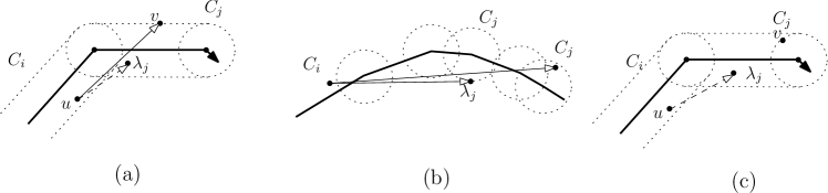
Figure 3: (a) Point $u$ is a $B1$ point at $C_{i}$ (b) Point $u$ is a $B2$ point at $C_{i}$ (c) Point $u$ is a $B3$ point at $C_{i}$.

After running the algorithm in [2], we process the reachability sets ${\mathscr{R}}_{1},{\mathscr{R}}_{2},\dots\mathscr{R}_{n-1}$, one by one in order, and we identify the types of the points for every point in each set. Notice that a point $u$ may be located in multiple cylinders, so it might be reachable at more that one cylinder and thus be in more than one reachability set.

Let $\pi$ and $\mu$ be the upper and the lower chain of ${\mathscr{P}}$, respectively. Let Tube(${\mathscr{P}}$) be the union of all ${\mathscr{C}}({P}_{i},\varepsilon)$, where $P_{i}$ is an edge of ${\mathscr{P}}$, $1\leq i\leq n$. Tube($\pi$) and Tube($\mu$) are defined, analogously.

Definition 3.5.

We call a point a Twice-TypeB point, if it is of type B at two cylinders.

Definition 3.6.

We call a connected area within Tube(${\mathscr{P}}$), shared between two cylinders, one corresponding to an edge in $\pi$ and another corresponding to an edge in $\mu$, a Double-TypeB area, if it contains a Twice-TypeB point.

Lemma 3.7.

Given a polygon ${\mathscr{P}}$, a pointset $S$ and $\epsilon>0$, at most two Double-TypeB areas exists.

Proof 3.8.

Assume w.l.o.g. that ${\mathscr{P}}$ is stretched horizontally (see Figure 4)(In the case that ${\mathscr{P}}$ is vertically stretched, decompose it into right and left chains and the rest of argument is the same as here).

Assume for the sake of contradiction, that there are three such areas and a point $w$ is a Twice-TypeB point located in the middle one. (see Figure 4). Let $w^{\prime}$ and $w^{\prime\prime}$ be the rivals of $w$ in the upper and lower chain of ${\mathscr{P}}$, respectively. Assume w.l.o.g. that $w$ and $w^{\prime}$ are located in two consecutive cylinders (within Tube($\pi$)) which share ${\mathscr{B}}(p_{1},\varepsilon)$. Similarly, assume w.l.o.g. that $w$ and $w^{\prime\prime}$ are located in two consecutive cylinders (within Tube($\mu$)) which share ${\mathscr{B}}(p_{2},\varepsilon)$. Since $w$ is a type B point and $w^{\prime}$ is the rival of $w$, edge $\overrightarrow{ww^{\prime}}$ does not cross circle ${\mathscr{B}}(p_{1},\varepsilon)$. Because of the same reason, edge $\overrightarrow{ww^{\prime\prime}}$ does not cross circle ${\mathscr{B}}(p_{2},\varepsilon)$. This implies that, vertices of ${\mathscr{P}}$ to the right of $p_{1}$ has a $y$-coordinate less than $p_{1}$ and vertices before $p_{2}$ has a $y$-coordinate greater than $p_{2}$, meaning that $p_{2}$ has the lowest $y$ coordinate among vertices of ${\mathscr{P}}$. Therefore, no Double-TypeB area exists to the right of the area in which $w$ is located, a contradiction.

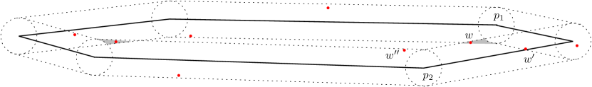
Figure 4: Proof of Lemma 3.7

Lemma 3.9.

There exists a feasible curve iff Algorithm 3 returns YES.

Proof 3.10.

First $(\Leftarrow)$: It is easy to observe that conditions in lines 5, 6, 8 are necessary to have a feasible curve through $S$. It suffices to show for the curve $\alpha$ built by Algorithm 3, $\delta_{F}(\alpha,\rho)\leq\varepsilon$.

We show this by induction on the number of edges in $\rho$. To handle the base case of the induction, assume that $\rho$ has an additional edge consist of only point $x^{\prime}$. Imagine a point object ${\mathscr{O}}_{\mathscr{P}}$ walking on the boundary of ${\mathscr{P}}$, starting from point $x^{\prime}$ and imagine another point object ${\mathscr{O}}_{\alpha}$ walking on curve $\alpha$ starting from $x$ while keeping distance $\leq 1$ to ${\mathscr{O}}_{\mathscr{P}}$. Since distance ${\mathscr{O}}_{\mathscr{P}}$ and ${\mathscr{O}}_{\alpha}$ is less than $\varepsilon$ at the start, the base case of the induction holds.

We show ${\mathscr{O}}_{\mathscr{P}}$ can walk the whole $\rho$ and ends at $x^{\prime}$. Assume inductively that in the loop in line 11, we have processed ${\mathscr{R}}_{1}$ to ${\mathscr{R}}_{n-1}$, and now we are about to process ${\mathscr{R}}_{n}$. So every point in $S_{i-1}$ is in $\alpha$ and ${\mathscr{O}}_{\mathscr{P}}$ can walk to a point in $\rho_{i-1}$ in $\varepsilon$ distance to ${\mathscr{O}}_{\alpha}$. Let $v$ be the leftmost point at $C_{i}$ such that $end(\alpha)\leadsto v$. If $v={\lambda_{i}}$, by Observation 2, we can add every point in $S_{i}$ to $\alpha$ and ${\mathscr{O}}_{\mathscr{P}}$ can proceed to $\rho_{i}$. Otherwise; since ${\lambda_{i}}$ is a reachable point, a point $u$ must exist in ${\mathscr{R}}_{k}$, $k<i$ such that $u$ reach ${\lambda_{i}}$. Assume that $u$ is after all points in direction $\overrightarrow{\rho}$ which can reach to ${\lambda_{i}}$. It suffices to show point $u$ is a vertex of $\alpha$, so that in line 14, by reaching to $u$, the algorithm stops removing vertices in $\alpha$ and connects $u$ to ${\lambda_{i}}$. Two cases happen here: (i) $u\in S_{i-1}$, and some points in $S_{i-1}$ are type A and some are type B points. Then, type B points are removed from $\alpha$ (because they can not reach ${\lambda_{i}}$ by definition), and $u$ will be connected to $\lambda_{i}$ (see Figure 5). Therefore, ${\mathscr{O}}_{\mathscr{P}}$ can walk to the next edge on $\rho$. (ii) When $u\in{\mathscr{R}}_{k}$, $k<i-1$, then observe that because of the convexity of the polygon, $u$ reach points in ${\mathscr{R}}_{j}$ which can not reach ${\lambda_{i}}$, $k<j<i$ (see Figure 5). Therefore, $u$ is a vertex in $\alpha$.

Now we show that curve $\alpha$ can be modified such that it visits every Twice-TypeB point when ${\mathscr{O}}_{\mathscr{P}}$ walks on $\pi$ (with the same argument, curve $\alpha$ can be modified to visit all such points when ${\mathscr{O}}_{\mathscr{P}}$ walks on $\mu$). Let’s call Double-TypeB areas, area I and area II. Let $b$ be the first type B point in direction $\overrightarrow{\pi}$ at area I. Assume w.l.o.g. that $b$ is in $S_{i}$. Let $u$ be a point after all points in direction $\overrightarrow{\pi}$ which can reach ${\lambda_{i+1}}$. Because of the convexity of polygon, point $u$ reaches $b$. It is clear that as soon as $\alpha$ reaches $b$, it can visit all type B points at $C_{i}$ in sorted $\prec$ order. Let $d$ be the leftmost point in $S_{i+1}$ which the last type B point at $C_{i}$ can reach. If $d$ is a vertex of $\alpha$, then $\alpha$ now has all Twice-TypeB points at area I. When $d$ is not a vertex of $\alpha$, because of the convexity of the polygon, still $d$ can be connected to a vertex of $\alpha$ which is reachable from $d$. Therefore, one can modify curve $\alpha$ to visit Twice-TypeB points.

$(\Rightarrow)$: Let $Q$ be a feasible curve through $S$. Assume that there is no Twice-TypeB point among points in $S$. Let $z$ be any point in $S$. Then, by Lemma 3.7, if $z$ lies in both $Tube(\pi)$ and $Tube(\mu)$, then it can be type B only with respect to one of $\pi$ or $\mu$. Assume w.l.o.g, that $z$ is a type B point in the upper chain. Therefore, $z$ is a type A point in the lower chain and it will be visited by $\alpha$. Now, if there are some Twice-TypeB points in $S$, it is easy to show that $z$ will be visited by one of $\beta$ or $\gamma$ curves in our algorithm.

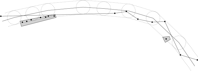
Figure 5: Proof of Lemma 3.9, points in the shaded area can not reach the leftmost entry point of the next non-empty cylinder

Algorithm 3 Decision Algorithm

0:  A convex polygonal ${\mathscr{P}}$, pointset $S$ and distance $\varepsilon$

1:  let $x$ be the point with smallest $x$-coordinate in $S$

2:  let $x^{\prime}$ be a point on the boundary of ${\mathscr{P}}$ s.t. $\|xx^{\prime}\|\leq\varepsilon$

3:  let $\rho={\sigma({\mathscr{P}},{x^{\prime}})}$ (curve $\rho$ has $n+1$ line segments)

4:  run the decision algorithm in [2], with parameters $\rho,S$ and $\varepsilon$

5:  return no if a point in $S$ is not in any ${\mathscr{R}}_{i}$, $1\leq i\leq n+1$

6:  return no if ${\mathscr{R}}_{n+1}\cap{\mathscr{B}}(x^{\prime},\varepsilon)=\emptyset$

7:  process reachability sets from ${\mathscr{R}}_{1}$ to ${\mathscr{R}}_{n}$ in order, to identify types of points in each ${\mathscr{R}}_{i}$

8:  return no if a point exists of type $B3$ in every cylinder at which that point is reachable

9:  $\alpha{\ \leftarrow\ }\emptyset$

10:  $\alpha{\ \leftarrow\ }\alpha\oplus x$

11:  for $i=1$ to $n$  do

12:      let $v$ be a leftmost point at $C_{i}$ s.t. $end(\alpha)\leadsto v$

13:      if  $v\neq{\lambda_{i}}$ then

14:           remove $end(\alpha)$ until a vertex $u$ of $\alpha$ is found s.t. $u\leadsto{\lambda_{i}}$

15:      $\alpha{\ \leftarrow\ }\alpha\oplus$ (every point in $S_{i}$ in sorted $\prec$ order)

16:  if a Twice-TypeB point exists then

17:      $\beta{\ \leftarrow\ }$ modify $\alpha$ s.t. it visits those points in $\pi$

18:      $\gamma{\ \leftarrow\ }$ modify $\alpha$ s.t. it visits those points in $\mu$

19:  return YES if $\alpha$ or $\beta$ or $\gamma$ include all points in $S$

Theorem 3.11.

Given a convex polygon ${\mathscr{P}}$ with $n$ edges and a set $S$ of $k$ points, we can decide in $O(nk^{2})$ time whether there is feasible curve $Q$ through $S$ for a given $\varepsilon\geqslant 0$. Furthermore, a feasible curve $Q$ which minimizing the Fréchet distance to the boundary curve of ${\mathscr{P}}$, can be computed in $O(nk^{2}\log(nk))$ time.

4 Conclusions

In this paper, we investigate the problem of deciding whether a polygonal curve through a given point set $S$ exists which is in $\varepsilon$-Fréchet distance to a given curve $P$. We showed that this problem is NP-Complete. Also, we presented a polynomial time algorithm for the special case of the problem, when a given curve is a convex polygon.

Several open problems arise from our work. From our first result, one could investigate some heuristic methods or approximation algorithms. From the second part, in particular, it is interesting to study the problem in the case where the input is a monotone polygon, a simple polygon or a special type of curve.

Figure 6: Red curve is curve $B$. Blue curve is an example of curve ${l}_{i}$ which corresponds to variable $x_{i}$ in formula $\phi$ with four clauses $C_{1},C_{2},C_{3}$ and $C_{4}$. The occurrence of variable $x_{i}$ in the clauses is: $\neg x_{i}\in C_{1}$, $\neg x_{i}\in C_{2}$, $x_{i}\in C_{3}$ and $x_{i}\in C_{4}$.

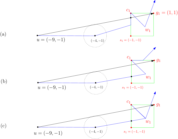
Figure 9: Base case of induction in the proof of Lemma 2.5

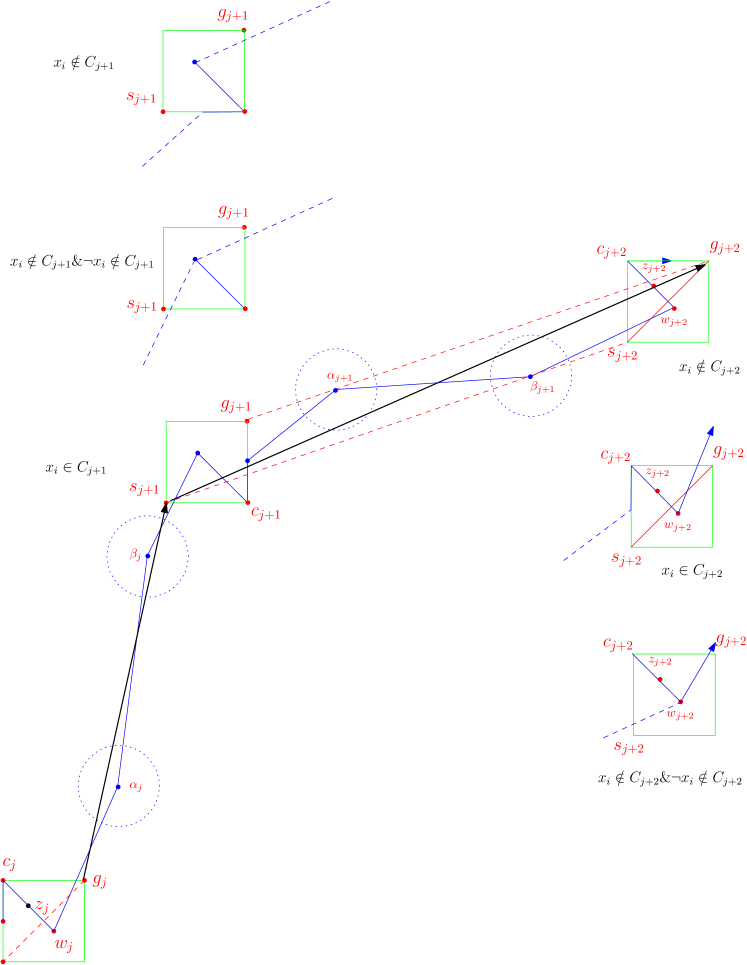
Figure 10: Proof of Lemma 2.5

Proof of Lemma 2.5:

Proof .1.

Consider two point objects ${\mathscr{O}}_{L}$ and ${\mathscr{O}}_{B}$ traversing ${l}_{i}$ and $B$, respectively (Figure 6 depicts an instance of ${l}_{i}$ and $B$). To prove the lemma, we show that ${\mathscr{O}}_{L}$ and ${\mathscr{O}}_{B}$ can walk their respective curves, from beginning to the end, while keeping distance $1$ to each other .

The base case of induction holds as follows (see Figure 9 for an illustration): Table 2 lists pairwise location of ${\mathscr{O}}_{L}$ and ${\mathscr{O}}_{B}$, where the distance of each pair is less or equal to $1$. Therefore, ${\mathscr{O}}_{B}$ can walk from $u$ to $g_{1}$ while keep distance one to ${\mathscr{O}}_{L}$.

if $x_{i}\in C_{1}$	location of ${\mathscr{O}}_{B}$	location of ${\mathscr{O}}_{L}$
	$u$	$u$
	$h_{1}$ s.t. $\|h_{1}\mu_{1}\|\leq\varepsilon$	$\mu_{1}=(-4,-1)$
	$h_{2}=\overrightarrow{ug_{1}}\dashv{\overline{s_{1}c_{1}}}$	$\mu_{2}=M(s_{1}c_{1})$
	$h_{2}$	$c_{1}$
	${\overline{ug_{1}}}\dashv{\overline{c_{1}w_{1}}}$	${\overline{ug_{1}}}\dashv{\overline{c_{1}w_{1}}}$
	$w_{1}\perp ug_{1}$	$w_{1}$
	$g_{1}$	${\overline{w_{1}\alpha_{1}}}\dashv{\overline{c_{1}g_{1}}}$
if $\neg x_{i}\in C_{1}$	$u$	$u$
	$h_{1}$ s.t. $\|h_{1}\mu\|\leq\varepsilon$	$\mu_{1}=(-4,-1)$
	$h_{2}=\overrightarrow{ug_{1}}\dashv{\overline{s_{1}c_{1}}}$	$\mu_{2}=\overrightarrow{\mu_{1}w_{1}}\dashv{\overline{s_{1}c_{1}}}$
	${\overline{ug_{1}}}\dashv{\overline{c_{1}w_{1}}}$	$w_{1}$
		$c_{1}$
	$g_{1}$	$M(c_{1}g_{1})$
if $x_{i}\notin C_{1}\&\neg x_{i}\notin C_{1}$	$u$	$u$
	$h_{1}$ s.t. $\|h_{1}\mu\|\leq\varepsilon$	$\mu_{1}=(-4,-1)$
	$h_{2}=\overrightarrow{ug_{1}}\dashv{\overline{s_{1}c_{1}}}$	$\mu_{2}=\overrightarrow{\mu_{1}w_{1}}\dashv{\overline{s_{1}c_{1}}}$
	${\overline{ug_{1}}}\dashv{\overline{c_{1}w_{1}}}$	$w_{1}$
		$c_{1}$
		$w_{1}$
	$g_{1}$	${\overline{w_{1}\alpha_{1}}}\dashv{\overline{c_{1}g_{1}}}$

Table 2: Pairwise location of ${\mathscr{O}}_{B}$ and ${\mathscr{O}}_{L}$, to prove the base case of induction in Lemma 2.5

Assume inductively that ${\mathscr{O}}_{L}$ and ${\mathscr{O}}_{B}$ have feasibly walked along their respective curves, until ${\mathscr{O}}_{B}$ reached $g_{j}$. Then, as the induction step, we show that ${\mathscr{O}}_{B}$ can walk to $s_{j+1}$ and then to $g_{j+2}$ , while keeping distance $1$ to ${\mathscr{O}}_{L}$. This is shown in Table 3 (see Figure 10 for an illustration).

	location of ${\mathscr{O}}_{B}$	location of ${\mathscr{O}}_{L}$
if $x_{i}\in C_{j}$	$g_{j}$	$\overrightarrow{\alpha_{j-1}w_{j}}\dashv{\overline{c_{j}g_{j}}}$
if $\neg x_{i}\in C_{j}$	$g_{j}$	$M({\overline{c_{j}g_{j}}})$
if $x_{i}\notin C_{j}\&\neg x_{i}\notin C_{j}$	$g_{j}$	$\overrightarrow{\alpha_{j-1}w_{j}}\dashv{\overline{c_{j}g_{j}}}$
	$h_{3}$ s.t. $\|h_{3}\alpha_{j}\|\leq\varepsilon$	$\alpha_{j}$
	$h_{4}$ s.t. $\|h_{4}\beta_{j}\|\leq\varepsilon$	$\beta_{j}$
if $x_{i}\in C_{j+1}$	$s_{j+1}$	${\overline{\beta_{j}w_{j+1}}}\dashv{\overline{c_{j+1}s_{j+1}}}$
	$w_{j+1}\perp{\overline{s_{j+1}g_{j+2}}}$	$w_{j+1}$
	$z_{j+1}$	$z_{j+1}$
	${\overline{g_{j+1}c_{j+1}}}\dashv{\overline{s_{j+1}g_{j+2}}}$	$c_{j+1}$
		$M({\overline{c_{j+1}g_{j+1}}})$
if $\neg x_{i}\in C_{j+1}$	$s_{j+1}$	$M({\overline{s_{j+1}c_{j+1}}})$
	$z_{j+1}$	$c_{j+1}$
		$w_{j+1}$
	${\overline{g_{j+1}c_{j+1}}}\dashv{\overline{s_{j+1}g_{j+2}}}$	${\overline{g_{j+1}c_{j+1}}}\dashv{\overline{w_{j+1}\alpha_{j+1}}}$
if $x_{i}\notin C_{j+1}\&\neg x_{i}\notin C_{j+1}$	$s_{j+1}$	${\overline{\beta_{j}w_{j+1}}}\dashv{\overline{c_{j+1}s_{j+1}}}$
	$z_{j+1}$	$w_{j+1}$
		$c_{j+1}$
		$w_{j+1}$
	${\overline{g_{j+1}c_{j+1}}}\dashv{\overline{s_{j+1}g_{j+2}}}$	${\overline{g_{j+1}c_{j+1}}}\dashv{\overline{w_{j+1}\alpha_{j+1}}}$
	$h_{5}$ s.t. $\|h_{5}\alpha_{j+1}\|\leq\varepsilon$	$\alpha_{j+1}$
	$h_{6}$ s.t. $\|h_{6}\beta_{j+1}\|\leq\varepsilon$	$\beta_{j+1}$
if $x_{i}\in C_{j+2}$	${\overline{s_{j+2}c_{j+2}}}\dashv{\overline{s_{j+1}g_{j+2}}}$	$M({\overline{s_{j+2}c_{j+2}}})$
	$z_{j+2}$	$c_{j+2}$
		$w_{j+2}$
	$g_{j+2}$	${\overline{g_{j+2}c_{j+2}}}\dashv{\overline{w_{j+2}\alpha_{j+2}}}$
if $\neg x_{i}\in C_{j+2}$	${\overline{s_{j+2}c_{j+2}}}\dashv{\overline{s_{j+1}g_{j+2}}}$	${\overline{s_{j+2}c_{j+2}}}\dashv{\overline{\beta_{j+1}w_{j+2}}}$
	$z_{j+2}$	$w_{j+2}$
		$c_{j+2}$
	$g_{j+2}$	$M({\overline{c_{j+2}g_{j+2}}})$
if $x_{i}\notin C_{j+2}\&\neg x_{i}\notin C_{j+2}$	${\overline{s_{j+2}c_{j+2}}}\dashv{\overline{s_{j+1}g_{j+2}}}$	${\overline{s_{j+2}c_{j+2}}}\dashv{\overline{\beta_{j+1}w_{j+2}}}$
	$z_{j+2}$	$w_{j+2}$
		$c_{j+2}$
		$w_{j+2}$
	$g_{j+2}$	${\overline{g_{j+2}c_{j+2}}}\dashv{\overline{w_{j+2}\alpha_{j+2}}}$

Table 3: Distance between pair of points is less or equal to one

Finally, if $k$ is an odd number, then $\overrightarrow{g_{k}v}$ is the last segment along $B$, otherwise, $\overrightarrow{s_{k}v}$ is the last one. In any case, that edge crosses circle ${\mathscr{B}}(\eta,1)$, where $\eta$ is the last vertex of ${l}_{i}$ before $v$ (point $\eta$ is computed after the condition checking in line 14 of Algorithm 1). Therefore, ${\mathscr{O}}_{B}$ can walk to $v$, while keeping distance $1$ to ${\mathscr{O}}_{L}$.

∎

Proof of Lemma 2.7:

Proof .2.

Notice that we have placed $cl_{i+1}$ points far enough from $cl_{i}$ points so that no curve can go to $cl_{i+1}$ and come back to $cl_{i}$ and stay in $1$-Fréchet distance to ${l}_{i}$. Therefore, to prove the lemma, we only focus on two consecutive c-squares. We show that no subcurve $l^{\prime}\subseteq{l}_{i}$ exists such that (for an illustration, see Figure 11) :

• $\delta_{F}(l^{\prime},\overrightarrow{{s}_{j}{g}_{j}})\leq 1$ because:

  for all $j$, $1\leq j\leq k$, point $c_{j}$ is always a vertex of ${l}_{i}$. A point on ${l}_{i}$ in distance 1 to ${s}_{j}$ lies before $c_{j}$ in direction $\overrightarrow{{l}_{i}}$, while a point on ${l}_{i}$ in distance 1 to point ${g}_{j}$ lies after $c_{j}$ in direction $\overrightarrow{{l}_{i}}$. Since $dist(c_{j},{\overline{{s}_{j}{g}_{j}}})>1$, no subcurve $l^{\prime}\subseteq{l}_{i}$ exists such that $\delta_{F}(l^{\prime},\overrightarrow{{s}_{j}{g}_{j}})\leq 1$.

• $\delta_{F}(l^{\prime},<{s}_{j}c_{j}{g}_{j}>)\leq 1$ or $\delta_{F}(l^{\prime},<{g}_{j}c_{j}{s}_{j}>)\leq 1$, because:

  For all $j$, $1\leq j\leq k$, $w_{j}$ is a vertex of ${l}_{i}$. A point on ${l}_{i}$ in distance 1 to ${s}_{j}$ lies before $w_{j}$ in direction $\overrightarrow{{l}_{i}}$, while a point on ${l}_{i}$ in distance 1 to point ${g}_{j}$ lies after $w_{j}$ in direction $\overrightarrow{{l}_{i}}$. Since $dist(w_{j},{\overline{{s}_{j}c_{j}}})>1$ and $dist(w_{j},{\overline{{g}_{j}{g}_{j}}})>1$, no subcurve $l^{\prime}\subseteq{l}_{i}$ exists such that $\delta_{F}(l^{\prime},<{s}_{j}c_{j}{g}_{j}>)\leq 1$. Similarly, no subcurve $l^{\prime}\subseteq{l}_{i}$ exists such that $\delta_{F}(l^{\prime},<{g}_{j}c_{j}{s}_{j}>)\leq 1$.

• $\delta_{F}(l^{\prime},<{s}_{j}{s}_{j+1}>)\leq 1$ or $\delta_{F}(l^{\prime},<{g}_{j}{g}_{j+1}>)\leq 1$ because:

  Vertex $\alpha_{i}$ of ${l}_{i}$ guarantees the first part as $dist(\alpha_{i},{\overline{{s}_{j}{s}_{j+1}}})>1$, and vertex $\beta_{i}$ of ${l}_{i}$ guarantees the second part, as $dist(\beta_{i},{\overline{{g}_{j}{g}_{j+1}}})>1$.

• $\delta_{F}(l^{\prime},<c_{j}c_{j+1}>)\leq 1$, because $dist(\alpha_{i},{\overline{c_{j}c_{j+1}}})>1$

• $\delta_{F}(l^{\prime},<uc_{1}>)\leq 1$, because $dist((-4,-1),{\overline{uc_{1}}})>1$

• $\delta_{F}(l^{\prime},<c_{j}{g}_{j+1}>)\leq 1$, because $dist(\alpha_{i},{\overline{c_{j}{g}_{j+1}}})>1$

• $\delta_{F}(l^{\prime},<c_{j}{s}_{j+1}>)\leq 1$, because $dist(\alpha_{i},{\overline{c_{j}{s}_{j+1}}})>1$

• $\delta_{F}(l^{\prime},<c_{k}v>)\leq 1$, because $dist(\eta,{\overline{c_{k}v}})>1$

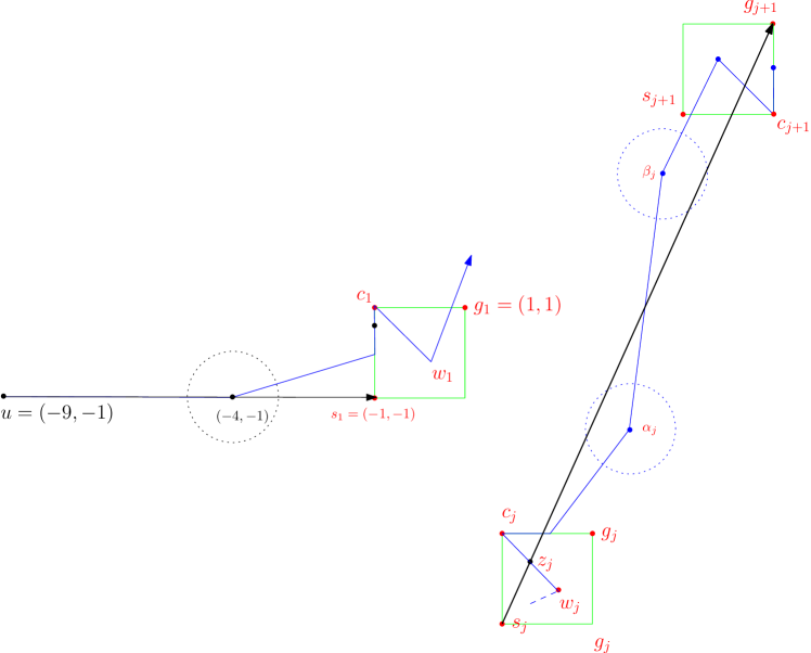
Figure 11: Proof of Lemma 2.7

if $x_{i}\in C_{1}$	location of ${\mathscr{O}}_{A}$	location of ${\mathscr{O}}_{L}$
	$u$	$u$
	$h_{1}$ s.t. $\|h_{1}\mu_{1}\|\leq\varepsilon$	$\mu_{1}=(-4,-1)$
	$s_{1}$	$M({\overline{s_{1}c_{1}}})$
if $\neg x_{i}\in C_{1}$	$u$	$u$
	$h_{1}$ s.t. $\|h_{1}\mu_{1}\|\leq\varepsilon$	$\mu_{1}=(-4,-1)$
	$s_{1}$	$\overrightarrow{\mu_{1}w_{1}}\dashv{\overline{s_{1}c_{1}}}$
if $x_{i}\notin C_{1}\&\neg x_{i}\notin C_{1}$	$u$	$u$
	$h_{1}$ s.t. $\|h_{1}\mu_{1}\|\leq\varepsilon$	$\mu_{1}=(-4,-1)$
	$s_{1}$	$\overrightarrow{\mu_{1}w_{1}}\dashv{\overline{s_{1}c_{1}}}$

Table 4: Proof of Lemma 2.3, the base case of induction

Proof of Lemma 3.2:

Proof .3.

We prove the lemma by induction on the number of edges in ${\mathscr{C}H}(S)$. Let $e_{1}e_{2}..e_{n}$ be the edges of ${\mathscr{P}}$, numbered after an arbitrary vertex of ${\mathscr{P}}$ in clockwise order. Obviously, to have a feasible curve, every point of $S$ must be located within some cylinder ${\mathscr{C}}(e_{i},\varepsilon)$. To establish the lemma, we show that when a feasible curve exists through $S$, the condition holds.

Imagine a point object ${\mathscr{O}}_{C}$ which cycles ${\mathscr{C}H}(S)$, starting from a vertex of ${\mathscr{C}H}(S)$, say point $u$, and ending at the same point. Let $u^{\prime}$ be a point on the boundary of ${\mathscr{P}}$ such that $\|uu^{\prime}\|\leq\varepsilon$. Imagine another point object ${\mathscr{O}}_{P}$ which starts from $u^{\prime}$, walks on the boundary of ${\mathscr{P}}$ until it reaches the same point $u^{\prime}$. Both of the objects walk clockwise.

To handle the base case of the induction, assume that the convex hull has an additional edge consist of only point $u$. Since the distance between ${\mathscr{O}}_{C}$ and ${\mathscr{O}}_{P}$ is less than $\varepsilon$ at the start, the base case of the induction holds. Assume inductively that ${\mathscr{O}}_{C}$ and ${\mathscr{O}}_{P}$ walk along their path, keeping distance $\varepsilon$ to each other, until ${\mathscr{O}}_{C}$ reaches to vertex $v$ in ${\mathscr{C}H}(S)$ and ${\mathscr{O}}_{P}$ reaches to point $v^{\prime}\in e_{i}$ on the boundary of ${\mathscr{P}}$ where $\|vv^{\prime}\|\leq\varepsilon$.

Let $w$ be the next vertex on ${\mathscr{C}H}(S)$ after $v$. If $w$ is located within the same cylinder ${\mathscr{C}}(e_{i},\varepsilon)$ as $v$, then by Observation 2, the lemma holds. Otherwise, assume that $w$ is in ${\mathscr{C}}(e_{j},\varepsilon)$, $i<j$ and $w^{\prime}$ is a point in $e_{j}$ where $\|ww^{\prime}\|\leq\varepsilon$. Consider the $\varepsilon$-ball around each of the vertices of the polygon between points $v^{\prime}$ and $w^{\prime}$. It suffices to show that edge $e=\overrightarrow{vw}$ crosses each of those balls.

Assume, for the sake of contradiction, that edge $e$ does not cross one of those balls, say the one around vertex $p$. Assume w.l.o.g. that all points in $S$ lie to the right of $e$. Then, two cases occur as illustrated in Figure 12: case (a), where ${\mathscr{B}}(p,e)$ lies to the right of $e$, which contradict the fact that the polygon is convex; or case (b), where ${\mathscr{B}}(p,e)$ lies to the left of $e$, which contradicts our assumption that a feasible curve exists, because no point in $S$ is in $\varepsilon$-distance to vertex $p$. ∎

t

Figure 12: Proof of Lemma 3.2

References

- [1] H. Alt and M. Godau. Computing the Fréchet distance between two polygonal curves. Int. J. of Comput. Geom. Appl., 5:75–91, 1995.
- [2] A. Maheshwari, J. Sack, K. Shahbaz, and H. Zarrabi-Zadeh. Staying close to a curve In Proc. 23rd Canadian Conference on Computational Geometry, pages 170–173, 2011.