Conditional hitting time estimation in a nonlinear filtering model by the Brownian bridge method

Abstract

The model consists of a signal process $X$ which is a general Brownian diffusion process and an observation process $Y$, also a diffusion process, which is supposed to be correlated to the signal process. We suppose that the process $Y$ is observed from time $0$ to $s>0$ at discrete times and aim to estimate, conditionally on these observations, the probability that the non-observed process $X$ crosses a fixed barrier after a given time $t>s$. We formulate this problem as a usual nonlinear filtering problem and use optimal quantization and Monte Carlo simulations techniques to estimate the involved quantities.

1 Introduction

We consider in this work a nonlinear filtering model where the signal process $X$ and the observation process $Y$ evolve following the stochastic differential equations:

$$\begin{cases}dX_{t}=b(X_{t},t)dt+\sigma(X_{t},t)dW_{t},&X_{0}=x_{0},\\ dY_{t}=h(Y_{t},X_{t},t)dt+\nu(Y_{t},t)dW_{t}+\delta(Y_{t},t)d\widetilde{W}_{t},&Y_{0}=y_{0}.\end{cases}$$ (1)

In these equations, $W$ and $\widetilde{W}$ are two independent standard real valued Brownian motions. We suppose that the functions $b$, $\sigma$, $h$, $\nu$, and $\delta$ are Lipschitz and that, for every $(x,t)\in]0,+\infty)^{2}$, $\delta(x,t)>0$, $\nu(x,t)>0$ and $\sigma(x,t)>0$.

Let ${\bf a}$ be a real number such that $0<{\bf a}<x_{0}$ and let

$$\tau_{\bf a}^{X}=\inf\{u\geq 0,X_{u}\leq{\bf a}\}$$

be the first hitting time of the barrier ${\bf a}$ by the signal process. As usually, we consider that $\inf\emptyset=+\infty$. Our aim is to estimate the distribution of the conditional hitting time

$$\mathds{P}\left(\tau_{\bf a}^{X}>t|\,\mathcal{F}_{s}^{Y}\right)$$ (2)

for $t\geq s>0$ and where $(\mathcal{F}_{t}^{Y})_{t\geq 0}$ is the filtration generated by the observation process $Y$:

$$\mathcal{F}_{s}^{Y}=\sigma(Y_{u},u\leq s).$$

More generally, we shall denote by $(\mathcal{F}_{t}^{Z})_{t\geq 0}$ the filtration generated by the process $Z$.

Such a problem arises for example in credit risk when modeling a credit event in a structural model as the first hitting time of a barrier ${\bf a}$ by the firm value process $X$. Investors are supposed to have no access to the true value of the firm but only to the observation process $Y$, which is correlated to the value of the firm (see e.g. [3, 4]). We will typically suppose that we observe the process $Y$ at regular discrete times $t_{0}=0<t_{1}<\ldots<t_{m}=s$ over the time interval $[0,s]$ and intend for estimating the quantity

$$\mathds{P}\left(\tau_{\bf a}^{X}>t|\,Y_{t_{0}},\ldots,Y_{t_{m}}\right)$$

for every $t\geq s$. Note that, if $t<s$, then, applying the Markov property to the diffusion $Y$, the computations boil down to the case $s=t$. In [2], the quantity

$$\mathds{P}\left(\inf_{u\in[s,t]}X_{u}>{\bf a}|Y_{t_{0}},\ldots,Y_{t_{m}}\right)$$

has been estimated by a hybrid Monte Carlo-Optimal quantization method in the case where the observation process dynamics is given by:

$$dY_{t}=Y_{t}\left(h(X_{t})dt+\nu(t)dW_{t}+\delta(t)d\widetilde{W}_{t}\right),\quad Y_{0}=y_{0},$$

where $\nu$ and $\delta$ are deterministic functions. However, the approach used in the previous work does not apply to our framework because we want to compute the conditional distribution of a function of the whole trajectory of the signal process from $0$ to $t$ given the observations from $0$ to $s$, with $s\leq t$.

Example 1.

A particular case of model (1) one may consider is the following “Black-Scholes” case:

$$\begin{cases}dX_{t}=X_{t}(\mu dt+\sigma dW_{t}),&X_{0}=x_{0},\\ dY_{t}=Y_{t}(rdt+\nu dW_{t}+\delta d\widetilde{W}_{t}),&Y_{0}=y_{0},\end{cases}$$ (3)

so that

$$\frac{dY_{t}}{Y_{t}}=\frac{\nu}{\sigma}\frac{dX_{t}}{X_{t}}+\big{(}r-\mu\frac{\nu}{\sigma}\big{)}dt+\delta d\widetilde{W}_{t},$$ (4)

or

$$Y_{t}=\frac{y_{0}}{(x_{0})^{\nu/\sigma}}X_{t}^{\nu/\sigma}\exp\left(\delta\widetilde{W}_{t}+\left(r-\frac{\nu^{2}+\delta^{2}}{2}-\frac{\mu\nu}{\sigma}+\frac{\nu\sigma}{2}\right)t\right).$$ (5)

Observe that setting $r=\mu$ and $\sigma=\nu$ yields

$$\frac{dY_{t}}{Y_{t}}=\frac{dX_{t}}{X_{t}}+\delta d\widetilde{W}_{t},$$

meaning that the return on $Y$ is the return on $X$ affected by a noise (see e.g. [3]).
Of course, in this case, we may compute theoretically the expression (2) by noticing that:

$$\tau_{\bf a}^{X} =\inf\{u\geq 0,X_{u}\leq{\bf a}\}$$

$$=\inf\left\{u\geq 0,\;\delta\widetilde{W}_{u}-\frac{\delta^{2}}{2}u\geq\ln(Y_{u})+\ln\left(\frac{x_{0}}{y_{0}}\right)-\ln(\bf a)\right\}$$

and that, conditionally to $\mathcal{F}_{s}^{Y}$, the process $\left(\widetilde{W}_{u},\;u\leq s\right)$ has the same law as

$$\left(\frac{\sigma}{\sqrt{\sigma^{2}+\delta^{2}}}B_{u}+\frac{\delta}{\sigma^{2}+\delta^{2}}\left(\ln(Y_{u})+\ln\left(\frac{x_{0}}{y_{0}}\right)+\frac{\sigma^{2}+\delta^{2}}{2}u\right),\;u\leq s\right)$$

where $B$ is a standard Brownian motion independent from the process $Y$. This follows from the fact that, since $W$ and $\widetilde{W}$ are two independent Brownian motion, so are

$$B=\frac{\sigma W+\delta\widetilde{W}}{\sqrt{\sigma^{2}+\delta^{2}}}\quad\text{ and }\quad\widetilde{B}=\frac{\delta W-\sigma\widetilde{W}}{\sqrt{\sigma^{2}+\delta^{2}}},$$

and from the relations :

$$B_{t}=\frac{1}{\sqrt{\sigma^{2}+\delta^{2}}}\left(\ln(Y_{t})+\ln\left(\frac{x_{0}}{y_{0}}\right)+\frac{\sigma^{2}+\delta^{2}}{2}t\right)\quad\text{ and }\quad\widetilde{W}_{t}=\frac{\delta B_{t}-\sigma\widetilde{B}_{t}}{\sqrt{\sigma^{2}+\delta^{2}}}.$$

Therefore, in this particular setting, the problem boils down to the computation of the first passage time of a Brownian motion to a curved boundary. We refer to [3] for some similar, and far more general, considerations.

Example 2.

Another particularly simple case is given when both the signal and the observation process evolve following the Ornstein-Uhlenbeck dynamics:

$$\begin{cases}dX_{t}=\lambda(\theta-X_{t})dt+\sigma dW_{t},&X_{0}=x_{0},\\ dY_{t}=\lambda(\theta-Y_{t})dt+\sigma dW_{t}+\delta d\widetilde{W}_{t},&Y_{0}=y_{0}.\end{cases}$$ (6)

In this case, we have :

$$X_{t}=Y_{t}-(y_{0}-x_{0})e^{-\lambda t}-\delta e^{-\lambda t}\int_{0}^{t}e^{\lambda u}d\widetilde{W}_{u},$$

so that

$$\tau_{\bf a}^{X}=\inf\left\{u\geq 0,\;Y_{u}-{\bf a}-(y_{0}-x_{0})e^{-\lambda u}\leq\delta e^{-\lambda u}\int_{0}^{u}e^{\lambda v}d\widetilde{W}_{v}\right\}$$

and, conditionally to $\mathcal{F}_{s}^{Y}$, the process $\displaystyle\left(e^{-\lambda u}\int_{0}^{u}e^{\lambda v}d\widetilde{W}_{v},\;u\leq s\right)$ has the same law as

$$\left(\frac{\sigma}{\sqrt{\sigma^{2}+\delta^{2}}}U_{u}+\frac{\delta e^{\lambda u}}{\sigma^{2}+\delta^{2}}\left(Y_{u}-y_{0}e^{-\lambda u}-\theta(1-e^{-\lambda u})\right),\;u\leq s\right)$$

where $U$ is an Ornstein-Uhlenbeck process with parameters $\lambda$ and 0 started from 0, and independent from $Y$. This follows from Knight’s representation theorem combined with the same ideas as above.

The rest of the paper is organized as follows: in Section 2, we state and prove the main theorems, i.e. we give an approximation of the expectation (2) when $X$ is replaced by its continuous Euler scheme $\bar{X}$, see especially Subsection 2.3. Then, in Section 3, we introduce some numerical tools in order to compute the quantities involved. We finally conclude the paper by a few simulations.

2 Estimation of the conditional survival probability

2.1 Preliminaries results

To deal with the computation of the conditional hitting time (2), we introduce the first hitting time from time $s$:

$$\tau^{(s)}=\inf\{u\geq s,X_{u}\leq{\bf a}\}.$$

Define furthermore the filtration $(\mathcal{G}_{t})_{t\geq 0}$ by, for every $t\geq 0$,

$$\mathcal{G}_{t}=\sigma\{(W_{u},\widetilde{W}_{u}),u\leq t\}.$$ (7)

We have the following result.

Lemma 2.1.

For every $t\geq s$,

$$\mathds{P}\big{(}\tau_{\bf a}^{X}>t|\,\mathcal{F}_{s}^{Y}\big{)} = \mathds{E}\Big{[}{1\!\!1}_{\{\tau_{\bf a}^{X}>s\}}F(s,t,X_{s})|\,\mathcal{F}_{s}^{Y}\Big{]}$$ (8)

with

$$F(s,t,X_{s})=\mathds{P}\left(\inf_{u\in[s,t]}X_{u}>{\bf a}|X_{s}\right).$$

Proof.

If $t\geq s$, one has

$$\{\tau_{\bf a}^{X}>t\}=\{\tau_{\bf a}^{X}>s\}\cap\{\tau^{(s)}>t\},$$

so that

$$\mathds{P}\big{(}\tau_{\bf a}^{X}>t|\,\mathcal{F}_{s}^{Y}\big{)} = \mathds{P}\big{(}\{\tau_{\bf a}^{X}>s\}\cap\{\tau^{(s)}>t\}|\,\mathcal{F}_{s}^{Y}\big{)}$$

$$= \mathds{E}\left[\mathds{E}\left[{1\!\!1}_{\{\tau_{\bf a}^{X}>s\}}{1\!\!1}_{\{\tau^{(s)}>t\}}|\mathcal{G}_{s}\right]|\mathcal{F}_{s}^{Y}\right],$$

where the $\sigma$-algebra $\mathcal{G}_{s}$ is defined in (7). Hence, using the fact that $\widetilde{W}$ is independent from $W$ and the Markov property of the process $X$:

$$\mathds{P}\big{(}\tau_{\bf a}^{X}>t|\,\mathcal{F}_{s}^{Y}\big{)} = \mathds{E}\left[{1\!\!1}_{\{\tau_{\bf a}^{X}>s\}}\mathds{E}\left[{1\!\!1}_{\{\tau^{(s)}>t\}}|\mathcal{G}_{s}\right]|\mathcal{F}_{s}^{Y}\right]$$

$$= \mathds{E}\left[{1\!\!1}_{\{\tau_{\bf a}^{X}>s\}}\mathds{E}\left[{1\!\!1}_{\{\tau^{(s)}>t\}}|\mathcal{F}_{s}^{W}\right]|\mathcal{F}_{s}^{Y}\right]$$

$$= \mathds{E}\left[{1\!\!1}_{\{\tau_{\bf a}^{X}>s\}}\mathds{P}\big{(}\tau^{(s)}>t|\mathcal{F}_{s}^{X}\big{)}|\mathcal{F}_{s}^{Y}\right]$$

$$= \mathds{E}\Big{[}{1\!\!1}_{\{\tau_{\bf a}^{X}>s\}}\mathds{P}\big{(}\inf_{u\in[s,t]}X_{u}>{\bf a}|X_{s}\big{)}|\mathcal{F}_{s}^{Y}\Big{]}.$$

This shows assertion (8). ∎

Note that in general, there is no closed-form expression for computing $\displaystyle\mathds{P}\big{(}\inf_{u\in[s,t]}X_{u}>{\bf a}|X_{s}\big{)}$, except in some very special cases, such as Brownian motion or Bessel processes… We shall therefore need an approximation of this expression, which is the purpose of the next subsection.

2.2 The continuous Euler scheme

Let us denote by $\bar{X}$ the continuous Euler scheme process associated to the signal process $X$ and defined by

$$\bar{X}_{s}=\bar{X}_{\underline{s}}+b(\bar{X}_{\underline{s}},\underline{s})(s-\underline{s})+\sigma(\bar{X}_{\underline{s}},\underline{s})(W_{s}-W_{\underline{s}}),\quad\bar{X}_{0}=x_{0},$$

with $\underline{s}=t_{k}$ if $s\in[t_{k},t_{k+1})$. To estimate the distribution of the conditional hitting time given in (2), consider that we observe the process $Y$ at discrete and regularly spaced times: $t_{0},t_{1},\dots,t_{m}$, with $0=t_{0}<\dots<t_{m}=s<t_{m+1}<\dots<t_{n}=t$. In our general model (see Equation (1)), the discrete time observation processes $\{\bar{X}_{t_{k}},\ k=0,\dots,n\}$ and $\{Y_{t_{k}},\ k=0,\dots,m\}$ are obtained from Euler scheme as:

$$\begin{cases}\bar{X}_{t_{k+1}}=\bar{X}_{t_{k}}+b(\bar{X}_{t_{k}},t_{k})\Delta_{k}+\sigma(\bar{X}_{t_{k}},t_{k})(W_{t_{k+1}}-W_{t_{k}})\\ Y_{t_{k+1}}=Y_{t_{k}}+h(Y_{t_{k}},\bar{X}_{t_{k}},t_{k})\Delta_{k}+\nu(Y_{t_{k}},t_{k})(W_{t_{k+1}}-W_{t_{k}})+\delta(Y_{t_{k}},t_{k})(\widetilde{W}_{t_{k+1}}-\widetilde{W}_{t_{k}})\end{cases}$$ (9)

where $k=0,\dots,m-1$ for the observation process, $k$ going till $n-1$ for the signal process and $\Delta_{k}=t_{k+1}-t_{k}$. Note that if $t>s$, the number of discretization steps over $[0,s]$ may differ from the number of discretization steps over $[s,t]$ so that we choose

$$\left\{\begin{array}[]{ll}t_{k}=\frac{ks}{m}&\textrm{ for }k=0,\dots,m\\ \\ t_{k}=s+\frac{k(t-s)}{n}&\textrm{ for }k=m+1,\dots,n.\end{array}\right.$$

Supposing that we have observed the trajectory $(Y_{t_{0}},\ldots,Y_{t_{m}})$ of the observation process $Y$ we aim to estimate

$$\mathds{P}(\tau_{\bf a}^{X}>t_{n}|\,Y_{t_{0}},\dots,Y_{t_{m}})$$

by

$$\mathds{P}\big{(}\tau_{\bf a}^{\bar{X}}>t_{n}|\,Y_{t_{0}},\dots,Y_{t_{m}}\big{)},$$ (10)

where

$$\tau_{\bf a}^{\bar{X}}=\inf\{u\geq 0,\bar{X}_{u}\leq{\bf a}\}.$$

To this end, we will use a useful result called the regular Brownian bridge method. This result recalled below allows us to compute the distribution of the minimum (or the maximum) of the continuous Euler scheme $\bar{X}$ of the process $X$ over the time interval $[0,t]$, given its values at discrete and regular time observation points $0=t_{0}<t_{1}<\dots<t_{n}=t$ (see, e.g. [6, 7]).

Lemma 2.2.

Let $(X_{t})_{t\geq 0}$ be a diffusion process with dynamics given by

$$X_{t}=x+\int_{0}^{t}b(X_{u},u)du+\int_{0}^{t}\sigma(X_{u},u)dW_{u}$$

and let $(\bar{X}_{t})_{t\geq 0}$ be its associated continuous Euler process. Then, the following equality in law holds:

$$\mathcal{L}\Big{(}\min_{u\in[0,t]}\bar{X}_{u}|\bar{X}_{t_{k}}=x_{k},k=0,\cdots,n\Big{)}=\mathcal{L}\Big{(}\min_{k=0,\cdots,n-1}\left(H_{\Delta_{k}\sigma^{2}(x_{k},t_{k})}^{x_{k},x_{k+1}}\right)^{-1}(\Lambda_{k})\Big{)},$$ (11)

where $(\Lambda_{k})_{k=0,\cdots,n-1}$ are $i.i.d.$ random variables uniformly distributed over the unit interval and $\left(H_{\Delta_{k}\sigma^{2}(x_{k},t_{k})}^{x_{k},x_{k+1}}\right)^{-1}$ is the inverse function of the conditional cumulative function $H_{\Delta_{k}\sigma^{2}(x_{k},t_{k})}^{x_{k},x_{k+1}}$, defined by

$$H_{\Delta_{k}\sigma^{2}(x_{k},t_{k})}^{x_{k},x_{k+1}}(u):=\left\{\begin{array}[]{ll}\exp\Big{(}-\frac{2}{\Delta_{k}\sigma^{2}(x_{k},t_{k})}(u-x_{k})(u-x_{k+1})\Big{)}&\textrm{if }u\leq\min(x_{k},x_{k+1})\\ 1&\textrm{otherwise.}\end{array}\right.$$ (12)

In the following, we shall replace the expression $\sigma(x_{k},t_{k})$ in the expression of $H$ by $\sigma_{k}$ and rather write: $H_{\Delta_{k}\sigma_{k}^{2}}^{x_{k},x_{k+1}}$.

Short proof.

Observe first that, conditionally to $\{\bar{X}_{t_{k}}=x_{k};\;k=0,\cdots,n\}$, the random variables $\displaystyle\left\{\min_{u\in[t_{k},t_{k+1}]}\bar{X}_{u};\;k=0,\ldots,n-1\right\}$ are mutually independent, thanks to the independent increments property of Brownian motion. Then, it suffices to notice that computing the law of $\displaystyle\min_{u\in[t_{k},t_{k+1}]}\bar{X}_{u}$ conditionally to $\{\bar{X}_{t_{k}}=x_{k},\bar{X}_{t_{k+1}}=x_{k+1}\}$ amounts to computing the law of the hitting times of the bridge of a Brownian motion with drift. This law is well-known to be independent from the drift (i.e. from the function $b$ here) and to be given by an expression such as (12). ∎

In the rest of the paper, the function $1-H_{\Delta_{k}\sigma_{k}^{2}}^{x_{k},x_{k+1}}({\bf a})$ will be often used. We shall denote it by $G_{\Delta_{k}\sigma_{k}^{2}}^{x_{k},x_{k+1}}({\bf a})$, so that

$$G_{\Delta_{k}\sigma_{k}^{2}}^{x_{k},x_{k+1}}({\bf a})=\left(1-\exp\left(-\frac{2(x_{k}-{\bf a})(x_{k+1}-{\bf a})}{\Delta_{k}\sigma^{2}(x_{k},t_{k})}\right)\right){1\!\!1}_{\{x_{k}\geq{\bf a};\;x_{k+1}\geq{\bf a}\}}.$$ (13)

Now, in our set-up, we shall apply the Brownian bridge method to obtain the following lemma, which is taken from [2]:

Lemma 2.3.

We have

$$\mathds{P}\left(\inf_{u\in[t_{m},t_{n}]}\bar{X}_{u}>{\bf a}\big{|}(\bar{X}_{t_{k}})_{k=0,\dots,m}\right)=\prod_{k=m}^{n-1}G_{\Delta_{k}\sigma_{k}^{2}}^{\bar{X}_{t_{k}},\bar{X}_{t_{k+1}}}({\bf a}).$$ (14)

Proof..

It follows from Lemma 2.2 that

$$\mathds{P}\left(\inf_{u\in[t_{m},t_{n}]}\bar{X}_{u}>a\big{|}(\bar{X}_{t_{k}})_{k=0,\dots,m}\right) = \mathbb{P}\left(\min_{k=m,\cdots,n-1}\left(H_{\Delta_{k}\sigma_{k}^{2}}^{\bar{X}_{t_{k}},\bar{X}_{t_{k+1}}}\right)^{-1}(\Lambda_{k})>{\bf a}\right).$$

Since the function $H_{\Delta_{k}\sigma_{k}^{2}}^{z_{k},z_{k+1}}(\cdot)$ is non-decreasing and the $\Lambda_{k}$’s are i.i.d. uniformly distributed random variables, this reduces to:

$$\mathbb{P}\left(\min_{u\in[t_{m},t_{n}]}\bar{X}_{u}>a\big{|}(\bar{X}_{t_{k}})_{k=0,\dots,m}\right) = \prod_{k=m}^{n-1}\mathbb{P}\left(\Lambda_{k}\geq H_{\Delta_{k}\sigma_{k}^{2}}^{\bar{X}_{t_{k}},\bar{X}_{t_{k+1}}}({\bf a})\right)$$

$$= \prod_{k=m}^{n-1}\left(1-H_{\Delta_{k}\sigma_{k}^{2}}^{\bar{X}_{t_{k}},\bar{X}_{t_{k+1}}}({\bf a})\right).$$

This completes the proof. ∎

2.3 Main theorem

We now state and prove the main theorems of this section. We first show that the conditional hitting time of the continuous Euler process $\bar{X}$ given the discrete path observations $Y_{t_{0}},\dots,Y_{t_{m}}$ may be written as an expectation of an explicit functional of the discrete path $\bar{X}_{t_{0}},\dots,\bar{X}_{t_{m}}$ of the signal given the observations $Y_{t_{0}},\dots,Y_{t_{m}}$. Therefore, we reduce the initial problem to the characterization of the conditional distribution of $\bar{X}_{t_{0}},\dots,\bar{X}_{t_{m}}$ given $Y_{t_{0}},\dots,Y_{t_{m}}$.

Theorem 2.4.

Set $\bar{X}^{m}=(\bar{X}_{t_{0}},\dots,\bar{X}_{t_{m}})$ and $Y^{m}=(Y_{t_{0}},\dots,Y_{t_{m}})$. We have:

$$\mathds{P}\big{(}\tau_{\bf a}^{\bar{X}}>t_{n}|\,Y_{t_{0}},\dots,Y_{t_{m}}\big{)}=\Psi(Y_{t_{0}},\dots,Y_{t_{m}}),$$ (15)

where for $y^{m}:=(y_{0},\dots,y_{m})$,

$$\Psi(y^{m})=\mathds{E}\big{[}\Phi\big{(}\bar{X}^{m}\big{)}\big{|}Y^{m}=y^{m}\big{]}.$$ (16)

The function $\Phi$ is defined for every $z^{m}=(z_{0},\dots,z_{m})$ by

$$\Phi(z^{m})=\bar{F}(t_{m},t_{n},z_{m})\prod_{k=0}^{m-1}G_{\Delta_{k}\sigma_{k}^{2}}^{z_{k},z_{k+1}}({\bf a}),$$

with

$$\bar{F}(t_{m},t_{n},x)=\mathds{E}\left[\prod_{k=m}^{n-1}G_{\Delta_{k}\sigma_{k}^{2}}^{\bar{X}_{t_{k}},\bar{X}_{t_{k+1}}}({\bf a})\big{|}\,\bar{X}_{t_{m}}=x\right].$$

Proof.

We may show similarly to Equation (8) in Lemma 2.1 that

$$\mathds{P}\big{(}\tau_{\bf a}^{\bar{X}}>t_{n}\big{|}\,Y_{t_{0}},\dots,Y_{t_{m}}\big{)}=\mathds{E}\left[{1\!\!1}_{\{\tau_{{\bf a}}^{\bar{X}}>t_{m}\}}\bar{F}(t_{m},t_{n},\bar{X}_{t_{m}})|\,Y_{t_{0}},\dots,Y_{t_{m}}\right],$$

with

$$\bar{F}(t_{m},t_{n},\bar{X}_{t_{m}})=\mathds{P}\left(\inf_{u\in[t_{m},t_{n}]}\bar{X}_{u}>{\bf a}\big{|}\bar{X}_{t_{m}}\right).$$

It follows from Lemma 2.3 that

$$\bar{F}(t_{m},t_{n},\bar{X}_{t_{m}})=\mathds{E}\left[\mathbb{P}\left(\min_{u\in[t_{m},t_{n}]}\bar{X}_{u}>{\bf a}\big{|}(\bar{X}_{t_{k}})_{k=0,\dots,m}\right)\big{|}\bar{X}_{t_{m}}\right]=\mathds{E}\left[\prod_{k=m}^{n-1}G_{\Delta_{k}\sigma_{k}^{2}}^{\bar{X}_{t_{k}},\bar{X}_{t_{k+1}}}({\bf a})\big{|}\,\bar{X}_{t_{m}}\right].$$

On the other hand, combining a successive conditioning rule with the independence between $W$ and $\widetilde{W}$ gives :

$$\mathds{P}\big{(}\tau_{\bf a}^{\bar{X}}>t_{n}|\,Y_{t_{0}},\dots,Y_{t_{m}}\big{)} = \mathds{E}\left[\mathds{E}\left[{1\!\!1}_{\{\tau_{\bf a}^{\bar{X}}>t_{m}\}}\bar{F}(t_{m},t_{n},\bar{X}_{t_{m}})|(W_{t_{k}},\widetilde{W}_{t_{k}})_{k=0,\dots,m}\right]|\,Y^{m}\right]$$

$$= \mathds{E}\left[\mathds{E}\left[{1\!\!1}_{\{\tau_{\bf a}^{\bar{X}}>t_{m}\}}\bar{F}(t_{n},t_{m},\bar{X}_{t_{m}})|(W_{t_{k}})_{k=0,\dots,m}\right]|\,Y^{m}\right]$$

$$= \mathds{E}\left[\bar{F}(t_{m},t_{n},\bar{X}_{t_{m}})\mathds{P}\left(\tau_{{\bf a}}^{\bar{X}}>t_{m}|(W_{t_{k}})_{k=0,\dots,m}\right)|\,Y^{m}\right]$$

$$= \mathds{E}\left[\bar{F}(t_{m},t_{n},\bar{X}_{t_{m}})\mathds{P}\left(\tau_{{\bf a}}^{\bar{X}}>t_{m}|(\bar{X}_{t_{k}})_{k=0,\dots,m}\right)|\,Y^{m}\right].$$

Now, using Lemma 2.3 once again, we have

$$\mathds{P}\left(\tau_{{\bf a}}^{\bar{X}}>t_{m}|(\bar{X}_{t_{k}})_{k=0,\dots,m}\right)=\prod_{k=0}^{m-1}G_{\Delta_{k}\sigma_{k}^{2}}^{\bar{X}_{t_{k}},\bar{X}_{t_{k+1}}}({\bf a})$$

so that

$$\mathds{P}\big{(}\tau_{\bf a}^{\bar{X}}>t_{n}|\,Y_{t_{0}},\dots,Y_{t_{m}}\big{)}=\mathds{E}\left[\Phi(\bar{X}^{m})\,|\,Y_{t_{0}},\dots,Y_{t_{m}}\right]$$

where for every $x^{m}:=(x_{0},\dots,x_{m})$,

$$\Phi(x^{m})=\bar{F}(t_{m},t_{n},x_{m})\prod_{k=0}^{m-1}G_{\Delta_{k}\sigma_{k}^{2}}^{x_{k},x_{k+1}}({\bf a}).$$

This completes the proof. ∎

It remains now to characterize the law of $\bar{X}^{m}|Y^{m}=y^{m}$ appearing in (16). This is the purpose of the following theorem, in which we shall write the conditional survival probability in a usual form with respect to standard nonlinear filtering problems.
We set from now on $\sigma_{k}=\sigma(x_{k},t_{k}),b_{k}=b(x_{k},t_{k}),\delta_{k}=\delta(y_{k},t_{k}),h_{k}=h(y_{k},x_{k},t_{k})$, and $\nu_{k}=\nu(y_{k},t_{k})$. We next give the main result of the paper.

Theorem 2.5.

We have:

$$\mathds{P}\big{(}\tau_{\bf a}^{\bar{X}}>t_{n}|\,Y_{t_{0}},\dots,Y_{t_{m}}\big{)}=\Psi(Y_{t_{0}},\dots,Y_{t_{m}}),$$ (17)

where for $y^{m}:=(y_{0},\dots,y_{m})$,

$$\Psi(y^{m})=\frac{\mathds{E}\big{[}\bar{F}(t_{m},t_{n},\bar{X}_{t_{m}})K^{m}L_{y}^{m}\big{]}}{\mathds{E}[L_{y}^{m}]},$$ (18)

with

$$K^{m}=\prod_{k=0}^{m-1}G_{\Delta_{k}\sigma_{k}^{2}}^{\bar{X}_{t_{k}},\bar{X}_{t_{k+1}}}({\bf a})\quad\textrm{and}\quad L_{y}^{m}=\prod_{k=0}^{m-1}g_{k}(\bar{X}_{t_{k}},y_{k};\bar{X}_{t_{k+1}},y_{k+1}).$$

The function $g_{k}$ is defined by

$$g_{k}(x_{k},y_{k};x_{k+1},y_{k+1})=\frac{1}{(2\pi\Delta_{k})^{3/2}\sigma^{2}_{k}\delta_{k}}\exp\Bigg{(}-\frac{\nu_{k}^{2}}{2\delta^{2}_{k}\Delta_{k}}\Big{(}\frac{x_{k+1}-m_{k}^{1}}{\sigma_{k}}-\frac{y_{k+1}-m_{k}^{2}}{\nu_{k}}\Big{)}^{2}\Bigg{)}$$ (19)

with $m_{k}^{1}:=x_{k}+b_{k}\Delta_{k}\;$ and $\;m_{k}^{2}:=y_{k}+h_{k}\Delta_{k}$.

Proof.

It follows from Theorem 2.4 that

$$\mathds{P}\big{(}\tau_{\bf a}^{\bar{X}}>t_{n}|\,Y_{t_{0}},\dots,Y_{t_{m}}\big{)}=\mathds{E}\left[\Phi(\bar{X}^{m})\,|\,Y_{t_{0}},\dots,Y_{t_{m}}\right]$$

where for every $x^{m}:=(x_{0},\dots,x_{m})$,

$$\Phi(x^{m})=\bar{F}(t_{m},t_{n},x_{m})\prod_{k=0}^{m-1}G_{\Delta_{k}\sigma_{k}^{2}}^{x_{k},x_{k+1}}({\bf a}).$$

It remains to characterize the conditional distribution of $\bar{X}^{m}$ given $Y^{m}$. Recall that the dynamics of the processes $(\bar{X}_{t_{k}})$ and $(Y_{t_{k}})$ are given for $k=0,\dots,m$ by

$$\begin{cases}\displaystyle\bar{X}_{t_{k+1}}=\bar{X}_{t_{k}}+b(\bar{X}_{t_{k}},t_{k})\Delta_{k}+\sigma(\bar{X}_{t_{k}},t_{k})(W_{t_{k+1}}-W_{t_{k}})\\ \displaystyle Y_{t_{k+1}}=Y_{t_{k}}+h(Y_{t_{k}},\bar{X}_{t_{k}},t_{k})\Delta_{k}+\nu(Y_{t_{k}},t_{k})(W_{t_{k+1}}-W_{t_{k}})+\delta(Y_{t_{k}},t_{k})(\widetilde{W}_{t_{k+1}}-\widetilde{W}_{t_{k}})\end{cases}$$ (20)

Let $\mathds{P}_{x_{k},y_{k}}(\bar{X}_{t_{k+1}}\in dx_{k+1},Y_{t_{k+1}}\in dy_{k+1})$ denote the density function of the couple $(\bar{X}_{t_{k+1}},Y_{t_{k+1}})$ given $(\bar{X}_{t_{k}},Y_{t_{k}})=(x_{k},y_{k})$. Using Bayes formula and the Markov property of the process $(\bar{X}_{t_{k}},Y_{t_{k}})_{k}$ we get:

$$\mathds{P}_{x_{0},y_{0}}(\bar{X}_{t_{1}}\in dx_{1},\dots,\bar{X}_{t_{m}}\in dx_{m}|Y_{t_{1}}\in dy_{1},\dots,Y_{t_{m}}\in dy_{m})$$

$$\qquad\quad=\frac{\mathds{P}_{x_{0},y_{0}}\big{(}(\bar{X}_{t_{1}}\in dx_{1},Y_{t_{1}}\in dy_{1});\dots;(\bar{X}_{t_{m}}\in dx_{m},Y_{t_{m}}\in dy_{m})\big{)}}{\mathds{P}_{x_{0},y_{0}}(Y_{t_{1}}\in dy_{1},\dots,Y_{t_{m}}\in dy_{m})}$$

$$\qquad\quad=\frac{\mathds{P}_{x_{0},y_{0}}\big{(}\bar{X}_{t_{1}}\in dx_{1},Y_{t_{1}}\in dy_{1})\times\dots\times\mathds{P}_{x_{m-1},y_{m-1}}(\bar{X}_{t_{m}}\in dx_{m},Y_{t_{m}}\in dy_{m})}{\mathds{P}_{x_{0},y_{0}}(Y_{t_{1}}\in dy_{1},\dots,Y_{t_{m}}\in dy_{m})}.$$

For every $x^{m}=(x_{0},\dots,x_{m})$ and $y^{m}=(y_{0},\dots,y_{m})$, set :

$$N_{k}(x^{m};y^{m}):=\mathds{P}_{x_{0},y_{0}}\big{(}\bar{X}_{t_{1}}\in dx_{1},Y_{t_{1}}\in dy_{1})\times\dots\times\mathds{P}_{x_{m-1},y_{m-1}}(\bar{X}_{t_{m}}\in dx_{m},Y_{t_{m}}\in dy_{m}).$$

With this notation, the denominator reads:

$$\mathds{P}_{x_{0},y_{0}}(Y_{t_{1}}\in dy_{1},\dots,Y_{t_{m}}\in dy_{m})=\int N_{k}(x^{m};y^{m})dx_{1}\ldots dx_{m}.$$

On the other hand, the random vector $(\bar{X}_{t_{k+1}},Y_{t_{k+1}})\big{|}(\bar{X}_{t_{k}},Y_{t_{k}})=(x_{k},y_{k})$ has a Gaussian distribution with mean $m_{k}$ and covariance matrix $\Sigma_{k}$ given for every $k=0,\dots,m-1$ by

$$m_{k}=\begin{pmatrix}x_{k}+b_{k}\Delta_{k}\\ y_{k}+h_{k}\Delta_{k}\\ \end{pmatrix},\qquad\ \Sigma_{k}=\Delta_{k}\begin{pmatrix}\sigma^{2}_{k}&\sigma_{k}\nu_{k}\\ \sigma_{k}\nu_{k}&\quad\nu^{2}_{k}+\delta^{2}_{k}\end{pmatrix}.$$ (21)

Then, for every $k=0,\dots,m-1$, the density $f_{k}(x_{k},y_{k};x_{k+1},y_{k+1})$ of $(\bar{X}_{t_{k+1}},Y_{t_{k+1}})\big{|}(\bar{X}_{t_{k}},Y_{t_{k}})=(x_{k},y_{k})$ reads

$$f_{k}(x_{k},y_{k};x_{k+1},y_{k+1})=\frac{1}{2\pi\sigma_{k}\delta_{k}\Delta_{k}}\exp\Bigg{(} -\frac{\nu^{2}_{k}+\delta^{2}_{k}}{2\delta^{2}_{k}\Delta_{k}}\Big{\{}\frac{(x_{k+1}-m_{k}^{1})^{2}}{\sigma^{2}_{k}}+\frac{(y_{k+1}-m_{k}^{2})^{2}}{\nu^{2}_{k}+\delta^{2}_{k}}$$

$$-\frac{2\nu_{k}}{\sigma_{k}(\nu^{2}_{k}+\delta^{2}_{k})}(x_{k+1}-m_{k}^{1})(y_{k+1}-m_{k}^{2})\Big{\}}\Bigg{)},$$ (22)

where $m_{k}^{1}:=x_{k}+b_{k}\Delta_{k}\;$ and $\;m_{k}^{2}:=y_{k}+h_{k}\Delta_{k}$. As a consequence,

$$\mathds{P}\left(\tau_{\bf a}^{\bar{X}}>t_{n}|\,(Y_{t_{0}},\dots,Y_{t_{m}})=y^{m}\right) = \mathds{E}\left[\Phi(\bar{X}^{m})\,|\,(Y_{t_{0}},\dots,Y_{t_{m}})=y^{m}\right]$$ (23)

$$= \frac{\int\Phi(x^{m})N_{k}(x^{m};y^{m})dx_{1}\ldots dx_{m}}{\int N_{k}(x^{m};y^{m})dx_{1}\ldots dx_{m}}.$$

Now, we know that the random variable $\bar{X}_{t_{k+1}}|\bar{X}_{t_{k}}=x_{k}$ has a Gaussian distribution with mean $m_{k}^{1}$ and variance $\sigma^{2}_{k}\Delta_{k}$. Its density $P_{k}(x_{k},x_{k+1})dx_{k+1}$ is therefore given by :

$$P_{k}(x_{k},x_{k+1})dx_{k+1}=\frac{1}{\sqrt{2\pi\Delta_{k}}\,\sigma_{k}}\exp\Big{(}-\frac{(x_{k+1}-m_{k}^{1})^{2}}{2\sigma^{2}_{k}\Delta_{k}}\Big{)}dx_{k+1}.$$

Then, by definition of $N_{k}$, we may write:

$$\int N_{k}(x^{m};y^{m})dx_{1}\ldots dx_{m}$$

$$= \int\prod_{k=0}^{m-1}f_{k}(x_{k},y_{k};x_{k+1},y_{k+1})dx_{k+1}$$

$$= \int\prod_{k=0}^{m-1}\frac{f_{k}(x_{k},y_{k};x_{k+1},y_{k+1})}{P_{k}(x_{k},x_{k+1})}P_{k}(x_{k},x_{k+1})dx_{k+1}$$

$$= \int\left(\prod_{k=0}^{m-1}\frac{f_{k}(x_{k},y_{k};x_{k+1},y_{k+1})}{P_{k}(x_{k},x_{k+1})}\right)\prod_{k=0}^{m-1}P_{k}(x_{k},x_{k+1})dx_{k+1}$$

$$= \int\left(\prod_{k=0}^{m-1}g_{k}(x_{k},y_{k};x_{k+1},y_{k+1})\right)\mathds{P}_{x_{0},y_{0}}(\bar{X}_{t_{1}}\in dx_{1},\dots,\bar{X}_{t_{m}}\in dx_{m})=\mathds{E}[L_{y}^{m}],$$

where $g_{k}$ is defined by (19) and the next-to-last equality follows from the Markov property of the process $(\bar{X}_{t_{k}},\;k=0,\ldots,m)$. Now, looking at the numerator of (23), similar computations lead to:

$$\int\Phi(x^{m})N_{k}(x^{m};y^{m})dx_{1}\ldots dx_{m}$$

$$= \int\bar{F}(t_{m},t_{n},x_{m})\prod_{k=0}^{m-1}G_{\Delta_{k}\sigma_{k}^{2}}^{x_{k},x_{k+1}}({\bf a})f_{k}(x_{k},y_{k};x_{k+1},y_{k+1})dx_{k+1},$$

$$= \int\bar{F}(t_{m},t_{n},x_{m})\left(\prod_{k=0}^{m-1}G_{\Delta_{k}\sigma_{k}^{2}}^{x_{k},x_{k+1}}({\bf a})\right)$$

$$\qquad\qquad\times\left(\prod_{k=0}^{m-1}g_{k}(x_{k},y_{k};x_{k+1},y_{k+1})\right)\mathds{P}_{x_{0},y_{0}}(\bar{X}_{t_{1}}\in dx_{1},\dots,\bar{X}_{t_{m}}\in dx_{m})$$

$$= \mathds{E}\big{[}\bar{F}(t_{m},t_{n},\bar{X}_{t_{m}})K^{m}L_{y}^{m}\big{]}.$$

Finally, going back to (23), we obtain

$$\mathds{P}\left(\tau_{\bf a}^{\bar{X}}>t_{n}|\,(Y_{t_{0}},\dots,Y_{t_{m}})=y^{m}\right)=\frac{\mathds{E}\big{[}\bar{F}(t_{m},t_{n},\bar{X}_{t_{m}})K^{m}L_{y}^{m}\big{]}}{\mathds{E}[L_{y}^{m}]}$$

which is the announced result. ∎

Remark 2.1.

Remark that more generally we have for every real valued bounded function $f$,

$$\mathds{E}[f(\bar{X}_{t_{m}})|Y_{t_{0}}=y_{0},\dots,Y_{t_{m}}=y_{m}]=\frac{\mathds{E}\big{[}f(\bar{X}_{t_{m}})L_{y}^{m}\big{]}}{\mathds{E}[L_{y}^{m}]}.$$ (24)

In this case we can estimate the right hand side quantity of (24) using recursive algorithms. In our setting, we can adapt these algorithms by noting that the expression (18) may be read in the similar form of (24) as:

$$\mathds{P}\left(\tau_{\bf a}^{\bar{X}}>t_{n}|\,(Y_{t_{0}},\dots,Y_{t_{m}})=y^{m}\right)=\frac{\mathds{E}\big{[}\bar{F}(t_{m},t_{n},\bar{X}_{t_{m}})L_{y}^{{}^{\prime}m}\big{]}}{\mathds{E}[L_{y}^{m}]}$$

where

$$L_{y}^{{}^{\prime}m}=\prod_{k=0}^{m-1}g_{k}(\bar{X}_{t_{k}},y_{k};\bar{X}_{t_{k+1}},y_{k+1})G_{\Delta_{k}\sigma_{k}^{2}}^{\bar{X}_{t_{k}},\bar{X}_{t_{k+1}}}({\bf a})$$

and where the involved functions are defined in Theorem 2.5.

Considering the model given in Example 1, one may apply the result of Theorem 2.5 using the continuous Euler process $\bar{X}$ of the signal. However since in this framework the solutions of the stochastic differential equations are explicit, we refrain from using the Euler scheme to avoid adding additional error. In the next result we deduce a similar representation of the conditional survival probability using the explicit solutions of the stochastic differential equations of the model (3).

Corollary 2.6.

Consider that the signal process $X$ and the observation process $Y$ evolve following the stochastic differential equations given in (3):

$$\begin{cases}dX_{t}=X_{t}(\mu dt+\sigma dW_{t}),&X_{0}=x_{0},\\ dY_{t}=Y_{t}(rdt+\nu dW_{t}+\delta d\widetilde{W}_{t}),&Y_{0}=y_{0}.\end{cases}$$ (25)

Then,

$$\Psi(y^{m})=\frac{\mathds{E}\big{[}F(t_{m},t_{n},X_{t_{m}})K^{m}L_{y}^{m}\big{]}}{\mathds{E}[L_{y}^{m}]},$$ (26)

with

$$K^{m}=\prod_{k=0}^{m-1}G_{\Delta_{k}\sigma_{k}^{2}}^{X_{t_{k}},X_{t_{k+1}}}({\bf a})\quad\textrm{and}\quad L_{y}^{m}=\prod_{k=0}^{m-1}g_{k}(X_{t_{k}},y_{k};X_{t_{k+1}},y_{k+1}).$$

The function $g_{k}$ is defined by

$$g_{k}(x_{k},y_{k};x_{k+1},y_{k+1})=\frac{1}{(2\pi\Delta_{k})^{3/2}\pi_{k}}\exp\Bigg{(}-\frac{\nu^{2}}{2\delta^{2}\Delta_{k}}\Big{(}\frac{\log x_{k+1}-m_{k}^{1}}{\sigma}-\frac{\log y_{k+1}-m_{k}^{2}}{\nu}\Big{)}^{2}\Bigg{)}$$ (27)

with

$$\pi_{k}:=\sigma^{2}\delta x_{k+1}^{2}y_{k+1},\quad m_{k}^{1}:=\log x_{k}+(\mu-\frac{1}{2}\sigma^{2})\Delta_{k}\quad\text{and}\quad m_{k}^{2}:=\log y_{k}+(r-\frac{1}{2}\nu^{2}-\frac{1}{2}\delta^{2})\Delta_{k}.$$

Proof..

It follows from Itô formula that for every $s\leq t$,

$$\begin{cases}X_{t}=X_{s}\exp\left((\mu-\frac{1}{2}\sigma^{2})(t-s)+\sigma(W_{t}-W_{s})\right)\\ Y_{t}=Y_{s}\exp\left((r-\frac{1}{2}\nu^{2}-\frac{1}{2}\delta^{2})(t-s)+\nu(W_{t}-W_{s})+\delta(\widetilde{W}_{t}-\widetilde{W}_{s})\right).\end{cases}$$ (28)

Then, for every $k=0,\dots,m-1$ the random vector $(X_{t_{k+1}},Y_{t_{k+1}})|(X_{t_{k}},Y_{t_{k}})=(x_{k},y_{k})$ has a bivariate lognormal distribution with mean $m_{k}$ and covariance matrix $\Sigma$ given by

$$m_{k}=\begin{pmatrix}\log x_{k}+(\mu-\frac{1}{2}\sigma^{2})\Delta_{k}\\ \log y_{k}+(r-\frac{1}{2}\nu^{2}-\frac{1}{2}\delta^{2})\Delta_{k}\\ \end{pmatrix},\qquad\ \Sigma=\Delta_{k}\begin{pmatrix}\sigma^{2}&\sigma\nu\\ \sigma\nu&\quad\nu^{2}+\delta^{2}\end{pmatrix}.$$

Hence, its density reads (setting $\mu_{k}=\sigma\delta x_{k+1}y_{k+1}$)

$$f_{k}(x_{k},y_{k};x_{k+1},y_{k+1})=\frac{1}{2\pi\Delta_{k}\mu_{k}}\exp\Bigg{(} - \frac{\nu^{2}+\delta^{2}}{2\delta^{2}\Delta_{k}}\Big{\{}\frac{(\log x_{k+1}-m_{k}^{1})^{2}}{\sigma^{2}}$$

$$- \frac{2\nu}{\sigma(\nu^{2}+\delta^{2})}(\log x_{k+1}-m_{k}^{1})(\log y_{k+1}-m_{k}^{2})$$

$$+ \frac{(\log y_{k+1}-m_{k}^{2})^{2}}{\nu^{2}+\delta^{2}}\Big{\}}\Bigg{)},$$

where $m_{k}^{1}=\log x_{k}+(\mu-\frac{1}{2}\sigma^{2})\Delta_{k}$ and $m_{k}^{2}:=\log y_{k}+(r-\frac{1}{2}\nu^{2}-\frac{1}{2}\delta^{2})\Delta_{k}$. Furthermore, for every $k=0,\dots,m-1$, the random variable $X_{t_{k+1}}|X_{t_{k}}=x_{k}$ has a lognormal distribution with mean $m_{k}^{1}$ and variance $\sigma^{2}$ so that its density distribution $P_{k}(x_{k},x_{k+1})$ is given by

$$P_{k}(x_{k},x_{k+1})=\frac{1}{\sqrt{2\pi\Delta_{k}}\,\sigma x_{k+1}}\exp\Big{(}-\frac{(\log x_{k+1}-m_{k}^{1})^{2}}{2\sigma^{2}\Delta_{k}}\Big{)}.$$

We then conclude the proof by using the same arguments than those of the proof of Theorem 2.5. ∎

There exist several methods to estimate the above representation of the conditional survival probability. These methods involve, amount others, Monte Carlo simulations and optimal quantization methods. Owing to the numerical performance of the optimal quantization method due for example to its fast performability as soon as the optimal grids are obtained, we will use optimal quantization methods to estimate the conditional survival probability.

The use of optimal quantization methods to estimate the filter supposes to have numerical access to optimal (or stationary) quantizers of the marginals of the signal process. One may use the optimal vector quantization method (as done in the seminal work [11] and used in [2]) to estimate these marginals. This method requires the use of some algorithms, like stochastic algorithms or Lloyd’s algorithm, to obtain numerically the optimal (or stationary) quantizers of the marginals of the signal process. Given these optimal quantizers, the filter estimation is obtained quite instantaneously. However, the step of search of stationary quantizers is very time consuming.

We propose here an alternative method, the (quadratic) marginal functional quantization method (introduce in [14] to price barrier options), to quantize the marginals of the signal process. The marginal functional quantization method consists first in considering the ordinary differential equation (ODE) resulting to the substitution of the Brownian motion appearing in the dynamics of the signal process by a quadratic quantization of the Brownian motion. Then, by constructing some “good” marginal quantization of the signal process based on the solution of the previous ODE’s, we will show how to estimate the nonlinear filter. Since this procedure is based on the quantization of the Brownian motion and skips the use of algorithms to perform the stationary quantizers, the computation of the marginal quantizers is quite instantaneous. This reduce drastically the time computation of the procedure with respect to the vector quantization method since we skip the step of the use of algorithms search of marginal quantizers by using instead, the marginals of the functional quantization of the signal process.

In the rest of the paper we deal with the estimations methods of the conditional survival probability.

3 Numerical tools

Our aim in this section is to derive a way to compute numerically the conditional survival probability using Equation (18). To this end, we have to estimate three quantities: the quantity $\bar{F}(t_{m},t_{n},\bar{X}_{t_{m}})$, the expectation $\mathds{E}[\bar{F}(t_{m},t_{n},\bar{X}_{t_{m}})K^{m}L_{y}^{m}]$ as soon as $\bar{F}(t_{m},t_{n},\bar{X}_{t_{m}})$ is estimated, and finally, the expectation $\mathds{E}[L_{y}^{m}]$. Both expectations will be estimated using marginal functional quantization method. The probability $\bar{F}(t_{m},t_{n},\bar{X}_{t_{m}})$ will be estimated by Monte Carlo simulations.

Before dealing with the estimation tools, we shall recall first some basic results about both optimal vector quantization and functional quantization. Then, we will show how to construct the marginal functional quantization process which will be used to estimate the quantities of interest.

3.1 Overview on optimal quantization methods

The optimal vector quantization on a grid $\Gamma=\{x_{1},\cdots,x_{N}\}$ (which will be called a quantizer) of an $\mathbb{R}^{d}$-valued random vector $X$ defined on a probability space $(\Omega,\mathcal{A},\mathbb{P})$ with finite $r$-th moment and probability distribution $\mathbb{P}_{X}$ consists in finding the best approximation of $X$ by a Borel function of $X$ taking at most $N$ values. This turns out to find the solution of the following minimization problem:

$$e_{N,r}(X)=\inf{\{\|X-\widehat{X}^{\Gamma}\|_{r},\Gamma\subset\mathbb{R}^{d},|\Gamma|\leq N\}},$$ (29)

where ${\|X\|}_{r}:={\left(\mathbb{E}[{|X|}^{r}]\right)}^{1/r}$ and where $\widehat{X}^{\Gamma}:=\sum_{i=1}^{N}x_{i}{1\!\!1}_{\{X\in C_{i}(\Gamma)\}}$ is the quantization of $X$ (we will write $\widehat{X}^{N}$ instead of $\widehat{X}^{\Gamma}$) on the grid $\Gamma$ and $(C_{i}(\Gamma))_{i=1,\dots,N}$ corresponds to a Voronoi tessellation of $\mathbb{R}^{d}$ (with respect to a norm $|\cdot|$ on $\mathbb{R}^{d}$), that is, a Borel partition of $\mathbb{R}^{d}$ satisfying for every $i$,

$$C_{i}(\Gamma)\subset\{x\in\mathbb{R}^{d}:|x-x_{i}|=\min_{j=1,\dots,N}|x-x_{j}|\}.$$

We know that for every $N\geq 1$, the infimum in $(\ref{EqDefErrorQuant})$ is reached at one grid $\Gamma^{\star}$ at least, called a $L^{r}$-optimal $N$-quantizer. It is also known that if $\textrm{ card(supp}(\mathbb{P}_{X}))\geq N$ then $|\Gamma|=N$ (see e.g. [8] or [10]). Moreover, the $L^{r}$-mean quantization error $e_{N,r}(X)$ decreases to zero at an $N^{-1/d}$-rate as the size $N$ of the grid $\Gamma$ goes to infinity. This convergence rate has been investigated in [1] and [15] for absolutely continuous probability measures under the quadratic norm on $\mathbb{R}^{d}$, and studied in great details in [8] under an arbitrary norm on $\mathbb{R}^{d}$ for absolutely continuous measures and some singular measures.

From the numerical integration viewpoint, finding an optimal quantization grid $\Gamma^{\star}$ may be a challenging task. In practice (we will only consider the quadratic case, i.e. when $r=2$) we are sometimes led to find some “good” quantizations ${\rm Proj}_{\Gamma}(X)$ (with $\Gamma=\{x_{1},\dots,x_{N}\}$) which are close to $X$ in distribution, so that for every Borel function $F:\mathbb{R}^{d}\mapsto\mathbb{R}$, we can approximate $\mathbb{E}[F(X)]$ by

$$\mathbb{E}\left[F\big{(}\widehat{X}^{N}\big{)}\right]=\sum_{i=1}^{N}F(x_{i})\ p_{i},$$ (30)

where $p_{i}=\mathbb{P}\big{(}{\rm Proj}_{\Gamma}(X)=x_{i}\big{)}.$ Amount “good” quantizations of $X$ we have stationary quantizers. A grid $\Gamma$ inducing the quantization $\widehat{X}^{N}$ of $X$ is said stationary if

$$\forall\ i\neq j,\quad\ \ x_{i}\neq x_{j}\ \ \mbox{and}\ \ \mathbb{P}\left(X\in\cup_{i}\partial C_{i}(\Gamma)\right)=0$$ (31)

and

$$\mathbb{E}\left[X|\widehat{X}^{N}\right]=\widehat{X}^{N}.$$

The stationary quantizers search is based on zero search recursive procedures like Newton algorithm in the one dimensional framework and some algorithms as Lloyd’s I algorithms (see e.g. [5]), the Competitive Learning Vector Quantization (CLVQ) algorithm (see [5]) or stochastic algorithms (see [12]) in the multidimensional framework. Note that optimal quantizers estimates of the multivariate Gaussian random vector are available in the website www.quantize.math-fi.com.

We next recall some error bounds induced from approximating $\mathbb{E}[F(X)]$ by (30). Let $\Gamma$ be a stationary quantizer and $F$ be a Borel function on $\mathbb{R}^{d}$.

• If $F$ is convex then

  $$\mathbb{E}\big{[}F(\widehat{X}^{N})\big{]}\leq\mathbb{E}[F(X)].$$

• Lipschitz functions:

  • If $F$ is Lipschitz continuous then (this error bound doesn’t require the quantizer $\Gamma$ to be stationary)

    $$\big{|}\mathbb{E}[F(X)]-\mathbb{E}[F(\widehat{X}^{N})]\big{|}\leq[F]_{Lip}\|X-\widehat{X}^{N}\|_{2},$$

    where

    $$[F]_{{\rm Lip}}:=\sup_{x\not=y}\frac{|F(x)-F(y)|}{|x-y|}.$$

  • Let $\theta:\mathbb{R}^{d}\rightarrow\mathbb{R}_{+}$ be a nonnegative convex function such that $\theta(X)\in L^{2}(\mathbb{P})$. If $F$ is locally Lipschitz with at most $\theta$-growth, i.e. $\left|F(x)-F(y)\right|\leq[F]_{Lip}|x-y|\left(\theta(x)+\theta(y)\right)$ then $F(X)\in L^{1}(\mathbb{P})$ and

    $$\big{|}\mathbb{E}[F(X)]-\mathbb{E}[F(\widehat{X}^{N})]\big{|}\leq 2[F]_{Lip}\|X-\widehat{X}^{N}\|_{2}\|\theta(X)\|_{2}.$$

• Differentiable functionals:
  If $F$ is differentiable on $\mathbb{R}^{d}$ with an $\alpha$-Hölder differential D$F$ ($\alpha\in[0,1]$), then

  $$\big{|}\mathbb{E}[F(X)]-\mathbb{E}[F(\widehat{X}^{N})]\big{|}\leq[DF]_{\alpha}\|X-\widehat{X}^{N}\|_{2}^{1+\alpha}.$$

Other error bounds related to the regularity of $F$ may be found in [13]).

The optimal vector quantization may be extended to random vectors with values in a set of infinite dimension, in particular to stochastic processes viewed as random variables with values in $L^{2}([0,T],dt)$ endowed with the norm

$$\mathbb{E}\left[|X|_{L^{2}_{T}}^{2}\right]=\int_{0}^{T}\mathbb{E}[X^{2}_{s}]ds<+\infty.$$

The functional quantization of the stochastic process $(X_{t})_{t\in[0,T]}$ with dynamics

$$dX_{t}=b(X_{t},t)dt+\sigma(X_{t},t)dW_{t},\quad X_{0}=x\in\mathbb{R},$$

is based on the functional quantization of the Brownian motion $W$. One way to quantize the Brownian motion is to use the optimal product quantization using its Karhunen-Loève expansion which reads :

$$W\;\stackrel{{\scriptstyle L^{2}_{T}}}{{=}}\;\sum_{n\geq 1}\sqrt{\lambda_{n}}\xi_{n}e_{n},$$

where $\xi_{n}:=\left\langle W,e_{n}\right\rangle/\sqrt{\lambda_{n}}$, $n\geq 1$, is a sequence of i.i.d. random variables with standard normal distribution and

$$e_{n}(t)=\sqrt{\frac{2}{T}}\sin\left(\pi\left(n-\frac{1}{2}\right)\frac{t}{T}\right),\ \ \lambda_{n}=\left(\frac{T}{\pi\left(n-\frac{1}{2}\right)}\right)^{2},\ \ n\geq 1.$$

In fact, from the previous expansion, a functional quantization $\widehat{W}$ of the process $W$ of size at most $N$ is defined by

$$\widehat{W}_{t}^{N}=\sum_{n\geq 1}\sqrt{\lambda_{n}}\hat{\xi}^{x^{N_{n}}}_{n}e_{n}(t)$$ (32)

where $\hat{\xi}^{x^{N_{n}}}_{n}$ (with $x^{N_{n}}=\{x^{N_{n}}_{1},\dots,x^{N_{n}}_{N_{n}}\}$) is the optimal $N_{n}$-quantization of $\xi_{n}$ and $N_{1}\times\dots\times N_{n}\leq N$, with $N_{i}\geq 2$ for $i\leq n$, and $N_{k}=1$ for $k\geq n+1$, so that the expansion defined in (32) is a finite sum. The product quantizer $\chi$ that produces the above Voronoi quantization $\widehat{W}$ is defined by

$$\chi_{\underline{i}}(t)=\sum_{n\geq 1}\sqrt{\lambda_{n}}x_{i_{n}}^{N_{n}}e_{n}(t),\ \ \ \underline{i}=(i_{1},\cdots,i_{n},\cdots)\in\prod_{n\geq 1}\left\{1,\cdots,N_{n}\right\}.$$

and for every multi-index $\underline{i}\in\prod_{n\geq 1}\left\{1,\cdots,N_{n}\right\}$, the associated Voronoi cell of $\chi$ is

$$C_{\underline{i}}(\chi)=\prod_{n\geq 1}\sqrt{\lambda_{n}}C_{i_{n}}(x^{N_{n}}).$$

The optimal product quantizer of size at most $N$, denoted $\widehat{W}^{N}$, of the Brownian motion is defined as the solution of the following optimization problem:

$$\min\big{\{}\|W-\widehat{W}^{N}\|_{2},\ N_{1},\cdots,N_{n}\geq 1,\;N_{1}\times\cdots\times N_{n}\leq N,\;N\geq 1\big{\}}.$$ (33)

Moreover this optimal product quantizer induces a rate-optimal sequence of quantizers (see e.g. [9] for more details), i.e.

$$\|W-\widehat{W}^{N}\|_{2}\leq K_{W}\frac{T}{(\log N)^{\frac{1}{2}}}$$

for some real constant $K_{W}>0$. To define a functional quantization of the stochastic process $(X_{t})_{t\geq 0}$ consider $(\chi^{N})_{N\geq 1}$ a sequence of rate-optimal product quantizers of the Brownian motion and, for every multi-index $\underline{i}\in\prod_{n\geq 1}\left\{1,\cdots,N_{n}\right\}$, with $N_{1}\times\cdots\times N_{n}\leq N$, consider $x_{\underline{i}}$ the solution of the following integral equation

$$dx_{\underline{i}}(t)=\Big{(}b(x_{\underline{i}}(t),t)-\frac{1}{2}\sigma\sigma^{\prime}(x_{\underline{i}}(t),t)\Big{)}dt+\sigma(x_{\underline{i}}(t),t)d\chi_{\underline{i}}(t),$$ (34)

where $\sigma^{\prime}$ is the derivative of $\sigma$. We define the functional (non-Voronoi) quantization $\widetilde{X}$ process of the stochastic process $X$ of size at most $N$ by

$$\widetilde{X}^{N}=\sum_{i=1}^{N}x_{\underline{i}}\mbox{{1}}_{C_{\underline{i}}(\chi)}(W),\quad N\geq 1.$$

We have the following result.

Proposition 3.1 (See [9]).

Under some suitable conditions on the coefficients of the diffusion, which in the homogeneous case are equivalent to: $b$ is differentiable, $\sigma$ is positive twice differentiable and $b^{\prime}-b\frac{\sigma^{\prime}}{\sigma}-\frac{1}{2}\sigma\sigma^{\prime\prime}$ is bounded, we have

$$\|X-\widetilde{X}^{N}\|_{2}=\mathcal{O}\big{(}(\log N)^{-\frac{1}{2}}\big{)}.$$

We observe that for any initial value $x$ of the quantized process $\widehat{X}$, the marginals $\widehat{X}_{t}$ are of size $d_{N}=N_{1}\times\dots\times N_{n}$ where $(N_{1},\dots,N_{n})$ is the solution of (33). To define the marginal functional quantization process (still be denoted by $(\widehat{X}_{t})$) of the process $(X_{t})$ we order the values of the marginals and define the marginal quantizer $x^{d_{N}}(t)$ for every $t>0$ by $x^{d_{N}}(t)=\{x_{1}^{d_{N}}(t),\dots,x_{d_{N}}^{d_{N}}(t)\}$ and $x^{d_{N}}(0)=x$ and define likewise the marginal quantizers of $W_{t}$ by $\chi^{d_{N}}(t)=\{\chi_{1}^{d_{N}}(t),\dots,\chi_{d_{N}}^{d_{N}}(t)\}$. The marginal functional quantization process of size at most $N$ is then defined by

$$\widehat{X}^{N}_{t}=\sum_{i=1}^{d_{N}}x^{d_{N}}_{i}(t)\mbox{{1}}_{\{W_{t}\in C_{i}(\chi^{d_{N}}(t))\}}.$$

Remark that the use of the marginal functional quantization method can not be justified from the theoretical point of view since we do not know yet the rate of convergence of the marginals of the quantized process to the marginals of the initial process. However, this method has proved its efficiency from the numerical viewpoint when used to estimate barrier option by optimal quantization, see [14] (not that the considered marginal quantization in [14] is a little bit different from the one considered in this paper, nevertheless the numerical results are the same, up to at least a $10^{-3}$ absolute error order).

Let us come back to the problem of interest and let the functionals $\pi_{y,m}$ and $\varpi_{y,m}$ be defined for every bounded measurable function $f$ by

$$\pi_{y,m}f=\mathds{E}\big{[}f(\bar{X}_{t_{m}})L_{y}^{m}K^{m}\big{]}\quad\textrm{and }\ \varpi_{y,m}f=\mathds{E}\big{[}f(\bar{X}_{t_{m}})L_{y}^{m}\big{]}.$$

Then,

$$\Pi_{y,m}\bar{F}(t_{m},t_{n},\cdot):=\mathds{P}\big{(}\tau_{\bf a}^{\bar{X}}>t_{n}|\,Y_{t_{0}}=y_{0},\dots,Y_{t_{m}}=y_{m}\big{)}=\frac{\pi_{y,m}\bar{F}(t_{m},t_{n},\cdot)}{\varpi_{y,m}\mbox{\bf 1}},$$

where $\mbox{\bf 1}(x)=1$, for every real $x$. Then, it will be enough to show how to estimate $\pi_{y,m}\bar{F}(t_{m},t_{n},\cdot)$ since $\varpi_{y,m}\mbox{\bf 1}$ is estimated similarly. We discuss in the section below the estimation of $\pi_{y,m}$.

3.2 Estimation of $\pi_{y,m}$ by marginal functional quantization

Our aim is to estimate

$$\pi_{y,m}\bar{F}(t_{m},t_{n},\cdot)=\mathds{E}\Big{[}\bar{F}(t_{m},t_{n},\bar{X}_{t_{m}})\prod_{k=0}^{m-1}g_{k}^{{\bf a}}(\bar{X}_{t_{k}},y_{k};\bar{X}_{t_{k+1}},y_{k+1})\Big{]}$$

by marginal functional quantization (with $\bar{X}\equiv X$ in the model (3)), where

$$g_{k}^{{\bf a}}(\bar{X}_{t_{k}},y_{k};\bar{X}_{t_{k+1}},y_{k+1})=g_{k}(\bar{X}_{t_{k}},y_{k};\bar{X}_{t_{k+1}},y_{k+1})\times G_{\Delta_{k}\sigma_{k}^{2}}^{\bar{X}_{t_{k}},\bar{X}_{t_{k+1}}}({\bf a}).$$

We deal with a general setting: the estimation of $\pi_{y,m}f$ for any bounded and measurable function $f$. Our main reference is [11] where $\pi_{y,m}f$ has been estimated using marginal vector quantization methods. Let us define for every $k=1,\dots,m$ the transition kernel $H_{y,k}$ by

$$H_{y,k}f(x) = \mathds{E}\left[f(\bar{X}_{t_{k}})g_{k-1}^{{\bf a}}(x,y_{k-1};\bar{X}_{t_{k}},y_{k})|\bar{X}_{t_{k-1}}=x\right]$$

$$= \int f(z)g_{k-1}^{{\bf a}}(x,y_{k-1};z,y_{k})P_{k}(x,dz)$$

where $P_{k}(x,dz)$ is the density of the random variable $\bar{X}_{t_{k}}|\bar{X}_{t_{k-1}}=x$. We set

$$H_{y,0}f=\mathbb{E}[f(\bar{X}_{0})]=\int f(z)\mu(dz).$$ (35)

Then, we have (setting for every $k$, $\mathcal{F}_{t_{k}}^{\bar{X}}=\sigma(\{\bar{X}_{t_{i}},i=0,\dots,k\})$)

$$\pi_{y,k}f = \mathds{E}\Big{[}\mathbb{E}\Big{[}f(\bar{X}_{t_{k}})\prod_{i=0}^{k-1}g_{i}^{{\bf a}}(\bar{X}_{t_{i}},y_{i};\bar{X}_{t_{i+1}},y_{i+1})\big{|}\mathcal{F}_{t_{k-1}}^{\bar{X}}\Big{]}\Big{]}$$

$$= \mathds{E}\Big{[}\mathds{E}\Big{[}f(\bar{X}_{t_{k}})g_{k-1}^{{\bf a}}(\bar{X}_{t_{k-1}},y_{k-1};\bar{X}_{t_{k}},y_{k})|\mathcal{F}_{t_{k-1}}^{\bar{X}}\Big{]}\prod_{i=0}^{k-2}g_{i}^{{\bf a}}(\bar{X}_{t_{i}},y_{i};\bar{X}_{t_{i+1}},y_{i+1})\Big{]}$$

$$= \mathds{E}\Big{[}\mathbb{E}\Big{[}f(\bar{X}_{t_{k}})g_{k-1}^{{\bf a}}(\bar{X}_{t_{k-1}},y_{k-1};\bar{X}_{t_{k}},y_{k})|\bar{X}_{t_{k-1}}\Big{]}\prod_{i=0}^{k-2}g_{i}^{{\bf a}}(\bar{X}_{t_{i}},y_{i};\bar{X}_{t_{i+1}},y_{i+1})\Big{]},$$

where the last equality is a consequence of the Markov property of the process $(\bar{X}_{t_{k}})$. Thus, we deduce that for every $k=1,\dots,m$,

$$\pi_{y,k}f = \mathbb{E}\Big{[}H_{y,k}f(\bar{X}_{t_{k-1}})\prod_{i=0}^{k-2}g_{i}^{{\bf a}}(\bar{X}_{t_{i}},y_{i};\bar{X}_{t_{i+1}},y_{i+1})\Big{]}$$

$$= \pi_{y,k-1}H_{y,k}f.$$

It follows that $\pi_{y,m}f$ can be computed by the following recursive formula:

$$\pi_{y,m}f=(H_{y,0}\circ H_{y,1}\circ\dots\circ H_{y,m})f.$$ (36)

Therefore, to achieve the estimation of $\pi_{y,m}$, it remains to estimate the kernels $H_{y,k}$. This will be done by marginal functional quantization.

Consider time discretization steps $t_{k}$, $k=0,\ldots,m$ and let $\chi^{N_{k}}:=\{\chi_{k}^{1},\ldots,\chi_{k}^{N_{k}}\}$ be a $N_{k}$-quantizer of $W_{t_{k}}$ (we will consider the marginal functional quantization of Brownian motion so that $N_{k}=d_{N}$ for every $k$). Suppose that we have also access to the marginal functional quantization process $(\widehat{X}_{t_{k}})_{k}$ of the process $(\bar{X}_{t})_{t\geq 0}$ over the time steps $t_{k},k=m,\dots,n$: $\{x_{k}^{1},\dots,x_{k}^{N_{k}}\}$, of sizes $N_{k}$ (keep in mind that $N_{k}=d_{N}$ for every $k$).

It follows that the transition kernels $H_{y,k}$ may be estimated for every $k=1,\dots,m$ by

$$\widehat{H}_{y,k}=\sum_{j=1}^{N_{k}}\widehat{H}_{y,k}^{ij}\delta_{x_{k-1}^{i}},$$

where

$$\widehat{H}_{y,k}^{ij}=g_{k-1}^{{\bf a}}(x^{i}_{k-1},y_{k-1};x^{j}_{k},y_{k})\,\hat{p}_{k}^{ij},\quad i=1,\dots,N_{k-1};j=1,\dots,N_{k}$$ (37)

and where the $\hat{p}_{k}^{ij}$’s correspond to the estimation of the transition probabilities from $\widehat{X}_{t_{k-1}}=x_{k-1}^{i}$ to $\widehat{X}_{t_{k}}=x_{k}^{j}$:

$$\hat{p}_{k}^{ij}=\mathbb{P}(\widehat{X}_{t_{k}}=x_{k}^{j}|\widehat{X}_{t_{k-1}}=x_{k-1}^{i}),\quad i=1,\dots,N_{k-1};j=1,\dots,N_{k}.$$ (38)

Finally, one will perform the estimation $\widehat{\pi}_{y,m}=\widehat{H}_{y,0}\circ\widehat{H}_{y,1}\circ\dots\circ\widehat{H}_{y,m}$ of $\pi_{y,m}$ as soon as we will be able to compute $\hat{p}_{k}^{ij}$. In the proposition below we show how to compute these probabilities from the cumulative distribution function of the random variable $W_{t_{k}}|W_{t_{k-1}}=x$, which has a Gaussian distribution with mean $x$ and variance $\Delta_{k}$ (we refer to [14] for a similar result).

Proposition 3.2.

The transition probabilities can be estimated for every $k=1,\dots,m$ by

$$\hat{p}_{k}^{ij}\approx\mathcal{N}\big{(}\chi^{j+}_{k};\chi^{i}_{k-1}\big{)}-\mathcal{N}\big{(}\chi^{j-}_{k};\chi^{i}_{k-1}\big{)},$$ (39)

where $\mathcal{N}(\cdot\,;\chi^{i}_{k-1})$ is the cumulative distribution function of the normal distribution with mean $\chi^{i}_{k-1}$ and variance $\Delta_{k}$ and where for every $k=1,\dots,m$,

$$\left\{\begin{array}[]{ll}\chi^{j+}_{k}=\frac{\chi^{j+1}_{k}+\chi^{j}_{k}}{2};\;\chi^{j-}_{k}=\frac{\chi^{j-1}_{k}+\chi^{j}_{k}}{2}\qquad j=1,\dots,N_{k}\\ \\ \chi^{1-}_{k}=-\infty;\ \chi^{N_{k}^{+}}_{k}=+\infty.\end{array}\right.$$

Proof.

One has for every $k=1,\dots,m$,

$$\hat{p}_{k}^{ij} = \mathds{P}\big{(}W_{t_{k}}\in C_{j}(\chi^{N_{k}})\big{|}W_{t_{k-1}}\in C_{i}(\chi^{N_{k-1}})\big{)}$$

$$= \mathds{P}\big{(}W_{t_{k}}\leq\chi^{j+}_{k}\big{|}W_{t_{k-1}}\in C_{i}(\chi^{N_{k-1}})\big{)}-\mathds{P}\big{(}W_{t_{k}}\leq\chi^{j-}_{k}\big{|}W_{t_{k-1}}\in C_{i}(\chi^{N_{k-1}})\big{)}.$$

On the other hand, we have for every $x\in\mathbb{R}$,

$$\mathds{P}\big{(}W_{t_{k}}\leq x\big{|}W_{t_{k-1}}\in C_{i}(\chi^{N_{k-1}})\big{)} = \frac{\mathds{P}\big{(}W_{t_{k}}\leq x;W_{t_{k-1}}\in C_{i}(\chi^{N_{k-1}})\big{)}}{\mathds{P}\big{(}W_{t_{k-1}}\in C_{i}(\chi^{N_{k-1}})\big{)}}.$$

Set $C_{i}=C_{i}(\chi^{N_{k-1}})$. Then the numerator on the right hand side of the previous equation may be expressed as

$$\mathds{P}\big{(}W_{t_{k}}\leq x;W_{t_{k-1}}\in C_{i}\big{)} = \int_{-\infty}^{x}\Big{(}\int_{C_{i}}\mathds{P}(W_{t_{k}}\in dx|W_{t_{k-1}}=y)\mathds{P}({W_{t_{k-1}}}\in dy)\Big{)}dx$$

$$= \int_{C_{i}}\mathcal{N}(x;y)\mathds{P}({W_{t_{k-1}}}\in dy)$$

$$\approx \,\mathcal{N}(x;\chi^{i}_{k-1})\mathds{P}\big{(}W_{t_{k-1}}\in C_{i}\big{)},$$

where $\mathcal{N}(\cdot;y)$ is the cumulative distribution function of $W_{t_{k}}|W_{t_{k-1}}=y$. The last quantity is the approximation of (3.2) by optimal quantization with one grid point, considering that $\{\chi^{i}_{k-1}\}$ is the quantizer of size one of the random variable $W_{t_{k-1}}$ over the cell $C_{i}(\chi^{N_{k-1}})$. ∎

Following the previous approach, the estimations $\widehat{\pi}_{y,m}$ and $\widehat{\varpi}_{y,m}$ of $\pi_{y,m}$ and $\varpi_{y,m}$ are computed from the following recursive formulae:

$$\left\{\begin{array}[]{ll}\widehat{\pi}_{y,0}=\widehat{H}_{y,0}\\ \widehat{\pi}_{y,k}=\widehat{\pi}_{y,k-1}\widehat{H}_{y,k}:=\Big{[}\sum_{i=1}^{N_{k-1}}\widehat{H}_{y,k}^{i,j}\widehat{\pi}_{y,k-1}^{i}\Big{]}_{j=1,\dots,N_{k}},\quad k=1,\dots,m\end{array}\right.$$ (41)

where

$$\widehat{H}_{y,k}^{ij}=g_{k-1}^{{\bf a}}(x^{i}_{k-1},y_{k-1};x^{j}_{k},y_{k})\,\hat{p}_{k}^{ij},\quad i=1,\dots,d_{N};j=1,\dots,d_{N};$$

and

$$\left\{\begin{array}[]{ll}\widehat{\varpi}_{y,0}=\widehat{\Upsilon}_{y,0}\\ \widehat{\varpi}_{y,k}=\widehat{\varpi}_{y,k-1}\widehat{\Upsilon}_{y,k}:=\Big{[}\sum_{i=1}^{N_{k-1}}\widehat{\Upsilon}_{y,k}^{i,j}\widehat{\varpi}_{y,k-1}^{i}\Big{]}_{j=1,\dots,N_{k}},k=1,\dots,m\end{array}\right.$$ (42)

where

$$\widehat{\Upsilon}_{y,k}^{ij}=g_{k-1}(x^{i}_{k-1},y_{k-1};x^{j}_{k},y_{k})\,\hat{p}_{k}^{ij},\quad i=1,\dots,N_{k-1};j=1,\dots,N_{k}.$$

Then we approximate $\Pi_{y,m}$ by $\widehat{\Pi}_{y,m}$ given by

$$\widehat{\Pi}_{y,m}=\sum_{i=1}^{N_{m}}\widehat{\Pi}^{i}_{y,m}\delta_{x_{m}^{i}}$$

with

$$\widehat{\Pi}^{i}_{y,m}=\frac{\widehat{\pi}_{y,m}^{i}}{\sum_{j=1}^{N_{m}}\widehat{\varpi}_{y,k-1}^{i}},\quad i=1,\dots,N_{m}.$$

Recall that our aim is to estimate

$$\Pi_{y,m}\bar{F}(t_{m},t_{n},\cdot)=\frac{\pi_{y,m}\bar{F}(t_{m},t_{n},\cdot)}{\varpi_{y,m}\mbox{\bf 1}},$$

where the function $\bar{F}(t_{m},t_{n},\cdot)$ is defined for every $x\geq 0$ by

$$\bar{F}(t_{m},t_{n},x)=\mathds{E}\left[\prod_{k=m}^{n-1}G_{\Delta_{k}\sigma_{k}^{2}}^{\bar{X}_{t_{k}},\bar{X}_{t_{k+1}}}({\bf a})\big{|}\,\bar{X}_{t_{m}}=x\right].$$

We shall take the estimation:

$$\widehat{\Pi}_{y,m}\bar{F}(t_{m},t_{n},\cdot)=\sum_{i=1}^{N_{m}}\widehat{\Pi}^{i}_{y,m}\bar{F}(t_{m},t_{n},x_{m}^{i}).$$ (43)

Remark that the initial function $\displaystyle F(s,t,X_{s})=\mathbb{P}\left(\inf_{s\leq u\leq t}X_{u}>a|X_{s}\right)$ (which has been estimated by $\bar{F}(s,t,\bar{X}_{s})$) has semi-closed expression in some specific models, like in the model (3) in which case it is given by

$$\mathbb{P}\left(\inf_{s\leq u\leq t}X_{u}>{\bf a}|X_{s}\right)=N(h_{1}(X_{s},t-s))-\left(\frac{{\bf a}}{X_{s}}\right)^{\sigma^{-2}(\mu-\sigma^{2}/2)}N(h_{2}(X_{s},t-s))$$ (44)

where

$$h_{1}(x,u) = \frac{1}{\sigma\sqrt{u}}\Big{(}\log(x/{\bf a})+\big{(}\mu-\frac{1}{2}\sigma^{2}\big{)}u\Big{)},$$

$$h_{2}(x,u) = \frac{1}{\sigma\sqrt{u}}\Big{(}\log({\bf a}/x)+\big{(}\mu-\frac{1}{2}\sigma^{2}\big{)}u\Big{)}$$

and where $N(\cdot)$ is the cumulative distribution function of the standard Gaussian distribution.

Except in these specific cases, the function $\bar{F}(t_{m},t_{n},\cdot)$ has to be estimated, and we shall do it by Monte Carlo methods.

3.3 Estimation of $\bar{F}(t_{m},t_{n},\cdot)$ by Monte Carlo

It remains to estimate the function $\bar{F}(t_{m},t_{n},x)$ defined by

$$\bar{F}(t_{m},t_{n},x)=\mathds{E}\left[\prod_{k=m}^{n-1}G_{\Delta_{k}\sigma_{k}^{2}}^{\bar{X}_{t_{k}},\bar{X}_{t_{k+1}}}({\bf a})\big{|}\,\bar{X}_{t_{m}}=x\right]$$

by Monte Carlo simulations. The steps of the Monte Carlo procedure are the following.

1. Let us consider regular time discretization steps $\{t_{m},t_{m+1},\dots,t_{n}\}$ over $[t_{m},t_{n}]$ and let $M$ be the number of trials. We simulate for every $j=1,\dots,M$ the sample path $(\bar{X}_{t_{k}}^{j})_{k=m,\dots,n}$, with $\bar{X}^{j}_{t_{m}}=x$ for every $j$.

2. Setting

   $$p_{m,n}^{j}(x,{\bf a}):=\prod_{k=m}^{n-1}G_{\Delta_{k}\sigma_{k}^{2}}^{\bar{X}^{j}_{t_{k}},\bar{X}^{j}_{t_{k+1}}}({\bf a}),$$

   we estimate $\bar{F}(t_{m},t_{n},x)$ by

   $$\bar{F}^{M}(t_{m},t_{n},x)=\frac{1}{M}\sum_{j=1}^{M}p^{j}_{m,n}(x,{\bf a}).$$ (45)

Consequently, integrating both formulae (43) and (45), the conditional survival probability

$$\Pi_{y,m}\bar{F}(t_{m},t_{n},\cdot)$$

will be estimated (for a fixed trajectory $(y_{0},\dots,y_{m})$ of the observation process $(Y_{t_{0}},\dots,Y_{t_{m}})$) by

$$\widehat{\Pi}_{y,m}\bar{F}^{M}(t_{m},t_{n},\cdot)=\frac{1}{M}\sum_{i=1}^{N_{m}}\sum_{j=1}^{M}\widehat{\Pi}^{i}_{y,m}p^{j}_{m,n}(x_{m}^{i},{\bf a}).$$ (46)

Remark 3.1.

It follows from Monte Carlo error analysis that for every $x\geq 0$,

$$\big{\|}\bar{F}(t_{m},t_{n},x)-\bar{F}^{M}(t_{m},t_{n},x)\big{\|}_{2}=\mathcal{O}\Big{(}\frac{1}{\sqrt{M}}\Big{)}.$$ (47)

3.4 Error analysis

We target to give in this section the error bound resulting from the estimation of

$$\mathds{P}(\tau_{{\bf a}}^{X}>t|Y_{t_{0}},\dots,Y_{t_{m}})$$

by

$$\widehat{\Pi}_{y,m}\bar{F}^{M}(t_{m},t_{n},\cdot)=\frac{1}{M}\sum_{i=1}^{N_{m}}\sum_{j=1}^{M}\widehat{\Pi}^{i}_{y,m}p^{j}_{m,n}(x_{m}^{i},{\bf a}).$$

We shall first give the error bound due to the fact that we compute the survival function of the random variable $\tau_{\bf a}^{\bar{X}}$ instead of $\tau_{\bf a}^{X}$, and then the error bound due to the simulations procedures. To this end, the following definitions and assumptions are needed.

Definition 3.1.

A probability transition $P$ on $E$ is ${\rm C}$-Lipschitz (with ${\rm C}>0$) if for any Lipschitz function $f$ on $E$ with ratio $[f]_{Lip}$, $Pf$ is Lipschitz with ratio $[Pf]_{Lip}\leq{\rm C}[f]_{Lip}$. Then, one may define the Lipschitz ratio $[P]_{Lip}$ by

$$[P]_{Lip}=\sup\Big{\{}\frac{[Pf]_{Lip}}{[f]_{Lip}},f\textrm{ a nonzero Lipschitz function }\Big{\}}<+\infty.$$

Remark that that in our framework, the transition operators $P_{k}(x,dy),\ k=1,\cdots,m$ are Lipschitz, so that we set

$$[P]_{Lip}:=\max_{k=1,\cdots,m}[P_{k}]_{Lip}<+\infty.$$

We furthermore define some useful quantities which appear in the error bound in the following.

• For every $k=1,\cdots,m$, we set

  $${\rm K}^{m}_{g}:=\max_{k=1,\cdots,m}\|g_{k}\|_{\infty},$$

  where $\|g_{k}\|_{\infty}$ is the supremum norm of the functions $g_{k}$ defined by (19).

• For every $k=1,\cdots,m$, let $[g^{1}_{k}]_{Lip}$ and $[g^{2}_{k}]_{Lip}$ be so that for every $x,x^{\prime},\widehat{x},\widehat{x}^{\prime}\in\mathbb{R}$ and $y,y^{\prime}\in\mathbb{R}$,

  $$|g_{k}^{\bf a}(x,y,x^{\prime},y^{\prime})-g_{k}^{\bf a}(\widehat{x},y,\widehat{x}^{\prime},y^{\prime})|\leq[g^{1}_{k}]_{Lip}(y,y^{\prime})\ |x-\widehat{x}|+[g^{2}_{k}]_{Lip}(y,y^{\prime})\ |x^{\prime}-\widehat{x}^{\prime}|.$$

Let us make now some assumptions which will be used to compute (see [7]) the convergence rate of the quantity $\mathds{E}\big{|}{1\!\!1}_{\{\tau^{\bar{X}}>t\}}-{1\!\!1}_{\{\tau>t\}}\big{|}$ towards $0$.

• $b$ is a $\mathcal{C}_{b}^{\infty}(\mathbb{R},\mathbb{R})$ function and $\sigma$ is in $\mathcal{C}_{b}^{\infty}(\mathbb{R},\mathbb{R})$.

• there exists $\sigma_{0}>0$ such that $\forall x\in\mathbb{R},\sigma(x)^{2}\geq\sigma_{0}^{2}$ (uniform ellipticity).

Before giving the error bound associated to our estimation we recall the following useful results. Consider in this scope that

$$\tau^{X}=\inf\{u\geq 0,X_{u}\not\in D\}$$

where $D=({\bf a},+\infty)$ and $X$ is the signal process. Let $(\bar{X}_{t_{k}})_{k=0,\dots,m}$ the continuous Euler process taken at discrete times $t_{k},k=0,\dots,m$ and

$$\tau^{\bar{X}}=\inf\{u\geq 0,\bar{X}_{u}\not\in D\}.$$

We have the following result.

Proposition 3.3 (see [7]).

Let $t>0$. Suppose that Assumptions (H1) and (H2) are fulfilled. Then, for every $\eta\in(0,\frac{1}{2}[$ there exists an increasing function $K(T)$ such that for every $t\in[0,T]$ and for every $x\in\mathbb{R}$,

$$\mathbb{E}_{x}\left[\big{|}{1\!\!1}_{\{\tau^{X}>t\}}-{1\!\!1}_{\{\tau^{\bar{X}}>t\}}\big{|}\right]\leq\frac{1}{n^{\frac{1}{2}-\eta}}\frac{K(T)}{\sqrt{t}},$$

where $n$ is the number of time discretization steps over $[0,t]$.

The convergence rate of the filter approximation is given by the following theorem. Since we do not know the convergence rate and some properties as the stationary property of the marginals of the functional quantization we consider here that for every $k$, $\widehat{X}_{t_{k}}^{N_{k}}$ denotes the marginal quantization of $(X_{t_{k}})$ of size $N_{k}$, obtained from the marginal vector quantization method (see [11]).

Theorem 3.4.

(see [11] for a similar result). We have for every $p\geq 1$,

$$|\Pi_{y,m}\bar{F}(s,t,\cdot)-\widehat{\Pi}_{y,m}\bar{F}(s,t,\cdot)| \leq \frac{{\rm K}^{m}_{g}}{\phi_{m}(y)\vee\hat{\phi}_{m}(y)}\sum_{k=0}^{m}{\rm B}_{k}^{m}(\bar{F}(s,t,\cdot),y,p)\ \|\bar{X}_{t_{k}}-\widehat{X}^{N_{k}}_{t_{k}}\|_{p}$$

where

$$\phi_{m}(y):=\pi_{y,m}\mbox{\bf 1},\quad\widehat{\phi}_{m}(y):=\widehat{\pi}_{y,m}\mbox{\bf 1}$$

and where

$${\rm B}_{k}^{m}(f,y,p) := (2-\delta_{2,p})[P]_{Lip}^{m-k}[f]_{Lip}+2\bigg{(}\frac{\|f\|_{\infty}}{K_{g}^{m}}\big{(}[g_{k+1}^{1}]_{Lip}(y_{k},y_{k+1})+[g_{k}^{2}]_{Lip}(y_{k-1},y_{k})\big{)}$$

$$+ (2-\delta_{2,p})\frac{\|f\|_{\infty}}{K_{g}^{m}}\sum_{j=k+1}^{m}[P]_{Lip}^{j-k-1}\big{(}[g_{j}^{1}]_{Lip}(y_{j-1},y_{j})+[P]_{Lip}[g_{j}^{2}]_{Lip}(y_{j-1},y_{j})\big{)}\bigg{)}$$

(with the convention that $g_{0}=g_{m+1}\equiv 0$ and $\delta_{n,p}$ is the usual Kronecker symbol).

Proof.

The proof is similar to the proof of Theorem $3.1$ in [11].

∎

Remark 3.2.

One may remark that the function ${\rm B}_{k}^{m}(f,y,p)$ involves the norm $\|f\|_{\infty}$ which for $f=\bar{F}(s,t,\cdot)$ is bounded by $1$.

Let us give now the error bounds induced from the approximation of $\mathds{P}(\tau_{\bf a}^{X}>t_{n}|Y_{t_{0}},\dots,Y_{t_{m}})$ by $\widehat{\Pi}_{y,m}\bar{F}^{M}(t_{m},t_{n},\cdot)$.

Theorem 3.5.

(See [2] for a similar result) Suppose that the coefficients $b$ and $\sigma$ of the continuous signal process $X$ are such that Assumptions (H1) and (H2) are satisfied and let $\eta\in(0,\frac{1}{2}]$. Then,

$$\Big{|}\mathds{P}(\tau_{\bf a}^{X}>t_{n}|Y_{t_{0}},\dots,Y_{t_{m}}) - \frac{1}{M}\sum_{i=1}^{N_{m}}\sum_{j=1}^{M}\widehat{\Pi}^{i}_{y,m}p^{j}_{m,n}(x_{m}^{i},{\bf a})\Big{|}\leq\mathcal{O}\Big{(}n^{-\frac{1}{2}+\eta}\Big{)}+\mathcal{O}\Big{(}M^{-\frac{1}{2}}\Big{)}$$

$$+ \frac{{\rm K}^{m}_{g}}{\phi_{m}(y)\vee\hat{\phi}_{m}(y)}\sum_{k=0}^{m}{\rm B}_{k}^{m}(\bar{F}(s,t,\cdot),y,p)\ \|\bar{X}_{t_{k}}-\widehat{X}^{x^{N_{k}}}_{t_{k}}\|_{p},$$

where the functions $\phi_{m},\widehat{\phi}_{m},{\rm B}_{k}^{m}(\cdot,y,p)$ are introduced in Theorem 3.4.

Proof.

We have

$$\Big{|}\mathds{P}(\tau_{\bf a}^{X}>t_{n}|Y_{t_{0}},\dots,Y_{t_{m}}) - \frac{1}{M}\sum_{i=1}^{N_{m}}\sum_{j=1}^{M}\widehat{\Pi}^{i}_{y,m}p^{j}_{m,n}(x_{m}^{i},{\bf a})\Big{|}$$ (48)

$$\leq \big{|}\mathds{P}(\tau_{\bf a}^{X}>t_{n}|Y_{t_{0}},\dots,Y_{t_{m}})-\mathds{P}(\tau_{\bf a}^{\bar{X}}>t_{n}|Y_{t_{0}},\dots,Y_{t_{m}})\big{|}$$

$$+\ \big{|}\Pi_{y,m}\bar{F}(t_{m},t_{n},\cdot)-\widehat{\Pi}_{y,m}\bar{F}(t_{m},t_{n},\cdot)\big{|}$$

$$+\ \big{|}\widehat{\Pi}_{y,m}\bar{F}(t_{m},t_{n},\cdot)-\widehat{\Pi}_{y,m}\bar{F}^{M}(t_{m},t_{n},\cdot)\big{|}.$$

Owing to Remark 3.1 and to the fact that $\sum_{i=1}^{N_{m}}\widehat{\Pi}^{i}_{y,m}\leq 1$ we get

$$\big{|}\widehat{\Pi}_{y,m}\bar{F}(s,t,\cdot)-\widehat{\Pi}_{y,m}\bar{F}^{M}(t_{m},t_{n},\cdot)\big{|} = \big{|}\sum_{i=1}^{N_{m}}\widehat{\Pi}^{i}_{y,m}\bar{F}(t_{m},t_{n},x_{m}^{i})-\sum_{i=1}^{N_{m}}\widehat{\Pi}^{i}_{y,m}\bar{F}^{M}(t_{m},t_{n},x_{m}^{i})\big{|}$$

$$\leq \sum_{i=1}^{N_{m}}\widehat{\Pi}^{i}_{y,m}\sup_{x\geq 0}|\bar{F}(t_{m},t_{n},x)-\bar{F}^{M}(t_{m},t_{n},x)|$$

$$\leq \sup_{x\geq 0}|\bar{F}(t_{m},t_{n},x)-\bar{F}^{M}(t_{m},t_{n},x)|$$

$$= \mathcal{O}\big{(}\frac{1}{\sqrt{M}}\big{)}.$$

On the other hand, the error bound of the term $\big{|}\Pi_{y,m}\bar{F}(t_{m},t_{n},\cdot)-\widehat{\Pi}_{y,m}\bar{F}(t_{m},t_{n},\cdot)\big{|}$ is given by Theorem 3.4.
Now, let us consider the first term of the right hand side of Equation (48). We have:

$$\mathds{E}\Big{[}\big{|}\mathds{P}(\tau_{\bf a}^{X}>t_{n}|Y_{t_{0}},\dots,Y_{t_{m}}) - \mathds{P}(\tau_{\bf a}^{\bar{X}}>t_{n}|Y_{t_{0}},\dots,Y_{t_{m}})\big{|}\Big{]}$$

$$= \mathds{E}\left[\big{|}\mathds{E}\left[{1\!\!1}_{\{\tau_{\bf a}^{X}>t_{n}\}}-{1\!\!1}_{\{\tau_{\bf a}^{\bar{X}}>t_{n}\}}|Y_{t_{0}},\ldots,Y_{t_{m}}\right]\big{|}\right]$$

$$\leq \mathds{E}\left[\big{|}{1\!\!1}_{\{\tau_{\bf a}^{X}>t_{n}\}}-{1\!\!1}_{\{\tau_{\bf a}^{\bar{X}}>t_{n}\}}\big{|}\right]$$

$$= \mathcal{O}(n^{-\frac{1}{2}+\eta}),$$

the last statement following from Proposition 3.3.

∎

3.5 Numerical examples

We deal with numerical simulations in this section by considering two example of models.
In both examples we fix $t_{m}=1$ and, given a (simulated) trajectory of the observation process $Y$ from $0$ to $t_{m}$, we estimate the conditional cumulative function $\mathds{P}(\tau_{\bf a}^{\bar{X}}>t_{n}|Y_{t_{0}},\ldots,Y_{t_{m}})$ using formula (46), for $t_{n}$ varying $0.1$ by $0.1$ from $1.1$ to $11$ (where the time unit is expressed in years). Furthermore, we set the number $m$ of discretization points over $[0,t_{m}]$ equal to $50$ and for every $k=1,\cdots,m$, the quantization grid size $N_{k}$ is set to $966$ (as a consequence of the numerical solution of the Problem 33 for $N=10000$, with the optimal decomposition $(23,7,3,2)$, see [13] for more detail), with $N_{0}=1$. All the programs have been coded using the C language on a CPU $2.7$ GHz and 4 Go memory computer.

Example 3 (The “Black-Scholes” example).

The first model is the one considered in Example 1 and Corollary 2.6 where the dynamics of the signal process $X$ and the observation process $Y$ are given by

$$\begin{cases}dX_{t}=X_{t}(\mu dt+\sigma dW_{t}),&X_{0}=x_{0},\\ dY_{t}=Y_{t}(\mu dt+\sigma dW_{t}+\delta d\widetilde{W}_{t}),&Y_{0}=y_{0}\end{cases}$$ (49)

or equivalently

$$\frac{dY_{t}}{Y_{t}}=\frac{dX_{t}}{X_{t}}+\delta d\widetilde{W}_{t}.$$

We choose the following parameters (as in [3]) of the model: $\mu=0.03$, $\sigma=0.03$, $x_{0}=y_{0}=86.3$ and ${\bf a}=76$. The numerical results are depicted in Figure 1 and Figure 2. In Figure 1, we draw three trajectories of the observation process $Y$ for the same $\delta=0.1$ (left side graphic) and the corresponding cumulative functions $\mathds{P}(\tau^{\bar{X}}_{\bf a}\leq t_{n}|Y_{t_{0}},\ldots,Y_{t_{m}})$ on the right hand side graphics, $t_{m}=1$ and $t_{n}\in[1.1,11]$, in years. We remark that, for a fixed time $t_{n}$, the lower the trajectory is, the higher its probability is to hit the barrier.

The left hand side graphics of Figure 2 corresponds to three trajectories of the observation process $Y$ for $\delta\in\{0.1,0.3,0.5\}$ and the right hand side graphics, to (a zoom of) the corresponding cumulative functions $\mathds{P}(\tau^{\bar{X}}_{\bf a}\leq t_{n}|Y_{t_{0}},\ldots,Y_{t_{m}})$, with $t_{m}=1$ and $t_{n}\in[1.1,11]$, in years. We observe in this example that the noisier the observations are, the higher the probability is to hit the barrier ${\bf a}$ before a fixed time $t_{n}$.

Note that in both examples, the function $F(t_{m},t_{n},\cdot)$ has been computed using formula (44) and the computation time to get one cumulative function $\mathds{P}(\tau^{\bar{X}}_{\bf a}\leq t_{n}|Y_{t_{0}},\ldots,Y_{t_{m}})$ for a given $t_{n}$ is about of $24$ seconds.

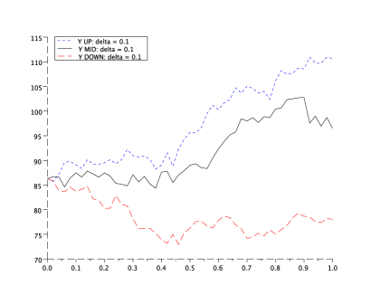
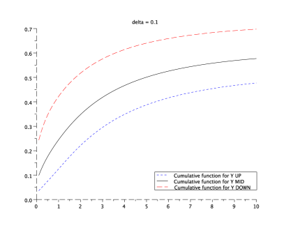
Figure 1: ("Black Scholes example") Three trajectories for the observation process $Y$ and for $\delta=0.1$ (on the left), and the corresponding cumulative functions $\mathds{P}(\tau^{\bar{X}}_{\bf a}\leq t_{n}|Y_{t_{0}},\ldots,Y_{t_{m}})$ with $t_{m}=1$ and $t_{n}\in[1.1,11]$ years (on the right).

Figure 2: ("Black Scholes example") Left graphics corresponds to three trajectories for the observation process $Y$, for $\delta=0.1$ (Y UP), $\delta=0.3$ (Y MID), $\delta=0.5$ (Y DOWN), and the right hand side graphics correspond to a zoom of the cumulative functions $\mathds{P}(\tau^{\bar{X}}_{\bf a}\leq t_{n}|Y_{t_{0}},\ldots,Y_{t_{m}})$ with $t_{m}=1$ and $t_{n}\in[1.1,11]$ years.

Example 4 (The Ornstein-Uhlenbeck example).

In the second model, we suppose that both the signal and the observation process evolve following the Ornstein-Uhlenbeck dynamics:

$$\begin{cases}dX_{t}=\lambda(\theta-X_{t})dt+\sigma dW_{t},&X_{0}=x_{0},\\ dY_{t}=\lambda(\theta-Y_{t})dt+\sigma dW_{t}+\delta d\widetilde{W}_{t},&Y_{0}=y_{0}\end{cases}$$ (50)

or setting $Z_{t}=Y_{t}-X_{t}$

$$dZ_{t}=-\lambda Z_{t}dt+\delta d\widetilde{W}_{t},$$

meaning that $Z$ is still an Ornstein-Uhlenbeck process with mean value $\theta=0$ and with volatility $\delta.$ The parameters are chosen as follows: $\lambda=0.18$, $\theta=0.35$, $\sigma=0.12$, $x_{0}=y_{0}=0.35$ (as in [3]) and ${\bf a}=0.2$. The numerical results are represented in Figure 3 where we depict three trajectories of the observation process $Y$ for $\delta=0.16$ (left hand side graphics of Figure 3) and the associated cumulative functions $\mathds{P}(\tau^{\bar{X}}_{\bf a}\leq t_{n}|Y_{t_{0}},\ldots,Y_{t_{m}})$, with $t_{m}=1$ and $t_{n}\in[1.1,6]$ in years (right hand side graphics of Figure 3). Once again, we remark that, as in the "Black Scholes example", for a fixed time $t_{n}$, the lower the trajectory is, the higher its probability is to hit the barrier.

In this example, the function $\bar{F}(t_{m},t_{n},\cdot)$ has been computed using Monte Carlo simulations of size $M=10^{5}$(see the formula (45)) with $50$ discretization steps over $[t_{m},t_{n}]$. The computation time to get one cumulative function $\mathds{P}(\tau^{\bar{X}}_{\bf a}\leq t_{n}|Y_{t_{0}},\ldots,Y_{t_{m}})$ for a given $t_{n}$ is about $6.5$ minutes.

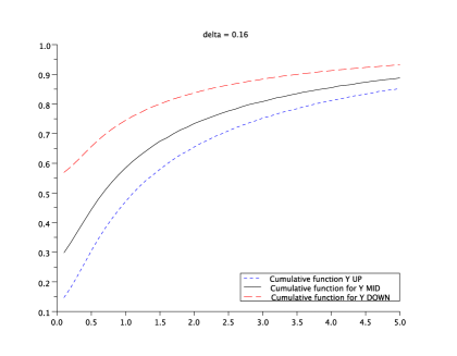
Figure 3: ("Ornstein-Uhlenbeck example") Left graphics correspond to three trajectories for the observation process $Y$, for $\delta=0.16$ and the right hand side graphics correspond to the cumulative functions $\mathds{P}(\tau^{\bar{X}}_{\bf a}\leq t_{n}|Y_{t_{0}},\ldots,Y_{t_{m}})$ with $t_{m}=1$ and $t_{n}\in[1.1,6]$ years.

References

• [1] J. A. Bucklew and G. L. Wise. Multidimensional asymptotic quantization theory with $r$-th power distribution measures. IEEE Trans. Inform. Theory, 28:239-247, 1982.
• [2] G. Callegaro, A. Sagna. An application to credit risk of optimal quantization methods for non- linear filtering. The Journal of Computational Finance, 2012. To appear.
• [3] D. Coculescu, H. Geman, and M. Jeanblanc. Valuation of default sensitive claims under imperfect information. Finance and Stochastics, 12(2):195-218, 2008.
• [4] D. Duffie and D. Lando. Term structures of credit spreads with incomplete accounting information. Econometrica, 69(3):633-664, 2001.
• [5] A. Gersho and R. Gray. Vector Quantization and Signal Compression. Kluwer Academic Press, Boston, 1992.
• [6] P. Glasserman, P. Heidelberger, and P. Shahabuddin. Asymptotically optimal importance sampling and stratification for pricing path-dependent options. Mathematical Finance, 9:117-152, 1999.
• [7] E. Gobet. Schémas dÕEuler pour diffusion tuée. Application aux options barrière. PhD thesis, Université Denis Diderot - Paris VII, 1998.
• [8] S. Graf and H. Luschgy. Foundations of Quantization for Probability Distributions. Lect. Notes in Math. 1730, 2000.
• [9] H. Luschgy and G. Pagès. Functional quantization of a class of Brownian diffusions: A constructive approach. Stochastic Processes & Their Applications, 116:310-336, 2006.
• [10] G. Pagès. A space quantization method for numerical integration. Journal of Computational and Applied Mathematics, 89:1-38, 1998.
• [11] G. Pagès and H. Pham. Optimal quantization methods for nonlinear filtering with discrete time observations. Bernoulli, 11(5):893-932, 2005.
• [12] G. Pagès and J. Printems. Optimal quadratic quantization for numerics: the gaussian case. Monte Carlo Methods and Applications, 9(2):135-165, 2003.
• [13] G. Pagès and J. Printems. Functional quantization for numerics with an application to option pricing. Monte Carlo Methods and Applications, 11(4):407-446, 2005.
• [14] A. Sagna. Pricing of barrier options by marginal functional quantization method. Monte Carlo Methods and Applications, 17(4), 2012.
• [15] P. Zador. Asymptotic quantization error of continuous signals and the quantization dimension. IEEE Trans. Inform. Theory, 28:139-149, 1982.