Storing Cycles in Hopfield-type Networks with Pseudoinverse Learning Rule: Admissibility and Network Topology

Abstract

Cyclic patterns of neuronal activity are ubiquitous in animal nervous systems, and partially responsible for generating and controlling rhythmic movements such as locomotion, respiration, swallowing and so on. Clarifying the role of the network connectivities for generating cyclic patterns is fundamental for understanding the generation of rhythmic movements. In this paper, the storage of binary cycles in Hopfield-type and other neural networks is investigated. We call a cycle defined by a binary matrix $\Sigma$ admissible if a connectivity matrix satisfying the cycle’s transition conditions exists, and if so construct it using the pseudoinverse learning rule. Our main focus is on the structural features of admissible cycles and the topology of the corresponding networks. We show that $\Sigma$ is admissible if and only if its discrete Fourier transform contains exactly $r=\mathrm{rank}(\Sigma)$ nonzero columns. Based on the decomposition of the rows of $\Sigma$ into disjoint subsets corresponding to loops, where a loop is defined by the set of all cyclic permutations of a row, cycles are classified as simple cycles, and separable or inseparable composite cycles. Simple cycles contain rows from one loop only, and the network topology is a feedforward chain with feedback to one neuron if the loop-vectors in $\Sigma$ are cyclic permutations of each other. For special cases this topology simplifies to a ring with only one feedback. Composite cycles contain rows from at least two disjoint loops, and the neurons corresponding to the loop-vectors in $\Sigma$ from the same loop are identified with a cluster. Networks constructed from separable composite cycles decompose into completely isolated clusters. For inseparable composite cycles at least two clusters are connected, and the cluster-connectivity is related to the intersections of the spaces spanned by the loop-vectors of the clusters. Simulations showing successfully retrieved cycles in continuous-time Hopfield-type networks and in networks of spiking neurons exhibiting up-down states are presented.

1 Introduction

Applications of artificial neural networks in content addressable (associative) memory have attracted much attention in the last few decades (Hopfield82; Hopfield84; Little; Capacity; Universal; Associative). Hopfield-type networks are among the most popular models of artificial neural networks for studying content addressable memory. According to Hopfield’s original idea, the privileged regime to store information has been fixed point attractors, however experiments (e.g., ChaosBrain) indicate that cycles are used to store information and chaotic dynamics appears as the background regime composed of these cyclic “memory bags”.

In general, the storage of pattern sequences is one of the most important tasks in both biological and artificial intelligence systems. A sequence containing repetitions of the same subsequence is said to be complex (Guyon; WangArbib90; Wang03), and cyclic patterns (or cycles of patterns) are one of the important classes of such sequences. In animal nervous systems, cyclic patterns of neuronal activity are ubiquitous and partially responsible for generating and controlling rhythmic movements such as locomotion, respiration, swallowing and so on. Neural networks that can produce cyclic patterned outputs without rhythmic sensory or central input are called central pattern generators (CPGs). While in some lower level invertebrate animals detailed connectivity diagrams among identified CPG neurons have been experimentally determined, the anatomic structure of CPG networks in most higher vertebrate animals including human beings remain largely unknown (e.g., MackayLyons02; Marder05; Selverston10).

According to Yuste (Yuste08), the network connectivity problem, i.e. experimentally identifying the connectivity diagram of biological neural networks, is one of the four basic problems that have to be solved to fully understand a biological neural network. However, recent experimental observations (e.g., Dickinson92; Meyrand94) suggested that CPGs may be highly flexible, some of them may even be temporarily formed only before the production of motor activity (Jean01). This makes experimentally identifying the architecture of CPGs very difficult. As indirect approaches to solve the network connectivity problem, observable movement features such as symmetry etc. have been used to infer aspects of CPG structures (e.g. Golubitsky99). In this paper, we study the network connectivity problem for storing binary cyclic patterns. Given an arbitrary binary cyclic pattern, we ask whether there exists a network whose architecture allows to produce it, and if there exists one, then how the cycle determines the network structure. While the main motivation for our study is the storage of cycles in continuous-time Hopfield-type networks, this question is independent of the specific dynamics of the individual neurons the network is composed of.

In both discrete and continuous asymmetric variants of Hopfield-type networks, the storage and retrieval of sequences including cycles of binary patterns have been investigated (Personnaz; Guyon; Gencic90), and biologically plausible learning rules such as Hebb’s rule, the pseudoinverse rule and their variants with and without delays have been used. In this paper, we follow Gencic90 and use continuous-time Hopfield-type networks as models to study the relation between cyclic patterns and the architecture of the networks constructed from them. In addition to the simple dynamics of single neurons, another advantage of Hopfield-type networks is that they deal with binary states. In neurophysiology it is well known that both CPG neurons and cortical neurons show bistable membrane behaviors, which are commonly referred to as plateau potentials (e.g Straub02; Grillner03; Selverston10) or up-down states (e.g. Sanchez00; Cossart03). Accordingly, a sequence of the binary states $+1$ and $-1$ traversed by a single neuron in a Hopfield-type network can be interpreted as a sequence of up and down states, respectively.

While simulations of networks constructed using Hebbian learning rules have been shown to be qualitatively consistent with experimental recordings (Kleinfeld88), it is well known that Hopfield-type networks with Hebbian learning rules do not perform well when the patterns to be stored are correlated which is usually the case in practice (HebShort1). To avoid this problem, a pseudoinverse learning rule was introduced by Amari (Amari77), and in the Hopfield framework by Personnaz et al. and Kanter et al. (Personnaz; Sompolinsky87). It has been suggested that the pseudoinverse learning rule and its variants may take key roles in the associative perception of human faces in the human cortex (Prosopagnosia00) and the encoding of location information in the rat hippocampus (Marinaro07). Recently, Tapson and Schaik proposed an algorithm referred to as OPIUM (Online Pseudoinverse Update Method) for computing the pseudoinverse, and showed that the pseudoinverse learning rule is plausible as a physiological process in real neurons (TapsonSchaik13). Since the pseudoinverse method gives an exact solution of the network connectivity problem if a solution exists (Personnaz), we use this method to construct networks for storing binary cycles.

Although the pseudoinverse rule and its variants (Amari77; Personnaz) extend to more general cases, most investigations in discrete-time Hopfield-type networks characterized or were implemented for cycles or sequences of linearly independent patterns (e.g. Personnaz; Sompolinsky87). An approach to storing cycles of correlated as well as linearly independent patterns in continuous-time Hopfield-type networks has been proposed by Gencic90. In this study, a successfully retrieved cycle is revealed as an attracting limit cycle in the network dynamics, but the question for which cycles the corresponding network connectivity problem admits a solution was not addressed.

In our study, a cycle is defined by a $N\times p$-matrix, $\Sigma$, of binary states, where $N$ is the number of neurons in the network and $p$ is the length of the cycle. The network connectivity problem associated with a cycle $\Sigma$ can be formulated as follows: Find a real $N\times N$-matrix $\mathbf{J}$ such that $\mathbf{J}\Sigma=F$, where $F$ is related to $\Sigma$ by a cyclic permutation of the columns. The main objective of this paper is to study the existence and properties of solutions of this equation along with the structural features of the corresponding cycles, and the network topologies associated with them. If a solution $\mathbf{J}$ exists, we call the cycle $\Sigma$ admissible and construct $\mathbf{J}$ using the pseudoinverse method.

While the main motivation for our study is the storage of binary cycles in continuous-time Hopfield-type neural networks, the question whether a given cycle is admissible is independent of the particular network-model. For the discrete-time Hopfield-type networks studied by Personnaz and Guyon, $\mathbf{J}$ can be used directly as connectivity matrix. For the continuous-time Hopfield-type networks considered in Section 2.1, we follow the approach of Gencic90 and represent the connectivity matrix as a weighted sum of $\mathbf{J}$ and another matrix $\mathbf{J^{0}}$, that serves to store the individual patterns in $\Sigma$ as fixed points. To demonstrate that our approach also works for more complicated neuron-models, we introduce in Section 2.2 a single-compartment neuron model that exhibits up-down states and show an example of a successfully retrieved cycle.

Our main objective is to analyze and classify the structural features of admissable cycles $\Sigma$ and the topology of the networks constructed from them. A basic result is that if and only if the discrete Fourier transform of $\Sigma$ contains exactly $r=\mathrm{rank}(\Sigma)$ nonzero columns, then $\Sigma$ is admissible.

Our approach to classify cycles is based on the decomposition of the row vectors of $\Sigma$ into disjoint subsets corresponding to different loops created by cyclic permutations of the rows. If the cycle is admissible, each of these loops is associated with an invariant subspace of the row space, $\mathcal{U}$, of $\Sigma$ under cyclic permutations. This row-decomposition leads naturally to a classification of cycles into simple cycles, separable composite cycles, and inseparable composite cycles. Simple cycles contain rows from a single loop only. Composite cycles contain rows from at least two disjoint loops, and for each loop the neurons corresponding to the loop vectors in $\Sigma$ are identified with a cluster, which in turn corresponds to an indecomposable invariant subspace of $\mathcal{U}$ under cyclic permutations if $\Sigma$ is admissible. Two clusters are directly connected if their subspaces intersect nontrivially, and they are connected if they are part of a chain of directly connected clusters. A network constructed from a simple admissible cycle has only one cluster, and we show that the network topology is a feedforward chain with feedback to one neuron if the loop vectors in $\Sigma$ are all cyclic permutations of each other. For special simple cycles, there is only one feedback and the network topology simplifies to a ring. Networks constructed from separable composite cycles decompose into completely isolated clusters.

The paper is organized as follows. In Section 2, the pseudoinverse learning rule is introduced in the framework of continuous-time Hopfield-type networks. Additionally, in order to demonstrate that the pseudoinverse learning rule can be applied to other networks as well, networks of spiking neurons with plateau membrane potentials and postinhibitory rebound are introduced, and simulations showing the successful retrieval of a prescribed cycle are presented. In Section 3, the general admissibility criterion in terms of the discrete Fourier transform of the cycle matrix is formulated and proved, and the relation of admissible cycles with cyclic permutation groups is discussed. Based on the structural features of the invariant subspaces of the row space of an admissible cycle, in Section 4, admissible cycles are classified into simple cycles, and separable and inseparable composite cycles, and for each type of cycles a corresponding admissibility condition is derived. In Section 5, the topologies of networks constructed from different types of admissible cycles are studied, and in Section 6 implications of the results presented in this paper are discussed.

2 Pseudoinverse Learning Rule and Neural Networks

2.1 Hopfield-type Neural Networks

A continuous-time Hopfield-type network (Hopfield84) is described by a system of ordinary differential equations for $u_{i}(t)$, $1\leq i\leq N$, which model the membrane potential of the $i$-th neuron in the network at time $t$. Assuming that all neurons are identical, normalizing the neuron amplifier input capacitance and resistance to unity and neglecting external inputs, the governing equations are,

$$\frac{du_{i}}{dt}=-u_{i}+\sum\limits_{j=1}^{N}\tilde{J}_{ij}v_{j}\mbox{, }1\leq i\leq N,$$ (1)

where $v_{j}(t)$ is the firing rate of the $j$-th neuron and $\mathbf{\tilde{J}}=(\tilde{J}_{ij})_{N\times N}$ is the connectivity matrix. The firing rate $v_{j}$ is related to the membrane potential $u_{j}$ through a sigmoid-shaped gain function, $v_{j}=g(u_{j})$, which we choose, following Hopfield84, as $g(u_{j})=\tanh(\lambda u_{j})$, where $\lambda$ controls the steepness. Using vector notation, $\mathbf{u}=(u_{1},\dots,u_{N})^{T}$, $\mathbf{v}=(v_{1},\dots,v_{N})^{T}$, (1) can be more compactly written as (dots denote time derivatives)

$$\dot{\mathbf{u}}=-\mathbf{u}+\tilde{\mathbf{J}}\tanh(\lambda\mathbf{u}),$$ (2)

where here and subsequently a scalar function applied to a vector or matrix denotes the vector or matrix obtained by applying the function to each component, i.e.

$$\tanh(\lambda\mathbf{u})=(\tanh(\lambda u_{1}),\tanh(\lambda u_{2}),\dots,\tanh(\lambda u_{N}))^{T}.$$

Alternatively, since $u_{j}=\mathrm{arctanh}(v_{j})/\lambda$, (2) can be rewritten as a system of differential equations for the firing rates,

$$\dot{\mathbf{v}}=\lambda(I-\mathrm{diag}(\mathbf{v}^{2}))(\tilde{\mathbf{J}}\mathbf{v}-\frac{\mathrm{arctanh}(\mathbf{v})}{\lambda}),$$ (3)

where $I$ is the $N\times N$ identity matrix.

In this paper we study the structure of binary pattern cycles that can be stored in the network modeled by the above autonomous system. Following Hopfield82; Hopfield84, any $N$-dimensional $\{-1,1\}$-valued column vector is identified with a binary vector or pattern, and we use $+$ and $-$ to denote $1$ and $-1$.

Personnaz and Guyon studied the storage of sequences of patterns in discrete-time Hopfield-type networks. A sequence of $p$ patterns $\xi^{(\mu)}=(\xi_{1}^{(\mu)},\xi_{2}^{(\mu)},\dots,\xi_{N}^{(\mu)})^{T}$, $1\leq\mu\leq p$, $\xi_{i}^{(\mu)}=+\mbox{ or }-$, is defined by $p$ transition conditions $\xi^{(\mu)}\rightarrow f^{(\mu)}$, where $f^{(\mu)}$ is one of the given vectors, i.e., $f^{(\mu)}\in\{\xi^{(1)},\dots,\xi^{(p)}\}$ for each $\mu$. Thus a sequence is characterized by two $N\times p$-matrices $\Sigma=(\xi^{(1)},\dots,\xi^{(p)})$ and $F=(f^{(1)},\dots,f^{(p)})$. The two matrices are related to each other by the transition conditions, which can be conveniently formulated in terms of a $p\times p$ transition matrix as $F=\Sigma\mathbf{P}$, where $\mathbf{P}_{\nu\mu}=1$ if $f^{(\mu)}=\xi^{(\nu)}$ and $0$ otherwise. For example, for $p=3$ and the simplest case of a sequence starting at $\xi^{(1)}$ and terminating at $\xi^{(3)}$, $\xi^{(1)}\rightarrow\xi^{(2)}$, $\xi^{(2)}\rightarrow\xi^{(3)}$, $\xi^{(3)}\rightarrow\xi^{(3)}$, we have $F=(\xi^{(2)},\xi^{(3)},\xi^{(3)})$ and $P$ is singular, but the general definition in terms of $\Sigma$ and $F$ allows to consider more complex as well as multiple sequences. Personnaz showed that the storage of such a sequence leads to the matrix equation,

$$\mathbf{J}\Sigma=F,$$ (4)

for the connectivity matrix $\mathbf{J}$ of the discrete network. It was pointed out by Personnaz, that, if $F\Sigma^{+}\Sigma=F$, where $\Sigma^{+}$ is the Moore-Penrose pseudoinverse of $\Sigma$, then (4) has the exact solution $\mathbf{J}=F\Sigma^{+}$, which was called associating learning rule by these authors.

A cycle of $p$ patterns is a sequence with $F=(\xi^{(2)},\xi^{(3)},\dots,\xi^{(p)},\xi^{(1)})$, i.e., $\xi^{(\mu)}\rightarrow\xi^{(\mu+1)}$ for $\mu<p$ and $\xi^{(p)}\rightarrow\xi^{(1)}$, and the corresponding transition matrix is

$$\mathbf{P}=\left(\begin{array}[]{rrrrrr}0&0&0&\cdots&0&1\\ 1&0&0&\cdots&0&0\\ 0&1&0&\cdots&0&0\\ \vdots&\vdots&\vdots&\ddots&\vdots&\vdots\\ 0&0&0&\cdots&0&0\\ 0&0&0&\cdots&1&0\end{array}\right).$$ (5)

We are interested in the storage of cycles in the continuous-time Hopfield networks defined by (2). Our approach to compute a connectivity matrix $\mathbf{\tilde{J}}$ for this purpose follows Gencic90. In this paper, the connectivity matrix $\mathbf{\tilde{J}}$ is decomposed as

$$\mathbf{\tilde{J}}=\beta_{K}(C_{0}\mathbf{J^{0}}+C_{1}\mathbf{J}),$$ (6)

where $\mathbf{J^{0}}$ serves to stabilize the network in its current memory state and $\mathbf{J}$ imposes the transitions between the memory states. Here, $C_{1}=1-C_{0}$ and $C_{0}$, $0\leq C_{0}\leq 1$, control the relative contributions of the two components of $\mathbf{\tilde{J}}$. The fixed point condition is realized by requiring that $\mathbf{v}=\beta_{1}\xi^{(\mu)}$, with a parameter $0<\beta_{1}<1$, is a fixed point if $C_{0}=1$. Noting that $\mathrm{arctanh}(x)$ is an odd function and $|\xi^{(\mu)}_{i}|=1$, this leads, according to (3), to the condition

$$\mathbf{\tilde{J}}\beta_{1}\xi^{(\mu)}=\frac{1}{\lambda}\mathrm{arctanh}(\beta_{1}\xi^{(\mu)})=\frac{1}{\lambda}\mathrm{arctanh}(\beta_{1})\xi^{(\mu)},$$

for every $\mu$, hence $\mathbf{\tilde{J}}\Sigma=\beta_{K}\Sigma$ with $\displaystyle{\beta_{K}=\frac{1}{\lambda\beta_{1}}\mathrm{arctanh}(\beta_{1})}$, which has the solution $\mathbf{\tilde{J}}=\beta_{K}\mathbf{J^{0}}$ with

$$\mathbf{J^{0}}=\Sigma\Sigma^{+}.$$ (7)

Regarding the transition conditions, we stipulate that $\mathbf{v}(t)=\beta_{1}\xi^{(\mu)}$ implies $\mathbf{v}(t+\tau)=\beta_{1}f^{(\mu)}$ for some $\tau$, and require accordingly for $C_{0}=0$ that $\mathbf{\tilde{J}}\Sigma=\beta_{K}F$. This leads to equation (4), which in terms of the transition matrix $\mathbf{P}$, equation (5), becomes

$$\mathbf{J}\Sigma=\Sigma\mathbf{P}.$$ (8)

According to the associating learning rule of Personnaz, (8) has the solution

$$\mathbf{J}=\Sigma\mathbf{P}\Sigma^{+},$$ (9)

provided that $\Sigma\mathbf{P}\Sigma^{+}\Sigma=\Sigma\mathbf{P}$. If this condition is not satisfied, (8) has no solution.

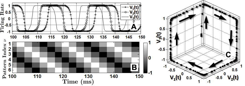
Figure 1: A successfully retrieved cycle $\Sigma$ (see text for details) in a network of three neurons. A shows the firing rates $v_{i}(t)$ of the three neurons and the raster plot B shows the overlaps $m^{(\nu)}(t)$, which measure the similarity of the network state $\mathbf{v}(t)$ with each of the six patterns in the cycle (see text). C illustrates the retrieval of the cycle in the phase space of the system.

The main objective of this paper is the study of the existence and properties of the solutions of (8) along with the structural features of the corresponding cycles, and the network topologies resulting from $\mathbf{J^{0}}$ and $\mathbf{J}$ defined by (7) and (9). A bifurcation analysis and a study of the dynamics of (2) with (6), with $C_{0}$ and $\beta=\lambda\beta_{K}>1$ treated as parameters, are given elsewhere, where we also consider the extension of (2) to a dynamical system with a delay,

$$\dot{\mathbf{u}}=-\mathbf{u}+C_{0}\beta_{K}\mathbf{J^{0}}\tanh(\lambda\mathbf{u})+C_{1}\beta_{K}\mathbf{J}\tanh(\lambda\mathbf{u}_{\tau}),$$ (10)

with a delay-time $\tau>0$ and $\mathbf{u}_{\tau}(t)=\mathbf{u}(t-\tau)$. Here we show only one example of a successfully retrieved cycle for (2), a network of $N=3$ neurons. The cycle consists of six states, $\Sigma=(\xi^{(1)},\dots,\xi^{(6)})$, with $\xi^{(1)}=(+,+,+)^{T}$, $\xi^{(2)}=(+,+,-)^{T}$, $\xi^{(3)}=(+,-,-)^{T}$ and $\xi^{(3+\mu)}=-\xi^{(\mu)}$ for $\mu=1,2,3$. The retrieval of the cycle is illustrated in Figure 1. The raster plot B in this figure shows the overlaps, defined in general as

$$m^{(\nu)}(t)=\frac{1}{N}\sum\limits_{i=1}^{N}v_{i}(t)\xi_{i}^{(\nu)}\mbox{, }1\leq\nu\leq p,$$ (11)

of the actual network state $\mathbf{v}(t)$ with the patterns of the cycle. The overlap $m^{(\nu)}(t)$ is a normalized measure of the similarity of $\mathbf{v}(t)$ with $\xi^{(\nu)}$. Maximal similarity with $\xi^{(\nu)}$ and $-\xi^{(\nu)}$ occurs for $m^{(\nu)}$ close to $1$ and $-1$, respectively. The raster plot of the overlaps in Figure 1B as well as the time series in Figure 1A clearly illustrate that the cycle is retrieved successfully. The parameters $C_{0}$ and $\beta$ used in this simulation were $C_{0}=0.6$ and $\beta=4$.

2.2 Networks of Spiking Neurons

As was pointed out in the introduction, although our results are developed in the framework of Hopfield-type networks, they also can be used to store cycles in other neural networks. In this subsection, we introduce a network model of identical spiking neurons with bistable membrane behavior and postinhibitory rebound, and show an example of a successfully retrieved cycle in a network constructed using the pseudoinverse method.

We consider the simplest single-compartment neuron model, the passive integrate-and-fire (PIF) model (DayanAbbott01; Abbott07). The model is described by the following first-order nonlinear ordinary differential equation,

$$c_{m}\frac{dV_{i}}{dt}=-I_{L}^{(i)}(t)-I_{nl}^{(i)}(t)+I_{{}_{synE}}^{(i)}(t)+I_{{}_{synI}}^{(i)}(t),$$ (12)

where $V_{i}(t)$ is the membrane potential of the $i$-th neuron in the network, and if $V_{i}(t)\geq\theta$ where $\theta=-45\mathrm{mV}$ is the threshold for the firing action potentials, then $V_{i}(t+dt)=0$, and $V_{i}(t+2dt)=V_{reset}$ with $dt=0.005\mathrm{ms}$ and $V_{reset}=-55\mathrm{mV}$. After each action potential, an absolute refractory period $t_{Refr}=1\mathrm{ms}$ is imposed, and during the refractory period the membrane potential $V_{i}(t)$ is fixed at $V_{reset}$. The parameter $c_{m}$, chosen as $c_{m}=20\mathrm{nF/mm^{2}}$, is the specific membrane capacitance. The membrane and synaptic currents of the $i$-th neuron are respectively given as follows.

Leakage membrane current:

$$I_{L}^{(i)}(t)=g_{L}(V_{i}(t)-E_{L}),$$ (13)

where $g_{L}=1\mathrm{\mu S/mm^{2}}$ and $E_{L}=-68\mathrm{mV}$.

Nonlinear membrane current:

$$I_{nl}^{(i)}(t)=g_{nl}(V_{i}(t)-E_{1})(V_{i}(t)-E_{2})(V_{i}(t)-E_{3})-\delta,$$ (14)

where $g_{nl}=0.03\mathrm{mV^{-2}}$, $E_{1}=-72\mathrm{mV}$, $E_{2}=-58\mathrm{mV}$, $E_{3}=-44\mathrm{mV}$ and $\delta$ is a parameter for shifting the nonlinear membrane current to control the stability of the up state. In the simulation shown in the paper, we chose $\delta=-31.685$.

Excitatory synaptic current:

$$I_{{}_{synE}}^{(i)}(t)=\bar{g}_{{}_{synE}}s_{i}(t)(V_{i}(t)-E_{{}_{synE}}),$$ (15)

where $\bar{g}_{{}_{synE}}=68\mathrm{\mu S/mm^{2}}$, $E_{{}_{synE}}=-120\mathrm{mV}$, and the activation variable $s_{i}(t)$ satisfies the following first order differential equation,

$$\frac{ds_{i}}{dt}=\alpha_{E}\Big{(}s_{i}-10\sum\limits_{j=1}^{N}\Theta(J_{ij})J_{ij}\Theta(V_{j}(t-\tau)-V_{thr})\Big{)},$$ (16)

where $\alpha_{E}=1$, $V_{thr}=-45\mathrm{mV}$, $\tau=10\mathrm{ms}$, $\Theta(x)$ is the Heaviside step function, and the $J_{ij}$ are the components of the connectivity matrix $\mathbf{J}$.

Inhibitory synaptic current:

$$I_{{}_{synI}}^{(i)}(t)=\bar{g}_{{}_{synI}}z_{i}(t)(V_{i}(t)-E_{{}_{synI}}),$$ (17)

where $\bar{g}_{{}_{synI}}=118\mathrm{\mu S/mm^{2}}$, $E_{{}_{synI}}=-120\mathrm{mV}$, and the activation variable is given by $z_{i}(t)=(x_{i}(t)+y_{i}(t))/2$, with $x_{i}(t)$ and $y_{i}(t)$ satisfying the following first order differential equations,

$$\begin{array}[]{l}\displaystyle{\frac{dx_{i}}{dt}}=\alpha_{I}\Big{(}x_{i}-10\sum\limits_{j=1}^{N}\Theta(-J_{ij})J_{ij}\Theta(V_{j}(t-\tau)-V_{thr})\Big{)},\\ \displaystyle{\frac{dy_{i}}{dt}}=\beta_{I}\Big{(}y_{i}+10\sum\limits_{j=1}^{N}\Theta(-J_{ij})J_{ij}\Theta(V_{j}(t-\tau)-V_{thr})\Big{)},\end{array}$$ (18)

with $\alpha_{I}=2$, $\beta_{I}=0.08$, and $\tau=10\mathrm{ms}$.

With the parameters of a single neuron fixed as above, the dynamics of a network of $N$ PIF-neurons is fully determined by the connectivity matrix $\mathbf{J}$. We constructed $\mathbf{J}$ from prescribed cycles using the pseudoinverse learning rule $\mathbf{J}=\Sigma\mathbf{P}\Sigma^{+}$, i.e. without invoking a fixed point condition. Figure 2 illustrates a successfully retrieved $6\times 8$ cycle $\Sigma$. The first four rows of $\Sigma$ are $\sigma_{1}\mathbf{P}^{j-1}$, $j=1,2,3,4$, and the last two rows are $\sigma_{2}$ and $\sigma_{2}\mathbf{P}$, where $\sigma_{1}=(+,+,+,+,-,-,-,-)$ and $\sigma_{2}=(+,+,-,-,+,+,-,-)$.

Figure 2A shows the retrieved traces of the membrane potentials $V_{i}(t)$ of the six neurons in the network. Since the firing rates are not included as variables in the model, they have to be extracted from the time series. Following DayanAbbott01, we counted for given $t$ the number of times $t^{\prime}$ within the time window $t-\Delta t/2\leq t^{\prime}\leq t+\Delta t/2$ at which neuron $i$ fired, and divided this number by $\Delta t$. The resulting function, $R_{i}(t)$, is considered as an approximation of the firing rate of the $i$-th neuron. For $\Delta t$ we chose $\Delta t=5\mathrm{ms}$. We also introduce the normalized firing rates, $v_{i}(t)=2R_{i}(t)/\max R_{i}(t)-1$ (so that $-1\leq v_{i}(t)\leq 1$, analogous to the firing rates used in continuous-time Hopfield-type networks), and define the overlaps $m^{(\nu)}(t)$ as in equation (11).

To compare the membrane potentials with the prescribed cycle, we extracted the time spans between the first spike and the last spike in each up-state, and identified their average divided by 4 as the time span for each binary state. The resulting time span is $11.3\mathrm{ms}$ and is slightly larger than the time-delay $\tau=10\mathrm{ms}$ in the synaptic couplings. In Figure 2A, the gray strips in the background indicate these time spans, and the dark gray $+$’s and $-$’s label the corresponding binary states in the prescribed cycle. The firing rates $R_{i}(t)$ and the overlaps $m^{(\nu)}(t)$ are displayed in Figure 2B and C, respectively. The black arrows in A, B, and C indicate the time span when the first binary pattern, $\xi^{(1)}=(+,+,+,+,+,+)^{T}$, in the prescribed cycle is retrieved for the first time in the displayed time range. The plots in Figure 2 clearly demonstrate that the cycle is retrieved successfully.

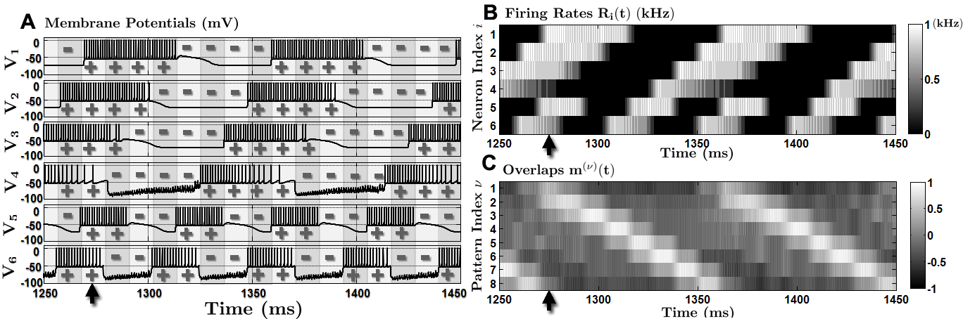
Figure 2: Successful retrieval of a cycle $\Sigma$ with eight states prescribed in a network of six spiking neurons with the pseudoinverse learning rule. A: membrane potential, B: Firing rates, and C: Overlaps (see text for details).

Other cycles were retrieved successfully as well, but in contrast to continuous time Hopfield-type networks, especially with delayed couplings, we observed in simulations that some prescribed cycles are difficult to be retrieved in networks of the spiking neurons introduced in this subsection. This is likely because of the complicated dynamics of the individual neurons, which makes the appropriate choice of parameter values more difficult. In general, especially in physiologically based neural network models, the neuronal dynamics may take key roles in shaping the dynamics of the networks, and reinforce or weaken the contribution of the network structure in reproducing prescribed cycles. In this case, it is important to find out whether a cyclic patterned output in a system arises from a network-based mechanism or not, and if it does, then to which extent and how the cyclic patterned output is determined by the network architecture.

In the next three sections, without considering the specific dynamics of single neurons, we formulate and prove conditions for any cyclic pattern under which a connectivity matrix in accordance with the cycle’s transition conditions can be constructed, and for cycles for which this is the case we analyze and classify their structural features and their relation to the network topology.

3 Admissible Cycles and Cyclic Permutation Groups

Definition 1.

Let $\mathbf{P}$ be the cyclic $p\times p$-permutation matrix defined in (5). A cycle defined by a binary $N\times p$-matrix $\Sigma=(\xi^{(1)},\xi^{(2)},\dots,\xi^{(p)})$ is said to be admissible, if there is a real $N\times N$ matrix $\mathbf{J}$ such that equation (8) is satisfied.

Note that if $\Sigma$ is admissible, the solution to (8) may be not unique. If there are several solutions, we select (9) as distinguished solution because of its close relationship to $\mathbf{J^{0}}$, see Remark 1(b) below.

Gencic90 consider a special type of cycles defined by $p$ binary vectors $\Sigma^{\prime}=(\xi^{(1)},\xi^{(2)},\dots,\xi^{(p)})$, which satisfy the transition condition $\xi^{(1)}\rightarrow\xi^{(2)}\rightarrow\cdots\xi^{(p)}\rightarrow-\xi^{(1)}\rightarrow-\xi^{(2)}\rightarrow\cdots-\xi^{(p)}\rightarrow\xi^{(1)}$. In this paper we consider these cycles as special cases of cycles of period $2p$ with $\Sigma=(\Sigma^{\prime},-\Sigma^{\prime})$.

For storing sequences, Personnaz pointed out that, if the associating learning rule $F\Sigma^{+}\Sigma=F$ is satisfied, the rows of $F$ are linear combinations of the rows of $\Sigma$. This follows from the fact that $\Sigma^{+}\Sigma$ is the orthogonal projection matrix onto the subspace of $\mathbb{R}^{p}$ spanned by the rows of $\Sigma$. For storing single cycles, their conclusion can be reformulated geometrically as follows: