An efficient multigrid calculation of the Far Field map for Helmholtz and Schrödinger equations

Abstract

In this paper we present a new highly efficient calculation method for the far field amplitude pattern that arises from scattering problems governed by the $d$-dimensional Helmholtz equation and, by extension, Schrödinger’s equation. The new technique is based upon a reformulation of the classical real-valued Green’s function integral for the far field amplitude to an equivalent integral over a complex domain. It is shown that the scattered wave, which is essential for the calculation of the far field integral, can be computed very efficiently along this complex contour (or manifold, in multiple dimensions). Using the iterative multigrid method as a solver for the discretized damped scattered wave system, the proposed approach results in a fast and scalable calculation method for the far field map. The complex contour method is successfully validated on Helmholtz and Schrödinger model problems in two and three spatial dimensions, and multigrid convergence results are provided to substantiate the wavenumber scalability and overall performance of the method.

1 Introduction

Scattering problems are of key importance in many areas of science and engineering since they carry information about an object of interest over large distances, remote from the given target. Consequently, ever since their original statement a variety of applications of scattering problems have arisen in many different scientific subdomains. In chemistry and quantum physics, for example, virtually all knowledge about the inner workings of a molecule has been obtained through scattering experiments [31]. Similarly, in many real-life electromagnetic or acoustic scattering problems information about a far away object is obtained through radar or sonar [13], intrinsically requiring the solution of 2D or 3D wave equations.

The near- and far field of a scattering problem are specific regions in space identified by the distance from the scattering object. In these regions the scattering solution is subject to certain physical and mathematical properties. In the far field, the solution behaves as a spherical outgoing wave with an amplitude that decays as $1/r$, where $r$ is the distance to the scattering object. In this regime, the (asymptotic) solution can be written as a product of an angular part and a radial part. The near field is the region just outside the scattering object, where the solution has not yet reached its asymptotic form. In electromagnetic scattering, for example, the near field is dominated by dipole terms. Predicting the near- and far field solution is important for many present-day industrial applications (e.g. radar), but also plays a key role in physical measurement systems such as tomography, near field microscopy and MRI.

However, far field maps are not limited to 2D or 3D scattering problems. New state-of-the-art experimental techniques in physics measure the full 4$\pi$ angular dependency of multiple fragments escaping from a molecular reaction [30]. Through these experiments, the reaction rates involving multiple fragments can be detected in coincidence. Many experiments are being planned at facilities such as e.g. the DESY Free-electron laser (FLASH) in Hamburg or the Linac Coherent Light Source (LCLS) in Stanford. The accurate prediction of the corresponding amplitudes starting from first principles requires the use of efficient numerical methods to solve the high-dimensional scattering problems, which can scale up to 6D or 9D in this context. Indeed, after discretization one generally obtains a large, sparse and indefinite system of equations in the unknown scattered wave. Direct solution of this system is usually prohibited due to the massive size of the problem in higher spatial dimensions. Preconditioned Krylov subspace methods are able to solve some symmetric positive definite systems in only $\mathcal{O}(n)$ iterations, where $n$ is the number of unknowns in the system [6, 41]. However, scattering problems are often described by indefinite Helmholtz equations, which are generally hard to solve using iterative methods.

This paper focuses on calculating the far field map resulting from Helmholtz and Schrödinger type scattering problems [2], which yields a $360^{\circ}$ representation of the scattered wave amplitude at large distances from the object of interest. The calculation of the far field map can typically be considered a two-step process. First, a Helmholtz problem with absorbing boundary conditions is solved on a finite numerical box covering the object of interest. This step generally is the main computational bottleneck in far field map computation, since discretization of a Helmholtz equation leads to a highly indefinite linear system that is notoriously hard to solve using the current generation of iterative methods. In particular, the highly efficient iterative multigrid method [8, 10, 39] is known to break down when applied to these type of indefinite Helmholtz problems. The observed instability of both the coarse grid correction and relaxation scheme is due to close-to-zero eigenvalues of the discretized operator on some intermediate multigrid levels [15, 18]. In the second step a volume integral over the Green’s function and the numerical solution is calculated to obtain the angular-dependent far field amplitude map. The two-step strategy was successfully applied to calculate impact ionization in hydrogen [35] and double photo-ionization in molecules [43] described by the Schrödinger equation, which in this case translates into a 6-dimensional Helmholtz problem. However, computational overhead due to repeatedly solving the Helmholtz systems is significant, and supercomputing infrastructure was previously required to perform this type of calculations.

In this paper we propose a new method for the calculation of the far field map that aims at bypassing the computational bottleneck in solving the Helmholtz equation. Using basic complex analysis, the method reformulates the far field integral over the Green’s function on a complex contour. The advantage of this reformulation is that the far field integral now requires the solution of the Helmholtz equation along a complex contour, which corresponds to a damped equation, instead of requiring the real-valued scattered wave solution. The problem of solving a damped Helmholtz equation is well-known in the literature around Helmholtz preconditioners to be significantly easier than its real-valued counterpart.

Indeed, over the past decade significant research has been performed on the construction of good preconditioners for Helmholtz problems. These results prove to be valuable in the context of this paper, albeit not in a preconditioning setting. Recent work related to this topic includes the wave-ray approach [9], the idea of separation of variables [33], algebraic multilevel methods [7], multigrid deflation [37] and a transformation of the Helmholtz equation into an advection-diffusion-reaction problem [20]. Moreover, in 2004 the Complex Shifted Laplacian (CSL) was proposed by Erlangga, Vuik and Oosterlee [17] as an effective preconditioner for Helmholtz problems. The key idea behind this technique is to formulate a perturbed Helmholtz problem that includes a complex-valued wavenumber. Given a sufficiently large complex shift, this implies a damping in the problem, thus making the perturbed problem solvable using multigrid in contrast to the original Helmholtz problem with real-valued wavenumbers. The concept of CSL has been further generalized in a variety of papers among which [16, 32]. Recently a variation on the Complex Shifted Laplacian scheme by the name of Complex Stretched Grid (CSG) was proposed in [34], introducing a complex-valued grid distance instead of a complex-valued wavenumber in the perturbed system. It was furthermore shown that the CSG system is generally equivalent to the CSL scheme, and thus allows for a fast and scalable solution using classical multigrid methods.

These observations prove particularly useful in the context of far field map computation, since the damped Helmholtz equation appears naturally in the reformulation of the far field map integral proposed in this work. The level of damping is governed by the size of the complex shift (CSL) or rotation angle (CSG), which is well-known to be bounded from below by the requirement of a stable multigrid solver, see [14, 17, 42]. On the other hand, choosing the shift too large may negatively impact the accuracy of the integral quadrature, hence imposing an upper bound on the damping parameter.

To validate our approach, the method is successfully illustrated on both 2D and 3D Helmholtz and Schrödinger equations for a variety of discretization levels. The absorbing boundary conditions used in this paper are based on the principle of Exterior Complex Scaling (ECS) that was introduced in the 1970’s [1, 3, 38], and is nowadays frequently used in scattering applications. This method is equivalent to a complex stretching implementation of Perfectly Matched Layers (PML) [5, 12].

The outline of the article is the following. In Section 2 we introduce the notation and terminology that will be used throughout the text. Additionally, we illustrate the classical calculation of the far field map for Helmholtz type scattering problems. Section 3 contains the main theoretical insights presented in this work. Here we introduce an alternative way of calculating the far field mapping based upon a reformulation of the integral over a complex contour, for which the corresponding Helmholtz system is very efficiently solved iteratively. The new technique is validated in Section 4, and convergence results are shown for a variety of Helmholtz type model scattering problems in both two and three spatial dimensions. We demonstrate that the method allows for a very fast and scalable far field map calculation. In Section 5, the method is extensively tested on several semi-realistic Schrödinger type model problems in 2D and 3D respectively. Benchmark problems include quantum-mechanical model problem applications for which single, double and/or triple ionization occur. Finally, along with a discussion on the topic, conclusions are drawn in Section 6.

2 Helmholtz equation and far field map

In this section we introduce the general notation used throughout the text and we illustrate the classical derivation of the far field scattered wave solution and the calculation of its amplitude from a general Helmholtz type scattering problem, see [13, 24]. The theory presented in this section provides the foundation for the work in [26], where the below results were applied to a specific quantum-mechanical problem (cf. Section 5).

2.1 Notation and basic concepts

The Helmholtz equation is a simple mathematical representation of the physics behind a wave scattering at a certain object. Let the object be defined on a compact support area $O$ located within a domain $\Omega\subset\mathbb{R}^{d}$. The equation is given by

$$\left(-\Delta-k^{2}(\bm{x})\right)u(\bm{x})=f(\bm{x}),\qquad\bm{x}\in\mathbb{R}^{d},$$ (1)

with dimension $d\geq 1$, where $\Delta$ is the Laplace operator, $f$ designates the right hand side or source term, and $k$ is the (spatially dependent) wavenumber, representing the material properties inside the object of interest. Indeed, the wavenumber function $k$ is defined as

$$k(\bm{x})=\begin{cases}k_{1}(\bm{x}),\quad\textrm{for~{}}\bm{x}\in O,\\ k_{0},\hskip 4.55254pt\quad\quad\textrm{for~{}}\bm{x}\in\mathbb{R}^{d}\setminus O,\end{cases}$$ (2)

where $k_{0}\in\mathbb{R}$ is a scalar constant denoting the wavenumber outside the object of interest. The scattered wave solution is given by the unknown function $u$. Throughout the text we will use the following convenient notation

$$\chi(\bm{x}):=\frac{k^{2}(\bm{x})-k_{0}^{2}}{k_{0}^{2}},$$ (3)

such that $k^{2}(\bm{x})=k_{0}^{2}\left(1+\chi(\bm{x})\right)$. Note that the function $\chi$ is trivially zero outside the object of interest $O$ where the space-dependent wavenumber $k(\bm{x})$ is reduced to $k_{0}$. Defining the incoming wave as $u_{in}(\bm{x})=e^{ik_{0}\eta\cdot\bm{x}}$, where $\eta$ is a unit vector that defines the direction, the right-hand side is typically given by

$$f(\bm{x})=k_{0}^{2}\chi(\bm{x})u_{in}(\bm{x}).$$ (4)

The above expression follows directly from the fact that the total wave $u_{tot}=u+u_{in}$ satisfies the homogeneous Helmholtz equation $(-\Delta-k(\bm{x}))\,u_{tot}(\bm{x})=0$, and the incoming wave trivially satisfies $(-\Delta-k_{0}^{2})\,u_{in}=0$. Reformulating (1), we obtain

$$\left(-\Delta-k^{2}(\bm{x})\right)u(\bm{x})=k_{0}^{2}\chi(\bm{x})u_{in}(\bm{x}),\qquad\bm{x}\in\mathbb{R}^{d}.$$ (5)

This equation is typically formulated on a bounded domain $\Omega$ with outgoing wave boundary conditions on $\partial\Omega$, and can in principle be solved on a numerical box (i.e. a discretized subset of $\Omega^{N}\subset\Omega$) covering the support of $\chi$, with absorbing boundary conditions along all edges. Let us assume that the numerical solution satisfying (5) has been calculated and is denoted by $u^{N}$.

2.2 Classical derivation of the far field map

In order to calculate the far field scattered wave pattern, the above equation is reorganized as

$$\left(-\Delta-k_{0}^{2}\right)\,u(\bm{x})=k_{0}^{2}\chi(\bm{x})\left(u_{in}(\bm{x})+u(\bm{x})\right),\qquad\bm{x}\in\mathbb{R}^{d}.$$ (6)

Note that we can replace the function $u(\bm{x})$ in the right hand side of this equation with the numerical solution $u^{N}(\bm{x})$ obtained from equation (5). In doing so, the above equation becomes an inhomogeneous Helmholtz equation with constant wavenumber

$$\left(-\Delta-k_{0}^{2}\right)\,u(\bm{x})=g(\bm{x}),\qquad\bm{x}\in\mathbb{R}^{d},$$ (7)

where the short notation $g(\bm{x}):=k_{0}^{2}\chi(\bm{x})(u_{in}(\bm{x})+u^{N}(\bm{x}))$ is introduced for readability and notational convenience. It holds that $g(\bm{x})=0$ for $\bm{x}\in\mathbb{R}^{d}\setminus O$. The above equation can easily be solved analytically using the Helmholtz Green’s function $G(\bm{x},\bm{x}^{\prime})$, i.e.

$$u(\bm{x})=\int_{\mathbb{R}^{d}}G(\bm{x},\bm{x}^{\prime})\,g(\bm{x}^{\prime})\,d\bm{x}^{\prime},\qquad\bm{x}\in\mathbb{R}^{d}.$$ (8)

Since the function $g$ is only non-zero inside the numerical box that was used to solve equation (5), the above integral over $\mathbb{R}^{d}$ can be replaced by a finite integral over $\Omega$

$$u(\bm{x})=\int_{\Omega}G(\bm{x},\bm{x}^{\prime})k_{0}^{2}\chi(\bm{x}^{\prime})\left(u_{in}(\bm{x}^{\prime})+u^{N}(\bm{x}^{\prime})\right)\,d\bm{x}^{\prime},\qquad\bm{x}\in\mathbb{R}^{d}.$$ (9)

In practice, this expression allows us to calculate the scattered wave solution $u$ in any point $\bm{x}\in\mathbb{R}^{d}\setminus\Omega^{N}$ outside the numerical box, using only the information $\bm{x}\in\Omega^{N}$ inside the numerical box.

Given the integral expression (9), the asymptotic form of the Green’s function can be used to compute the far field map of the scattered wave $u$. In the following, this will be illustrated for a 2D model example where the Green’s function is given explicitly by

$$G(\bm{x},\bm{x}^{\prime})=\frac{i}{4}H_{0}^{(1)}(k_{0}|\bm{x}-\bm{x}^{\prime}|),\qquad\bm{x},\bm{x}^{\prime}\in\mathbb{R}^{d}.$$ (10)

where $i$ represents the imaginary unit and $H_{0}^{(1)}$ is the 0-th order Hankel function of the first kind. An analogous derivation can be performed in 3D, where we mention for completeness that the Green’s function is given by

$$G(\bm{x},\bm{x}^{\prime})=\frac{e^{ik_{0}|\bm{x}-\bm{x}^{\prime}|}}{4\pi|\bm{x}-\bm{x}^{\prime}|},\qquad\bm{x},\bm{x}^{\prime}\in\mathbb{R}^{d}.$$ (11)

To calculate the angular dependence of the far field map, the direction of the unit vector $\bm{\alpha}$ is introduced that is in 2D defined by a single angle $\alpha$ with the positive horizontal axis, i.e. $\bm{\alpha}=(\cos\alpha,\sin\alpha)^{T}$. Rewriting the spatial coordinates $\bm{x}$ in polar coordinates as $\bm{x}=\left(\rho\cos\alpha,\rho\sin\alpha\right)^{T}$, the asymptotic form of the Green’s function for $|\bm{x}|\gg 1$ $(\rho\to\infty)$ is given by

$$\frac{i}{4}H_{0}^{(1)}(k_{0}|\bm{x}-\bm{x}^{\prime}|) =\frac{i}{4}\sqrt{\frac{2}{\pi}}e^{-i\pi/4}\frac{1}{\sqrt{k_{0}\rho}}e^{ik_{0}\rho}e^{-ik_{0}x^{\prime}\cos\alpha-ik_{0}y^{\prime}\sin\alpha}$$

$$=\frac{i}{4}\sqrt{\frac{2}{\pi}}e^{-i\pi/4}\frac{1}{\sqrt{k_{0}\rho}}e^{ik_{0}\rho}e^{-ik_{0}\bm{x}^{\prime}\cdot\bm{\alpha}}$$ (12)

where we have used the fact that the Hankel function $H_{0}^{(1)}$ is asymptotically given by

$$H_{0}^{(1)}(r)=\sqrt{\frac{2}{\pi r}}\exp\left(i(r-\frac{\pi}{4})\right),\qquad r\in\mathbb{R},\quad r\gg 1.$$ (13)

This leads to the following asymptotic form of the 2D scattered wave solution

$$\begin{split}u(\rho,\alpha)&=\frac{i}{4}\sqrt{\frac{2}{\pi}}e^{-i\pi/4}\frac{e^{ik_{0}\rho}}{\sqrt{k_{0}\rho}}\int_{\Omega}e^{-ik_{0}\bm{x}^{\prime}\cdot\bm{\alpha}}g(\bm{x}^{\prime})\,d\bm{x}^{\prime},\end{split}$$ (14)

for $\rho\to\infty$. The above expression is called the 2D far field wave pattern of $u$, with the integral being denoted as the far field (amplitude) map

$$F(\bm{\alpha})=\int_{\Omega}e^{-ik_{0}\bm{x}^{\prime}\cdot\bm{\alpha}}g(\bm{x}^{\prime})\,d\bm{x}^{\prime}.$$ (15)

The value of the integral depends only on the direction $\bm{\alpha}$ (or, in 2D, on the angle $\alpha$) and the wavenumber $k_{0}$. Expression (14) readily extends to the $d$-dimensional case, where it holds more generally that

$$\lim_{\rho\to\infty}u(\rho,\bm{\alpha})=D(\rho)F(\bm{\alpha}),\qquad\bm{\alpha}\in\mathbb{R}^{d},$$ (16)

for a function $D(\rho)$ which is known explicitly and a far field map $F(\bm{\alpha})$ given by (15). Note that this far field map is in fact a Fourier integral of the function $g$.

2.3 Comments on the classical derivation

It is clear from the above derivation that the calculation of the far field wave pattern of a scattered wave consists of two main steps. First, one has to solve Helmholtz equation (5) with a spatially dependent wavenumber on a numerical box with absorbing boundary conditions. Once the numerical solution is obtained, it is followed by the calculation of a Fourier integral (15) over the aforementioned numerical domain. The main computational bottleneck of the calculation generally lies within the first step, since this requires an efficient and computationally inexpensive method for the solution of the indefinite Helmholtz system with absorbing boundary conditions.

The statement of the far field map presented in this section relies on the fact that the object of interest, represented by the function $\chi$, is compactly supported. In particular, this is used when computing the numerical solution $u^{N}$ to equation (5) on a bounded numerical box that covers the support of $\chi$. The above reasoning can however be readily extended to the more general class of analytical object functions $\chi$ that vanish at infinity, i.e. $\chi\in V$ where $V=\{f:\mathbb{R}^{d}\to\mathbb{R}~{}\textrm{analytical}~{}|~{}\forall\varepsilon>0,\,\exists K\subset\mathbb{R}^{d}~{}\textrm{compact},\,\forall x\in\mathbb{R}^{d}\setminus K:|f(x)|<\varepsilon\}$. Indeed, due to the existence of smooth bump functions [23, 28], functions with compact support can be shown to be dense within the space of functions that vanish at infinity. Consequently, every analytical function $\chi\in V$ can be arbitrarily closely approximated by a series of compactly supported functions $\{\chi_{n}\}_{n}$. This in turn implies that the corresponding solutions $\{u^{N}_{n}\}_{n}$ on a limited computational box can be arbitrarily close to the solution of the Helmholtz equation generated with the analytical object of interest $\chi\in V$. Intuitively, this means that if $\chi$ is analytical but sufficiently small everywhere outside $O$, the computational domain may be retricted to a numerical box covering $O$ as if $\chi$ was compactly supported. Hence, the far field map (15) is well-defined for analytical functions $\chi$ that vanish at infinity. This observation will prove particularly useful in the next section.

3 Far field integral: complex contour formulation

In this section we illustrate how the far field integral (15) can be reformulated as an integral over a complex contour. This new insight is consequently shown to be particularly useful with respect to the numerical computation, as it allows replacing equation (5) by a damped Helmholtz equation.

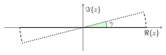
Fig. 1: Schematic representation of the complex contour for the far field integral calculation illustrated in 1D. The full line represents the real domain $\Omega$, the dotted and dashed lines represent the subareas $Z_{1}=\{\bm{x}e^{i\gamma}:x\in\Omega\subset\mathbb{R}\}$ and $Z_{2}=\{be^{i\theta}:b\in\partial\Omega,~{}\theta\in[0,\gamma]\}$ of the complex contour respectively.

3.1 Reformulation to a complex contour

The far field integral (15) can be split into a sum of two contributions: $F(\bm{\alpha})=I_{1}+I_{2}$, with

$$I_{1} =k_{0}^{2}\int_{\Omega}e^{-ik_{0}\bm{x}\cdot\bm{\alpha}}\chi(\bm{x})u_{in}(\bm{x})d\bm{x},$$ (17)

$$I_{2} =k_{0}^{2}\int_{\Omega}e^{-ik_{0}\bm{x}\cdot\bm{\alpha}}\chi(\bm{x})u^{N}(\bm{x})d\bm{x}.$$ (18)

Calculation of the integral $I_{1}$ is generally easy, since it only requires the expression for the incoming wave which is known analytically. The second integral however requires the solution of the Helmholtz equation on the domain $\Omega$ (numerical box), which is notoriously hard to obtain using iterative methods. Hence, the calculation of the scattered wave $u^{N}$ forms a major bottleneck in the traditional calculation of the far field map.

However, if both $u$ and $\chi$ are analytical functions the integral can be calculated over a complex contour rather than the real domain as follows. Let us define a complex contour along the rotated real domain $Z_{1}=\{\bm{z}\in\mathbb{C}\,|\,\bm{z}=\bm{x}e^{i\gamma}:\bm{x}\in\Omega\}$, where $\gamma$ is a fixed rotation angle, followed by the curved segment $Z_{2}=\{\bm{z}\in\mathbb{C}\,|\,\bm{z}=\bm{b}e^{i\theta}:\bm{b}\in\partial\Omega,~{}0\leq\theta\leq\gamma\}$, as presented schematically on Figure 1 for a 1D domain. The extension of the domain to multiple dimensions is straightforward, see [4, 25, 34]. Integral $I_{2}$ can then be written as

$$I_{2}=k_{0}^{2}\int_{Z_{1}}e^{-ik_{0}\bm{z}\cdot\bm{\alpha}}\chi(\bm{z})u^{N}(\bm{z})d\bm{z}+k_{0}^{2}\int_{Z_{2}}e^{-ik_{0}\bm{z}\cdot\bm{\alpha}}\chi(\bm{z})u^{N}(\bm{z})d\bm{z}.$$ (19)

The second term in the above expression vanishes, since the function $\chi$ is per definition zero everywhere outside the object of interest $O$, thus notably in all points $\bm{z}\in Z_{2}$. Hence, we obtain

$$I_{2}=k_{0}^{2}\int_{Z_{1}}e^{-ik_{0}\bm{z}\cdot\bm{\alpha}}\chi(\bm{z})u^{N}(\bm{z})d\bm{z}=k_{0}^{2}\int_{\Omega}e^{-ik_{0}e^{i\gamma}\bm{x}\cdot\bm{\alpha}}\chi(\bm{x}e^{i\gamma})u^{N}(\bm{x}e^{i\gamma})e^{i\gamma}\,d\bm{x}.$$ (20)

Note that for $0<\gamma<\pi/2$ the exponential of $\bm{x}e^{i\gamma}$ is increasing in all directions. At the same time the scattered wave solution $u^{N}$, which consists of outgoing waves on the complex domain $Z_{1}$, is decaying in all directions. Additionally, the function $\chi$ is presumed to have a bounded support (or vanish at infinity, see Section 2.3), making the above integral computable on a limited numerical domain.

Formulation (20) of the integral $I_{2}$ is theoretically equivalent to the original formulation (18), since both formulations result in the same value for the integral. However, the reformulation to the complex contour provides a significant advantage from a computational point of view. Indeed, (20) indicates that the far field map can (at least partially) be computed over the full complex contour $Z_{1}$, that is, a rotation of the original real-valued domain $\Omega$ over an angle $\gamma$ in all spatial dimensions. Contrary to the original integral formulation (18), which required the scattered wave $u^{N}$ evaluated along the real domain, formulation (20) now requires the scattered wave $u^{N}$ along the complex contour. Consequently, for our new approach, the first step in the far field map calculation consists of solving the Helmholtz equation (5) on a complex contour, i.e.

$$\left(-\Delta-k^{2}(\bm{z})\right)u(\bm{z})=k_{0}^{2}\chi(\bm{z})u_{in}(\bm{z}),\qquad\bm{z}\in Z_{1},$$ (21)

which is known to be much easier to solve than the original real-valued Helmholtz equation. Classical multigrid methods allow for a fast solution of damped Helmholtz systems, see [17].

The above integral reformulation (20) implies no restrictions on the value of the rotation angle. Indeed, the rotation angle $\gamma$ can in principle be chosen anywhere in the interval $[0,\pi/2]$, as the equivalence between formulation (18) and (20) theoretically holds for any angle $\gamma$. However, it will be shown in Section 3.3 that in practice, a lower bound on the rotation angle $\gamma$ is implied by the numerical computation of the scattered wave $u^{N}$ in the first step of the far field map computation. Note that, on the other hand, the principal incentive for not choosing $\gamma$ excessively large is the stability of the numerical integration scheme. When the angle $\gamma$ is very large, the scattered wave is heavily damped in all regions remote from the origin, and the integration scheme typically requires additional evaluation points near the origin, cf. [22].

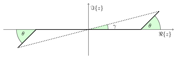
Fig. 2: Schematic representation of a real grid with absorbing boundaries with ECS angle $\theta$ (solid line) vs. a full complex grid with rotation angle $\gamma$ (dotted line), illustrated in 1D. The solid line is the classical domain for the real-valued solution $u^{N}(\bm{x})$ to (5), whereas the dotted line represents the domain $Z_{1}$ for the complex-valued solution $u^{N}(\bm{z})$.

3.2 Solving the Helmholtz equation on a complex domain

We now show that the formulation of the Helmholtz problem on a complex rotated domain like $Z_{1}$ is very similar to a complex shifted Laplacian system [17]. Indeed, both formulations can be shown to be generally equivalent, and hence are equally efficiently solvable. Consider a Helmholtz problem on a complex rotated grid of the form (21)

$$\left(-\Delta-k^{2}(\bm{z})\right)u(\bm{z})=b(\bm{z}),\qquad\bm{z}\in Z_{1}.$$ (22)

This equation is discretized using finite differences on a $d$-dimensional Cartesian grid with a complex valued grid distance $\tilde{h}=e^{i\gamma}h$ (with $h\in\mathbb{R}$) in every spatial dimension, yielding a linear system of the form

$$-\left(\frac{1}{e^{i\varphi}h^{2}}L+k^{2}\right)u_{h}=b_{h},$$ (23)

with $\varphi=2\gamma$ and where $L$ is the matrix operator expressing the stencil structure of the Laplacian. For example, discretization of the 2D Laplacian using second order finite differences yields $L=\text{kron}(I,\text{diag}(-1,2,-1)+\text{kron}(\text{diag}(-1,2,-1),I)$, where the size of $L$ intrinsically depends on $h$. Rewriting the rotation as $\exp{(i\varphi)}=(\alpha+i\beta)$, and multiplying both sides in (23) by $(\alpha+i\beta)$, we obtain the equivalent system

$$-\left(\frac{1}{h^{2}}L+(\alpha+i\beta)k^{2}\right)u_{h}=(\alpha+\beta i)\,b_{h}.$$ (24)

The left-hand side matrix operator of this equation is a discretization of the complex shifted Helmholtz operator $-\Delta-(\alpha+\beta i)k^{2}$. We momentarily assume $k$ to be real-valued; an analogous argument can be used for complex-valued wavenumbers under proper conditions. Hence, (24) is the discrete representation of a CSL system, which is known to be solvable using multigrid given a sufficiently large complex shift $\beta$ [16]. Note that in the CSL literature, the real part of the shift factor is commonly chosen as $\alpha=1$, yielding a shift of the form $-(1+i\beta)k^{2}$ [17]. We expound on the relation between the complex shift $\beta$ and the rotation angle $\gamma$ in Section 3.3.

The scheme given by (23) is known as Complex Stretched Grid (CSG), and was shown in [34] to hold very similar properties with respect to multigrid convergence compared to the complex shifted Laplacian system. Moreover, it is shown above that the CSL and CSG schemes are generally equivalent, and thus can be solved equally efficiently using a multigrid method.

3.3 On the rotation angle

The choice of a sufficiently large complex shift parameter $\beta$ is vital to the stability of the multigrid solution method for problem (24), or equivalently (23). When the shift parameter is chosen below a certain minimal value denoted as $\beta_{min}$, the multigrid scheme tends to be unstable and convergence will break down. A typical rule of thumb for the choice of the complex shift suggested in the CSL literature is $\beta\geq 0.5$ [14, 17]. Note that the lower limit $\beta_{min}=0.5$ is based on a multigrid V-cycle with standard weighted Jacobi or Gauss-Seidel smoothing. However, more advanced iterative techniques like ILU [40] or GMRES [11] may alternatively be used as a smoother substitute in the multigrid solver.

The requirement of a minimal shift for multigrid stability on the CSL problem can be directly translated into a minimal rotation angle $\gamma$ for the complex scaled system. Writing the complex shift in polar notation

$$(1+i\beta)=\rho\exp(i\varphi),$$ (25)

where $\rho=\sqrt{1+\beta^{2}}$ and $\varphi=\arctan\beta$, one readily obtains

$$\tilde{h}=\sqrt{1+i\beta}\,h=\sqrt{\rho}\exp(i\varphi/2)\,h.$$ (26)

Denoting the minimal value of the complex shift by $\beta_{min}$, the rotation angle $\gamma=\varphi/2$ must satisfy

$$\gamma\geq\frac{\arctan(\beta_{min})}{2}.$$ (27)

For the rule of thumb $\beta_{min}=0.5$ stated above, this implies that $\gamma\geq 0.23\approx 13^{\circ}$. Note that when substituting the standard stationary multigrid relaxation scheme ($\omega$-Jacobi, Gauss-Seidel) by a more robust iterative scheme like GMRES(m) (with $m=2$ or $3$), the rotation angle $\gamma$ is typically chosen at around $10^{\circ}$, resulting in a stable multigrid scheme.

In this paper we have chosen to link the grid rotation angle $\gamma$ to the standard ECS absorbing layer angle $\theta$, as shown in Figure 2. This is in no way imperious for the functionality of the method, but it appears quite naturally from the fact that both angles perturb (part of) the grid into the complex plane. Supposing the ECS boundary layer measures one quarter of the length of the entire real domain in every spatial dimension, which is a common choice, we readily derive the following relation between the rotation angle $\gamma$ and the ECS angle $\theta$:

$$\gamma=\arctan\left(\frac{\sin\theta}{2+\cos\theta}\right).$$ (28)

Table 1 shows some standard values of the ECS angle $\theta$ and corresponding $\gamma$ values according to (28). Following (27), we note that for a multigrid scheme with $\omega$-Jacobi or Gauss-Seidel smoothing to be stable, $\theta$ should be chosen no smaller than $\pi/4$. Using the more efficient GMRES(3) method as a smoother replacement, an ECS angle around $\theta=\pi/6$ suffices to guarantee stable multigrid convergence.

On the other hand, taking $\gamma$ too large has some drawbacks which are reflected in the accuracy of the numerical scheme for the calculation of the far-field integral. For $\gamma>0$, the solution $u^{N}(\bm{z})$ is an exponentially decaying function towards the boundary. At the same time, the function $e^{-ik_{0}\bm{z}\cdot\mathbf{\alpha}}$ is exponentially growing towards the boundary. Their product, which appears in the integral, remains bounded. However, when $\gamma$ is chosen to be very large, the difference in magnitude between the two integrand factors can affect the accuracy of the numerical integral. Indeed, when multiplying two floating point numbers, one being extremely small and the other extremely large, and each is represented up to machine precision, the numerical error on this multiplication can be very large. These considerations somewhat limits the choice of the rotation angle for the complex contour.

$\theta$ (rad.)	$\pi/8$	$\pi/7$	$\pi/6$	$\pi/5$	$\pi/4$	$\pi/3$
$\gamma$ (deg.)	$7.5^{\circ}$	$8.5^{\circ}$	$9.9^{\circ}$	$11.8^{\circ}$	$14.6^{\circ}$	$19.1^{\circ}$

Table 1: ECS angle $\theta$ and corresponding rotation angle $\gamma$ for the full complex grid. Values based on (28).

4 Numerical results for 2D and 3D Helmholtz problems

In this section, we validate the theoretical result presented above by a number of numerical experiments in both two and three spatial dimensions. We make use of the known efficiency of multigrid in solving damped Helmholtz equations to compute the solutions to the Helmholtz systems required in the complex valued far field integral.

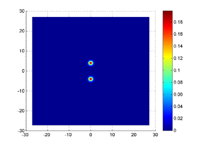
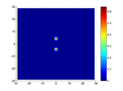
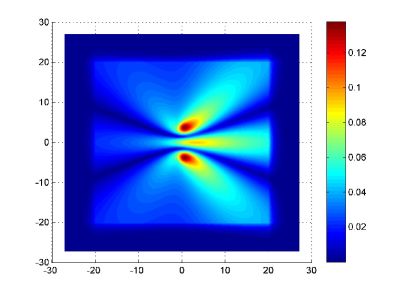
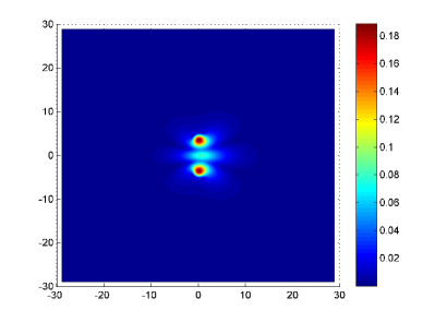
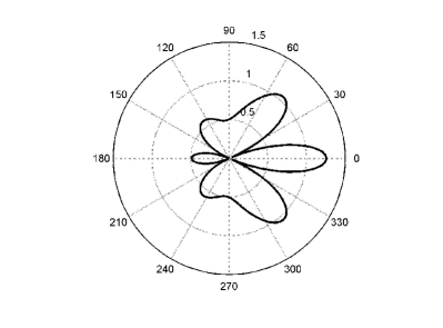
Fig. 3: Comparison between the classical real-valued far field map calculation method (left) and the new complex-valued approach (right). Top: 2D object of interest $|\chi|$ given by (29). Mid: solutions to the Helmholtz problem (5) (in modulus) on a $n_{x}\times n_{y}=256\times 256$ grid. Left: real-valued problem with double ECS contour with $\theta=\pi/4$ solved using LU factorization. Right: complex-valued problem solved using a series of multigrid V-cycles with $\omega$-Jacobi smoother on the corresponding full complex contour with $\gamma=14.6^{\circ}$ up to a residual reduction tolerance of 1e-6. Bottom: resulting 2D Far field map $F(\alpha)$ for both approaches, calculated following (15). Normalized errors with respect to a $n_{x}\times n_{y}=1024\times 1024$ grid benchmark Far field map solution $F_{ex}(\alpha)$: $\|F_{re}-F_{ex}\|_{2}/\|F_{ex}\|_{2}=$ 9.37e-5 (left), $\|F_{co}-F_{ex}\|_{2}/\|F_{ex}\|_{2}=$ 1.39e-4 (right), $\|F_{re}-F_{co}\|_{2}/\|F_{ex}\|_{2}=$ 1.77e-4.

The model problem used throughout this section is a Helmholtz equation of the form (5) with $k^{2}(\bm{x})=k_{0}^{2}(1+\chi(\bm{x}))$. The equation is discretized on a $n^{d}$-point uniform Cartesian mesh covering a square numerical domain $\Omega=[-20,20]^{d}$ using second order finite differences. Note that the use of a different discretization scheme would not fundamentally affect the results presented in this work. In the 2D case the space-dependent wavenumber is defined as

$$k_{0}^{2}\,\chi(x,y)=-1/5\left(e^{-(x^{2}+(y-4)^{2})}+e^{-(x^{2}+(y+4)^{2})}\right),\quad(x,y)\in[-20,20]^{2},$$ (29)

i.e. the object of interest takes the form of two circular point-like objects with mass concentrated at the Cartesian coordinates $(0,-4)$ and $(0,4)$, see Figure 3 (top panel). For the 3D model problem, the following straightforward extension of the object is used

$$k_{0}^{2}\,\chi(x,y,z)=-1/5\left(e^{-(x^{2}+(y-4)^{2}+z^{2})}+e^{-(x^{2}+(y+4)^{2}+z^{2})}\right),\quad(x,y,z)\in[-20,20]^{3},$$ (30)

representing two spherical point-like objects in 3D space, see Figure 4 (left panel). The incoming wave scattering at the given object is defined by

$$u_{in}(\bm{x})=e^{ik_{0}\bm{\eta}\cdot\bm{x}},\quad\bm{x}\in\Omega,$$ (31)

where $\bm{\eta}$ is the unit vector in the $x$-direction.

	$n_{x}\times n_{y}\times n_{z}$	$16^{3}$	$32^{3}$	$64^{3}$	$128^{3}$	$256^{3}$
$k_{0}$	1/4	10 (10)	9 (59)	9 (560)	9 (4456)	9 (35165)
		0.24	0.20	0.21	0.20	0.20
	1/2	12 (12)	10 (63)	10 (611)	10 (4937)	9 (35405)
		0.31	0.24	0.22	0.23	0.21
	1	7 (8)	13 (83)	11 (691)	10 (4899)	10 (38975)
		0.13	0.32	0.27	0.24	0.24
	2	2 (4)	8 (54)	13 (809)	11 (5418)	10 (38051)
		0.01	0.14	0.33	0.27	0.24
	4	1 (3)	2 (17)	7 (457)	13 (6337)	11 (41848)
		0.01	0.01	0.12	0.33	0.26

Table 2: 3D Helmholtz problem (5) solved on a full complex grid with $\theta=\pi/6$ $(\gamma=9.9^{\circ})$ using a series of multigrid V(1,1)-cycles with GMRES(3) smoother up to residual reduction tolerance 1e-6. Displayed are the number of V-cycle iterations, number of work units and average convergence factor for various wavenumbers $k_{0}$ and different discretizations. 1 WU is calibrated as the cost of 1 V(1,1)-cycle on the $16^{3}$-points grid $k_{0}=1/4$ problem. Discretizations respecting the $k_{0}h<0.625$ criterion for a minimum of 10 grid points per wavelength are indicated by a bold typesetting.

Figure 3 validates the equivalence between the classical real-valued far field map integral from Section 2 and the new complex contour formulation presented in Section 3. The 2D Helmholtz model problem with wavenumber given by (29) and $k_{0}=1$ is solved for $u^{N}$ using respectively a standard LU factorization method on the real domain $\Omega$ with ECS complex boundary layers ($\theta=\pi/4$) along the domain boundary $\partial\Omega$, and a series of multigrid V(1,1)-cycles with $\omega$-Jacobi smoothing on the full complex domain ($\gamma=14.6^{\circ}$) with a residual reduction tolerance of 1e-6. The standard multigrid intergrid operators used in this work are bilinear interpolation and full weighting restriction. The moduli of the wavenumber function $\chi$ (top) and the resulting solution $u^{N}$ (mid) are shown on Figure 3 for both methods. Note how the solution $u^{N}$ on the full complex contour (right) is indeed heavily damped compared to the solution on the real domain (left). Consequently, using the numerical solution $u^{N}$, the 2D far field map integral (15) can be calculated using any numerical integration scheme over the real or complex domain respectively. The resulting far field map $F(\bm{\alpha})$ is shown as a function of the angle $\alpha$ on Figure 3 (bottom). One observes that the mapping is indeed identical when calculated over the real-valued (left) and complex-valued (right) domain, conform with the theoretical results. The normalized difference between both far field computations does not exceed 0.177% (in norm), which is effectively of the same order of magnitude as the normalized error. However, the computational cost of the real-domain method for calculation of the far field map is reduced significantly by the ability to apply multigrid to the equivalent complex scaled problem.

	$n_{x}\times n_{y}\times n_{z}$	$16^{3}$	$32^{3}$	$64^{3}$	$128^{3}$	$256^{3}$
$k_{0}$	1/4	8 (11)	6 (52)	5 (384)	5 (3190)	5 (25241)
		1.93e-9	1.77e-9	2.46e-9	2.68e-9	3.00e-9
	1/2	9 (12)	8 (68)	6 (452)	6 (3392)	6 (30215)
		1.27e-8	1.87e-9	3.37e-9	1.30e-9	1.25e-9
	1	5 (8)	9 (68)	8 (572)	7 (4013)	6 (30747)
		1.33e-8	1.51e-8	4.07e-9	1.76e-9	3.66e-9
	2	1 (5)	5 (43)	9 (600)	8 (4456)	7 (36367)
		5.99e-13	1.18e-8	1.91e-8	5.28e-9	2.67e-9
	4	1 (4)	1 (18)	5 (357)	9 (5038)	8 (39038)
		8.90e-20	2.86e-13	5.19e-9	1.97e-8	4.65e-9

Table 3: 3D Helmholtz problem (5) solved on a full complex grid with $\theta=\pi/6$ $(\gamma=9.9^{\circ})$ using an FMG cycle with GMRES(3) smoother up to residual reduction tolerance of 1e-6. Displayed are the number of V-cycle iterations on the designated finest grid, number of work units and resulting residual norm for various wavenumbers $k_{0}$ and different discretizations. 1 WU is calibrated as the cost of 1 V(1,1)-cycle on the $16^{3}$-points grid $k_{0}=1/4$ problem. Discretizations respecting the $k_{0}h<0.625$ criterion for a minimum of 10 grid points per wavelength indicated by a bold typesetting.

In Table 2 convergence results are shown for the solution of the 3D scattered wave equation (5) using a series of multigrid V(1,1)-cycles on various grid sizes. Note that the multigrid method scales perfectly as a function of the number of grid points, as doubling the number of grid points in every spatial dimension does not increase the number of V-cycles required to reach a fixed residual tolerance of 1e-6. This is a standard result from multigrid theory. Additionally and more importantly, remarkable $k$-scalability is measured for the multigrid solution method on the complex contour. Indeed, the multigrid convergence factor (and thus the corresponding work unit load required to solve the problem up to a given tolerance) is almost fully independent of the wavenumber $k_{0}$, as can be observed from the table. From a physical-numerical point of view it is only meaningful to consider discretizations satisfying the $k_{0}h<0.625$ criterion for a minimum of 10 grid points per wavelength, cf. [4], for which the corresponding values are designated in Table 2 by a bold typesetting.

Ultimately, the computed scattered wave solution on the 3D complex domain can be used to calculate the far field integral (15). The resulting 3D far field mapping for the model problem with $k_{0}=1$ is shown in Figure 4. The left hand side panel shows an isosurface visualization of the 3D object of interest $\chi(\bm{x})$ given by (30). On the right panel a spherical projection of the resulting 3D far field mapping is shown. The color hue indicates the value of the far field amplitude in each outgoing direction.

Note that the calculation of the scattered wave solution can be optimized even further by considering the Full Multigrid (FMG) scheme. This is a nested iteration of standard V-cycles, where on each level a series of V(1,1)-cycles is used to approximately solve the error equation and supply a corrected initial guess for a finer level by interpolating the corresponding coarse grid solution.

Table 3 shows convergence results for the solution of the 3D scattered wave equation (5) using an FMG scheme. The setting is comparable to that of Table 2. A residual reduction tolerance of $10^{-6}$ is imposed for each wavenumber and at every level of the FMG cycle, yielding a fine $n_{x}\times n_{y}\times n_{z}=256^{3}$ grid residual of order of magnitude $10^{-9}$. Note that the number of V-cycles performed on each level in the FMG cycle is decaying as a function of the growing grid size due to the increasingly accurate initial guess, resulting in a relatively small number of V-cycles (five to nine) to be performed on the finest level. Consequently, the number of work units (and thus the computational time) required to reach the designated residual reduction tolerance is significantly lower than the work unit load of the pure V-cycle scheme displayed in Table 2.

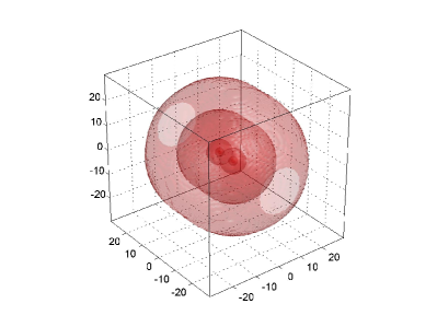
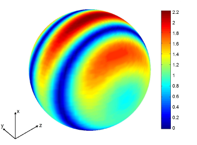
Fig. 4: Left: 3D object of interest $|\chi(\bm{x})|$ given by (30). Shown are the $|\chi(\bm{x})|=c$ isosurfaces for $c=$ 1e-1, 1e-2, 1e-10, 1e-100 and 1e-300. Right: 3D Far field map, resulting from Helmholtz problem (5) with $k_{0}=1$ solved on a $n_{x}\times n_{y}\times n_{z}=64\times 64\times 64$ full complex grid with $\theta=\pi/6$ ($\gamma\approx 9.9^{\circ}$) using a series of multigrid V-cycles with GMRES(3) smoother up to residual reduction tolerance 1e-6.

$n_{x}\times n_{y}\times n_{z}$	$16^{3}$	$32^{3}$	$64^{3}$	$128^{3}$	$256^{3}$
CPU time	0.20 s.	0.78 s.	6.24 s.	53.3 s.	462 s.
$\|r\|_{2}$	3.3e-5	7.9e-5	2.7e-5	1.1e-5	4.6e-6

Table 4: 3D Helmholtz problem (5) with wavenumber $k_{0}=1$ solved on a full complex grid with $\theta=\pi/6$ $(\gamma=9.9^{\circ})$ using one FMG-cycle with GMRES(3) smoother. Displayed are the CPU time (in s.) and the resulting residual norm for various discretizations. System specifications: Intel^® Core${}^{\text{\tiny TM}}$ i7-2720QM 2.20GHz CPU, 6MB Cache, 8GB RAM.

Timing and residual results from a standard FMG sweep performing only one V(1,1)-cycle on each level on the 3D Helmholtz scattering problem with a moderate wavenumber $k_{0}=1$ are shown in Table 4 for different discretizations. Note that timings were generated using a basic non-parallelized Matlab code, using only a single thread on a simple midrange personal computer (system specifications: see caption Table 4) and taking less than 8 minutes to solve a 3D Helmholtz problem with $256$ grid points in every spatial dimension.

5 Application to Schrödinger equations

This section illustrates the application of the proposed complex contour method to Schrödinger equations that are used to describe quantum mechanical scattering problems. The $d$-dimensional time-independent Schrödinger equation for a system with unit mass is given by

$$\left(-\frac{1}{2}\Delta+V(\mathbf{x})-E\right)\psi(\mathbf{x})=\phi(\mathbf{x}),\quad\text{for}~{}\textbf{x}\in\mathbb{R}^{d},$$ (32)

where $\Delta$ is the $d$-dimensional Laplacian, $V(\mathbf{x})$ is a scalar potential, $\psi$ is the wave function and $\phi$ is the right-hand side, which is often related to the ground state of the system. Depending on the total energy $E\in\mathbb{R}$, the above system allows for scattering solutions, in which case the equation can be reformulated as a Helmholtz equation of the form

$$(-\Delta-k^{2}(\mathbf{x}))\,\psi(\mathbf{x})=2\phi(\mathbf{x}),\quad\text{for}~{}\textbf{x}\in\mathbb{R}^{d},$$ (33)

where the spatially dependent wavenumber $k(\mathbf{x})$ is defined by $k^{2}(\mathbf{x})=2(E-V(\mathbf{x}))$. The experimental observations from this type of quantum mechanical systems are typically far field maps of the solution [43]. Indeed, in an experimental setup, detectors are commonly placed at large distances from the object compared to the size of the system. These detectors consequently measure the probability of particles escaping from the system in certain directions. In many quantum mechanical systems the potential $V(\mathbf{x})$ is an analytical function, which suggests analyticity of the wavenumber $k(\mathbf{x})$ in the above Helmholtz equation. Additionally, the potential is often a decaying function. Hence, for these types of problems, the wavenumber naturally satisfies all conditions for the use of the proposed complex contour method to efficiently calculate the corresponding far field map.

In the paragraphs below, we first discuss a 2D model problem where single and double ionization occur, corresponding to waves describing respectively a single particle or two particles escaping from the quantum mechanical system. The first leads to very localized evanescent waves that propagate along the boundaries of the computational domain, while the latter gives rise to waves traversing the full domain. The corresponding 2D Schrödinger problem will be solved on a discretized numerical domain for a range of energies $E$ below and above the double ionization energy threshold. For each energy, we extract the single and double ionization cross sections, which correspond to probabilities of particles escaping from the system, with the help of an integral of the Green’s function over the numerical box. The cross sections are calculated using both a traditional method, where the Helmholtz equation is solved on a standard ECS-bounded grid [26], and the new complex contour method, introduced in Section 3.

The main purpose of the calculations in Sections 5.1 to 5.4 is to validate the complex contour method when applied to Schrödinger’s equation. In Section 5.5 the multigrid performance for solving the 2D complex-valued scattered wave system is benchmarked. Note, however, that these 2D problems essentially do not require a multigrid solver, since a direct sparse solver performs well for these relatively small-size problems. In Section 5.6 we illustrate the convergence of a multigrid solver on a 3D Schrödinger equation, with energies that allow for triple ionization as well as double and single ionization. The previous attempts to solve these problems with the help of the complex shifted Laplacian as a preconditioner to a general Krylov method showed a notable deterioration in the convergence behavior in function of the total energy $E$ [34]. It will be shown that the new complex contour method, which allows to use multigrid as a solver, performs well for these problems.

Although the benchmark problems considered in this section mainly use model potentials, we believe that the calculations presented below are an important step towards the application of the method on realistic quantum mechanical systems.

5.1 Cross sections of the 2D Schrödinger problem

Our primary aim is to validate the applicability of the new complex contour method on the 2D Schrödinger equation describing a quantum mechanical scattering problem. This problem originates from the expansion of a 6D scattering problem in spherical harmonics, see [2, 43], in which each particle is expressed in terms of its spherical coordinates, resulting in a coupled system of 2D equations. Note that the differential operators only appear on the diagonal blocks of the system. These diagonal blocks then form the two-dimensional Schrödinger equation

$$\left(-\frac{1}{2}\Delta+V_{1}(x)+V_{2}(y)+V_{12}(x,y)-E\right)u(x,y)=\phi(x,y),\quad x,y\geq 0,$$ (34)

with boundary conditions

$$\begin{cases}u(x,0)=0\quad\text{for}\quad x\geq 0\\ u(0,y)=0\quad\text{for}\quad y\geq 0\\ \text{outgoing}\quad\text{for}\quad x\rightarrow\infty\quad\text{or}\quad y\rightarrow\infty,\end{cases}$$ (35)

where $\Delta$ represents the 2D Laplacian, $V_{1}(x)$ and $V_{2}(y)$ are the one-body potentials, $V_{12}(x,y)$ is a two-body potential and $E$ is the total energy of the system. Since the arguments $x$ and $y$ are in fact radial coordinates in the partial wave expansion, homogeneous Dirichlet boundary conditions are implied at the $x=0$ and $y=0$ boundaries. The potentials $V_{1}$, $V_{2}$ and $V_{12}$ are generally analytical functions that decay as the radial coordinates $x$ and $y$ become large.

Depending on the strength of the one-body potentials $V_{1}$ and $V_{2}$, the problem allows for so-called single ionization waves, which are localized evanescent waves that propagate along the edges of the domain. We refer the reader to Sections 5.2 and 5.3 for a more detailed physical clarification. In the following, we expound on the situation with a strong attractive potential $V_{1}$ in the $x$-direction; the case with a strong $V_{2}$ potential is completely analogous. If the attraction of $V_{1}$ is strong enough, there exists a one-dimensional eigenstate $\phi_{n}(x)$ for every negative eigenvalue $\lambda_{n}<0$, characterized by a one-dimensional Helmholtz equation

$$\left(-\frac{1}{2}\frac{d^{2}}{dx^{2}}+V_{1}(x)\right)\phi_{n}(x)=\lambda_{n}\,\phi_{n}(x),\quad\text{for}~{}x\geq 0.$$ (36)

Note that $\phi_{n}(0)=0$ and $\phi_{n}(x\rightarrow\infty)=0$.

The far field maps of this system are then again Green’s integrals over the solution, see [26]. Indeed, the single ionization amplitude $s_{n}(E)$, which represents the total number of single ionized particles, is given by

$$s_{n}(E)=\int_{\Omega}\phi_{k_{n}}(x)\phi_{n}(y)\left[\phi(x,y)-V_{12}(x,y)u(x,y)\right]\,dx\,dy,$$ (37)

where $k_{n}=\sqrt{2(E-\lambda_{n})}$, $\phi_{n}$ is a one-body eigenstate, i.e.  a solution of equation (36) with a corresponding eigenvalue $\lambda_{n}$, and the function $\phi_{k_{n}}$ is a regular, normalized solution of the homogeneous Helmholtz equation

$$\left(-\frac{1}{2}\frac{d^{2}}{dx^{2}}+V_{1}(x)-\frac{1}{2}k^{2}\right)\phi_{k}=0,$$ (38)

where $k=k_{n}$ and $\phi_{k_{n}}$ normalized with $1/\sqrt{k_{n}}$.

Similarly, the double ionization cross section $f(k_{1},k_{2})$, which measures the total number of double ionized particles, is defined by the integral

$$f(k_{1},k_{2})=\int_{\Omega}\phi_{k_{1}}(x)\phi_{k_{2}}(y)\left(\phi(x,y)-V_{12}(x,y)u(x,y)\right)\,dx\,dy,\quad x,y\geq 0,$$ (39)

where both $\phi_{k_{1}}(x)$ and $\phi_{k_{2}}(y)$ are solutions to (38), with $k_{1}=\sqrt{2E}\sin(\alpha)$ and $k_{2}=\sqrt{2E}\cos(\alpha)$, respectively, and $\alpha\in[0,\pi/2]$ such that $k_{1}^{2}+k_{2}^{2}=2E$. The total double ionization cross section is defined as the integral

$$\sigma_{tot}(E)=\int_{0}^{E}\sigma(\sqrt{2\epsilon},\sqrt{2(E-\epsilon)})\,d\epsilon,$$ (40)

where

$$\sigma(k_{1},k_{2})=\frac{8\pi^{2}}{k_{0}^{2}}\frac{1}{k_{1}k_{2}}|f(k_{1},k_{2})|^{2}.$$ (41)

The above integral expressions are obtained through a reorganization similar to the one performed in Section 2, see (6)-(7). For example, to calculate the single ionization cross section, equation (34) is reorganized as

$$\left(-\frac{1}{2}\Delta+V_{1}(x)-E\right)u(x,y)=\phi(x,y)-(V_{2}(y)+V_{12}(x,y))\,u(x,y),\quad x,y\geq 0.$$ (42)

Since the left hand side is separable, the corresponding Green’s function allows us to write

$$u(x,y)=\int_{\Omega}G(x,y|x^{\prime},y^{\prime})\left(\phi(x^{\prime},y^{\prime})-(V_{2}(y^{\prime})+V_{12}(x^{\prime},y^{\prime}))\,u^{N}(x^{\prime},y^{\prime})\right)\,dx^{\prime}\,dy^{\prime}.$$ (43)

Using the asymptotic form of the Green’s function, the above ultimately results in integral formulation (37). The double ionization integral expression (39) can be derived in a similar way.

5.2 Spectral properties of the 2D Schrödinger problem

To obtain insight in the multigrid convergence for the two-dimensional Schrödinger problem, we briefly discuss the spectral properties of the discretized Schrödinger operator. The discretized 2D Hamiltonian $H^{2d}$ corresponding to equation (34) can be written as a sum of two Kronecker products and a two-body potential, i.e.

$$H^{\text{2d}}=H^{\text{1d}}\otimes I+I\otimes H^{\text{1d}}+V_{12}(x,y),$$ (44)

where $H^{\text{1d}}=-1/2\Delta+V_{i}$ $(i=1,2)$ is the one-dimensional Hamiltonian, discretized using finite differences. When the two-body potential $V_{12}(x,y)$ is weak relative to the one-body potentials, the eigenvalues of the 2D Hamiltonian can be approximated by

$$\lambda^{\text{2d}}\approx\lambda_{i}^{\text{1d}}+\lambda_{j}^{\text{1d}},\qquad 1\leq i,j,\leq n.$$ (45)

Hence, to form a better understanding of the spectral properties of $H^{\text{2d}}$, let us first consider the eigenvalues of $H^{1d}$. After discretization using second order finite differences, the one-dimensional Hamiltonian can be written as a tridiagonal matrix, where the stencil

$$\frac{1}{h^{2}}\left[\begin{matrix}-1&2&-1\end{matrix}\right]$$ (46)

approximates the second derivatives, and the potential is a diagonal matrix evaluated in the grid points. The spectrum of $H^{\text{1d}}$ closely resembles the spectrum of the Laplacian $(-1/2)\Delta$, however the presence of the potential modifies the smallest eigenvalues. The resulting spectrum is shown on the top left panel of Figure 5, which presents a close-up of the eigenvalues near the origin. A single negative eigenvalue $\lambda_{0}^{1d}=-1.0215$ can be observed, which is due to the attractive potential. The remaining spectrum consists of a series of positive eigenvalues located along the positive real axis. The top right panel of Figure 5 shows the eigenvalues of $H^{1d}$, discretized along a complex-valued contour, i.e. the real grid rotated into the complex plane by $\gamma$. The grid distance used is now $\tilde{h}=he^{i\gamma}$, which results in the following stencil for the second derivative

$$e^{-2i\gamma}\frac{1}{h^{2}}\left[\begin{matrix}-1&2&-1\end{matrix}\right].$$ (47)

This implies that the spectrum of the Laplacian is rotated down into the complex plane by an angle $2\gamma$. Figure 5 shows that most of the eigenvalues of $H^{\text{1d}}$ are rotated downwards over $2\gamma$, with the exception of the bound state eigenvalue $\lambda_{0}^{1d}$, which remains on the negative real axis. The changes of spectrum as a result of a rotation are well known in the physics literature, see for example [29].

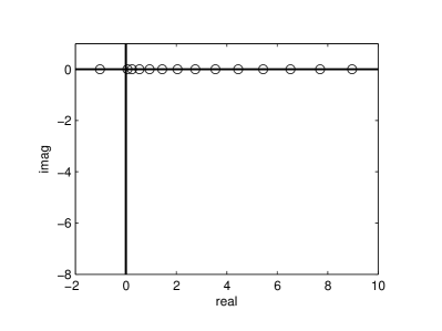
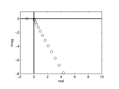
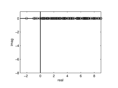
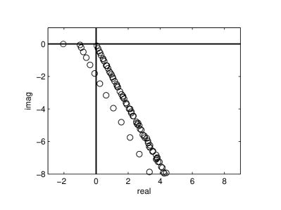
Fig. 5: Spectrum (close-up) of the discretized 1D (top) and 2D (bottom) Hamiltonian (45), i.e. with $E=0$. Left: spectrum corresponding to the standard discretization with real-valued grid distance $h$. Right: spectrum for a complex contour discretization with complex-valued grid distance $\tilde{h}=e^{-i\gamma}h$, where $\gamma=\pi/6$. The complex spectrum is rotated down into the complex plane over $2\gamma=\pi/3$, cf. [34].

We consequently turn to the two-dimensional problem setting, where the eigenvalues of the Hamiltonian $H^{\text{2d}}$ are approximately sums of the one-dimensional operator eigenvalues $H^{\text{1d}}\otimes I+I\otimes H^{\text{1d}}$. The resulting eigenvalues are shown on the bottom two panels of Figure 5. Again, the eigenvalues of the 2D Hamiltonian are rotated down in the complex plane when the system is discretized along a complex-valued contour. In 2D, an isolated eigenvalue appears around $\lambda_{0}^{1d}+\lambda_{0}^{1d}=-2.043$, and two series of eigenvalues emerge from the real axis: a first branch of eigenvalues starting at $-1.012$, which originates from the sum of the negative eigenvalue $\lambda_{0}^{1d}$ of the first 1D Hamiltonian combined with all the positive eigenvalues of the second 1D Hamiltonian; and a second series of eigenvalues starting at the origin, originating from the sums of the positive eigenvalues of both one-dimensional Hamiltonians.

5.3 Solution types: single and double ionization

The Schrödinger equation (34) can be written shortly as $(H-E\,I)u=\phi$, where $H=(-1/2)\Delta+V_{1}+V_{2}+V_{12}$ is the Hamiltonian and the scalar $E$ is the total energy of the system. Depending on this energy $E$, the Schrödinger system has different types of solutions. In this section we briefly expound on the physical interpretation of these solution types, using a model problem example. This section may prove less interesting to readers who are primarily interested in the computational aspects of the solution, and as such can be skipped at will.

When the energy $E$ is larger than the smallest (negative) eigenvalue of the Hamiltonian, i.e. $\lambda_{0}<E$, one-body eigenstate solutions to (36) arise. These eigenstates can be combined into separable waves of the form

$$u_{n}(x,y)=\phi_{n}(x)\exp(ik_{n}y),$$ (48)

with $k_{n}=\sqrt{2(E-\lambda_{n})}$, that form a solution to the Schrödinger problem (34) in the region where $x$ is small and $y\rightarrow\infty$. Indeed, when $y$ is large, the potentials $V_{2}$ and $V_{12}$ are negligibly small and the resulting Schrödinger equation becomes separable in variables, where $\phi_{n}(x)$ and $\exp(ik_{n}y)$ are the solutions of the separated operators respectively. An analogous argument holds for the case when $V_{2}$ dominates and $V_{1}$ and $V_{12}$ are negligibly small, yielding evanescent waves of the form

$$u_{n}(x,y)=\phi_{n}(y)\exp(ik_{n}x).$$ (49)

These separable waves are solutions of the Schrödinger system for $x\rightarrow\infty$ and $y$ small, and can be derived similarly to (48).

Single ionization	Double ionization

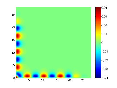
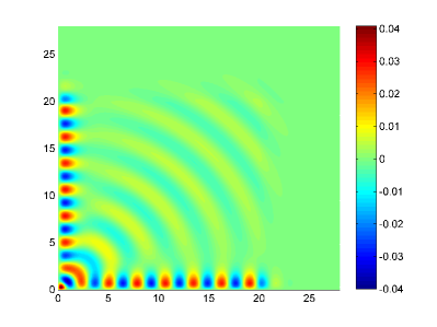
Fig. 6: Scattered wave solutions $u(x,y)$ to model problem (34). Model specifications: see accompanying text. Left: solution for energy $E=-0.5$ where only single ionization occurs. Right: solution for energy $E=1.5$ where both double and single ionization occur. Single ionization waves are localized solely along the edges of the domain (left), while double ionization waves appear both along the edges and in the middle of the domain (right).

Note that we can associate such a separable wave with each eigenstate $\phi_{n}$ of equation (36) that corresponds to a negative eigenvalue of the Hamiltonian. These localized waves are called single ionization waves in the physics literature, since they correspond to a quantum mechanical system in which a single particle is ionized. Single ionization waves are present in the solution as soon as the energy $E$ is above the $\lambda_{0}$ threshold. When there is a second eigenstate with negative energy, say $\phi_{1}$ with $\lambda_{1}$, an additional single ionization wave appears in the problem as soon as $E>\lambda_{1}$. We refer to the specialized literature for a detailed discussion of the ionization process, see [19, 31].

The left panel of Figure 6 shows the solution to (34) for a total energy $E=-0.5$. The model problem under consideration fits equation (34), with a right-hand side given by $\phi(x,y)=\exp(-3(x+y)^{2})$. The one-body potentials are defined by $V_{1}(x)=-4.5\exp(-x^{2})$ and $V_{2}(y)=-4.5\exp(-y^{2})$, yielding an eigenstate of equation (36) with energy $\lambda_{0}=-1.0215$. The two-body potential equals $V_{12}(x,y)={2\exp(-(x+y)^{2})}$. The equation is discretized on a $[0,20]^{2}$ domain using 500 grid points in every spatial dimension. An ECS absorbing layer consisting of an additional 250 grid points damps the outgoing waves along the right and top edges of the domain. Note from Figure 6 how the single ionization eigenstate solutions given by (48)-(49) appear along the edges of the domain.

When the total energy $E>0$, additional asymptotic scattering solutions to the Schrödinger equation appear. If all potentials are asymptotically zero, equation (34) boils down to a Helmholtz equation with wavenumber $k=\sqrt{2E}$ for $x\rightarrow\infty$ and $y\rightarrow\infty$. The resulting waves are known as double ionization waves and physically correspond to the simultaneous ejection of two particles from the quantum mechanical system. In the far field, double ionization waves behave as $e^{i\sqrt{2E}\sqrt{x^{2}+y^{2}}}$, with an angle-dependent prefactor. At the same time, it is still possible to have single ionization for positive energies $E$, since $E>\lambda_{0}$. The right panel of Figure 6 shows the solution for $E=1.5$, clearly displaying the double ionization waves in the middle of the domain and single ionization along the edges, where the two solutions coexist. Additionally, one observes that the single ionization waves oscillate faster in the $x$- or $y$-direction than a free wave with wavenumber $k=\sqrt{2E}$, since $k_{n}\geq k$.

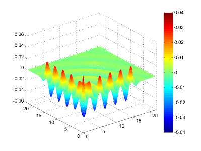
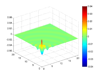
Fig. 7: Scattered wave solutions $u(x,y)$ to model problem (34) for $E=1$. Left: solution on a real grid with ECS absorbing boundary layer $(\theta=\pi/7\approx 25^{\circ})$. Right: solution on a straight complex scaled contour $(\gamma\approx 8.5^{\circ})$, resulting in a damped scattered wave solution.

5.4 Complex contour method for the 2D Schrödinger problem

In physical experiments, the total number of single ionized or double ionized particles is typically observed for a range of energy levels $E$ using advanced detectors. These observations are made far away from the object and effectively measure the far field amplitudes of the solutions. The outcome of this type of experiments can be predicted by calculating the single (37) and double ionization (39) cross sections, using the numerical solution of equation (34), see [26]. Indeed, in order to calculate these cross sections, the numerical solution $u^{N}(x,y)$ to (34) is required, which is generally hard to obtain, especially in higher spatial dimensions. However, since the potentials $V_{1}$, $V_{2}$ and $V_{12}$ are analytical functions, the integrals for single and double ionization can be calculated along a complex contour rather than the classical real domain, in analogy to the discussion in Section 3. Consequently, one requires the scattering solution of equation (34) on a complex contour, which is much easier to compute.

In the following, we calculate the single and double ionization cross sections for a number of energies $E$ between $-1$ and $3$ using both the classical real-valued discretization and the complex contour approach proposed in this paper. The corresponding 2D scattering problems (34) are solved on a numerical domain $\Omega=[0,15]^{2}$ covered by a finite difference grid consisting of 300 grid points in every spatial dimension. Additionally, an ECS absorbing boundary layer starts at $x=15$ and $y=15$, respectively, and implements the outgoing boundary conditions, adding an additional 150 grid points in every spatial dimension. The ECS angle is $\theta=\pi/7\approx 25.7^{\circ}$. For the complex contour method, a complex scaled grid with an overall complex rotation angle $\gamma\approx 8.5^{\circ}$ is used. Solutions $u^{N}(x,y)$ to (34) for a total energy $E=1$ on both the classical real-valued grid and the complex contour are presented on Figure 7. Note how the solution is damped when evaluated along the complex contour.

Fig. 8: Comparison of the single and double ionization total cross sections calculated using the scattered wave solution $u^{N}$ of (34) calculated on (a) a traditional real-valued ECS grid with $\theta=\pi/7$ and (b) a full complex contour with $\gamma=8.5^{\circ}$. The energy range starts at the single ionization threshold $E=-1$, corresponding to a strictly positive cross section. Double ionization occurs for energy levels $E>0$.

Figure 8 shows the rate of single and double ionization as a function of the total energy $E$. The dashed and dotted lines represent the single and double ionization amplitudes calculated using the traditional real-valued method with ECS absorbing boundary conditions [26]. The solid line is the total cross section, i.e.  the sum of single and double ionization, and is calculated using the optical theorem, see [31]. One observes that single ionization occurs starting from $E>-1.0215$. Double ionization only occurs when $E>0$, and comprises only a fraction of the single ionization cross section (cf. Figure 6). Note how the energy of the single ionized bound states rises as the total energy grows, and remains present even when $E>0$. Results obtained using the complex contour approach are indicated by the $\blacktriangle$ and $\bullet$ symbols on Figure 8. In this case, the Schrödinger equation (34) is first solved on a complex contour, yielding a damped solution as shown by Figure 7 (right panel), followed by the calculation of the integrals (37) and (39) along this complex contour. Identical results are obtained by both calculation methods, thus validating the applicability of the complex contour approach on Schrödinger-type problems.

5.5 Multigrid performance on the 2D Schrödinger problem

In this section, we benchmark the performance of multigrid as a solver for the 2D Schrödinger scattering problem on a complex-valued grid. It appears that the multigrid convergence rate critically depends on the value of the total energy $E$. Indeed, Figure 9 shows the convergence rate of a standard multigrid V(1,1)-cycle for the 2D model problem described in the sections above. We observe that the multigrid scheme fails to converge for total energies $E$ between $-1$ and $0$. Note that this corresponds precisely to the energy range where only single ionization occurs. However, for energy levels $E>0$, where both single and double ionization occur, multigrid successfully converges.

The observed convergence behavior can be explained using the spectral properties of the Hamiltonian operator introduced in Section 5.2. The bottom right panel of Figure 5 shows the eigenvalues of $H^{\text{1d}}\otimes I+I\otimes H^{1d}$, which approximate the spectrum of $H^{\text{2d}}$, discretized along a complex contour. Changing the total energy $E$ shifts the spectrum of the linear system $(H^{2d}-E)u=\phi$ to the left or right. For $-1<E<0$ the spectrum shifts to the right, resulting in a spectrum with real-valued eigenvalues both to the left and right of the origin. This indeed implies difficulties for both the smoother and the coarse grid correction scheme. However, when $0<E$, the spectrum shifts to the left, moving all eigenvalues away from zero. This results in a spectrum that is distinctly separated from the origin, corresponding to a problem more amenable to iterative solution.

From figure 9, it might appear to the reader that multigrid is not generally efficient as a Schrödinger solver due to the poor convergence in the $-1<E<0$ region. However, it is important to note that multigrid is performant in the region of physical interest. Indeed, the double ionization problem requires a full two-dimensional description as stated above, requiring multigrid to converge for energies $E>0$. In contrast, the purely single ionized problem can be solved in a one-dimensional Helmholtz setting, see (36), where multigrid can indeed be shown to perform well for energy levels $-1<E<0$, cf. Section 4.

Although single ionization waves are present in the solution for energy levels $E>0$, they do not undermine the multigrid convergence in this regime. This is remarkable, because single ionization waves are very localized evanescent waves along the edges of the domain that generally cannot be represented efficiently on coarser grids, since there might not be enough grid points covering these regions. However, despite the fact that the coarsening strategy of the multigrid method used in this work is not adapted to evanescent waves, the damping implied by the complex contour evaluation ensures good multigrid performance.

Fig. 9: 2D Schrödinger problem (34) for a total energy range $E\in[-2,3]$ solved on a full complex grid with $\gamma\approx 8.5^{\circ}$. Displayed is the average multigrid convergence rate of a V(1,1)-cycle with GMRES(3) smoother as a function of the energy $E$. Average convergence rate $(\|r_{k}\|/\|r_{0}\|)^{1/k}$ calculated from experimental results based upon $k=4$ consecutive V-cycles.

5.6 Solutions of a 3D Schrödinger equation

As demonstrated on a 2D model problem in the previous sections, the far field map (cross section) of a general Schrödinger problem can be accurately calculated using the complex contour approach. In this section we focus on the numerical solution of the 3D Schrödinger equation on the complex contour using multigrid. Note that in the three-dimensional case, the use of a direct solver is strongly prohibited due to the size of the problem.

We consider the 3D Schrödinger equation, modeling a realistic scattering problem that includes single, double and triple ionization. As discussed above, this problem features very localized waves that require a sufficiently high-resolution representation. The model problem derived from a 9D problem through a partial wave expansion is

$$\Big{(}-\frac{1}{2}\Delta +V_{1}(x)+V_{2}(y)+V_{3}(z)$$

$$+V_{12}(x,y)+V_{23}(y,z)+V_{31}(z,x)-E\,\Big{)}\,u(x,y,z)=\phi(x,y,z),\quad x,y,z\geq 0,$$ (50)

with boundary conditions

$$\begin{cases}u(x,y,0)=0\quad\text{for}\quad x,y\geq 0\\ u(0,y,z)=0\quad\text{for}\quad y,z\geq 0\\ u(x,0,z)=0\quad\text{for}\quad x,z\geq 0\\ \text{outgoing}\quad\text{for}\quad x\rightarrow\infty\quad\text{or}\quad y\rightarrow\infty\quad\text{or}\quad z\rightarrow\infty,\end{cases}$$ (51)

We discuss a system in which $V_{1}$, $V_{2}$ and $V_{3}$ are identical one-body potentials and $V_{12}$, $V_{23}$ and $V_{31}$ are, similarly, identical two-body potentials. Let the strength of the one-body potential be such that there is a single negative eigenvalue for the 1D subsystem

$$\left(-\frac{1}{2}\frac{d^{2}}{dx^{2}}+V(x)\right)\phi_{0}(x)=\lambda_{0}\,\phi_{0}(x),\quad x\geq 0,$$ (52)

with $\lambda_{0}<0$, where we have dropped the subscript on the 1D potential $V$. If the two-body potential $V_{12}(x,y)$ is negligibly small, then there automatically exists a bound state of the 2D subsystem. Indeed, the state $\phi_{0}(x)\phi_{0}(y)$ is an eigenstate of the separable Hamiltonian $(-1/2)\Delta+V(x)+V(y)$ with eigenvalue $2\lambda_{0}$. In the presence of a small but non-negligible two-body potential, this state will be slightly perturbed, resulting in an eigenstate $\phi_{0}(x,y)$ that fits the 2D subsystem

$$\left(-\frac{1}{2}\Delta+V(x)+V(y)+V_{12}(x,y)\right)\phi_{0}(x,y)=\mu_{0}\phi_{0}(x,y),\quad x,y\geq 0.$$ (53)

The corresponding eigenvalue is $\mu_{0}\approx 2\lambda_{0}<\lambda_{0}<0$. This ordering is typical for realistic atomic and molecular systems [3]. Similarly, the 3D system will have an eigenstate that looks approximately like $\phi_{0}(x,y)\phi_{0}(z)$, or any of its coordinate permutations. This 3D eigenstate $\phi_{0}(x,y,z)$ fits the equation

$$\Big{(}-\frac{1}{2}\Delta +V_{1}(x)+V_{2}(y)+V_{3}(z)$$

$$+V_{12}(x,y)+V_{23}(y,z)+V_{31}(z,x)\Big{)}\,\phi_{0}(x,y,z)=\nu_{0}\,\phi_{0}(x,y,z),\quad x,y,z\geq 0,$$ (54)

where $\nu_{0}\approx\mu_{0}+\lambda_{0}\approx 3\lambda_{0}$.

	$E<\nu_{0}$	$\nu_{0}<E<\mu_{0}$	$\mu_{0}<E<\lambda_{0}$	$\lambda_{0}<E<0~{}$	$0<E$
Indefinite	No	Yes	Yes	Yes	Yes
Single ion.	No	No	Yes	Yes	Yes
Double ion.	No	No	No	Yes	Yes
Triple ion.	No	No	No	No	Yes

Table 5: Schematic overview of the different scattering regimes in the 3D model problem described in Section 5.6. Depending on the value of the total energy $E$ with respect to the eigenvalues $\nu_{0}$, $\mu_{0}$ and $\lambda_{0}$ of the 3D, 2D and 1D (sub-)system respectively, different types of scattering occur. The system is indefinite as soon as $\nu_{0}<E$. Single ionization waves emerge as soon as $\mu_{0}<E$ and double ionization occurs for $\lambda_{0}<E$. Triple ionization waves are present only when $0<E$.

Assuming that the potentials are such that $\nu_{0}<\mu_{0}<\lambda_{0}<0$, there are now four possible regimes of interest in equation (5.6), depending on the total energy $E$. First, for $E<\nu_{0}$, the problem is positive definite, and hence easy to solve numerically. However, in this regime no interesting physical reactions occur. Similarly, for $\nu_{0}<E<\mu_{0}$, there are no scattering states in the solution. For energy levels $\mu_{0}<E<\lambda_{0}$, single ionization scattering occurs. Consequently, in this regime, there exist scattering solutions that are localized along one of the three axes in the 3D domain. These solutions take the form $v(z)\phi_{0}(x,y)$ as $z\rightarrow\infty$, where $\phi_{0}(x,y)$ is the eigenstate of (53) and $v(z)$ is a scattering solution satisfying outgoing wave boundary conditions. Similar solutions are found for the respective coordinate permutations. For energies $\lambda_{0}<E<0$, both single and double ionization occurs. The solution contains — besides single ionization waves — double ionization waves of the form $w(y,z)\phi_{0}(x)$, where $\phi_{0}(x)$ is an eigenstate of (52) and $w(y,z)$ is a 2D scattering state satisfying the outgoing wave boundary conditions. Together with coordinate permutations, these waves are localized along the faces of the 3D domain, where one of the three coordinates, $x$, $y$ or $z$, is small. Finally, for $E>0$, the solution contains, in addition, triple ionization waves. These are waves that describe a quantum mechanical system that is fully broken up into its sub-particles. In this case, all three relative coordinates $x$, $y$ and $z$ can become large, resulting in a wave that extends to the entire domain.

Note that in fact only the latter problem, when $E>0$ and triple ionization is present, requires a full 3D description. For the regimes in which only single ionization occurs, a description in the form of a coupled set of 1D equations is sufficient, due to the separated character of the solution. Similarly, for problems with both single and double ionization, but no triple ionization, a simpler 2D description such as the one given by (34) can be used to fully describe the physics behind the problem. Hence, in view of the efficient solution of the 3D Schrödinger problem (5.6), our main interest goes out to the $E>0$ regime.

5.7 Multigrid performance on the 3D Schrödinger problem

We now study the convergence of a multigrid solver for the 3D Schrödinger equation (5.6) for energies $E$ that cover all possible scattering regimes. The model problem under consideration is a straightforward generalization of the 2D model presented in Section 5.3, featuring one-body potentials $V_{1}(x)=-4.5\exp(-x^{2})$, $V_{2}(y)=-4.5\exp(-y^{2})$ and $V_{3}(z)=-4.5\exp(-z^{2})$, and two-body potentials $V_{12}(x,y)=2\exp(-(x+y)^{2})$, $V_{23}(y,z)=2\exp(-(y+z)^{2})$ and $V_{31}(x,z)=2\exp(-(x+z)^{2})$. These potentials imply the existence of a 1D eigenstate in (52) with corresponding energy $\lambda_{0}=-1.0215$, a 2D eigenstate solution of (53) with energy $\mu_{0}=-1.841$, and an additional 3D eigenstate in (5.6), which has energy $\nu_{0}=-2.751$. The problem is solved for a range of different total energies $E$, using an identical right-hand side $\phi(x,y,z)=\exp(-3(x+y+z)^{2})$ for all energies. The discretization comprises $255^{3}$ points, covering the complex-valued cube domain $[0,15e^{i\pi/12}]^{3}$.

The 3D model problem described above is solved using a full multigrid F(5)-cycle [39]. This implies that the problem is first discretized on a $7^{3}$-point grid, where it is solved exactly. The solution obtained on this level is consecutively interpolated and used as an initial guess to the same problem discretized using $15^{3}$ grid points, after which 5 V(1,1)-cycles are applied. This process is repeated recursively until we arrive at the finest level in the multigrid hierarchy consisting of $255^{3}$ grid points. On this level the V-cycle convergence rate is measured by averaging the residual reduction rate over three consecutive V-cycles. Figure 10 shows the convergence rate as a function of the total energy $E$. We observe acceptable convergence behavior for energy levels $E<-3.0$, where the problem is positive definite. However, for energy levels between $-3.0<E<0$, where single and double ionization occur, unacceptably slow convergence is measured. For energy levels $E>0$, where single, double and triple ionization waves coexist, multigrid convergence is again good.

Fig. 10: 3D Schrödinger problem (5.6) for a total energy range $E\in[-4,8]$ solved on a full complex grid with $\gamma=\pi/12=15^{\circ}$. Displayed is the average multigrid convergence rate of a V(1,1)-cycle with GMRES(3) smoother as a function of the energy $E$. Average convergence rate $(\|r_{k}\|/\|r_{0}\|)^{1/k}$ calculated from experimental results based upon $k=3$ consecutive V-cycles.

In analogy to the 2D problem, the observed lack of convergence for a limited range of energies can be understood by analyzing the spectral properties of the discrete 3D Schrödinger operator. The discrete operator comprises a Laplacian operator, discretized along a complex contour, which results in multiple series of eigenvalues stretching deep into the bottom half of the complex plane. A more detailed discussion on the eigenvalues of the discrete Helmholtz operator can be found in [34]. For the total Schrödinger operator, the eigenvalues differ slightly. For each subsystem eigenvalue, either 2D or 1D, a series of eigenvalues arises from just below the real axis into the negative half of the complex plane, cf. Figure 5. Changing the energy $E$ shifts the distribution of these eigenvalues in the direction of the real axis. For energy levels $\nu_{0}<E<0$, there are series of eigenvalues both in the third and the fourth quadrant in the complex plane. Both series start close to the real axis, resulting in an indefinite problem with eigenvalues closely near the origin, causing poor multigrid convergence. Contrarily, in the $0<E$ regime, all eigenvalues are bounded away from the origin. Indeed, in this case all eigenvalue series start from eigenvalues along the negative real axis. The largest real-valued eigenvalue lies at a distance $|E|$ to the left of origin, implying the entire spectrum can be distinctly separated from the origin by a virtual straight line. This spectral property results in good multigrid convergence.

Note, however, that from a physical point of view, the lack of convergence for energy levels $E<0$ is not a concern, since the solutions in this energy regime can be described either by a 1D or 2D equation (see higher), and a full 3D description is generally not required.

6 Conclusions and discussion

In this paper we have developed a novel highly efficient method for the calculation of the far field map resulting from $d$-dimensional Helmholtz and Schrödinger type scattering problems where the wavenumber is an analytical function. Our approach is based on the reformulation of the classically real-valued Green’s function volume integral for the far field map to an equivalent volume integral over a complex-valued domain.

The advantage of the proposed reformulation lies in the scattered wave solution of the Helmholtz problem on a complex domain, which can be calculated efficiently using a multigrid method. This is particularly advantageous for 3D problems, where direct solution is generally very hard. Indeed, the reformulation of the Helmholtz forward problem on the full complex contour is shown to be equivalent to a Complex Shifted Laplacian problem, for which multigrid has been proven in the literature to be a fast and scalable solver. However, whereas the Complex Shifted Laplacian was previously only used as a preconditioner, the complex-valued far field map calculation proposed in this paper effectively allows for multigrid to be used as a solver on the perturbed problem.

The functionality of the method is primarily validated on 2D and 3D Helmholtz type model problems. It is confirmed that the values of the far field map calculated on the full complex grid exactly matches the values of the classical real-valued integral. Furthermore, the number of multigrid iterations is shown to be largely wavenumber independent, yielding a fast overall far field map calculation.

We have found that rotating the contour about 15 degrees into the complex domain is sufficient to ensure multigrid stability. Choosing a larger rotation angle improves the multigrid convergence, but makes the far field integral harder to calculate since it is a product of an exponentially decaying with a exponentially increasing function, and a larger angle implies an increased rate of decay or growth. The limited machine precision of the implementation may influence the accuracy of the integrand product for large domains and angles.

One area of scientific computing where the proposed technique might be particularly valuable is in the numerical solution of quantum mechanical scattering problems. These are generally high-dimensional scattering problems where the wavenumber is indeed an analytical function, and where 6D or 9D problems are common. We have validated that for a 2D Schrödinger type model problem the proposed method is able to accurately calculate the cross sections that are measured in physical experiments. In addition, we have studied the convergence rate for a 3D Schrödinger equation. Results show reasonable multigrid convergence rates for the energy range of interest.

Despite their use as benchmark problems, the model problems described in this paper form an important testing framework for more realistic applications. However, further analysis of the convergence rates are necessary for realistic Coulomb potentials to make the method more robust, and eventually usable by computational physicists and chemists.

Note that the proposed method can also be used to calculate near-field amplitudes that play an important role in lithography, microscopy and tomography. These amplitudes are calculated in the same way as the far field map as an integral over the Green’s function and the numerical solution. For the near-field however, no asymptotic form of the Green’s function can be used. In principle, this integral can also be calculated along a complex valued contour and will yield convergence results similar to the far field results presented in this work.

Finally, we note that a number of modifications can be made to improve the efficiency of the method even further, like choosing the shape of the complex contour for the integral based on a steepest descent scheme, as proposed in [22].

7 Acknowledgments

This research was partly funded by the Fonds voor Wetenschappelijk Onderzoek (FWO) project G.0.120.08 and Krediet aan navorser project number 1.5.145.10. Additionally, this work was partly funded by Intel^® and by the Institute for the Promotion of Innovation through Science and Technology in Flanders (IWT). The authors would like to thank Hisham bin Zubair for sharing a multigrid implementation and D. Huybrechs, C.W. McCurdy and D.J. Haxton for fruitful discussions on the subject.

References

- [1] J. Aguilar and J.M. Combes. A class of analytic perturbations for one-body Schrödinger Hamiltonians. Communications in Mathematical Physics, 22(4):269–279, 1971.
- [2] M. Baertschy, T.N. Rescigno, W.A. Isaacs, X. Li, and C.W. McCurdy. Electron-impact ionization of atomic hydrogen. Physical Review A, 63(2):022712, 2001.
- [3] E. Balslev and J.M. Combes. Spectral properties of many-body Schrödinger operators with dilatation-analytic interactions. Communications in Mathematical Physics, 22(4):280–294, 1971.
- [4] A. Bayliss, C.I. Goldstein, and E. Turkel. On accuracy conditions for the numerical computation of waves. Journal of Computational Physics, 59(3):396–404, 1985.
- [5] J.-P. Berenger. A perfectly matched layer for the absorption of electromagnetic waves. Journal of computational physics, 114(2):185–200, 1994.
- [6] H. bin Zubair, C.W. Oosterlee, and R. Wienands. Multigrid for high-dimensional elliptic partial differential equations on non-equidistant grids. SIAM Journal on Scientific Computing, 29(4):1613–1636, 2007.
- [7] M. Bollhöfer, M.J. Grote, and O. Schenk. Algebraic multilevel preconditioner for the Helmholtz equation in heterogeneous media. SIAM Journal on Scientific Computing, 31(5):3781–3805, 2009.
- [8] A. Brandt. Multi-level adaptive solutions to boundary-value problems. Mathematics of computation, 31(138):333–390, 1977.
- [9] A. Brandt and I. Livshits. Wave-ray multigrid method for standing wave equations. Electronic Transactions on Numerical Analysis, 6:162–181, 1997.
- [10] W.L. Briggs, V.E. Henson, and S.F. McCormick. A Multigrid Tutorial. Society for Industrial Mathematics, Philadelphia, 2000.
- [11] H. Calandra, S. Gratton, R. Lago, X. Pinel, and X. Vasseur. Two-level preconditioned Krylov subspace methods for the solution of three-dimensional heterogeneous Helmholtz problems in seismics. Technical report, TR/PA/11/80, CERFACS, Toulouse, France, 2011.3, 2011.
- [12] W.C. Chew and W.H. Weedon. A 3D perfectly matched medium from modified Maxwell’s equations with stretched coordinates. Microwave and Optical Technology Letters, 7(13):599–604, 2007.
- [13] D.L. Colton and R. Kress. Inverse acoustic and electromagnetic scattering theory, volume 93. Applied Mathematical Sciences, Springer, 1998.
- [14] S. Cools and W. Vanroose. Local Fourier Analysis of the Complex Shifted Laplacian preconditioner for Helmholtz problems. Numerical Linear Algebra with Applications, (DOI: 10.1002/nla.1881), 2013.
- [15] H.C. Elman, O.G. Ernst, and D.P. O’Leary. A multigrid method enhanced by Krylov subspace iteration for discrete Helmholtz equations. SIAM Journal on Scientific Computing, 23(4):1291–1315, 2002.
- [16] Y.A. Erlangga and R. Nabben. On a multilevel Krylov method for the Helmholtz equation preconditioned by shifted Laplacian. Electronic Transactions on Numerical Analysis, 31(403-424):3, 2008.
- [17] Y.A. Erlangga, C.W. Oosterlee, and C. Vuik. A novel multigrid based preconditioner for heterogeneous Helmholtz problems. SIAM Journal on Scientific Computing, 27(4):1471–1492, 2006.
- [18] O.G. Ernst and M.J. Gander. Why it is difficult to solve Helmholtz problems with classical iterative methods. In Numerical Analysis of Multiscale Problems. Durham LMS Symposium. Citeseer, 2010.
- [19] H. Friedrich and H. Friedrich. Theoretical atomic physics. Springer-Verlag, 1991.
- [20] E. Haber and S. MacLachlan. A fast method for the solution of the Helmholtz equation. Journal of Computational Physics, 230(12):4403–4418, 2011.
- [21] E. Hewitt and K. Stromberg. Real and abstract analysis: a modern treatment of the theory of functions of a real variable. 1975.
- [22] D. Huybrechs and S. Vandewalle. On the evaluation of highly oscillatory integrals by analytic continuation. SIAM Journal on Numerical Analysis, 44(3):1026–1048, 2006.
- [23] S.G. Johnson. Saddle-point integration of C∞ “bump” functions. Manuscript. Available at http://math.mit.edu/ stevenj/bump-saddle.pdf, 2007.
- [24] A. Kirsch. An introduction to the mathematical theory of inverse problems, volume 120. Applied Mathematical Sciences, Springer, 1996.
- [25] A. Laird and M. Giles. Preconditioned iterative solution of the 2D Helmholtz equation. Technical report, NA-02/12, Comp. Lab. Oxford University UK, 2002.
- [26] C.W. McCurdy, M. Baertschy, and T.N. Rescigno. Solving the three-body coulomb breakup problem using exterior complex scaling. Journal of Physics B: Atomic, Molecular and Optical Physics, 37(17):R137, 2004.
- [27] C.W. McCurdy, T.N. Rescigno, and D. Byrum. Approach to electron-impact ionization that avoids the three-body Coulomb asymptotic form. Physical Review A, 56(3):1958, 1997.
- [28] K.O. Mead and L.M. Delves. On the convergence rate of generalized Fourier expansions. IMA Journal of Applied Mathematics, 12(3):247–259, 1973.
- [29] Nimrod Moiseyev. Quantum theory of resonances: calculating energies, widths and cross-sections by complex scaling. Physics Reports, 302(5):212–293, 1998.
- [30] R. Moshammer, M. Unverzagt, W. Schmitt, J. Ullrich, and H. Schmidt-Böcking. A 4 recoil-ion electron momentum analyzer: a high-resolution “microscope” for the investigation of the dynamics of atomic, molecular and nuclear reactions. Nuclear Instruments and Methods in Physics Research Section B: Beam Interactions with Materials and Atoms, 108(4):425–445, 1996.
- [31] R.G. Newton. Scattering theory of waves and particles. Dover publications, 2002.
- [32] D. Osei-Kuffuor and Y. Saad. Preconditioning Helmholtz linear systems. Applied Numerical Mathematics, 60(4):420–431, 2010.
- [33] R.E. Plessix and W.A. Mulder. Separation-of-variables as a preconditioner for an iterative Helmholtz solver. Applied Numerical Mathematics, 44(3):385–400, 2003.
- [34] B. Reps, W. Vanroose, and H. bin Zubair. On the indefinite Helmholtz equation: Complex stretched absorbing boundary layers, iterative analysis, and preconditioning. Journal of Computational Physics, 229(22):8384–8405, 2010.
- [35] T.N. Rescigno, M. Baertschy, W.A. Isaacs, and C.W. McCurdy. Collisional breakup in a quantum system of three charged particles. Science, 286(5449):2474–2479, 1999.
- [36] C.D. Riyanti, Y.A. Erlangga, R.E. Plessix, W.A. Mulder, C. Vuik, and C. Oosterlee. A new iterative solver for the time-harmonic wave equation. Geophysics, 71(5):E57–E63, 2006.
- [37] A.H. Sheikh, D. Lahaye, and C. Vuik. On the convergence of shifted Laplace preconditioner combined with multilevel deflation. Numerical Linear Algebra with Applications, 2013.
- [38] B. Simon. The definition of molecular resonance curves by the method of Exterior Complex Scaling. Physics Letters A, 71(2):211–214, 1979.
- [39] U. Trottenberg, C.W. Oosterlee, and A. Schüller. Multigrid. Academic Press, New York, 2001.
- [40] N. Umetani, S.P. MacLachlan, and C.W. Oosterlee. A multigrid-based shifted Laplacian preconditioner for a fourth-order Helmholtz discretization. Numerical Linear Algebra with Applications, 16(8):603–626, 2009.
- [41] H.A. Van der Vorst. Iterative Krylov methods for large linear systems, volume 13. Cambridge University Press, 2003.
- [42] H.A. van Gijzen, Y. Erlangga, and C. Vuik. Spectral analysis of the discrete Helmholtz operator preconditioned with a shifted Laplacian. SIAM Journal on Scientific Computing, 29(5):1942–1985, 2007.
- [43] W. Vanroose, D.A. Horner, F. Martin, T.N. Rescigno, and C.W. McCurdy. Double photoionization of aligned molecular hydrogen. Physical Review A, 74(5):052702, 2006.