Nonlinear dissipation can combat linear loss

Abstract

We demonstrate that it is possible to compensate for effects of strong linear loss when generating non-classical states by engineered nonlinear dissipation. We show that it is always possible to construct such a loss-resistant dissipative gadget in which, for a certain class of initial states, the desired non-classical pure state can be attained within a particular time interval with an arbitrary precision. Further we demonstrate that an arbitrarily large linear loss can still be compensated by a sufficiently strong coherent or even thermal driving, thus attaining a strongly non-classical (in particular, sub-Poissonian) stationary mixed states.

Nowadays, an engineered dissipation for quantum state manipulation is an intensely developing field. More that a decade ago, it has been shown that in the systems such as ions in magnetic traps it is possible to tailor nonlinear dissipation in a rather wide range zoll96 , and later the concept of the ”quantum state protection” was born dav2001 . Different kinds of a nonlinear dissipative apparatas (aptly nicknamed ”dissipative gadgets” zoll2008 ; cirac2009 ) have been shown to be useful for many important tasks, for example, for generating non-classical and entangled states of few-body and many-body systems TFAb ; TFComm ; TFRepl ; NlAbs ; MS ; plenio1999 ; kimble2000 ; parkins2003 , performing universal quantum computation cirac2009 ; eisert2012 , constructing dissipatively protected quantum memory cirac2011 , performing precisely timed sequential operations, conditional measurements or error correction eisert2012 . The central idea of all the dissipative gadgets is to make dissipation to drive the system towards a desired steady state (which is practically independent of the initial state). Remarkably, in this context, dissipation serves as a helpful quantum resource rather than being a hindrance.

However, in all these currently known schemes, the engineered dissipation is far from being an universal efficient tool for combating the usual linear loss, inevitably present in any realistic dissipative gadget. For example, the conventional single-photon loss makes the generation of a non-classical pure stationary state impossible for just any kind of nonlinear dissipation zoll2008 . Just as it is for the coherent control, one is generally obliged to minimize linear losses using some extra effort while arranging for the nonlinear terms to produce a desired effect (see, for example, Ref. MS ; zoll2012 ). In particular, it is rather hard to produce a desired state of an electromagnetic field for schemes relying on optical nonlinearities TFAb ; TFComm ; TFRepl ; NlAbs ; MS . However, surprisingly enough, the nonlinear dissipation, when properly designed, do can combat the effects of an arbitrarily strong linear loss, for finite time intervals and for stationary states. That is the main message of our contribution.

We start with demonstrating that it is always possible to generate a state approximating the desired pure non-classical state with any given precision for an arbitrary ratio of linear and nonlinear loss rates. To illustrate our argument, let us consider a simple Lindblad master equation for the single mode of the electromagnetic field

$$\frac{d}{dt}\rho=-i[H,\rho]+\Gamma(\bar{n}+1)\mathcal{L}(a)\rho+\Gamma\bar{n}\mathcal{L}(a^{\dagger})+\gamma\mathcal{L}(A)\rho$$ (1)

where the nonlinear dissipation is described by the Lindblad operator $A$, the operators $a^{\dagger},a$ are the usual bosonic creation and annihilation operators, and the operator $H$ represents the system Hamiltonian. $\Gamma$ and $\gamma\geq 0$ are rates of linear and nonlinear dissipation, and the parameter $\bar{n}$ represents the average number of photons in the thermal pump. The Liouvillian $\mathcal{L}(x)$ acts on the density matrix as $\mathcal{L}(x)\rho=2x\rho x^{\dagger}-x^{\dagger}x\rho-\rho x^{\dagger}x$.

It has been proved that the coherent state is the only possible pure stationary state of Eq.(1) zoll2008 for $\Gamma>0$ (and it will be the vacuum state if no coherent driving is present). Still there is a possibility to generate any desired state during the time interval $t\ll 1/\Gamma$. To ilustrate the principle, consider $A=|\phi\rangle\langle y|a^{k}$, $k>1$, as the Lindblad operator for the engineered dissipation, where the vector $|y\rangle$ describes the initial state and $|\phi\rangle$ is the target pure state. The density matrix satisfying Eq.(1) with the above nonlinear $A$-term has the property:

$$P\rho(t)P=\mathrm{Tr}\{P\rho(0)\}|0\rangle\langle 0|+\mathcal{O}(e^{-\gamma_{\mathrm{eff}}t}).$$ (2)

Here $\gamma_{\mathrm{eff}}=\mathrm{min}\{1,2(1-|\langle\phi|\Psi\rangle|^{2})\}\mathcal{N}\gamma$ with $|\Psi\rangle=(\mathcal{N})^{-1/2}(a^{\dagger})^{k}|y\rangle$. The norm-factor is given by $\mathcal{N}=\langle y|a^{k}(a^{\dagger})^{k}|y\rangle$. The state $|0\rangle=(1-|\langle\phi|\Psi\rangle|^{2})^{-1/2}(|\phi\rangle-\langle\Psi|\phi\rangle|\Psi\rangle)$ is the orthogonal complement of $|\Psi\rangle$ in the subspace spanned by $|\phi\rangle$ and $|\Psi\rangle$, with $P$ being the projector on this subspace. In particular, Eq.(2) gives

$$\rho_{\phi\phi}(\infty)=(1-|\langle\phi|\Psi\rangle|^{2})\mathrm{Tr}\{P\rho(0)\},$$ (3)

that is, for $P\rho(0)=\rho(0)$ the large $\mathcal{N}$ in Eq.(2) implies that the system will rapidly evolve to the state $|\phi\rangle$ with the fidelity $1-|\langle\phi|\Psi\rangle|^{2}$. Furthermore, note that if $\langle\phi|\Psi\rangle=0$, one can drive the system from an initial state $|\Psi\rangle$ to the state $|\phi\rangle$ orthogonal to it.

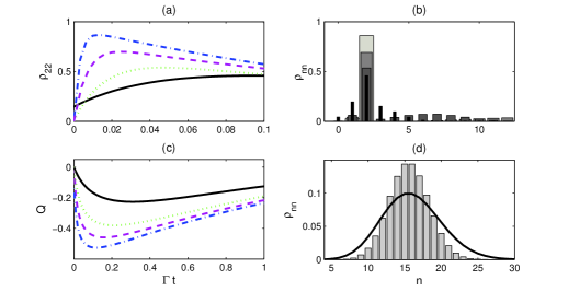
Figure 1: (Color online) Generation of nonclassical states from a coherent state $|\alpha\rangle$ in the presence of linear loss using designed nonlinear dissipation described by the Lindblad operator $A$. Thermal driving is absent, ${\bar{n}}=0$, and the loss ratio is given by $\gamma=\Gamma/5$. I. Generation of the Fock state $|2\rangle$ using nonlinear dissipation given by $A=|2\rangle\langle\alpha|a^{2}$. (a) Fidelity of the target two-photon state as a function of nonlinear loss $\Gamma t$. Solid, dotted, dashed and dash-dotted lines correspond to $\alpha=2,3,4,5$. The panel (b) shows the photon number distribution of the generated state when the fidelity in (a) is maximal; black, dark grey, grey and light bars correspond to $\alpha=2,3,4,5$. II. Generation of sub-Poissonian light and photon-number squeezing using tailored dissipation with $A=a(a^{+}a-1)$. (c) Mandel Q-parameter vs nonlinear loss $\Gamma t$; solid, dotted, dashed and dash-dotted lines correspond to $\alpha=2,4,6,8$. (d) Photon number distribution of the generated state for the minimal Q and $\alpha=8$ (grey bars) in comparison with the Poissonian distribution with the same average number of photons (solid line).

For a linear loss present, a simple physical picture behind the loss-suppression mechanism is provided by system jumps to the lower energy levels. Notably, the rate of transition to the lower levels due to nonlinear dissipation can be much higher than the transition rate due to linear loss. Now, the stationary state of the evolution induced by nonlinear dissipation corresponds to a nonclassical state. Hence when the dynamics due to nonlinear dissipation prevails over that due to linear dissipation, the system is driven into a desired nonclassical state with influence of linear loss being negligible. Designing dissipation (i.e., the Lindblad operator) we determine the form of the nonclassical target state. If we apply this quantum jump formalism to the system desribed by Eqs. (1)-(3), we can deduce that for

$$\Gamma(\bar{n}+1)\langle\Psi|a^{\dagger}a|\Psi\rangle\ll\gamma\langle\Psi|A^{\dagger}A|\Psi\rangle$$ (4)

the influence of the linear loss (and of incoherent driving) during the time of the target state generation is negligible. For a coherent initial state $|y\rangle=|\alpha\rangle$ with sufficiently large amplitude, $\alpha\gg 1$, condition (4) gives $\Gamma(\bar{n}+1)\ll\gamma\mathcal{N}$. In practical terms, for the target state lying within the subspace of Fock vectors with up to $k$ photons, the generation can be nearly perfect and improved further just by increasing the amplitude $\alpha$.

Fig. 1 (a,b) illustrates the solution of Eq.(1) for the generation of the two-photon Fock state from an initial coherent state $|\alpha\rangle$ with the nonlinear dissipation described by the Lindblad operator $A=|2\rangle\langle\alpha|a^{2}$. The rate of nonlinear loss, $\Gamma$, is $5$ times less than the rate of the linear loss, $\gamma$. The incoherent driving is absent. By increasing the amplitude $\alpha$ the target state $|2\rangle$ is approximated with a larger fidelity and over a shorter time period, despite the presence of rather strong linear loss (Fig.1(a,b)).

As we have seen, if for a class of states the jump rate of the nonlinear dissipation far exceeds the jump rate for the linear loss, then an influence of the linear loss is negligible. Moreover, the dynamics due to the engineered nonlinear dissipation can also be non-exponentially fast. For example, for the two-photon dissipation, quite different initial states can decay into the stationary state practically over the same period of time DodMiz . Thus, for an appropriately constructed dissipative gadget it is always possible to combat the linear loss with any pre-defined rate just by choosing the appropriate initial state, in particular, by increasing an average number of photons in the initial state. Of course, there are diffirent practical limitations in construction of dissipative gadgets. However, even for available types of nonlinear dissipative processes it is possible to have significant non-classicality (in particular, large photon-number squeezing) on the time scales when influence of the linear losses is negligible (see, for example, Refs. MS ; valera2011 ). This is illustrated in Fig.1(c, d), where the exact solution of Eq.(1) is shown for the nonlinear dissipation described by the Lindblad operator $A=a(a^{+}a-1)$ in the presence of a linear loss and for an initial coherent state $|\alpha\rangle$. Obviously, this Lindblad operator satisfies condition (4) for a sufficiently large $\alpha$. In the initial stages of evolution, nonclassical states can be generated and the non-classicality (photon-number squeezing in this case) is increased with increasing of the amplitude $\alpha$ in the initial state. Panel (c) shows the Mandel Q parameter confirming that the generated light exhibit the sub-Poissonian statistics (for $Q<0$). Note, that the maximum of non-classicality is reached rather quickly. The generated state then further evolves towards the classical regime under the influence of the linear loss but it happens quite slowly compared to the time required for the nonclassical state generation. This is a rather general feature of the dynamics for any dissipative gadget satisfying condition (4) mikhalychev new .

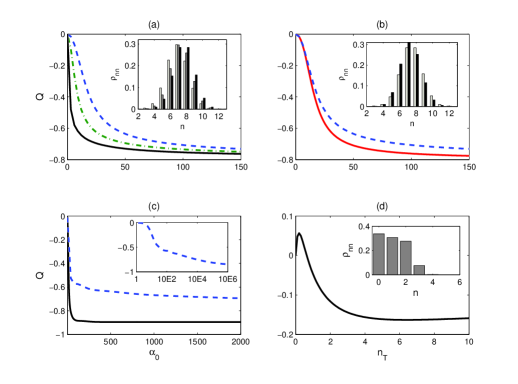
Figure 2: (Color online) Generation of nonclassical states in the long-time limit using nonlinear coherent loss (NCL) to counteract linear loss. (a) Mandel’s Q-parameter vs amplitude of the coherent driving $\alpha_{0}=\Omega/\gamma$ for the NCL with $A=aa^{\dagger}a-1$ provided by the exact solution of Eq.(1); solid, dash-dotted and dashed curves correspond to the relative loss rate $\Gamma=\gamma$, $5\gamma$, $10\gamma$. Inset shows photon-number distribution of the stationary state for $\alpha_{0}=150$; light-grey, grey and black bars correspond to $\Gamma=\gamma$, $5\gamma$, $10\gamma$. (b) Same for the NCL with $A=a(a^{\dagger}a-1)$ for the exact solution of Eq.(1) (dashed line) and for the solution of the approximate equation (Nonlinear dissipation can combat linear loss)(solid line). Inset shows photon-number distributions for the solution of the exact (grey bars) and of the approximate (black bars) equations. (c) Exact (dashed line) and approximate (solid line) solutions for Q-parameter for $A=a(a^{\dagger}a-1)^{2}$; the inset shows long-time behavior of Q-parameter given by the exact solution. (d) Exact solution for Q-factor in dependence of the average number of thermal pumping photons, $n_{T}$; the coherent driving is absent; $A=a(a^{\dagger}a-1)^{3}$.

It might seem surprising, but analogous approach can allow for combating linear losses also in the long-time limit. More precisely, there is a class of nonlinear losses such that for an arbitrarily large (but finite) ratio $\varepsilon=\Gamma/\gamma$ an influence of losses on the stationary state can be completely eliminated by the sufficiently strong coherent driving, and, moreover, even by thermal pumping. Note, that the steady state, while being mixed, can still be strongly non-classical. Consider, for the example, nonlinear coherent loss (NCL) described by the Lindblad operators $A=af(a^{\dagger}a)$, $f(x)$ being a smooth function. This operator is the annihilation operator for the so called ”f-deformed” quantum harmonic oscillator; eigenstates of this operator are reffered to as ”nonlinear coherent states” manko . Any pure state non-orthogonal to an arbitrary Fock states can be exactly represented as a nonlinear coherent state. If it is orthogonal to some Fock states, then one can still devise a nonlinear coherent state closely approximating the state in question kis . NCL can be realized in practice in a number of schemes (for example, with ions or atoms in traps zoll96 ; Bose-Einstein condensates SM or even in multicore nonlinear optical fibres MS . With function $f(x)$ having a finite or countable number of zeros, one can generate Fock states or even ”comb” the initial state by filtering out some pre-defined set of components in the given basis michalychev2011 .

Let us show now that even a weak NCL can be protected from large linear loss and used for generation of non-classical stationary states. We use the classical driving in the form $H=i\Omega(a-a^{\dagger})$ where the parameter $\Omega$ represents the strength of driving and, for simplicity, is taken to be real. For the moment being, the thermal pumping is assumed to be absent, $\bar{n}=0$. Fig. 2 depicts such a non-classicality rescue procedure when generating sub-Poissionian light. Notably, for $A=a(a^{\dagger}a-1)$, the Mandel’s Q parameter $Q=(\langle(a^{\dagger}a))^{2}\rangle-\langle(a^{\dagger}a))\rangle^{2})/\langle(a^{\dagger}a))\rangle-1$ eventually tends to the same limiting value for quite different linear loss rates, $\Gamma=\gamma$, $5\gamma$ and $10\gamma$ (Fig. 2(a)). It is remarkable that the generated states are also quite similar (see inset in Fig.2(a) for the density matrix).

The nature of this phenomenon can be well illustrated and clarified with the help of the following simple approximation. Eq.(1) can be written as

$$\frac{d}{dt}\rho=\gamma a\rho(B^{\dagger}-\alpha_{0})+\gamma(B-\alpha_{0})\rho a^{\dagger}-$$

$$\gamma a^{\dagger}(B-\alpha_{0})\rho-\gamma\rho(B^{\dagger}-\alpha_{0})a-$$ (5)

$$\gamma a[[\rho,f(a^{\dagger}a)],f(a^{\dagger}a)]a^{\dagger}$$

where $B=a([f(a^{\dagger}a)]^{2}+\varepsilon)$. The last term is small in comparison with the others when the inequality $\{f(n)-f(m)\}^{2}\ll 2f(n)f(m)$ holds for all $n$ and $m$, corresponding to essentially non-zero density matrix elements $\rho_{nm}$. For example, for any power-law nonlinearity $f(x)\sim x^{k}$, this condition is satisfied when the driving is sufficiently strong. Neglecting the last term in Eq.(Nonlinear dissipation can combat linear loss), the stationary state, $\rho^{s}$, for Eq.(Nonlinear dissipation can combat linear loss) is the eigenstate of the operator $B$ satisfying $B\rho^{s}=\alpha_{0}\rho^{s}$ and $\rho^{s}B^{\dagger}=\alpha_{0}\rho^{s}$; where $\alpha_{0}=\Omega/\gamma$. This leads to the following recurrence relation for the diagonal (in the Fock-state basis) elements of the steady state:

$$\rho_{n,n}^{s}=\rho_{n-1,n-1}^{s}\frac{\alpha_{0}^{2}}{n(f(n)^{2}+\varepsilon)^{2}}.$$ (6)

Assuming that the steady-state photon number distribution is peaked at $n_{0}$, from Eq.(6) we get a simple condition for determining $n_{0}$:

$$\rho_{n,n}^{s}\approx\rho_{n-1,n-1}^{s}\Rightarrow n_{0}((f(n_{0})^{2}+\varepsilon)^{2})\approx\alpha_{0}^{2}.$$

This condition indicates that for sufficiently strong classical driving and for function $f(n)$ increasing monotonically for sufficiently large $n>0$, one will always have $f(n_{0})^{2}\gg\varepsilon$, and the influence of linear losses on the generated steady state will be negligible. The relation (6) also allows for estimating the width of the photon-number distribution of the stationary state. Assuming that the value of the diagonal element $\rho_{n,n}^{s}$ changes only weakly for small changes $\delta n$ of the photon number $n$ near $n_{0}$, one obtains from Eq.(6) the following expression:

$$\rho_{n_{0}+\delta n,n_{0}+\delta n}^{s}\approx\rho_{n_{0},n_{0}}^{s}\times$$

$$\exp\left\{-\frac{|\delta n|(|\delta n|+1)}{2n_{0}}\left(1+\frac{4n_{0}\dot{f}(n_{0})f(n_{0})}{f(n_{0})^{2}+\varepsilon}\right)\right\}.$$ (7)

From Eq.(7) we can estimate the variance, $\Delta^{2}n$, of the steady-state photon number distribution:

$$\Delta^{2}n\approx n_{0}\left(1+\frac{4n_{0}\dot{f}(n_{0})f(n_{0})}{f(n_{0})^{2}+\varepsilon}\right)^{-1}.$$ (8)

Thus, our approximation shows that in the limit of strong driving the steady state produced by the NCL will always be photon-number squeezed state, provided that $\dot{f}(n_{0})>0$. The squeezing can be quite high. For example, let us use $f(n)=n-1$, which has been proved feasible using three-well potential in Bose-Einstein condensates SM or three-core nonlinear fibers MS . For the simple NCL with $f(n)=n-1$, the value $\Delta^{2}n\rightarrow n_{0}/5$ is asymptotically reached for $n_{0}\approx(\alpha_{0})^{2/5}\rightarrow+\infty$. This value corresponds to the Mandel parameter equal to $-0.8$. Fig. 2(b) shows that the approximation to Eq. (Nonlinear dissipation can combat linear loss) indeed gives rather good estimate for both the Mandel parameter and the generated state. It should be noted though, that for rapidly increasing $f(n)$ the approximation works somewhat worse. It can be easily seen from Eq.(8), since it predicts Q-parameter close to $-1$ for rapidly increasing $f(n)$, e.g., $Q\sim-4k/(4k+1)$ for $f(n)=n^{k}$. $Q=-1$ corresponds to the Fock state. But when the photon number distribution becomes very narrow, the assumption of slowly changing $\rho_{nn}$ near maximum of the photon number distribution can be hardly applied. Nevertheless, the approximation still provides a qualitatively correct description as illustrated in Fig. 2(c) for $f=(x-1)^{2}$, where exact and approximate solutions for Q-parameter are compared. Hence even for $f(x)$ increasing rather rapidly one can indeed have highly pronounced non-classicality unaffected by any linear loss. However, it happens at the expense of quite strong coherent driving required (see Fig. 2(c)).

The essence of our method to preserve non-classicality lies in engineering the evolution to yield a stationary state obeying the following requirement. A stationary state of the master equation for a given system should be such, that the transition rates corresponding to nonlinear loss far exceed transition terms corresponding to linear loss, that is, the condition (4) holds. This simple fact points to the possibility of exploiting not only the coherent driving, but other kinds of driving, too. In particular, the conventional linear thermal driving can protect non-classicality as well, although this seems quite paradoxical. Indeed, in the absence of the coherent driving ($\Omega=0$), from exact Eq.(Nonlinear dissipation can combat linear loss) the following recurrence relation is obtained:

$$\rho_{n}=\rho_{n-1}\frac{\bar{n}}{(\bar{n}+1)+(\gamma/\Gamma)f^{2}(n)}$$ (9)

For small values of $(\gamma/\Gamma)f^{2}(n)$ the state (9) is very close to a thermal state. For $(\gamma/\Gamma)f^{2}(n)\gg(\bar{n}+1)$ the photon number distribution is effectively truncated. The truncation number, $n_{t}$ can be estimated from the following equation: $\bar{n}+1\sim(\gamma/\Gamma)f(n_{t})$. If the density matrix elements $\rho_{n}$ decrease with increasing photon number $n$ faster than for any coherent state: $\rho_{n}/\rho_{n-1}=o(1/n)$, the considered state is nonclassical. Eq.(9) implies that for $f(x)$ growing faster than $x$ this condition is satisfied and the stationary state is nonclassical for any values of system parameters. Fig. 2(d) shows an example of such a ”thermal rescue” for the nonlinear loss with $f(x)=(x-1)^{3}$. Thus, remarkably, the thermal excitation is able to produce photon anti-bunching. However, it is easy to see that the minimal $Q$-value always corresponds to some finite $\bar{n}$.

To conclude, we have shown that dissipative gadgets can be made extremely robust with respect to additional linear losses unavoidably affecting any realistic engineered dissipation scheme. First we have shown that it is always possible to devise a dissipative gadget for the generation of any desired target state starting from the wide class of initial states during the time interval when influence of linear loss is negligible. We provided several examples illustrating such scenario using coherent input states. The larger the difference in average number of photons between the initial state and the target state, the more robust the scheme can be made. Then, by applying conventional linear quasiclassical driving, the non-classicality of the stationary state generated by the dissipative gadget can be preserved. It is remarkable that there exists a class of dissipative gadgets based on the nonlinear coherent loss (NCL), for which the influence of linear loss can be completely annihilated by a sufficiently strong coherent driving. The resulted state is mixed. However, this stationary mixed state can be very close to the Fock state exhibiting strong photon-number squeezing. Furthermore, there exists a class of dissipative gadgets, for which non-classicality of the stationary state can be rescued even by using usual incoherent thermal driving.

This work was supported by the Foundation of Basic Research of the Republic of Belarus, by the National Academy of Sciences of Belarus through the Program ”Convergence”, by the Brazilian Agency FAPESP (project 2011/19696-0) (D.M.) and has received funding from the European Community’s Seventh Framework Programme (FP7/2007-2013) under grant agreement n^∘ 270843 (iQIT).

References

- (1) J. F. Poyatos, J. I. Cirac and P. Zoller, Phys. Rev. Lett. 77, 4728 (1996).
- (2) A. R. R. Carvalho, P. Milman, R. L. de Matos Filho, and L. Davidovich, Phys. Rev. Lett. 86, 4988 (2001).
- (3) B. Kraus, H.P. Buchler, S. Diehl, A. Kantian, A. Micheli, and P. Zoller, Physical Review A 78, 042307 (2008).
- (4) F. Verstraete, M. M. Wolf, and J. Ignacio Cirac, Nature Physics 5, 633 (2009).
- (5) H. Ezaki, E. Hanamura, and Y. Yamamoto, Phys. Rev. Lett. 83, 3558 (1999).
- (6) M. Alexanian, S. K. Bose, Phys. Rev. Lett. 85, 1136 (2000).
- (7) H. Ezaki, E. Hanamura, and Y. Yamamoto, Phys. Rev. Lett. 85, 1137 (2000).
- (8) T. Hong, M. W. Jack, and M. Yamashita, Phys. Rev. A 70, 013814 (2004).
- (9) D. Mogilevtsev and V. S. Shchesnovich, Optt. Lett. 35, 3375 (2010).
- (10) M.B. Plenio, S.F. Huelga, A. Beige, and P.L. Knight, Phys. Rev. A59, 2468 (1999).
- (11) A. S. Parkins and H. J. Kimble, Phys. Rev. A 61 052104 (2000).
- (12) S. Clark, A. Peng, M. Gu and S. Parkins, Phys. Rev. Lett. 91 177901 (2003).
- (13) M. J. Kastoryano, M. M. Wolf, J. Eisert, arXiv:1205.0985v1 [quant-ph](2012).
- (14) F. Pastawski, L. Clemente and J. I. Cirac, Phys. Rev. A 83 012304(2011).
- (15) K. Stannigel, P. Rabl and P. Zoller, New J. Phys. 14 063014 (2012).
- (16) V. V. Dodonov and S. S. Mizrahi, Phys. Lett. A 223, 404 (1996).
- (17) V. S. Shchesnovich, D. Mogilevtsev, Phys. Rev. A 84, 013805 (2011).
- (18) A. Mikhalychev, D. Mogilevtsev, in preparation.
- (19) V.I. Manko, G. Marmo, E.C.G. Sudarshan, and F. Zaccaria, Phys. Scr. 55, 528 (1997); V.I. Manko and R. Vilela Mendes, J. Phys. A 31, 6037 (1998).
- (20) Z. Kis, W. Vogel, and L. Davidovich, Phys. Rev. A 64, 033401 (2001).
- (21) V. S. Shchesnovich, D. S. Mogilevtsev, Phys. Rev. A 82, 043621 (2010).
- (22) A. Mikhalychev, D. Mogilevtsev, S. Kilin, J. of Phys. A: Math. Theor. 44, 325307 (2011).