Influence of lattice disorder on the structure of persistent polymer chains

Abstract

We study the static properties of a semiflexible polymer exposed to a quenched random environment by means of computer simulations. The polymer is modeled as two-dimensional Heisenberg chain. For the random environment we consider hard disks arranged on a square lattice. We apply an off-lattice growth algorithm as well as the multicanonical Monte Carlo method to investigate the influence of both disorder occupation probability and polymer stiffness on the equilibrium properties of the polymer. We show that the additional length scale induced by the stiffness of the polymer extends the well-known phenomenology considerably. The polymer’s response to the disorder is either contraction or extension depending on the ratio of polymer stiffness and void space extension. Additionally, the periodic structure of the lattice is reflected in the observables that characterize the polymer.

1 Introduction

The conformational properties of polymers exposed to disordered media are strongly affected by the surrounding disorder potential. For the case of flexible polymers, the impact of disorder on polymers has already been widely discussed [1–9]. The special case of geometrical constraining environments has been investigated in e.g. [10, 11]. It is expected that geometrical restrictions to chain conformations also play a crucial role for biological systems. In these systems, polymers may no longer be assumed flexible and models of moderately stiff polymers, called semiflexible polymers, are introduced. The stiffness is characterized by the persistence length $l_{p}$. On length scales shorter than the persistence length, the polymers behave like stiff rods, on longer scales they exhibit entropic flexibility and random coiling occurs. The geometrical restrictions of the environment along with the intrinsic stiffness of the polymers lead to an interesting phenomenology, which, in contrast to the case of flexible polymers, is much less understood for semiflexible polymers [10–14].

In this work we examine the equilibrium properties of a pinned semiflexible polymer exposed to a quenched random potential consisting of hard disks. The disks are arranged on the sites of a square lattice. We build up on [11], where flexible polymers exposed to hard-disk disorder assembled on the sites of a square lattice were investigated. We extend the polymer model to comprise bending stiffness. The appropriate polymer model is the Heisenberg chain model. Additionally, we consider the effect of leaving the constraint of a fixed starting point.

The rest of the paper is organized as follows. In section 2 we describe the polymer model and the assumed disorder configurations. Section 3 is devoted to the employed simulation algorithms and in section 4 we define the measured observables, discuss the simulation parameters, and present a few test cases. Our main results are contained in section 5, where we first discuss the low disorder-density case and then the more intricate high-density regime. We conclude this section with a few remarks on the impact of the hard-disk diameter and the initial pinpoint. Finally, in section 6 we summarize our main findings.

2 Model

2.1 Polymer model

Effectively, the Heisenberg chain is a bead-stick model consisting of $N+1$ beads at positions $\mathbf{r}_{i}$ connected by bonds of fixed length $b$. Therefore, the contour has a length of $L=Nb$. Our considerations are made for the case of two dimensions and a phantom chain where self-avoiding constraints are neglected. The connecting line between two monomers defines a unit tangent vector $\mathbf{t}_{i}=(\mathbf{r}_{i+1}-\mathbf{r}_{i})/b$. The elastic properties are governed by the bending energy

$$\mathcal{H}=-J\sum_{i=1}^{N-1}\mathbf{t}_{i}\mathbf{t}_{i+1},$$ (1)

where $\mathbf{t}_{i}\mathbf{t}_{i+1}=\cos(\theta_{i,i+1})$ determines the angle between neighboring bonds and $J>0$ is a coupling constant. The correlations between the two-dimensional tangent vectors of the free Heisenberg chain decay at inverse temperature $\beta=1/k_{\mathrm{B}}T$ as [15]

$$\langle\mathbf{t}_{i}\mathbf{t}_{i+k}\rangle=\left[\frac{I_{1}(\beta J)}{I_{0}(\beta J)}\right]^{k},$$ (2)

where $I_{\mu}(x)$ is the modified Bessel function of the first kind of order $\mu$.

Carrying out the continuum limit of the Heisenberg chain by taking (1) and letting $N,J\rightarrow\infty$ while $b\rightarrow 0$ with $Jb=\mathrm{const}.$ and $Nb=L$ (constant length constraint), transfers (1) up to a constant into

$$\mathcal{H}=\frac{\kappa}{2}\int_{0}^{L}ds\left(\frac{\partial^{2}\mathbf{R}(s)}{\partial s^{2}}\right)^{2}$$ (3)

with $\kappa=Jb$ being the bending stiffness and $\mathbf{R}(s)$ describing the contour parametrized by arc length $s$. Equation (3) is the Hamiltonian of the worm-like chain, also called Kratky-Porod model [16], one of the most famous and widely spread models for treating semiflexible polymers analytically.

A central property of the worm-like chain is its persistence length $l_{p}$, which is the tangent vector correlation length [17],

$$\langle\mathbf{t}(0)\mathbf{t}(s)\rangle=e^{-s/l_{p}},$$ (4)

where $\mathbf{t}(s)=\partial\mathbf{R}(s)/\partial s$. In the continuum limit of the Heisenberg chain Hamiltonian, we consider the following approximation. For large $\beta J$ or small $b$, and therefore large $N$, the modified Bessel function in (2) yields [18]:

$$I_{\mu}(x)\approx\frac{e^{x}}{\sqrt{2\pi x}}\left\{1-\frac{4\mu^{2}-1}{8x}+\frac{(4\mu^{2}-1)(4\mu^{2}-9)}{2!8x^{2}}-\mathcal{O}(x^{-3})\right\}.$$ (5)

Thus, for large $\beta J\propto N$ and $l=kb$ one finds for the tangent correlations by inserting (5) into (2) to leading order:

$$\langle\mathbf{t}_{i}\mathbf{t}_{i+k}\rangle=\mathrm{exp}\left(-\frac{k_{B}T}{2Jb}l\right).$$ (6)

A comparison of (6) with (4) and identifying $l$ with $s$ results in

$$l_{p}=2\frac{Jb}{k_{B}T}=2\frac{\kappa}{k_{B}T}.$$ (7)

The persistence length is thus the ratio between bending stiffness $\kappa$ and thermal energy $k_{B}T$ and is therefore a measure of the stiffness of a polymer. In general dimension $d$ it holds [19]:

$$l_{p}=\frac{2}{d-1}\frac{\kappa}{k_{B}T}.$$ (8)

There are three regimes defining three classes of polymers:

$$\left\{\begin{array}[]{ll}b\approx l_{p}\ll L&\mathrm{flexible}\\ b\ll l_{p}<L&\mathrm{semiflexible}\\ b\ll L\ll l_{p}&\mathrm{stiff}.\\ \end{array}\right.$$ (9)

At last we want to remark on the mean square end-to-end distance $\langle R_{\rm ee}^{2}\rangle$. Using the definition $\langle R_{\rm ee}^{2}\rangle=\langle(b\sum_{i=1}^{N}\mathbf{t}_{i})^{2}\rangle$ together with (2), its calculation is straightforward and amounts in the continuum limit to (cp. e.g. [17]):

$$\langle R_{\rm ee}^{2}\rangle=2l_{p}L\left\{1-\frac{l_{p}}{L}[1-\exp(-L/l_{p})]\right\}.$$ (10)

2.2 Disorder

The background potential consists of hard disks with diameter $\sigma$ that interact with the monomers of the polymer via hard-core repulsion described by the potential

$$V=\left\{\begin{array}[]{l l}\infty&\quad\mathrm{for}\quad d<\sigma/2\\ 0&\quad\mathrm{else}\end{array}\right.,$$ (11)

where $d$ is the distance between a monomer and a hard-disk center. Thus, the monomers—here described by points—may not be placed onto the area of a disk.

The assembly of the disks is the same as in [11]. The disks are put onto the sites of a square lattice with lattice constant $a$. Each site is occupied with a certain occupation probability $p$ independent of the other sites. Consequently, there is no interaction between neighboring disks besides the constraint that the minimum distance between two disk centers is $a$, the lattice constant. This leads to clustering and hence a spatially inhomogeneous structure of obstacles [20].

3 Algorithms

As in [11], we apply two algorithms for double-checking our results. One is an off-lattice growth algorithm proposed by Garel and Orland [21] and one is the multicanonical Monte Carlo method [22–24]. Here, we only concentrate on those aspects which are relevant for the semiflexible case. Otherwise we refer to [11].

For the multicanonical approach we have developed in [11] a special modification, allowing us to reweight to different background potential amplitudes. To this end, we replace the infinite hard-disk potential with finite potential steps and after performing the multicanonical simulation at fixed persistence length, we are able to reweight to any potential amplitude ranging from the free polymer (zero amplitude) to the polymer in a hard-disk background (very large amplitude).

The basic routine of the growth method—also called replication-deletion procedure (RDP)—is comprised in figure 1. Polymers are grown in parallel from an initial starting point. In each step, a polymer configuration is cloned according to the Boltzmann weight $w_{i}$ for adding a new monomer. $i_{i}=\mathrm{Int}(w_{i})$ is defined as the integer part of $w_{i}$ and $r_{i}=w_{i}-i_{i}$ as the rest. Replicating the new chain $w_{i}$ times statistically means replicating it $i_{i}$ times plus one additional time with probability $r_{i}$. Therefore a random number $r$ with $0\leq r\leq 1$ is drawn. If $r\geq r_{i}$, the chain is replicated $i_{i}$ times. Otherwise it is replicated $(i_{i}+1)$ times. Since $w_{i}$ can be smaller than 1, the replication can in fact amount to a deletion. This is why the method is called replication-deletion-procedure. The different clones are treated as independent polymer configurations and are grown until the desired degree of polymerization is reached. In dependence on the Hamiltonian of the system, cloning the configurations according to the Boltzmann weight leads—except for very simple situations—to either exponential increase of the numbers of configurations or to dying out of almost all configurations. Both cases defy the estimation of meaningful numerical averages. This problem can be overcome by introducing a population control parameter (PCP), ensuring that the number of sampled configurations $\mathcal{M}_{N}$ roughly coincides with the initial number of chains $\mathcal{M}_{1}$. For the principle of the PCP, we refer to the original paper by Garel and Orland [21] and to [11].

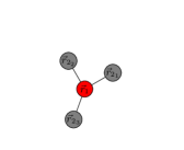
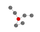
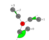
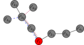
(a)	(b)	(c)	(d)	(e)

Figure 1: (Color online) (a) $\mathcal{M}_{1}$ monomers at position $\mathbf{r}_{1}$. The first monomer—here marked by —thus stands for $\mathcal{M}_{1}$ (three in this example) different chains of zero length.
(b) Each of the $\mathcal{M}_{1}$ chains is extended by one monomer. There are now $M_{2}=3$ independent chains of length one. Up to now, there is no energy term as there is no bending angle between neighboring bonds.
(c) Each of the $M_{2}$ chains is extended by one monomer. There are now $M_{3}=3$ independent chains of length two.
(d) Now, energy comes into play as there is a bending angle between the first and second bond of the polymers. Temperature $T$ and coupling constant $J$ are chosen such that they yield the weights that are given in the sketch ($\times 3,\times 1,\times 0$). Each of the chains is replicated according to its weight. Accordingly $M_{3_{\rm new}}=4$. There are now four independent chains of length two.
(e) Each of these chains is extended independently by one monomer and bond. This procedure is iterated until the desired degree of polymerization is reached.

The RDP generates a population of chains that is Boltzmann distributed. To be more precise, this procedure provides such a distribution in every single growth step. A strong advantage thereof is to be able to do a scaling analysis within one simulation. Having a distribution of chains of length $N$ automatically provides all the distributions of length $\tilde{N}=1,\ldots,N$. We found by comparison with the multicanonical method that correlations due to the growth process which would pass a possible bias from ensembles of short chains to those of longer chains can largely be excluded. More on the correlations of chains will be discussed in section 3.1.

Although getting distributions of all lengths up to the desired degree of polymerization within one simulation is an advantage for scaling analyses, it might be a drawback concerning the question of ergodicity. Depending on the choice of the potential, the polymer chain might, for example, get stuck in a local energy minimum which hinders the chain from sampling phase space evenly enough to provide a Boltzmann distributed population of chains that satisfies the ergodicity condition.

This drawback can be cured by introducing a guiding field that locally makes the distribution of chains non-Boltzmann distributed thus facilitating to sample phase space more uniformly by forcing the chain to circumvent or get out of local energy minima [21]. A second aspect of the guiding field is to make the algorithm much more efficient. Here, we bias the distribution of chains by drawing angles not uniformly but from another distribution which is inspired by the nature of the problem. Afterwards, the weights have to be adapted such that the resulting distribution is unbiased. The guiding field is made up of two parts, one accounting for the bending energy of the polymer and one for the disks of the background potential.

(a)	(b)

Figure 2: (Color online) Background-aware guiding field.

Assume a situation as sketched in figure 2(a), where a polymer with a certain bending stiffness grows in the direction that is indicated by the arrow (red). The hatched disk is an obstacle located in the growth direction. The dashed (green) line indicates the guiding field based solely upon the bending stiffness. Both the guiding field and the Boltzmann weight favor a growth in the direction of the bond indicated by the arrow and thereby in the direction of the obstacle. The polymer does not sense the obstacle until it is one bond length away of it. It is obvious that only a large bending angle can prevent the polymer from overlapping with the obstacle. Depending on the bending stiffness, the resulting weight will be rather small and the configuration does not contribute a lot or might even die out. This problem is based upon the update routine that only takes into account its directly surrounding area.

A way to overcome this problem is to introduce a guiding field that takes into account the obstacles in the vicinity of the growing end of the polymer. Such a guiding field is depicted in figure 2(b). The probability of choosing an angle that leads in the direction of an obstacle is reduced [framed (black) curve]. The corresponding probability density considers only disks within a certain distance and adds for each disk a Gaussian dip with a certain amplitude and variance. The form of the probability density and the parameters are determined empirically and by intuition. Both amplitude and variance are a function of the distance between obstacle and monomer as well as of the persistence length. The emerging growth direction is a superposition of the contributions from the persistence of the polymer and from the surrounding potential. It is evident that a polymer with a larger persistence length has to sense the obstacles more in advance than one with a smaller persistence length, because the probabilistic suppression of certain angles depends exponentially on the bending stiffness.

3.1 Averaging and error estimation

We consider the background to be static on the timescale of polymer fluctuations. This is taken into account by performing the quenched disorder average for calculating observables. Therefore two averages have to be carried out. The first is an average over polymer configurations belonging to a single disorder realization. It is written in angular brackets $\langle\ldots\rangle$. This is done for all disorder realizations and the quenched average is calculated thereof by averaging over the measured values of the single disorder realizations. The polymer configurations that belong to a single disorder realization are all pinned at the same pinpoint. Leaving the constraint of the pinpoint is discussed in section 5.4. The quenched average is written as $[\langle...\rangle]$.

Consequently, two kinds of variances have to be considered, one from the average of polymer configurations within a single disorder realization, and the other from the average over different disorder realizations. These two contributions amount in an effective variance $\sigma_{\rm eff}^{2}$ which is estimated by (see e.g. [25]):

$$\sigma_{\rm eff}^{2}=\frac{\sigma_{\mathcal{O}}^{2}}{N_{r}},$$ (12)

where $\sigma_{{\mathcal{O}}}^{2}$ is the variance of the Monte Carlo mean values over a finite sample of $N_{r}$ different (independent) disorder realizations. For the error bar we take the standard deviation $\sqrt{\sigma_{\rm eff}^{2}}$. For the case of fixed pinpoints, the quenched average is carried out over $N_{r}=1500$ independent disorder realizations. With this statistical precision, the relative error turned out to be of the order of $1\%$, which is far smaller than the effect of the disorder on the observables. For the scales considered here, the error bars are covered by the plot markers. Therefore we omit them.

In order to achieve a reasonable balance between the amount of computing time invested in the polymer statistics for a given disorder realization and the number of independent disorder realizations, at least a rough estimate of the statistical error of the polymer simulations is needed. The estimation of this error for a simulation within a single disorder realization for the case of the multicanonical Monte Carlo method is well described in literature, e.g. [25]. Things are more complicated for the case of the growth algorithm. There, the different polymer configurations cannot be assumed independent. If we recall the principle of the algorithm, we realize that many polymers share a certain part of their configuration which leads to correlations in the final ensemble. Once having found the number of independent configurations, the error can be estimated after (12). For the free polymer, we follow the approach of Higgs and Orland in [26]. They estimated the variance by assuming that interactions are only between nearest neighbors. As the free polymer model (no disorder) within this work only includes bending energy between neighboring bonds, it fulfills the preconditions of the error estimation by Higgs and Orland. Under this assumption they found the number of independent chains $c_{\rm ind}$ to be proportional to $\mathcal{M}_{1}/N$, where $\mathcal{M}_{1}$ is the initial number of chains and $N$ the number of bonds. The variance of the simulation of a free single chain is calculated by applying (12) with $\sigma_{\rm eff}^{2}$ substituted by the variance of the mean value of a single simulation $\tilde{\sigma}_{\overline{\mathcal{O}}}^{2}$ and $\sigma_{\mathcal{O}}^{2}$ substituted by the fluctuations of the chains belonging to a single simulation $\tilde{\sigma}_{\mathcal{O}_{j}}^{2}$. The number of realizations $N_{r}$ is substituted by the independent number of chains which—according to [26]—yields:

$$\tilde{\sigma}_{\overline{\mathcal{O}}}^{2}\sim\frac{\tilde{\sigma}_{\mathcal{O}_{j}}^{2}}{\mathcal{M}_{1}/N},$$ (13)

where $\tilde{\sigma}$ indicates the case of a single simulation without disorder and without quenched average. The error bars are again taken to be the standard deviation calculated from (13). If we add disorder, the estimation of the number of uncorrelated configurations becomes more difficult as the narrow channels between neighboring disks, especially for high area occupation probabilities, bring about additional correlations. We assessed the necessary number of polymer chains for producing averages in appropriate accuracy by considering the mean values for increasing number of chain configurations.

For all ranges of disorder occupation and persistence length, we found the maximum relative deviations of the mean values for $\mathcal{M}_{1}=50000$ and $\mathcal{M}_{1}=100000$ to be about $5\%$ while the relative deviations for $\mathcal{M}_{1}=100000$ and $\mathcal{M}_{1}=400000$ are only about $1\%$. As the deviations between the latter two are much below the effect of the influence of the disorder, the accuracy obtained by simulating with $\mathcal{M}_{1}=100000$ is completely satisfactory for the scope of this work. The above estimation is reassured by a crosscheck with a completely different method—the multicanonical Monte Carlo method.

4 Observables, parameters, and test cases

4.1 Observables

Throughout this work we focus on two observables: the end-to-end distribution $P(r)$ and the tangent-tangent correlations $\langle\mathbf{t}(0)\mathbf{t}(kb)\rangle$ The end-to-end distribution gives the probability to find a certain end-to-end distance $r=b|\sum_{i=1}^{N}\mathbf{t}_{i}|$. The tangent-tangent correlation function $\langle\mathbf{t}(0)\mathbf{t}(kb)\rangle$ is estimated by averaging the mean tangent-tangent correlation functions of a single polymer configuration over all sampled configurations $N_{p}$ ($\mathcal{M}_{N}$ for the growth algorithm)

$$\langle\mathbf{t}(0)\mathbf{t}(kb)\rangle=\frac{1}{N_{p}}\sum_{j=1}^{N_{p}}\left(\overline{\mathbf{t}_{0}\mathbf{t}_{k}}\right)_{j}=\frac{1}{N_{p}}\sum_{j=1}^{N_{p}}\left(\frac{1}{N-k}\sum_{i=1}^{N-k}\mathbf{t}_{i}\mathbf{t}_{i+k}\right)_{j}.$$ (14)

The tangent-tangent correlation function is a measure of the stiffness of a polymer. For a completely flexible free polymer there is no energetic preference to any angle and hence there are no correlations between tangent vectors for $k\neq 0$. For the case with bending stiffness, the tangent correlations are described by (2). The surrounding disorder can lead to both correlations and anti-correlations [as can be seen later in figure 5(b)].

4.2 Simulation parameters and length scales

The polymer determines three length scales of the system. The total length $L$, the persistence length $l_{p}$, and the bond length $b$. The former two are reduced to the ratio $\xi=l_{p}/L$, which is the persistence length measured in units of polymer length $L$. The persistence lengths considered here include $\xi=0$, representing the flexible case, and $0.1,0.2,0.3,0.5,0.7,1$. The contour length $L$ and the bond length $b$ are related by $Nb=L$, so that $b$ resp. $N$ sets the scale of discretization. In our case, the discrete polymer model has $N=29$ bonds which corresponds to $N+1=30$ monomers. As stated in section 2.1, the polymer is a phantom chain, i.e., there is no steric self-interaction of the chain (the monomers are considered pointlike). The issue of discretization is touched in section 4.3.1.

The simulations are done in a square box with periodic boundary conditions filled with a $20\times 20$ lattice with lattice constant $a$. We consider the site occupation probabilities $p=0,0.13,0.25,0.38,0.51,0.64,0.76,0.89,1.00$. The occupation probabilities are specified to be consistent with those from [11], where they were chosen to equal the area fractions $\rho=0,0.1,\cdots,0.7,0.785$ for $\sigma=a$. The diameter of the disks here is set to $\sigma=0.9a$, which introduces a small channel between neighboring disks. The issue of $\sigma=a$ and $\sigma>a$ is briefly discussed in section 5.3. Unless otherwise stated, the numerical results refer to the case of $\sigma=0.9a$.

The disorder brings another two length scales into play. One is the disk diameter $\sigma$, another is the average free distance between the centers of the disks $l_{0}$. $l_{0}$ is connected to the occupation probability $p$ via $l_{0}=a/\sqrt{p}$, where $a$ is the lattice constant. For our parameter choice ($\sigma=0.9a$) this amounts to

$$l_{0}=\frac{1.11\sigma}{\sqrt{p}}.$$ (15)

Note that $l_{0}$ does not account for the extension of the disks. The top of table 1 gives an overview over $l_{0}$ in dependence on the occupation probability $p$.

The length scales of the polymer and those of the disorder are connected via $L=6.4\sigma$ or, equivalently, $\sigma=4.5b$ (for our choice $N=29$). Note that $a=5b$, which amounts to an effective distance of half the bond length between neighboring disks. For a better comparison of the length scales, the bottom of table 1 shows the persistence length $l_{p}$ of a free polymer in units of $\sigma$.

The simulation parameters are chosen such that we can investigate both the effect of the smallest structures and the impact of the disorder on the polymer on the length scale of several disk diameters $\sigma$. Going to much larger chains at the same accuracy involves a much higher computational effort. The effects we are looking at would, however, be qualitatively the same.

Table 1: Top: Average distance between the centers of the disks in dependence on the occupation probability $p$. Bottom: Persistence length and root mean square end-to-end distance of a free polymer in units of $\sigma$ in dependence on $\xi$.

• $p$	0.13	0.25	0.38	0.51	0.64	0.76	0.89	1.00
  $l_{0}$	$3.1\sigma$	$2.2\sigma$	$1.8\sigma$	$1.5\sigma$	$1.4\sigma$	$1.3\sigma$	$1.2\sigma$	$1.1\sigma$

• $\xi$	0.1	0.2	0.3	0.5	0.7	1.0
  $l_{p}$	$0.64\sigma$	$1.3\sigma$	$1.9\sigma$	$3.2\sigma$	$4.5\sigma$	$6.4\sigma$
  $\sqrt{\langle R_{ee}^{2}\rangle}$	$2.7\sigma$	$3.6\sigma$	$4.2\sigma$	$4.9\sigma$	$5.2\sigma$	$5.5\sigma$

4.3 Test cases

4.3.1 The free polymer

The free semiflexible polymer is already widely discussed throughout literature [17, 27–31]. Here we will just mention some characteristics as the free case will always serve as reference for the case with disorder.

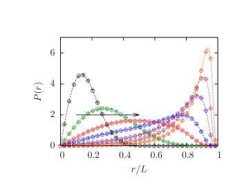
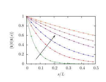
(a)	(b)

Figure 3: (Color online) End-to-end distribution function (a) and tangent correlation function (b) of free semiflexible polymers with $N+1=30$ monomers. The persistence lengths include $\xi=0,0.1,0.2,0.3,0.5,0.7,1$ (increasing persistence indicated by the arrow).
(a): $\circ$ are data from the growth method; $+$ are Metropolis data. The connecting lines are drawn for better visibility.
(b): The solid lines are the analytical solution of the tangent-tangent correlations (2). The trivial case of $\xi=0$—immediate decorrelation—is not shown.

Figure 3 shows the measured observables from section 4.1—the radial distribution function $P(r)$, figure 3(a), and the tangent-tangent correlations $\langle\mathbf{t}(0)\mathbf{t}(s)\rangle$, figure 3(b). The functional form of the end-to-end distribution function $P(r)$ of the free polymer is characterized by a single peak whose position depends on the stiffness of the polymer. The probability of extended chain configurations increases with increasing stiffness. Hence the peak is shifted to the right for increasing bending energy. The tangent-tangent correlations are shown in figure 3(b) and cover the solid lines from (2) perfectly. For the case of no persistence, the tangent-tangent correlation function drops immediately to zero as there is no correlation between the bonds besides the trivial self-correlation at $s=0$.

An important aspect for comparison with analytical work on the worm-like chain model is the degree of discretization of the polymer. Figure 4 shows the tangent-tangent correlation function of a free semiflexible polymer at $\xi=0.2$. The deviations from the continuous case are shown. In the limit of small $b$ or large $\beta J$, and therefore large $N$, the continuous case—exponential decay of the tangent-tangent correlations (6)—is recovered.

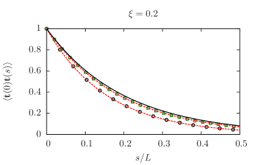
Figure 4: (Color online) Tangent-tangent correlation function of a free semiflexible polymer. $\bigodot$ for the case of 30 monomers and $\boxdot$ for the case of 100 monomers. The dashed lines show the analytical solution (2) of the tangent-tangent correlations for the discrete case. The solid line shows the analytical solution (4) resp. (6) for the continuous case.

4.3.2 Single disorder configuration

We are now adding obstacles to the system. Before we look at the quenched average, we consider three exemplary pinpoints within an artificial disorder configuration, where all sites are occupied except a $4\times 4$ square. Figure 5 illustrates the case with persistence paradigmatically for $\xi=0.5$.

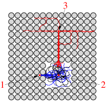
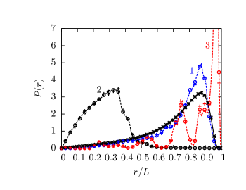
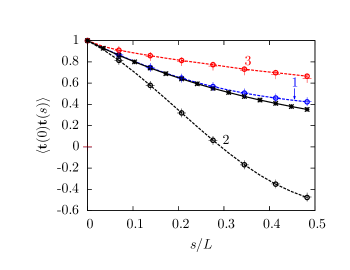
(a)	(b)

Figure 5: (Color online) Top: Distribution of disks with three exemplary pinpoints. The sketch additionally shows a selection of strongly contributing polymer configurations.
Bottom: End-to-end distribution (a) and tangent-tangent correlations (b) that belong to the pinpoints shown above (single simulation; no disorder average) for $\xi=0.5$. $\circ$ shows the data from the growth algorithm; $+$ are data from the multicanonical simulation. The labeling of the curves is given in the plot. The curve marked by $\ast$ shows the free case. The connecting lines are drawn for better visibility.

We start by discussing the issue of pinpoint 1. While the only determining factor for the case without bending energy was entropy, energy gains more and more importance as soon as we start to increase the persistence length. The gain in entropy for configurations pinned to pinpoint 1 by exploring the large free area around pinpoint 2 favors configurations that reach to that space. Going straight through the channel from pinpoint 1 to the free area is even forwarded by the energetic preference for small bending angles. Figure 5(a) and (b) demonstrate that both the end-to-end distribution function and the tangent-tangent correlation function for the case of pinpoint 1 are similar to the free polymer. This is reasonable as the space available for the polymer to spread, once having passed the narrow channel from pinpoint 1 to the adjacent region, provides entropically similar space as for a free polymer. Space for bending back is strongly limited by the potential but as this is energetically not opportune anyway, it does barely affect the equilibrium ensemble. This behavior changes if we move on to configurations starting from pinpoint 2. While this pinpoint provided good preconditions for a flexible polymer to behave as its free counterpart (see [11]), a free polymer with $\xi=0.5$ has a mean extension of about $4.9\sigma$ (cp. table 1). The free space in each direction from pinpoint 2 is about $2\sigma$ which truncates a large part of configuration space. While the confinement forces the polymer to crumple up, the energetic cost for bending stretches the polymer out. The interplay of these effects leads to the formation of loops with strong anticorrelations on the length scale of the persistence length, which is half the polymer length [see figure 5(b)]. Although configurations starting from pinpoint 1 are similar to the free case, configurations starting from pinpoint 2 are “flexibilized”. In contrast, configurations starting from pinpoint 3 show the very reverse—stiffening by disorder. The energetic drive to stretch the polymer allows for finding favorable spots even if they are far away which is just opposite to the flexible case. The large area around pinpoint 2 facilitates a spread of the chain which leads to a strong entropy gain. Therefore, the equilibrium ensemble is strongly dominated by configurations that end in the large free space. Accordingly, the end-to-end distribution is peaked around almost completely stretched configurations and the bonds are strongly correlated on all lengths, which can be seen in figures 5(a) and (b). Some less distinct peaks stem from configurations that are kinked once, twice, etc. The contribution of those configurations quickly decreases with increasing number of kinks, because each kink strongly increases the bending energy.

Now that we have investigated different scenarios that can occur during the quenched average and thus gained insight into some dominating elements of the quenched average, we move on to averaging over many disorder realizations.

5 Results

In [11] the crossover between a low- and a high-density regime is determined by the occupation $p_{0}$ where the mean end-to-end distance of the polymer equals the average distance between neighboring disks. This estimation works better for the case without persistence because the polymers for the case with bending stiffness are more extended in linear shapes, especially for large persistence lengths. We will see that the high-density regime is characterized by a multiple peak structure in the end-to-end distribution function. The beginning of this effect shows up as a small bulge in the end-to-end distribution function. This effect even increases for the case with persistence.

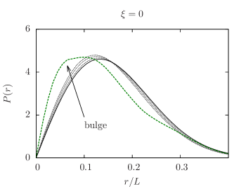
Figure 6: (Color online) End-to-end distribution function for the case of no persistence. The occupation probabilities are $p=0,0.13,0.25,0.38$, and $0.76$ (indicated by the arrow). The solid and dotted (black) curves are in the low-density regime. The high-density case $p=0.76$, labeled by the long-dashed (green) curve, is indicated by a deviation of the functional form from the $p=0$ (black solid) case.

Figure 6 shows the end-to-end distribution function of a flexible polymer in hard-disk disorder. The solid and dotted (black) curves are in the low density regime. The low-density distributions all have the same functional form which is characterized by a single peak. The dashed (green) curve for high-density disorder differs from this structure—it has a bulge. The shape of the bulge that emerges as soon as a certain occupation $p_{0}$ is crossed can be used as indicator to mark the crossover from a low-density to a high-density regime. Similar effects can be observed for the tangent-tangent correlations. We take the qualitative change of the functional form of the end-to-end distribution—formation of double/multiple peak structure—as a qualitative signal for the crossover from a low- to a high-density regime.

5.1 Low-density regime

In the low-density regime, the relevant parameter is the persistence length and not the disorder density. Figure 7 shows the measured data for increasing persistence (growing $\xi$ is indicated by the arrow). The occupation probabilities in the plot are $p=0,0.13,0.25,0.38,0.51$, corresponding to an average distance between the disks of $l_{0}\geq 1.5\sigma$ (cp. table 1).

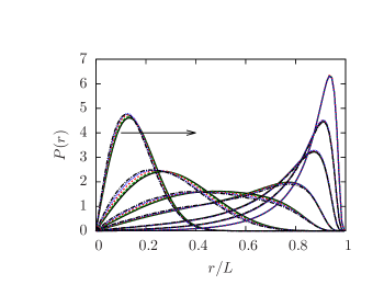
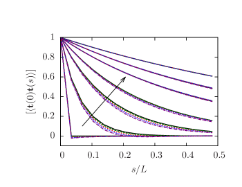
(a)	(b)

Figure 7: (Color online) End-to-end distribution (a) and tangent-tangent correlations (b) in the low-density regime. The persistence lengths include $\xi=0,0.1,0.2,0.3,0.5,0.7,1$ (indicated by the arrow). The occupation probabilities are $p=0$ (, black), $0.13$ (, green), $0.25$ (, red), $0.38$ (, blue), and $0.51$ (, black).

We find two kinds of response to the disorder depending on the stiffness of the polymer—compression and extension. The probability for shorter end-to-end distances is growing for increasing occupation $p$ at low persistence lengths $\xi\leq 0.2$ corresponding to $l_{p}\leq 1.3\sigma$ which is less than the smallest average mean distance $l_{0}=1.5\sigma$ within this density regime. The reverse is observed for $\xi\geq 0.5$ which corresponds to $l_{p}\geq 3.2\sigma$ which is more than the largest average distance $l_{0}=3.1\sigma$ (except for $p=0$) in the low-density regime (the effect of stiffening is hardly seen in figure 7). Remember that higher probability for shorter chains in the end-to-end distribution function [figure 7(a)] and faster decay of the tangent correlations [figure 7(b)] indicate softening. The reverse effect is analogous.

For an explanation of the softening and stiffening at different persistence lengths consider figure 8(a). The case of small persistence lengths is shown on the left in figure 8(a). The energetic cost for bending is in a range where it is more favorable for the polymer to crumple up in order to gain entropy than to stretch. This is different for stiffer polymers. The probability for bending decreases exponentially with increasing persistence. That is why configurations are favored that find tube-like free regions. The width of thermal fluctuations of those configurations is limited by the distance between neighboring disks [right in figure 8(a)]. The squared width of the fluctuations is related to the persistence length via (refer to, e.g., [32])

$$\frac{\delta r_{\perp}^{2}}{L^{2}}\propto\frac{1}{\xi},$$ (16)

i.e., it decreases for increasing persistence length. A large persistence length hence corresponds to a small fluctuation width. Thus, in the limit of large bending stiffness, the stiffening effect induced by disorder vanishes.

$\xi$ small	$\xi$ large	$\xi$ small	$\xi$ large
(a)		(b)

Figure 8: (Color online) Sketch to elucidate the idea of softening and stiffening for persistent polymers at low (a) and high (b) occupation probabilities, respectively. The double-headed arrow indicates the width of the thermal fluctuations of the polymer.

5.2 High-density regime

We now turn over to the high-density regime with $p\geq 0.64$ (which is above the percolation threshold $p_{c}=0.5927$) where the shape of the distributions starts to exhibit characteristics of the potential up to the point where the potential completely dominates the distributions. This means that the confinement increases in such a way that the polymer either has to crumple up even though this is connected to high cost in energy or has to stretch at the expense of entropy.

We consider the effect of high-density disorder for three exemplary persistence lengths, $\xi=0.1$, $0.3$, and $1$. $\xi=0.1$ represents a quite flexible polymer that can well adapt to the surrounding disorder by crumpling up. $\xi=1$ is rather stiff with respect to the disorder and adapting to confinement by crumpling is only feasible at high energetic cost. In this case, adapting is mostly done by stretching. $\xi=0.3$ is in between and exhibits both, crumpling and stretching. The influence of the disk diameter is discussed at the end of this section.

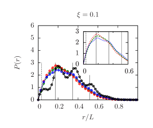
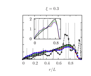
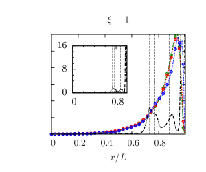
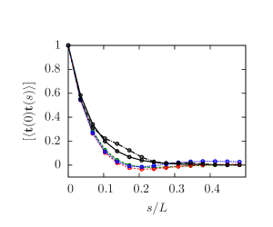
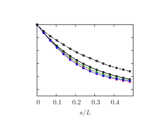
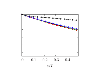
(a)	(b)	(c)

Figure 9: (Color online) End-to-end distribution function (top) and tangent correlation function (bottom) for $\xi=0.1$ (a), 0.3 (b), and 1 (c). The occupation probabilities are: $p=0$ (, black), $p=0.64$ (, green), $0.76$ (, red), $0.89$ (, blue), and $1$ (, black). The vertical lines in the end-to-end distribution functions correspond to the distances shown in figure 10.

In contrast to the low-density regime, the distributions in the high-density regime feature a variety of peaks due to the confining effect of the potential. The periodic structure of the lattice is mirrored in the observables that characterize the polymers.

5.2.1 Small persistence length

The end-to-end distribution and the tangent-tangent correlations for $\xi=0.1$ are shown in figure 9(a). As long as the persistence length is of the order of the extension of the available space, the polymer crumples up close to its pinpoint.

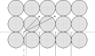
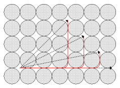
(a)	(b)

Figure 10: Section of a lattice. The part shown here is fully occupied, which is just exemplary. (a): The long-dashed vertical line (left most) is a reference line. The other lines and arrows show different distances on the lattice. The short-dashed vertical line stands for the mean extension in a small cavity. The next vertical line depicts the distance one lattice constant $a$ apart, the next $2a$, and so on. (b): The horizontal arrow indicates the end-to-end distance of fully stretched polymers which are prevailing for large $p$ and $\xi$. The other arrows are end-to-end distances to cavities that are reached by polymers with one $90^{\circ}$ turn. Three of them are indicated by the dashed (red) lines.

The persistence length $\xi=0.1$ corresponds to three bonds. This is of the order of the extension of the smallest cavities (like those around pinpoint $1$ in figure 5; we call them $\diamond$-cavities as they are shaped like a diamond $\diamond$). The left part of figure 8(b) illustrates this situation. Crumpled configurations are reflected in the contributions to small extensions in the end-to-end distribution function [top of figure 9(a)]. Another indicator is a sharper decline of the tangent-tangent correlations [bottom of figure 9(a)]. The peaks in the end-to-end distribution become more pronounced with increasing occupation probability $p$. Some configurations (the fraction of those increases with increasing $p$) will extend to neighboring regions once the energetic penalty for bending becomes too large or it is entropically more favorable for the polymer to extend to neighboring cavities, respectively. The latter situation plays a crucial role especially for flexible polymers [11, 33, 34].

As soon as the $\diamond$-cavities contribute the dominant part to the starting points, especially for the case of $p=1$, the peaks in the end-to-end distribution function can directly be ascribed to the periodic structure of the lattice. Figure 10(a) shows the different length scales that mainly determine the extension of the polymer in this case. Large clusters of void space do not play a role in this regime. The polymer, starting at one point, will either stay near the region where it started or extend through a channel to a neighboring or next-nearest neighboring, etc., free region. The first distance, indicated by the short-dashed vertical line in figure 10(a), plays a role for very high occupation probabilities ($p=0.89,1$), as most of the chains will start in a small cavity. The lines of figure 10(a) are sketched in figure 9 (lines left of 0.6). The dotted lines (arrows) play a subordinate role and are therefore omitted in figures 9 and 11. The reason is that a polymer that moves on to a neighboring cavity instead of staying in the current one has lower energy if it goes straight, which is not the case for the cavities indicated by the arrows. Their role becomes even less important with increasing bending stiffness.

5.2.2 Large persistence length

Next we are looking at the stiff counterpart. Figure 9(c) shows the case of $\xi=1$, which is a typical representative of semiflexible polymers [cp. (9)], where bending on the length scale of a few bonds is punished by high energetic cost. The end-to-end distribution function for $\xi=1$ also exhibits the periodic structure which is preset by the structure of the potential. It is, however, much less pronounced and most of the contributions stem from extended chains. The right of figure 8(b) is an illustration of a polymer with a persistence length that is larger than the average void-space cluster size. Some configurations will still crumple up in small cavities, which, however, make only a vanishing small contribution. Extended chains contribute the most part. Figure 8(b) (right) shows a rather extended configuration. Some end-to-end length is stored in a cluster of size one in an undulation. As soon as the lattice is fully occupied, the width of the transverse fluctuations are strongly suppressed. Additionally, the polymer behaves like a stiff rod on the length scale of the $\diamond$-cavities. Accordingly, extended configurations prevail in this regime and the end-to-end distribution function is dominated by a single peak near one. The only additional significant contributions stem from configurations which are kinked once. The end-to-end distances belonging to those configurations are sketched in figure 10(b). The distances belonging to these configurations are indicated in figure 9(c).

5.2.3 Crossover

The end-to-end distribution function and the tangent-tangent correlations for the intermediate stiffness with $\xi=0.3$ are shown in figure 9(b). The free polymer, indicated by the solid (black) line, has a peak at quite extended configurations. The persistence length counted in numbers of bonds is about $9$, which is larger than the extension of the $\diamond$-cavities. Stretching is promoted by energy and by the channel structure of the potential. On the other hand, the confinement, especially the channel structure at $p=1$, reduces configuration space thus being unfavorable with respect to entropy.

The transition from $\xi=0.1$, which is rather flexible, to the quite stiff case of $\xi=1$ via the intermediate stiffness of $\xi=0.3$ is well seen for $p=1$. While $\xi=0.1$ has no contributions to extended chains and $\xi=1$ has none to coiled configurations, $\xi=0.3$ has both [see figure 9(top)]. The distances of figure 10(a) and (b) are sketched. The lines do not match as nicely as in the case of $\xi=1$ because a smaller persistence length allows larger amplitudes of undulations and hence smaller end-to-end distances. The average effect is comprised in the tangent-tangent correlations [bottom of figure 9(b)] which reveals that the chain has all in all become stiffer.

The end-to-end distribution and tangent-tangent correlations for other persistence lengths are not shown here as they are a composition of the effects that contribute to the rather flexible case of $\xi=0.1$ and the much stiffer case of $\xi=1$ as we have seen for $\xi=0.3$.

5.3 Impact of the disk diameter

Similar to the approach in [11], we also investigated the impact of the disk diameter $\sigma$ on the polymer distributions. An increase of $\sigma$ to $\sigma=a$ leaves only pointlike channels between neighboring disks. As the choice of our model only forbids overlaps of the monomers (but not of the bonds) with the disks of the potential, the polymers for the case of $\sigma=a$ can still cross these channels. Crossing such a narrow channel leads, however, to a strong decrease of entropy. Hence this is only favorable if a large void space is reached by doing so or by balancing the entropy drawback by an energy benefit in having fairly stretched configurations. Consequently, the effects found above are enhanced and more pronounced.

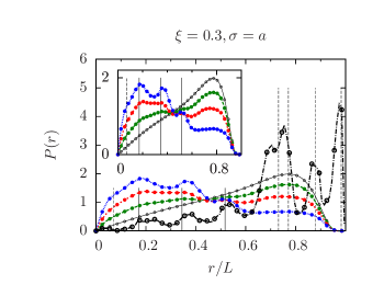
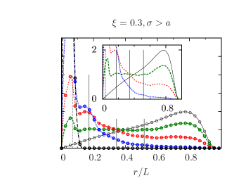
(a)	(b)

Figure 11: (Color online) End-to-end distribution for $\sigma=a$ (a) and $\sigma>a$ (b). The occupation probabilities are $p=0$ (, black), $0.64$ (, green), $0.76$ (, red),
$0.89$ (, blue), and $1$ (, black).

The impact of the disk diameter is illustrated for the example of $\xi=0.3$. Figure 11(a) shows the corresponding end-to-end distribution function for $\sigma=a$. The entropic decrease of leaving local void space leads to a stronger compression of the polymers. This is well seen in the transition of the main peak from right to left for $p=0.64,0.76,0.89$. Additionally, the undulations at small end-to-end lengths that represent crumpled configurations are more pronounced. A further difference is well seen for $p=1$. A narrower channel favors completely stretched configurations. The intersection between neighboring void spaces separated by a narrow channel acts as a new pinpoint. Having a completely occupied lattice leaves only small cavities for the polymer. For $\xi=0.3$ the length scale of the stiffness is larger than the extension of the void space. The entropic benefit provided by the larger channels for $\sigma<a$ is not given for $\sigma=a$ and thus stretched configurations contribute for a major part.

The extreme case of $\sigma>a$ such that the polymer can no longer cross between neighboring disks is illustrated in figure 11(b). Space is now separated into void-space clusters. The different contributions hence arise solely from the different clusters of void space. The fully occupied lattice finally leaves only small cavities into which the configurations are squeezed.

5.4 Leaving the constraint of a fixed pinpoint

The discussion so far was subject to the constraint of a fixed pinpoint. In this section, we compare results of a non-fixed polymer to the previous case and discuss the differences that arise. The data for the non-fixed case originate from multicanonical Monte Carlo simulations, in which the polymer may move through space by means of standard rotation and translation updates. In this case, we performed longer simulations on each disorder realization and therefore considered only $300$ of those for the quenched average. Figure 12 shows results for exemplary parameters. It can be seen that for fully occupied lattices the end-to-end distributions do not differ, as is the case for the free polymer and low disorder densities. In the high-density regime, on the other hand, the measured observables show strong differences especially in the crossover regime of $\xi=0.3$. This can be understood considering the following entropic and energetic arguments. Other than the fully occupied or the low-density case, high disorder densities produce small void spaces of different sizes which are entropically more favorable than the alternative channels. In the case of non-fixed constraints, the polymers are able to move to those small spaces and thus they contribute stronger as long as the energetic cost for bending is not too high. The results can be seen in figure 12 where the end-to-end distribution shows deviations from the case of a fixed pinpoint in the crossover regime. This effect is less pronounced for large persistence lengths, since possible gains in entropy are dominated by the cost of bending energy.

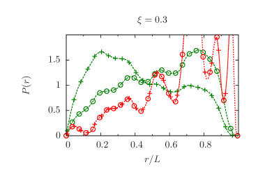
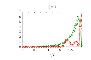
(a)	(b)

Figure 12: (Color online) End-to-end distribution function for $\xi=0.3$ (a) and $\xi=1$ (b). The occupation probabilities are: $p=0.89$ (, green), $1.00$ (, red). The data marked by $+$ are for chains that are free to move throughout space (no pinpoint) and are done by a multicanonical Monte Carlo simulation. The data marked by $\circ$ are for fixed starting point and are obtained with the growth method.

6 Conclusions

We analyzed in detail the behavior of a polymer in a potential consisting of hard disks distributed on the sites of a square lattice. We found that the polymer, depending on the ratio of persistence length and void space extension, either crumples up (small $\xi$) or straightens (large $\xi$) for increasing density of the potential. This is consistent with the results that, e.g., Cifra [14] recently found. Besides, the periodic structure of the lattice is reflected in the distribution functions of the polymer.

Furthermore, we found that the distributions—in the case of pinning the polymer at one end—strongly reflect the local cluster structure of the disorder. Leaving the constraint of pinning lets the polymer escape local cavities and gain entropy in larger void-space clusters. The corresponding distributions for pinned and non-pinned polymers differ considerably.

Finally, we checked the applicability of an off-lattice growth algorithm to the problem of a semiflexible polymer exposed to high-density disorder in the form of steric hindrance. By employing two conceptually completely different algorithms to the problem—the off-lattice growth algorithm and the multicanonical Monte Carlo method—we corroborated that the tested method is well usable. For a combination of large occupation and long persistence length the growth method is even performing better. We want to emphasize the ability of the growth algorithm to provide distributions for all chain lengths up to the desired degree of polymerization within one simulation. Equipped with this finding, a challenging next step is to investigate the behavior of semiflexible polymers in hard-disk fluid disorder.

References

References

- [1] M. E. Cates and R. C. Ball. Statistics of a polymer in a random potential, with implications for a nonlinear interfacial growth model. J. Physique, 49:2009, 1988.
- [2] Y. Y. Goldschmidt. Replica field theory for a polymer in random media. Phys. Rev. E, 61:1729, 2000.
- [3] Y. Shiferaw and Y. Y. Goldschmidt. Localization of a polymer in random media: Relation to the localization of a quantum particle. Phys. Rev. E, 63:051803, 2001.
- [4] J. Machta. Static and dynamic properties of polymers in random media. Phys. Rev. A, 40:1720, 1989.
- [5] T. Nattermann and W. Renz. Diffusion in a random catalytic environment, polymers in random media, and stochastically growing interfaces. Phys. Rev. A, 40:4675, 1989.
- [6] S. Stepanow. Polymers in a random environment. J. Phys. A, 25:6187, 1992.
- [7] G. Guillot, L. Leger, and F. Rondelez. Diffusion of large flexible polymer chains through model porous membranes. Macromolecules, 18:2531, 1985.
- [8] D. S. Cannell and F. Rondelez. Diffusion of Polystyrenes through Microporous Membranes. Macromolecules, 13:1599, 1980.
- [9] M. T. Bishop, K. H. Langley, and F. E. Karasz. Diffusion of a Flexible Polymer in a Random Porous Material. Phys. Rev. Lett. 57:1741, 1986.
- [10] A. Baumgärtner and M. Muthukumar. A trapped polymer chain in random porous media. J. Chem. Phys., 87:3082, 1987.
- [11] S. Schöbl, J. Zierenberg, and W. Janke. Simulating flexible polymers in a potential of randomly distributed hard disks. Phys. Rev. E, 84:051805, 2011.
- [12] H. Hinsch and E. Frey. Conformations of entangled semiflexible polymers: Entropic trapping and transient non-equilibrium distributions. ChemPhysChem, 10:2891, 2009.
- [13] A. Dua and T. A. Vilgis. Semiflexible polymers in a random environment. J. Chem. Phys., 121:5505, 2004.
- [14] P. Cifra. Weak-to-strong confinement transition of semi-flexible macromolecules in slit and in channel. J. Chem. Phys., 136:024902, 2012.
- [15] C. J. Thompson. Classical Equilibrium Statistical Mechanics. Oxford University Press, Oxford, UK, 1988.
- [16] O. Kratky and G. Porod. X-ray investigation of dissolved chain molecules. Rec. Trav. Chim. Pays-Bas., 68:1106, 1949.
- [17] M. Doi and S. F. Edwards. The Theory of Polymer Dynamics. Oxford University Press, Walton Street, Oxford, UK, 1986.
- [18] M. Abramowitz and A. I. Stegun. Handbook of Mathematical Functions. Dover Publications, New York, US, 1965.
- [19] L. D. Landau and E. M. Lifshitz. Theory of Elasticity. Pergamon Press, Oxford, UK, 1959.
- [20] D. Stauffer and A. Aharony. Introduction to Percolation Theory. Taylor and Francis, London, 1992.
- [21] T. Garel and H. Orland. Guided replication of random chains: a new Monte Carlo method. J. Phys. A, 23:L621, 1990.
- [22] B. A. Berg and T. Neuhaus. Multicanonical algorithms for first order phase transitions. Phys. Lett. B, 267:249, 1991.
- [23] B. A. Berg and T. Neuhaus. Multicanonical ensemble: A new approach to simulate first-order phase transitions. Phys. Rev. Lett., 68:9, 1992.
- [24] W. Janke. Multicanonical Monte Carlo simulations. Physica A, 254:164, 1998.
- [25] W. Janke. Statistical analysis of simulations: data correlations and error estimation. Quantum Simulations of Complex Many-Body Systems: From Theory to Algorithms eds J. Grotendorst, D. Marx and A. Muramatsu. NIC Series (Jülich: Forschungszentrum Jülich Press), 10:423, 2002.
- [26] P. G. Higgs and H. Orland. Scaling behavior of polyelectrolytes and polyampholytes: Simulation by an ensemble growth method. J. Chem. Phys., 95:4506, 1991.
- [27] J. Wilhelm and E. Frey. Radial distribution function of semiflexible polymers. Phys. Rev. Lett., 77:2581, 1996.
- [28] B. Hamprecht, W. Janke, and H. Kleinert. End-to-end distribution function of two-dimensional stiff polymers for all persistence lengths. Phys. Lett. A, 330:254, 2004.
- [29] M. Rubinstein and R. H. Colby. Polymer Physics. Oxford University Press, Oxford, UK, 2003.
- [30] H.-P. Hsu, W. Paul, and K. Binder. Polymer chain stiffness vs. excluded volume: A Monte Carlo study of the crossover towards the worm-like chain model. Europhys. Lett., 92:28003, 2010.
- [31] Hsu H.-P., W. Paul, and K. Binder. Breakdown of the Kratky-Porod wormlike chain model for semiflexible polymers in two dimensions. Europhys. Lett., 95:68004, 2011.
- [32] K. Kroy and J. Glaser. The glassy wormlike chain. New Journal of Physics, 9:416, 2007.
- [33] V. Yamakov and A. Milchev. Diffusion of a polymer chain in porous media. Phys. Rev. E, 55:1704, 1997.
- [34] C. Echeverria and R. Kapral. Macromolecular dynamics in crowded environments. J. Chem. Phys., 132:104902, 2010.