Some principles for mountain pass algorithms, and the parallel distance

Abstract.

The problem of computing saddle points is important in certain problems in numerical partial differential equations and computational chemistry, and is often solved numerically by a minimization problem over a set of mountain passes. We point out that a good global mountain pass algorithm should have good local and global properties. Next, we define the parallel distance, and show that the square of the parallel distance has a quadratic property. We show how to design algorithms for the mountain pass problem based on perturbing parameters of the parallel distance, and that methods based on the parallel distance have midrange local and global properties.

1. Introduction

We begin with the definition of a mountain pass.

Definition 1.1.

(Mountain pass) Let $X$ be a topological space, and consider $a,b\in X$. Let $\Gamma(a,b)$ be the set of continuous paths $p:[0,1]\rightarrow X$ such that $p(0)=a$ and $p(1)=b$. For a function $f:X\rightarrow\mathbb{R}$, define an optimal mountain pass $\bar{p}\in\Gamma(a,b)$ to be a minimizer of the problem

$$\inf_{p\in\Gamma(a,b)}\sup_{0\leq t\leq 1}f\circ p(t).$$ (1.1)

The point $\bar{x}$ is a critical point if $\nabla f(\bar{x})=0$, and the critical point $\bar{x}$ is a saddle point if it is not a local maximizer or minimizer on $X$. The value $f(x)$ is a critical value if $x$ is a critical point. We say that $\bar{x}$ is a saddle point of mountain pass type if there is an open set $U$ containing $\bar{x}$ such that $\bar{x}$ lies in the closure of two path connected components of $\{x\in U:f(x)<f(\bar{x})\}$. In the case where $f$ is smooth and an optimal mountain pass $\bar{p}:[0,1]\to X$ exists, the maximum of $f$ on $\bar{p}([0,1])$ is a saddle point.

In this paper, we shall focus on the case where $X=\mathbb{R}^{n}$ and the saddle point is nondegenerate. A saddle point $\bar{x}$ is said to be nondegenerate if $\nabla^{2}f(\bar{x})$ is invertible. Moreover, a nondegenerate saddle point $\bar{x}$ has Morse index one if $\nabla^{2}f(\bar{x})$ contains exactly one negative eigenvalue.

The problem of finding saddle points numerically is important in the problem of finding weak solutions to partial differential equations numerically. The first critical point existence theorems now known as the mountain pass theorems were proved in [AR73, Rab77]. Some recent theoretical references include [MW89, Rab86, Sch99, Str08, Wil96]. See also the more accessible reference [Jab03]. The original paper of a mountain pass algorithm to solve partial differential equations is [CM93], and it contains several semilinear elliptic problems. Particular applications in numerical partial differential equations include finding periodic solutions of a boundary value problem modeling a suspension bridge [Fen94] (introduced by [LM91]), studying a system of Ginzburg-Landau type equations arising in the thin film model of superconductivity [GM08], the choreographical 3-body problem [ABT06], and cylinder buckling [HLP06]. Other notable works in computing saddle points for solving numerical partial differential equations include the use of constrained optimization [Hor04], extending the mountain pass algorithm to find saddle points of higher Morse index [DCC99, LZ01], extending the mountain pass algorithm to find nonsmooth saddle points [YZ05], and using symmetry [WZ04, WZ05].

The problem of finding saddle points numerically is by now well entrenched in the chemistry curriculum. In transition state theory, the problem of finding the least amount of energy to transition between two stable states is equivalent to finding an optimal mountain pass between these two stable states. The highest point on the optimal mountain pass can then be used to determine the reaction kinetics. The foundations of transition state theory was laid by Marcelin, and important work by Eyring and Polanyi in 1931 and by Pelzer and Wigner a year later established the importance of saddle points in transition state theory. We cite the Wikipedia entry on transition state theory for more on its history and further references. Numerous methods for computing saddle points were suggested through the years, and we refer to the surveys [HJJ00, HS05, Sch11, Wal06] as well as the recent text [Wal03]. A software for computing saddle points in chemistry is Gaussian. Tools for computing transition states are also included in VASP. Though the entire optimal mountain pass is needed for such an application, the process of computing saddle points often gives hints on an optimal mountain pass.

As mentioned in [LP11], our initial interest in the problem of computing saddle points of mountain pass type comes from computing the distance of a matrix $A\in\mathbb{C}^{n\times n}$ to the closest matrix with repeated eigenvalues (also known as the Wilkinson distance problem).

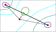
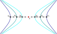
Figure 1.1. The diagram on the left illustrates a path-based method, while the diagram on the right illustrates a level set method, as was done in [LP11] and this paper.

We recall three broad methods for computing the mountain pass:

Path-based methods

The typical mountain pass algorithm makes use of the formula in (1.1) to find a saddle point. The paths in $\Gamma(a,b)$ are discretized, and perturbed so that the maximum value of $f$ along the path is reduced. The point on an optimizing path attaining the maximum value is a good estimate of the critical point. See Figure 1.1.

Quadratic model methods

Once the iterates are close enough to the saddle point $\bar{x}$, the quadratic expansion

$$f(x)=\frac{1}{2}(x-\bar{x})^{T}\nabla^{2}f(\bar{x})(x-\bar{x})+\nabla f(\bar{x})^{T}(x-\bar{x})+f(\bar{x})+o(\|x-\bar{x}\|^{2})$$ (1.2)

can form the basis of algorithms that converge quickly to the saddle point. A Newton method can achieve quadratic convergence to the saddle point, or its variants can achieve fast convergence. The gradient $\nabla f(x)$ has close to linear behavior, and other methods involving solving the linear system are also possible.

Level set methods

In [LP11, MF01], a different strategy of using level sets

$$\mbox{\rm lev}_{\leq l}f:=\{x:f(x)\leq l\}$$

is suggested: For a neighborhood $U$ of the critical point $\bar{x}$ and an increasing sequence of $l_{i}$ converging to the critical value $f(\bar{x})$, find the closest points in different components of $U\cap\mbox{\rm lev}_{\leq l_{i}}f$, say $x_{i}$ and $y_{i}$. Figure 1.1 contrasts path-based methods and level set methods. Under additional conditions, $\{x_{i}\}_{i=1}^{\infty}$ and $\{y_{i}\}_{i=1}^{\infty}$ both converge to $\bar{x}$. An optimal mountain pass can be estimated from the iterates $\{x_{i}\}_{i=1}^{\infty}$ and $\{y_{i}\}_{i=1}^{\infty}$. Advantages of level set methods over path-based methods include:

• The level set method needs only to keep track of two points at each step instead of an entire path.

• The bulk of computations are performed near the saddle point.

• The distance between the components of the level set indicate the performance of the algorithm.

• Provided black boxes for finding closest points to components of the level set and for the minimization of the function $f$ on an affine space exist, an algorithm locally superlinearly convergent to the critical point is described in [LP11]. See also (D1) in Section 3.

However, here are some difficulties encountered in the level set algorithm in [LP11], which we will elaborate in Section 3.

One contribution we make in this paper is to identify properties desirable for a global mountain pass algorithm. Specifically, we propose these two principles:

1. Suppose $f\in\mathcal{C}^{2}$. Once the iterates are close enough to a nondegenerate saddle point of Morse index one, the algorithm should converge quickly to the saddle point $\bar{x}$.

2. The global algorithm should find a saddle point of mountain pass type.

The analogy to Principle (P2) in optimization is to seek decrease so that iterates converge to a local minimizer. Principle (P1) states that the algorithm should have fast convergence once close enough to a saddle point. Related to Principle (P1) is Principle (P1^′) below.

1. For the quadratic $f(x)=\frac{1}{2}x^{T}Hx+g^{T}x+c$, where $H$ is an invertible symmetric matrix with one negative eigenvalue and $n-1$ positive eigenvalues, the algorithm should have excellent convergence.

We make a short summary of the performance of the various mountain pass algorithms. Path-based methods excel in (P2) due to the proof of the mountain pass theorem of [AR73] using the Ekeland variational principle. More specifically, under suitable conditions, if $p_{i}(\cdot)$ is a sequence of paths in $\Gamma(a,b)$ such that $\max_{t\in[0,1]}f\circ p_{i}$ converges to the critical level, then the sequence of maximizers of $f$ along the path $p_{i}(\cdot)$ converge to a saddle point. However, it does poorly for (P1) and (P1^′) because it does not take advantage of the quadratic approximation (1.2) to achieve fast convergence. On the other hand, methods that make extensive use of the quadratic approximation (1.2) excel for (P1) and (P1^′), but does not satisfy (P2) because the quadratic approximation need not be valid globally.

Another contribution of this paper is to argue that level set methods should be part of a good mountain pass algorithm because it does well for the Principles (P1), (P1^′) and (P2).

We also show how the parallel distance defined below can be part of a good mountain pass algorithm. For a set $C\subset\mathbb{R}^{n}$, its diameter $\mbox{\rm diam}(C)$ is defined by $\mbox{\rm diam}(C):=\sup\{|x-y|:x,y\in C\}$.

Definition 1.2.

(Parallel distance) Let $f:\mathbb{R}^{n}\to\mathbb{R}$ be $\mathcal{C}^{2}$ in a convex neighborhood $U^{\prime}$, and let $v$ be a unit vector. See Figure 1.2. Consider the set $S_{l,v}(x)\subset\mathbb{R}^{n}$ defined by

$$S_{l,v}(x):=U^{\prime}\cap[\{x\}+\mathbb{R}\{v\}]\cap\mbox{\rm lev}_{\geq l}f.$$

For a neighborhood $U$ of $\bar{x}$ such that $U\subset U^{\prime}$, define the parallel distance $g_{l,v}:U\to\mathbb{R}$ by

$$g_{l,v}(x):=\mbox{\rm diam}\big{(}S_{l,v}(x)\big{)}.$$

When $S_{l,v}(x)=\emptyset$, $g_{l,v}(x)=0$. In the case where $S_{l,v}(x)$ is a line segment, we can write $g_{l,v}(x)$ as

$$g_{l,v}(x)=g_{l,v,1}(x)+g_{l,v,2}(x),$$ (1.3)

where

$$g_{l,v,1}(x) = \max\{\phantom{-}v^{T}z^{\phantom{\prime}}\mid f(z^{\phantom{\prime}})=l,\,z^{\phantom{\prime}}\in S_{l,v}(x)\},$$ (1.4a)

$$\mbox{ and }g_{l,v,2}(x) = \max\{-v^{T}z^{\prime}\mid f(z^{\prime})=l,\,z^{\prime}\in S_{l,v}(x)\}.$$ (1.4b)

Also, define $z(x)$ and $z^{\prime}(x)$ as

$$z^{\phantom{\prime}}(x) = \arg\max\{\phantom{-}v^{T}z^{\phantom{\prime}}\mid f(z^{\phantom{\prime}})=l,\,z^{\phantom{\prime}}\in S_{l,v}(x)\},$$

$$\mbox{ and }z^{\prime}(x) = \arg\max\{-v^{T}z^{\prime}\mid f(z^{\prime})=l,\,z^{\prime}\in S_{l,v}(x)\}.$$

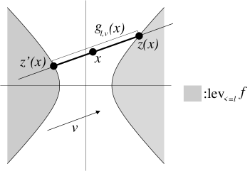
Figure 1.2. Illustration of $g_{l,v}(x)$ in Definition 1.2.

One step of the mountain pass algorithm in [LP11] is to find the closest points between components of the level sets. The problem of finding the closest points between two sets is not necessarily easy, and an alternating projection algorithm converges slowly once close to the optimum points. We will show that as long as $v$ is close enough to the eigenvector corresponding to the negative eigenvalue of the Hessian of the saddle point, the square of the parallel distance satisfies property (P1). This allows us to get around the problem of finding the closest points between components of the level sets.

1.1. Outline of paper

Section 2 discusses various basic properties of the parallel distance. The topics discussed are: how the square of the parallel distance satisfies (P1^′), formulas for the gradient and Hessian of the parallel distance $g_{l,v}(\cdot)$ and its square $g_{l,v}(\cdot)^{2}$, and why it is preferable to consider $g_{l,v}(\cdot)^{2}$ for the smooth problem instead of $g_{l,v}(\cdot)$. Section 3 proposes subroutines for a mountain pass algorithm, and discusses how to use these subroutines to design a mountain pass algorithm with midrange local and global properies. Section 4 shows that the Hessian $\nabla^{2}(g_{l,v}^{2})(\cdot)$ is close to the Hessian as predicted by a quadratic model. This shows that the Hessian $\nabla^{2}(g_{l,v}^{2})(\cdot)$ is not sensitive to $l$ as the computations get close to the saddle point, making old estimates of $\nabla^{2}(g_{l,v}^{2})(\cdot)$ useful for future computations involving a different $l$. Section 5 shows how our algorithm performs in an implementation.

2. Basic properties of the parallel distance

In this section, we study basic properties of the parallel distance function.

When $f$ is an exact quadratic whose critical point is nondegenerate of Morse index one, we have the following appealing result.

Proposition 2.1.

(Quadratic formula for square of parallel distance in exact quadratic) Suppose that $f:\mathbb{R}^{n}\to\mathbb{R}$ is an exact quadratic $f(x)=\frac{1}{2}x^{T}Hx+g^{T}x+c$, with $H\in\mathbb{R}^{n\times n}$ having $n-1$ positive eigenvalues and one negative eigenvalue. Consider a unit vector $v$ such that $v^{T}Hv<0$. Then $S_{l,v}(x)$ is a line segment, and the function $g_{l,v}(\cdot)$ takes the form (1.3). Additionally, we have

$$g_{l,v}(x)^{2} =\max\Big{\{}0,\frac{4}{(v^{T}Hv)^{2}}\Big{[}x^{T}[Hvv^{T}H-(v^{T}Hv)H]x$$

$$\qquad\qquad\qquad\qquad\qquad+2[(g^{T}v)v^{T}H-(v^{T}Hv)g^{T}]x$$

$$\qquad\qquad\qquad\qquad\qquad+\big{[}(g^{T}v)^{2}+(v^{T}Hv)[-2c+2l]\big{]}\Big{]}\Big{\}}.$$ (2.1)

For $g_{l,v}(x)>0$ and $v$ sufficiently close to the eigenvector corresponding to the negative eigenvalue of $H$, the matrix $\nabla^{2}(g_{l,v}^{2})(x)$ has $n-1$ positive eigenvalues and one zero eigenvalue. The function $g_{l,v}^{2}$ is convex. Moreover, let $\bar{x}$ be the saddle point $-H^{-1}g$. If $l<f(\bar{x})$ and $g_{l,v}^{2}$ has a minimizer $\tilde{x}$, then $\bar{x}$ is the midpoint of the intersection of the line $\{\tilde{x}\}+\mathbb{R}\{v\}$ and $\mbox{\rm lev}_{=l}f$.

Proof.

For the case of the quadratic $f$, the neighborhoods $U$ and $U^{\prime}$ can be taken to be $\mathbb{R}^{n}$. The value $g_{l,v}(x)$ can be computed as follows. At where $g_{l,v}(x)>0$, let $x+t_{i}v$, where $t_{i}\in\mathbb{R}$ and $i=1,2$, be two points of intersection of the line $\{x\}+\mathbb{R}\{v\}$ and the curve $\mbox{\rm lev}_{=l}f$. The $t_{i}$’s can be calculated as follows:

$$\frac{1}{2}(x+t_{i}v)^{T}H(x+t_{i}v)+g^{T}(x+t_{i}v)+c = l$$

$$\Rightarrow(v^{T}Hv)t_{i}^{2}+[2(v^{T}Hx)+2g^{T}v]t_{i}+x^{T}Hx+2g^{T}x+2c-2l = 0.$$

We have

$$t_{i}=\frac{-2(v^{T}Hx)-2g^{T}v\pm\sqrt{4(v^{T}Hx+g^{T}v)^{2}-4(v^{T}Hv)(x^{T}Hx+2g^{T}x+2c-2l)}}{2(v^{T}Hv)}.$$

This gives

$$g_{l,v}(x) = \frac{2}{v^{T}Hv}\sqrt{(v^{T}Hx+g^{T}v)^{2}-(v^{T}Hv)(x^{T}Hx+2g^{T}x+2c-2l)}$$

$$g_{l,v}(x)^{2} = \frac{4}{(v^{T}Hv)^{2}}[(v^{T}Hx+g^{T}v)^{2}-(v^{T}Hv)(x^{T}Hx+2g^{T}x+2c-2l)]$$

$$= \frac{4}{(v^{T}Hv)^{2}}\Big{[}x^{T}[Hvv^{T}H-(v^{T}Hv)H]x+2[(g^{T}v)v^{T}H-(v^{T}Hv)g^{T}]x$$

$$\qquad\qquad\qquad+\big{[}(g^{T}v)^{2}+(v^{T}Hv)[-2c+2l]\big{]}\Big{]}.$$

Taking into account the fact that $g_{l,v}(x)$ can equal zero, $g_{l,v}(x)^{2}$ has the formula as given in (2.1). For the case when $v=\bar{v}$, the eigenvector corresponding to the negative eigenvalue of $H$, we find that $\bar{v}$ is the eigenvector corresponding the zero eigenvalue for the Hessian

$$\nabla^{2}(g_{l,\bar{v}}^{2})(x)=\frac{8}{(v^{T}Hv)^{2}}[Hvv^{T}H-(v^{T}Hv)H].$$

The other eigenvalues of $\nabla^{2}(g_{l,\bar{v}}^{2})(x)$ can easily be calculated to be $-8\lambda_{i}/\lambda_{n}$ for $i=1,\dots,n-1$, where $\lambda_{i}$s are the eigenvalues of $H$ arranged in decreasing order.

Note that $v$ is an eigenvector corresponding to eigenvalue zero of $\nabla^{2}(g_{l,v}^{2})(x)$. Recall that the eigenvalues depend continuously on the matrix entries. If the unit vector $v$ is sufficiently close to $\bar{v}$, then the Hessian $\nabla^{2}(g_{l,v}^{2})(x)$ has one zero eigenvalue and $n-1$ positive eigenvalues. The convexity of $g_{l,v}^{2}(\cdot)$ is clear.

In the case where $l<f(\bar{x})$, it is easy to check that $x=-H^{-1}g$ is a minimizer of $g_{l,v}^{2}(\cdot)$. The other claims are easy. ∎

Proposition 2.1 says that when $f$ is quadratic, then $g_{l,v}(\cdot)^{2}$ is also a quadratic, so a mountain pass algorithm based on the parallel distance will satisfy (P1^′).

We next show that the parallel distance behaves well near the saddle point $\bar{x}$ of Morse index one.

Proposition 2.2.

(Behavior near saddle point) Let $f:\mathbb{R}^{n}\to\mathbb{R}$ be $\mathcal{C}^{2}$ in a neighborhood of a nondegenerate saddle point $\bar{x}$ of Morse index one, and $\bar{v}$ be the eigenvector of unit length corresponding to the negative eigenvector of $\nabla^{2}f(\bar{x})$. For $\delta>0$, define $\bar{f}_{\delta}:\mathbb{R}^{n}\to\mathbb{R}$ and $\bar{S}_{\delta,l,v}(x)$ by

$$\bar{f}_{\delta}(x) := \frac{1}{2}(x-\bar{x})^{T}[\nabla^{2}f(\bar{x})+\delta I](x-\bar{x})+f(\bar{x}),$$ (2.2)

$$\mbox{ and }\bar{S}_{\delta,l,v}(x) := [\{x\}+\mathbb{R}\{v\}]\cap\mbox{\rm lev}_{\geq l}\bar{f}_{\delta}.$$

There is a neighborhood $U^{\prime}$ of $\bar{x}$ and $\epsilon>0$ such that:

1. $\|\nabla^{2}f(\bar{x})-\nabla^{2}f(x)\|<\delta$ for all $x\in U^{\prime}$.

2. If $\|v-\bar{v}\|<\epsilon$, then the map $t\mapsto f(x+tv)$, where $t\in\mathbb{R}$, is concave at wherever $x+tv\in U^{\prime}$. Hence $S_{l,v}(x)$ is either a line segment or an empty set.

3. If $v$ is a unit vector satisfying $\|v-\bar{v}\|<\epsilon$ and $|l-f(\bar{x})|<\epsilon$, then for all $x\in\mathbb{B}_{\epsilon}(\bar{x})$, we have $S_{l,v}(x)\cap U^{\prime}\subset\bar{S}_{\delta,l,v}(x)\subset U^{\prime}$ (which includes the case $S_{l,v}(x)=\emptyset$).

Proof.

The statement (1) holds for some $U^{\prime}$ of $\bar{x}$. We can shrink $U^{\prime}$ if necessary so that $\bar{v}^{T}\nabla^{2}f(x)\bar{v}<0$ for all $x\in U^{\prime}$, and an $\epsilon>0$ can be found so that (2) is satisfied.

Choose $\gamma>0$ such that $\mathbb{B}_{\gamma}(\bar{x})\subset U^{\prime}$. Then condition (1) ensures that $f(x)<\bar{f}_{\delta}(x)$ for all $x\in U^{\prime}$, so $S_{l,v}(x)\cap U^{\prime}\subset\bar{S}_{\delta,l,v}(x)$. The endpoints of the line segment $\bar{S}_{l,v}(x)$ are of the form $[x+\tilde{t}_{1}v,x+\tilde{t}_{2}v]$, whose endpoints can be calculated using the quadratic formula employed in the proof of Proposition 2.1 as $x+\tilde{t}_{i}v$, $i=1,2$, giving us

$$\tilde{t}_{i} = -\frac{[v^{T}H_{\delta}(x-\bar{x})]}{v^{T}H_{\delta}v}$$

$$\pm\frac{\sqrt{4[v^{T}H_{\delta}(x-\bar{x})]^{2}-4[v^{T}H_{\delta}v][(x-\bar{x})^{T}H_{\delta}(x-\bar{x})+2f(\bar{x})-2l]}}{2[v^{T}H_{\delta}v]},$$

where $H_{\delta}=\nabla^{2}f(\bar{x})+\delta I$. The formula above is continuous in $v$, $x$ and $l$ whenever $\tilde{t}_{i}$ is real, and as $x\to\bar{x}$ and $l\to f(\bar{x})$, we have $\tilde{t}_{i}\to 0$. From $\|x+\tilde{t}_{i}v-\bar{x}\|\leq\|x-\bar{x}\|+|\tilde{t}_{i}|$, we can choose $\epsilon$ small enough so that if $\|v-\bar{v}\|<\epsilon$, $|l-f(\bar{x})|<\epsilon$ and $x\in\mathbb{B}_{\epsilon}(\bar{x})$, then $\|x+\tilde{t}_{i}v-\bar{x}\|<\gamma$, giving us $\bar{S}_{\delta,l,v}(x)\subset\mathbb{B}_{\gamma}(\bar{x})\subset U^{\prime}$. This means that condition (3) holds. ∎

The expression (1.3) gives us a way to calculate derivatives of the parallel distance. We have the following results.

Lemma 2.3.

(Gradient and Hessian of $g_{l,v}$) Let $f:\mathbb{R}^{n}\to\mathbb{R}$ be $\mathcal{C}^{2}$ everywhere. Recall the function $g_{l,v}:\mathbb{R}^{n}\to\mathbb{R}$ and the neighborhoods $U$ and $U^{\prime}$ on which $g_{l,v}$ is defined. Suppose that $g_{l,v}$ can be represented as (1.3). Let $z(x)$ and $z^{\prime}(x)$ be the respective maximizers in the definitions of $g_{l,v,1}$ and $g_{l,v,2}$ in (1.4a) and (1.4b). Then, provided $\nabla f(z(x))^{T}v\neq 0$ and $\nabla f(z^{\prime}(x))^{T}v\neq 0$, we have

$$\nabla g_{l,v}(x)=-\frac{\nabla f(z(x))}{\nabla f(z(x))^{T}v}+\frac{\nabla f(z^{\prime}(x))}{\nabla f(z^{\prime}(x))^{T}v}.$$

To simplify the notation, we suppress the dependence of $z$ and $z^{\prime}$ on $x$. We also have

$$\nabla^{2}g_{l,v}(x) = -\left(I-\frac{\nabla f(z)v^{T}}{v^{T}\nabla f(z)}\right)\frac{\nabla^{2}f(z)}{v^{T}\nabla f(z)}\left(I-\frac{\nabla f(z)v^{T}}{v^{T}\nabla f(z)}\right)^{T}$$

$$+\left(I-\frac{\nabla f(z^{\prime})v^{T}}{v^{T}\nabla f(z^{\prime})}\right)\frac{\nabla^{2}f(z^{\prime})}{v^{T}\nabla f(z^{\prime})}\left(I-\frac{\nabla f(z^{\prime})v^{T}}{v^{T}\nabla f(z^{\prime})}\right)^{T}.$$

Proof.

Write $F(d,t):=f(x+tv+d)=f\big{(}(x+\bar{t}v)+d+(t-\bar{t})v\big{)}$. We evaluate the partial derivatives of $F$ at $(0,\bar{t})$ to be

$$\nabla_{d}F(0,\bar{t})=\nabla f(x+\bar{t}v)\qquad\mbox{and}\qquad\nabla_{t}F(0,\bar{t})=\nabla f(x+\bar{t}v)^{T}v.$$

For each $d$, we can find $t$ such that $F(d,t)=0$. By the implicit function theorem, the derivative of $t$ with respect to $d$ equals $-\frac{\nabla f(x+\bar{t}v)}{\nabla f(x+\bar{t}v)^{T}v}=-\frac{\nabla f(z(x))}{\nabla f(z(x))^{T}v}$ provided the denominator is nonzero. From this and the fact that $g_{l,v,1}(\cdot)$ and $g_{l,v,2}(\cdot)$ are constant when moving in the direction $v$, we get

$$\nabla g_{l,v,1}(x)=-\frac{\nabla f(z(x))}{\nabla f(z(x))^{T}v}+v.$$ (2.3)

Similarly, we have $\nabla g_{l,v,2}(x)=\frac{\nabla f(z^{\prime}(x))}{\nabla f(z^{\prime}(x))^{T}v}-v$. The formula for $\nabla g_{l,v}$ is easily deduced.

Next, we calculate $\nabla^{2}g_{l,v}$ by first calculating $\nabla^{2}g_{l,v,1}$ and $\nabla^{2}g_{l,v,2}$. To reduce notation, we suppress the dependence of $z$ and $z^{\prime}$ on $x$. Taking the $m$th component of (2.3) gives

$$\frac{\partial g_{l,v,1}}{\partial x_{m}}(x)=-\frac{1}{v^{T}\nabla f(z)}\frac{\partial f(z)}{\partial x_{m}}+v_{m},$$

so

$$\frac{\partial}{\partial x_{m^{\prime}}}\left(\frac{\partial g_{l,v,1}}{\partial x_{m}}\right)(x) = \frac{-[v^{T}\nabla f(z)]\frac{\partial}{\partial x_{m^{\prime}}}\left(\frac{\partial f(z)}{\partial x_{m}}\right)+\frac{\partial f(z)}{\partial x_{m}}\left[\frac{\partial}{\partial x_{m^{\prime}}}(v^{T}\nabla f(z))\right]}{[v^{T}\nabla f(z)]^{2}}.$$

Note that $z(x)=x+g_{l,v,1}(x)v-vv^{T}x$ and $z^{\prime}(x)=x-g_{l,v,2}(x)v+vv^{T}x$. We use the notation $1_{\{a=b\}}$ to mean

$$1_{\{a=b\}}=\begin{cases}1&\mbox{ if }a=b\\ 0&\mbox{ otherwise.}\end{cases}$$

So $\frac{\partial z_{k}}{\partial x_{m^{\prime}}}=1_{\{m^{\prime}=k\}}+\frac{\partial g_{l,v,1}(x)}{\partial x_{m^{\prime}}}v_{k}-v_{m^{\prime}}v_{k}$, and $\frac{\partial z^{\prime}_{k}}{\partial x_{m^{\prime}}}=1_{\{m^{\prime}=k\}}-\frac{\partial g_{l,v,2}(x)}{\partial x_{m^{\prime}}}v_{k}+v_{m^{\prime}}v_{k}.$ So by the multi-variable chain rule we have

$$\frac{\partial}{\partial x_{m^{\prime}}}\left(\frac{\partial g_{l,v,1}}{\partial x_{m}}\right)(x)$$

$$= \frac{-[v^{T}\nabla f(z)]\sum_{k=1}^{n}\left[\frac{\partial^{2}f(z)}{\partial x_{k}\partial x_{m}}\left[1_{\{m^{\prime}=k\}}+\frac{\partial g_{l,v,1}(x)}{\partial x_{m^{\prime}}}v_{k}-v_{m^{\prime}}v_{k}\right]\right]}{[v^{T}\nabla f(z)]^{2}}$$

$$+\frac{\frac{\partial f(z)}{\partial x_{m}}\sum_{k=1}^{n}\left[v_{k}\sum_{k^{\prime}=1}^{n}\frac{\partial^{2}f(z)}{\partial x_{k}\partial x_{k^{\prime}}}\left[1_{\{k^{\prime}=m^{\prime}\}}+\frac{\partial g_{l,v,1}(x)}{\partial x_{m^{\prime}}}v_{k^{\prime}}-v_{m^{\prime}}v_{k^{\prime}}\right]\right]}{[v^{T}\nabla f(z)]^{2}}.$$

Now we have,

$$\nabla^{2}g_{l,v,1}(x) = \frac{-\nabla^{2}f(z)-\nabla^{2}f(z)v[\nabla g_{l,v,1}(x)^{T}-v^{T}]}{v^{T}\nabla f(z)}$$

$$+\frac{\nabla f(z)v^{T}\nabla^{2}f(z)+\nabla f(z)v^{T}\nabla^{2}f(z)v[\nabla g_{l,v,1}(x)^{T}-v^{T}]}{[v^{T}\nabla f(z)]^{2}}.$$

Substituting $\nabla g_{l,v,1}(x)=-\frac{\nabla f(z)}{v^{T}\nabla f(z)}+v$, we get:

$$\nabla^{2}g_{l,v,1}(x)$$

$$= -\frac{\nabla^{2}f(z)}{v^{T}\nabla f(z)}+\frac{\nabla^{2}f(z)v\nabla f(z)^{T}+\nabla f(z)v^{T}\nabla^{2}f(z)}{[v^{T}\nabla f(z)]^{2}}$$

$$-\frac{\nabla f(z)v^{T}\nabla^{2}f(z)v\nabla f(z)^{T}}{[v^{T}\nabla f(z)]^{3}}.$$

The formula for $\nabla^{2}g_{l,v,2}(x)$ is similar, and the formula for $\nabla^{2}g_{l,v}(x)$ follows readily. ∎

The formulas for $\nabla(g_{l,v}^{2})$ and $\nabla^{2}(g_{l,v}^{2})$ can now be calculated, as is done below.

Proposition 2.4.

(Gradient and Hessian of $g_{l,v}^{2}$) Given the conditions in Lemma 2.3, the formulas for $\nabla(g_{l,v}^{2})(x)$ and $\nabla^{2}(g_{l,v}^{2})(x)$ are $\nabla(g_{l,v}^{2})(x)=2g_{l,v}(x)\nabla g_{l,v}(x)$ and

$$\nabla^{2}(g_{l,v}^{2})(x) = 2\left(-\frac{\nabla f(z)}{\nabla f(z)^{T}v}+\frac{\nabla f(z^{\prime})}{\nabla f(z^{\prime})^{T}v}\right)\left(-\frac{\nabla f(z)}{\nabla f(z)^{T}v}+\frac{\nabla f(z^{\prime})}{\nabla f(z^{\prime})^{T}v}\right)^{T}$$

$$-2g_{l,v}(x)\left(I-\frac{\nabla f(z)v^{T}}{v^{T}\nabla f(z)}\right)\frac{\nabla^{2}f(z)}{v^{T}\nabla f(z)}\left(I-\frac{\nabla f(z)v^{T}}{v^{T}\nabla f(z)}\right)^{T}$$

$$+2g_{l,v}(x)\left(I-\frac{\nabla f(z^{\prime})v^{T}}{v^{T}\nabla f(z^{\prime})}\right)\frac{\nabla^{2}f(z^{\prime})}{v^{T}\nabla f(z^{\prime})}\left(I-\frac{\nabla f(z^{\prime})v^{T}}{v^{T}\nabla f(z^{\prime})}\right)^{T}.$$

Proof.

We have $\frac{\partial(g_{l,v}^{2})}{\partial x_{m}}(x)=2g_{l,v}(x)\frac{\partial(g_{l,v})}{\partial x_{m}}(x)$, so $\nabla(g_{l,v}^{2})(x)=2g_{l,v}(x)\nabla g_{l,v}(x)$. Also,

$$\frac{\partial}{\partial x_{m^{\prime}}}\left(\frac{\partial(g_{l,v}^{2})}{\partial x_{m}}(x)\right)=2\frac{\partial g_{l,v}(x)}{\partial x_{m^{\prime}}}\frac{\partial g_{l,v}(x)}{\partial x_{m}}+2g_{l,v}(x)\frac{\partial^{2}g_{l,v}(x)}{\partial x_{m^{\prime}}\partial x_{m}}.$$

We thus have

$$\nabla^{2}(g_{l,v}^{2})(x)=2\nabla g_{l,v}(x)\nabla g_{l,v}(x)^{T}+2g_{l,v}(x)\nabla^{2}g_{l,v}(x),$$

which gives the formula for $\nabla^{2}(g_{l,v}^{2})(x)$. ∎

We now discuss the situation when we consider $g_{l,v}$ instead of its square. Consider a quadratic function $f:\mathbb{R}^{n}\to\mathbb{R}$ whose Hessian has one negative eigenvalue and $n-1$ positive eigenvalues. For the critical point $\bar{x}$ and critical level $f(\bar{x})$, a plot of $\mbox{\rm lev}_{\leq l}f$ for $l<f(\bar{x})$ has two distinct convex components. One would expect that if $f:\mathbb{R}^{n}\to\mathbb{R}$ is $\mathcal{C}^{2}$ at a nondegenerate saddle point $\bar{x}$ of Morse index one and $l<f(\bar{x})$, $U\cap\mbox{\rm lev}_{\leq l}f$ would consist of two convex components for some neighborhood $U$ of $\bar{x}$. We have the following result on the convexity of the level sets from [LP11].

Proposition 2.5.

[LP11] (Convexity of level sets) Suppose that $f:\mathbb{R}^{n}\rightarrow\mathbb{R}$ is $\mathcal{C}^{2}$ in a neighborhood of a nondegenerate critical point $\bar{x}$ of Morse index one. Then if $\epsilon>0$ is small enough, there is a convex neighborhood $U_{\epsilon}$ of $\bar{x}$ such that $U_{\epsilon}\cap\mbox{\rm lev}_{\leq f(\bar{x})-\epsilon}f$ is a union of two disjoint convex sets.

The example below show that Proposition 2.5 may be the best possible.

Example 2.6.

(Tightness in Proposition 2.5) Figure 2.1 shows the level set $\mbox{\rm lev}_{\leq 0}f$ for $f:\mathbb{R}^{2}\to\mathbb{R}$ defined by $f(x)=(x_{2}-x_{1}^{2})(x_{1}-x_{2}^{2})$. For this particular $f$, we have the following.

1. In Proposition 2.5, the neighborhood $U_{\epsilon}$ must satisfy $\mbox{\rm diam}(U_{\epsilon})\searrow 0$ as $\epsilon\searrow 0$. In other words, the dependence of the neighborhood $U_{\epsilon}$ on the parameter $\epsilon$ cannot be lifted.

2. The level set $\mbox{\rm lev}_{\leq 0}f$ cannot be written as a union of two convex sets in some neighborhood of $(0,0)$.

3. As a consequence of Proposition 2.5 and (1), the function $g_{l,v}:\mathbb{R}^{n}\to\mathbb{R}$ is convex in $x$ in $U_{\epsilon}$ for $l=f(\bar{x})-\epsilon$, but the region on which $g_{l,v}$ is convex shrinks as $l$ approaches $f(\bar{x})=0$.

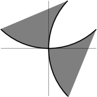
Figure 2.1. $\mbox{\rm lev}_{\leq 0}f$ for $f(x)=(x_{2}-x_{1}^{2})(x_{1}-x_{2}^{2})$ in Example 2.6.

3. Framework for a mountain pass algorithm

In this section, we first present subroutines for a mountain pass algorithm, and then show how the corresponding mountain pass algorithm has local and global properties.

We first present the subroutines that make up the global algorithm.

Algorithm 3.1.

(Subroutines in global mountain pass algorithm) Here are the subroutines that will be the building blocks of our global mountain pass algorithm.

1. (Parallel distance reduction) Given points $z$ and $z^{\prime}$ and a level $l$ such that $f(z)=f(z^{\prime})=l$,

   1. Let $v=z-z^{\prime}$, and let $x$ be any point on the segment $[z,z^{\prime}]$.

   2. From $\nabla f(z)$ and $\nabla f(z^{\prime})$, determine $\nabla(g_{l,v}^{2})(x)$. The Hessian $\nabla^{2}g_{l,v}^{2}(x)$ may also be calculated or estimated for a (quasi-) Newton method. These values will give a direction $d$ for decrease of $g_{l,v}^{2}(\cdot)$.

   3. There is some $t>0$ such that $g_{l,v}(x+td)<g_{l,v}(x)$. Two cases are possible. If $g_{l,v}(x+td)>0$, then $z(x+td)$ and $z^{\prime}(x+td)$ are new iterates reducing the parallel distance. If $g_{l,v}(x+td)=0$, then let $x^{\prime}$ be a local maximum of $f$ on the line $\{x+td\}+\mathbb{R}\{v\}$. We have $f(x^{\prime})\leq l$, and we should run $(l\downarrow)$ below.

2. (Adjusting vector $v$) Given points $z$ and $z^{\prime}$ and a level $l$ such that $f(z)=f(z^{\prime})=l$,

   1. Perturb $z$ and/or $z^{\prime}$ such that we still have $f(z)=f(z^{\prime})=l$, and that $\|z-z^{\prime}\|$ is reduced. The vector $v=z-z^{\prime}$ is now adjusted.

3. (Decrease level $l$) Given $x$ and $v\neq 0$ such that $x$ is a local maximum of $f$ on $\{x\}+\mathbb{R}\{v\}$,

   1. Find local minimizer of $f$ on $\{x\}+\mathbb{R}\{d\}$, where $d\perp v$ and $-\nabla f(x)^{T}d<0$. The direction $d$ can be chosen to be the projection of $-\nabla f(x)$ onto the subspace perpendicular to $v$.

4. (Increase level $l$) Given points $z$ and $z^{\prime}$ and a level $l$ such that $f(z)=f(z^{\prime})=l$,

   1. Choose some $x\in[z,z^{\prime}]$ such that $f(x)>l$. (One choice is $x=\frac{1}{2}(z+z^{\prime})$.) Perturb $z$ and $z^{\prime}$ so that $f(z)$ and $f(z^{\prime})$ equal this new value of $l$.

Other ways of adjusting the vector $v$ apart from (Av) are possible, though they are not as simple as (Av). For example, the vector $v$ can also be calculated by taking the eigenvector corresponding to the negative eigenvalue of $\nabla^{2}f(z_{i})$, $\nabla^{2}f(z_{i}^{\prime})$, or some combination of the two matrices.

We gave a method of decreasing the level $l$ in ($l\downarrow$). Adjustments to the strategy presented in ($l\downarrow$) can be made as needed. For example, the condition $d\perp v$ can be adjusted.

There are also other reasons to adjust $l$. First, the contrapositive of Lemma 4.6(1) later can be roughly interpreted as follows: If $1/|v^{T}u(\nabla f(z))|$ is too small, then the critical level is below $f(z)=l$. We can thus reduce the level $l$. Secondly, when $g_{l,v}(x)$ is too high, signifying that the points $z(x)$ and $z^{\prime}(x)$ are too far apart, one can increase $l$. Third, the points evaluated may not have function value $l$, making a different value more suitable. Lastly, it is possible to estimate $l$ by setting the minimizer of $g_{l,v}(x)^{2}$ to be zero from the formula in (2.1).

3.1. Fast local convergence

We discuss the fast local convergence properties of the level set algorithm. We recall our mountain pass algorithm in [LP11], where we proved local superlinear convergence of a level set algorithm under restrictive assumptions, and show how the difficult steps there can be seen as limiting cases of subroutines (Av) and ($l\downarrow$).

We recall our mountain pass algorithm in [LP11].

Algorithm 3.2.

[LP11] (A local superlinearly convergent algorithm) Let counter $i$ be $0$. Given points $z_{0}$ and $z_{0}^{\prime}$, and a level $l_{0}$ such that $f(z_{0})=f(z_{0}^{\prime})=l_{0}$. Let $U$ be an open neighborhood of the saddle point $\bar{x}$ that contains $z_{0}$ and $z_{0}^{\prime}$.

1. Perturb $z_{i}$ and $z_{i}^{\prime}$ to the points $\tilde{z}_{i}$ and $\tilde{z}_{i}^{\prime}$ so that for some open set $U$, $\tilde{z}_{i}$ and $\tilde{z}_{i}^{\prime}$ are the minimizers of the problem

   $$\min_{x,y} \|x-y\|$$

   s.t. $$x,y\mbox{ lie in the same component }U\cap\mbox{\rm lev}_{\leq l_{i}}f\mbox{ as }z_{i}\mbox{ and }z_{i}^{\prime}\mbox{ respectively.}$$ (3.1)

2. Let $v_{i}$ be the unit vector in the same direction as $\tilde{z}_{i}-\tilde{z}_{i}^{\prime}$. Find the minimum of $f$ on $U\cap L_{i}$, where $L_{i}$ is the perpendicular bisector of $\tilde{z}_{i}$ and $\tilde{z}_{i}^{\prime}$. Let this value be $l_{i+1}$. Find $z_{i+1}$ and $z_{i+1}^{\prime}$ such that they are points in the same components of the level set $U\cap\mbox{\rm lev}_{\leq l_{i+1}}f$ as $\tilde{z}_{i}$ and $\tilde{z}_{i}^{\prime}$ respectively, and that $z_{i+1}-z_{i+1}^{\prime}$ points in the same direction as $v_{i}$.

3. Stop if $\|z_{i+1}-z_{i+1}^{\prime}\|$ is sufficiently small, or until we find a point $x$ such that $\|\nabla f(x)\|$ is sufficiently small. Increase the counter $i$, and return to step 1.

Algorithm 3.2 can be built from the subroutines highlighted in Algorithm 3.1. Step (1) can be seen as applying the step (Av) infinitely many times, while step (2) can be seen as applying one step of ($l\uparrow$), then applying ($l\downarrow$) infinitely often till the minimizer of $f$ on $U\cap L_{i}$ is reached.

The main result in [LP11] is that in some neighborhood $U$ of a nondegenerate saddle point $\bar{x}$ of Morse index one, the steps in Algorithm 3.2 are well defined, and Algorithm 3.2 converges locally superlinearly to $\bar{x}$. This shows that level set methods can satisfy Principle (P1).

However, Algorithm 3.2 has some disadvantages:

• Step 1 in Algorithm 3.2 is difficult to perform in practice. If an alternating projection method was used to solve (3.1) for example, the convergence will be very slow when close to the minimizers.

  

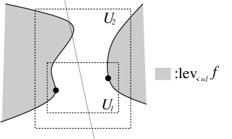
  Figure 3.1. We elaborate on the possible difficulties in finding a lower bound of critical level explained in step 2 of Algorithm 3.2. Let $L$ be the perpendicular bisector of the two closest points as shown. The neighborhood $U_{1}$ is too small as a minimizer of $f$ on $U_{1}\cap L$ does not exist in the relative interior of $U_{1}\cap L$. The neighborhood $U_{2}$ is too large since the minimum value of $f$ on $U_{2}\cap L$ is worse than the previous lower bound on the critical value.

• Related to (D1) is the problem of ensuring that $U\cap\mbox{\rm lev}_{\leq l}f$ is a union of two components for some convex neighborhood $U$ of $\bar{x}$. This in turn requires $l$ to satisfy $l<f(\bar{x})$, where $f(\bar{x})$ is the critical level. Step 2 in Algorithm 3.2 ensures that the calculated level is an underestimate of the critical level, but this step may involve more computational effort than is necessary.

Algorithm 3.2 can be extended to a global algorithm. A few problems may arise in the global case. Firstly, the problem of minimizing $f$ on $L_{i}$ is not necessarily easy. Sometimes, $f$ may not have a local minimizer in $U\cap L_{i}$. Secondly, the new estimate $l$ of the critical level $f(\bar{x})$ may be even lower than the previous estimate, rendering it useless as a lower bound on $f(\bar{x})$. Lastly, the estimate $l$ of the critical level may actually be an upper estimate of $f(\bar{x})$ instead. See Figure 3.1.

Proposition 2.1 suggests that using $g_{l,v}^{2}(\cdot)$ overcomes the difficulties (D1) and (D2). Provided $v$ is close enough to the eigenvector corresponding to the negative eigenvalue of $\nabla f(\bar{x})$, the function $g_{l,v}^{2}(\cdot)$ restricted to any $(n-1)$ dimensional affine space not containing $v$ is the maximum of a quadratic with positive definite Hessian and $0$. One can first minimize $g_{l,v}^{2}(\cdot)$ as a quadratic. Once close enough to $\bar{x}$, the minimizer of the corresponding quadratic, say $\tilde{x}$, will give a good estimate of $\bar{x}$.

3.2. Global convergence results

We now look at the global mountain pass algorithm involving the subalgorithms listed in Algorithm 3.1.

Algorithm 3.3.

(Global mountain pass algorithm) Let the counter $i$ be $0$. Suppose the points $z_{0}$ and $z_{0}^{\prime}$ and a level $l_{0}$ are such that $f(z_{0})=f(z_{0}^{\prime})=l_{0}$. Let $x_{0}$ be some point in the line segment $[z_{0},z_{0}^{\prime}]$. Let $v_{0}=z_{0}-z_{0}^{\prime}$.

1. Run (PD) on $z_{i}$, $z_{i}^{\prime}$, $v_{i}$ and $l_{i}$. Three outcomes are possible:

   1. If the new parallel distance is positive and sufficient decrease in the parallel distance is obtained, let the output be $z_{i+1}$ and $z_{i+1}^{\prime}$. Let $l_{i+1}=l_{i}$. Run (Av), which perturbs either $z_{i+1}$ or $z_{i+1}^{\prime}$. The vector $v_{i+1}$ is set to be the unit vector in the direction of $z_{i+1}-z_{i+1}^{\prime}$.

   2. If the new parallel distance is positive but the parallel distance changed little from previous iterations, run ($l\uparrow$) to perturb $z_{i+1}$ and $z_{i+1}^{\prime}$, and let $l_{i+1}$ be the new level. The vector $v_{i+1}$ equals $v_{i}$, unchanged from before.

   3. If the new parallel distance is zero, then let $l_{i+1}$ be the new level, and let $x_{i+1}$ be the local maximum as stated in (PD). Run ($l\downarrow$). The new level is still labeled as $l_{i+1}$. The vector $v_{i+1}$ equals $v_{i}$, unchanged from before.

2. Increase $i$ by one. If in the course of the calculations, a point $x$ such that $\|\nabla f(x)\|$ is small is encountered, then the algorithm ends. If $\|z_{i}-z_{i}^{\prime}\|$ is small and the distance of $0$ to the convex hull of $\{\nabla f(z_{i}),\nabla f(z_{i}^{\prime})\}$ is small, then we can extrapolate some point $x\in[z_{i},z_{i}^{\prime}]$ for which $\|\nabla f(x)\|$ is small, and end the algorithm. Otherwise, go back to step 1.

In Algorithm 3.3, the subroutines (PD) and (Av) reduce the distance between the components of the level set $U\cap\mbox{\rm lev}_{\leq l}f$. Algorithm 3.3 illustrates just one way to decide which of the subroutines (PD), (Av), ($l\uparrow$) and ($l\downarrow$) to use at each step, and other combinations are possible. There is still flexibility on whether option 1(a) or 1(b) is taken. Once close enough to the saddle point, a quadratic model method can be used.

The basis of (P2) for both Algorithms 3.2 and 3.3 is the following result.

Theorem 3.4.

[LP11](Global convergence of level set algorithm) Let $f:X\to\mathbb{R}$. Suppose $\{a_{i}\}_{i=0}^{\infty}$ and $\{b_{i}\}_{i=0}^{\infty}$ are sequences of points and $\{l_{i}\}_{i=0}^{\infty}$ is a sequence satisfying $l_{i}\nearrow f(\bar{x})$. If $x_{i}$ and $y_{i}$ lie in separate components of $\{x\mid f(x)\leq l_{i}\}$, and $\bar{x}=\lim_{i\to\infty}a_{i}=\lim_{i\to\infty}b_{i}$, then $\bar{x}$ is a saddle point.

One difficulty is to decide whether $a_{i}$ and $b_{i}$ are in different components of $\mbox{\rm lev}_{\leq l_{i}}f$, but we can use $\nabla f(a_{i})$ and $\nabla f(b_{i})$ to make a guess. Note that provided the limits exist, $\lim_{i\to\infty}a_{i}=\lim_{i\to\infty}b_{i}$ is equivalent to $\lim_{i\to\infty}\|a_{i}-b_{i}\|=0$. This principle can be seen as a convergence property of Algorithms 3.2 and 3.3. It is therefore pragmatic to decrease the distance or parallel distance between the components of the level sets, especially at the start of a global mountain pass algorithm where the quadratic approximation is not valid yet. The problem of choosing the sequence $\{l_{i}\}_{i=0}^{\infty}$ is much more difficult. The strategy in Algorithm 3.3 is adequate for our numerical experiment, but more still needs to be done.

4. Independence of $l$ in estimating $\nabla^{2}(g_{l,v}^{2})(\cdot)$

We recall that in our level set algorithm in Section 3, we perturb the level $l$ using subroutines $(l\uparrow)$ and $(l\downarrow)$ so that $l$ converges to the critical value $f(\bar{x})$ of the saddle point $\bar{x}$. Such changes in $l$ can be quite sudden. The Hessian $\nabla^{2}(g_{l,v}^{2})(\cdot)$ is not continuous at $\bar{x}$ because of the $\frac{1}{v^{T}f(z)}$ in its formula, and the continuity at an $x$ where $\nabla^{2}(g_{l,v}^{2})(\cdot)$ is only good enough for small changes in $l$. In this section, we show in Theorem 4.9 that there is a neighborhood $U$ of the saddle point $\bar{x}$ such that as long as $l<f(\bar{x})$ is close enough to $f(\bar{x})$ and $v$ is close enough to the eigenspace corresponding to the negative eigenvalue of $\nabla^{2}(g_{l,v}^{2})(\bar{x})$, the Hessian $\nabla^{2}(g_{l,v}^{2})(x)$ for $x\in U$ can be estimated from a quadratic model of $f$ at $\bar{x}$. Such a result shows that under changes of $l$ near $\bar{x}$, the Hessian $\nabla^{2}(g_{l,v}^{2})(\cdot)$ does not depend too much on $l$, making previous estimates of $\nabla^{2}(g_{l,v}^{2})(\cdot)$ useful for future iterations. As a consequence, we obtain the convexity of $g_{l,v}(\cdot)^{2}$.

First, we have the following result that allows us to identify convexity.

Proposition 4.1.

(Convexity from positive definite Hessians) Suppose $f:\mathbb{R}^{n}\to[0,\infty)$ is a continuous function that is $\mathcal{C}^{2}$ at all points $x$ satisfying $f(x)>0$, and the corresponding Hessian $\nabla^{2}f(x)$ is positively semidefinite. Then $f$ is convex. (The issue here is that the nonsmoothness of $f$ on the boundary of $\{x\mid f(x)=0\}$ does not affect convexity.)

Proof.

The usual convexity test $tf(x)+(1-t)f(y)\geq f(tx+(1-t)y)$ for all $x,y\in\mathbb{R}^{n}$ and $t\in(0,1)$ allows us to reduce the problem in $\mathbb{R}^{n}$ to that of $n=1$. We first notice that there cannot exist $x_{1},x_{2}\in\mathbb{R}$ such that $x_{1}<\tilde{x}<x_{2}$, $f(x_{1})=f(x_{2})=0$, and $f(x)>0$ for all $x\in(x_{1},x_{2})$, since this is a contradiction to the convexity of $f$ on $(x_{1},x_{2})$.

Using the above property, we can find $x_{3},x_{4}\in\mathbb{R}\cup\{-\infty,\infty\}$ such that $x_{3}\leq x_{4}$ and

$$f(x)\ \begin{cases}=0&\mbox{ if }x\in[x_{3},x_{4}]\\ >0&\mbox{ if }x\notin[x_{3},x_{4}].\end{cases}$$

Note that one or both of $x_{3}$ and $x_{4}$ might be $\pm\infty$. It is an easy exercise that the subdifferential mapping $\partial f$ is monotone, thus $f$ is convex. ∎

We shall make use of Proposition 4.1 to establish the convexity of $g_{l,v}^{2}$ by making sure that the Hessian $\nabla^{2}(g_{l,v}^{2})$ is positive semidefinite whenever $g_{l,v}>0$.

We make some simplifying assumptions for the rest of this section.

Assumption 4.2.

(Smooth $f$) Assume that $f:\mathbb{R}^{n}\to\mathbb{R}$ is a $\mathcal{C}^{2}$ function with a nondegenerate critical point $\bar{x}=0$ of Morse index one satisfying $f(0)=0$ such that $H=\nabla^{2}f(0)$ is diagonal with entries arranged in decreasing manner as $\lambda_{1},\dots,\lambda_{n}$. This means that the diagonal entries of $\nabla^{2}f(0)$ consist of $n-1$ positive eigenvalues and one negative eigenvalue. Let the eigenvector corresponding to the negative eigenvalue $\lambda_{n}$ be $\bar{v}$.

We also make another definition that will simplify many of the statements in this section. Denote $\bar{f}_{\delta}:\mathbb{R}^{n}\to\mathbb{R}$ by

$$\bar{f}_{\delta}(x)=\frac{1}{2}x^{T}[\nabla^{2}f(0)+\delta I]x.$$ (4.1)

Let $\bar{g}_{\delta,l,v}$ be the value of $g_{l,v}$ defined through the quadratic $\bar{f}_{\delta}(\cdot)$ (instead of through $f(\cdot)$). The values $\bar{z}_{\delta}(x)$ and $\bar{z}_{\delta}^{\prime}(x)$, defined through $\bar{f}_{\delta}$ will be of use later in this section. We write $\bar{f}=\bar{f}_{0}$, $\bar{g}_{l,v}=\bar{g}_{0,l,v}$, $\bar{z}(\cdot)=\bar{z}_{0}(\cdot)$ and $\bar{z}^{\prime}(\cdot)=\bar{z}_{0}^{\prime}(\cdot)$. We also write $H_{\delta}=\nabla^{2}f(0)+\delta I$ to simplify notation.

Definition 4.3.

(Continuity condition) For a function $f:\mathbb{R}^{n}\to\mathbb{R}$ satisfying Assumption 4.2, $\delta>0$, $\gamma>0$ and convex neighborhoods $U_{\delta}$ and $U_{\delta}^{\prime}$ of $0$ such that $U_{\delta}\subset U_{\delta}^{\prime}$, we say that condition $P(f,\delta,\gamma,U_{\delta},U_{\delta}^{\prime})$ is satisfied if

1. $\|\nabla^{2}f(x)-\nabla^{2}f(0)\|\leq\delta$ for all $x\in U_{\delta}^{\prime}$,

2. For $\bar{f}_{\delta}:\mathbb{R}^{n}\to\mathbb{R}$ and $\bar{S}_{\delta,l,v}(\cdot)$ as defined in (2.2), we have $\bar{S}_{\delta,l,v}(x)\subset U_{\delta}^{\prime}$ for all $x\in U_{\delta}$ and $l\in(-\gamma,0]$.

It is clear through Proposition 2.2 and the continuity of the Hessian that for any $\delta>0$, there must be convex neighborhoods $U_{\delta}$ and $U_{\delta}^{\prime}$ such that $U_{\delta}\subset U_{\delta}^{\prime}$ and $P(f,\delta,\gamma,U_{\delta},U_{\delta}^{\prime})$ holds. It is also clear that if $P(f,\delta,\gamma,U_{\delta},U_{\delta}^{\prime})$ holds, we have

$$\frac{1}{2}x^{T}[\nabla^{2}f(0)-\delta I]x\leq f(x)\leq\frac{1}{2}x^{T}[\nabla^{2}f(0)+\delta I]x\mbox{ for all }x\in U_{\delta}.$$ (4.2)

The next result is a bound on the error in $z(x)$.

Lemma 4.4.

(Controlling $\bar{z}(x)$) Suppose that $f:\mathbb{R}^{n}\to\mathbb{R}$ is $\mathcal{C}^{2}$ and satisfies Assumption 4.2. Let $v$ be a unit vector such that $v^{T}\nabla^{2}f(0)v<0$. For any $\epsilon>0$, there are $\delta>0$, $\gamma>0$ and convex neighborhoods $U_{\delta}$ and $U_{\delta}^{\prime}$ of $0$ such that $P(f,\delta,\gamma,U_{\delta},U_{\delta}^{\prime})$ holds, and for all $x\in U_{\delta}$ and $l\in(-\gamma,0]$, we have

$$\|\bar{z}(x)-z(x)\| \leq \epsilon\|\bar{z}(x)\|,$$

$$\|\bar{z}^{\prime}(x)-z^{\prime}(x)\| \leq \epsilon\|\bar{z}(x)\|,$$

$$\mbox{and }|\bar{g}_{l,v}(x)-g_{l,v}(x)| \leq \epsilon\|\bar{z}(x)\|.$$

Proof.

Since $z(x)$ and $\bar{z}(x)$ lie inside the line segment $[\bar{z}_{\delta}(x),\bar{z}_{-\delta}(x)]$, we have $\|\bar{z}(x)-z(x)\|\leq\|\bar{z}_{\delta}(x)-\bar{z}_{-\delta}(x)\|$. Since $\bar{z}_{\delta}(x)$, $\bar{z}_{-\delta}(x)$, $\bar{z}_{-\delta}^{\prime}(x)$ and $\bar{z}_{\delta}^{\prime}(x)$ line up in a line (with direction $v$) in that order, we have

$$\|\bar{z}_{\delta}(x)-\bar{z}_{-\delta}(x)\| < \|\bar{z}_{\delta}(x)-\bar{z}_{-\delta}(x)\|+\|\bar{z}_{\delta}^{\prime}(x)-\bar{z}_{-\delta}^{\prime}(x)\|$$

$$= \bar{g}_{\delta,l,v}(x)-\bar{g}_{-\delta,l,v}(x).$$

Similarly,

$$|\bar{g}_{l,v}(x)-g_{l,v}(x)| < \|\bar{z}_{\delta}(x)-\bar{z}_{-\delta}(x)\|+\|\bar{z}_{\delta}^{\prime}(x)-\bar{z}_{-\delta}^{\prime}(x)\|$$

$$= \bar{g}_{\delta,l,v}(x)-\bar{g}_{-\delta,l,v}(x).$$

Our goal is therefore to prove that for every $\epsilon>0$, we can find a $\delta>0$ such that $\bar{g}_{\delta,l,v}(x)-\bar{g}_{-\delta,l,v}(x)\leq\epsilon\|\bar{z}(x)\|$ for all $x\in\mathbb{R}^{n}$.

Note that our problem has now been transformed to a new problem on an exact quadratic $\bar{f}(\cdot)$.

The treatment for the case $l=0$ and $l<0$ are different, and we start off by treating the case $l=0$.

CASE $l=0$: For a point $x\in\mathbb{R}^{n}$, the sets $\mbox{\rm lev}_{\leq 0}\bar{f}_{\delta}$ and $\mbox{\rm lev}_{\leq 0}\bar{f}_{-\delta}$ are cones, with $\mbox{\rm lev}_{\leq 0}\bar{f}_{\delta}\subset\mbox{\rm lev}_{\leq 0}\bar{f}_{-\delta}$. For $\delta>0$ small enough, $\nabla^{2}f(0)$ consists of $n-1$ positive eigenvalues and one negative eigenvalue, so $\mbox{\rm lev}_{\leq 0}\bar{f}_{\delta}$ and $\mbox{\rm lev}_{\leq 0}\bar{f}_{-\delta}$ are both the union of two convex cones intersecting only at $0$. For a point $x$, the points $\bar{z}_{\delta}(x)$, $\bar{z}_{-\delta}(x)$, $\bar{z}_{\delta}^{\prime}(x)$ and $\bar{z}_{-\delta}^{\prime}(x)$ can be calculated easily from the quadratic formulas we have seen in the proof of previous results (in particular, Proposition 2.1), giving

$$\bar{g}_{\delta,l,v}(x) = \|\bar{z}_{\delta}(x)-\bar{z}_{\delta}^{\prime}(x)\|=\frac{2\sqrt{[v^{T}H_{\delta}x]^{2}-[v^{T}H_{\delta}v][x^{T}H_{\delta}x]}}{v^{T}H_{\delta}v}$$

$$\mbox{and }\bar{g}_{-\delta,l,v}(x) = \|\bar{z}_{-\delta}(x)-\bar{z}_{-\delta}^{\prime}(x)\|=\frac{2\sqrt{[v^{T}H_{-\delta}x]^{2}-[v^{T}H_{-\delta}v][x^{T}H_{-\delta}x]}}{v^{T}H_{-\delta}v}.$$

Consider the problem

$$\max_{x\in\partial\mathbb{B}}h_{\delta}(x),$$

where $h_{\delta}(x)=\bar{g}_{\delta,l,v}(x)-\bar{g}_{-\delta,l,v}(x)$. The function $h_{\delta}(\cdot)$ is continuous, and the set $\partial\mathbb{B}:=\{x:\|x\|=1\}$ is compact. The optimization problem above satisfies the conditions in Proposition 4.5, so for any $\epsilon>0$, we can choose $\delta>0$ such that $\max_{x\in\partial\mathbb{B}}h_{\delta}(x)<\epsilon$. We have

$$h_{\delta}(\bar{z}(x))\leq\|\bar{z}(x)\|\max_{y\in\partial\mathbb{B}}h_{\delta}(y)<\epsilon\|\bar{z}(x)\|.$$

CASE $l<0$: We can consider the case $l=-1/2$ first. The other cases follow by a scaling.

If $\|x\|>1/\sqrt{\delta}$, then $\bar{f}_{2\delta}(x)\leq 0$ implies that $\bar{f}_{\delta}(x)=\bar{f}_{2\delta}(x)-\frac{1}{2}\delta\|x\|^{2}\leq-\frac{1}{2}$. Also, $\bar{f}_{-\delta}(x)\leq-\frac{1}{2}$ clearly implies $\bar{f}_{-2\delta}(x)\leq\bar{f}_{-\delta}(x)\leq 0$. This gives

$$\left[\frac{1}{\sqrt{\delta}}\mathbb{B}\right]^{C}\cap\mbox{\rm lev}_{\leq 0}\bar{f}_{2\delta} \subset \left[\frac{1}{\sqrt{\delta}}\mathbb{B}\right]^{C}\cap\mbox{\rm lev}_{\leq-1/2}\bar{f}_{\delta}$$

$$\subset \left[\frac{1}{\sqrt{\delta}}\mathbb{B}\right]^{C}\cap\mbox{\rm lev}_{\leq-1/2}\bar{f}_{-\delta}$$

$$\subset \left[\frac{1}{\sqrt{\delta}}\mathbb{B}\right]^{C}\cap\mbox{\rm lev}_{\leq 0}\bar{f}_{-2\delta},$$

where $[\cdot]^{C}$ is the complementation of a set. By the treatment for the case $l=0$, for any $\epsilon>0$, we can find $\delta_{1}>0$ such that if $\|\bar{z}(x)\|>1/\sqrt{\delta_{1}}$, then $\|\bar{z}_{\delta_{1}}(x)-\bar{z}_{-\delta_{1}}(x)\|<\frac{\epsilon}{2}\|\bar{z}(x)\|$. Therefore, if $\delta_{2}\in(0,\delta_{1})$, we have $\|\bar{z}_{\delta_{2}}(x)-\bar{z}_{-\delta_{2}}(x)\|<\frac{\epsilon}{2}\|\bar{z}(x)\|$, which gives

$$\bar{g}_{\delta,l,v}(x)-\bar{g}_{-\delta,l,v}(x)\leq\epsilon\|\bar{z}(x)\|.$$

We still need to treat the case where $\|\bar{z}(x)\|\leq 1/\sqrt{\delta_{1}}$. The condition $\bar{f}(\bar{z}(x))=-\frac{1}{2}$ implies that $\|\bar{z}(x)\|\geq 1/\sqrt{-\lambda_{n}+2\delta_{1}}$, where $\lambda_{n}$ is the negative eigenvalue of $\nabla^{2}f(0)$. We make use of the same strategy to estimate $\|\bar{z}_{\delta}(x)-\bar{z}_{-\delta}(x)\|$ as in the last case. This time, the formulas give

$$\bar{g}_{\delta,l,v}(x)-\bar{g}_{-\delta,l,v}(x) = \frac{2\sqrt{[v^{T}H_{\delta}x]^{2}-[v^{T}H_{\delta}v][x^{T}H_{\delta}x-2l]}}{v^{T}H_{\delta}v}$$

$$-\frac{2\sqrt{[v^{T}H_{-\delta}x]^{2}-[v^{T}H_{-\delta}v][x^{T}H_{-\delta}x-2l]}}{v^{T}H_{-\delta}v}.$$

We are led to consider the problem

$$\max_{x\in C}h_{\delta}(x),$$

where

$$h_{\delta}(x) := \bar{g}_{\delta,l,v}(x)-\bar{g}_{-\delta,l,v}(x),$$

$$\mbox{ and }C = \big{\{}y:1/\sqrt{-\lambda_{n}+2\delta_{1}}\leq\|y\|\leq 1/\sqrt{\delta_{1}}\big{\}}.$$

Once again, $h_{\delta}(\cdot)$ is continuous, $C$ is compact, and Proposition 4.5 can be applied. There is some $\delta_{2}$ such that $0<\delta_{2}<\delta_{1}$ and $\max_{x\in C}h_{\delta_{2}}(x)<\epsilon/\sqrt{-\lambda_{n}+2\delta_{1}}$. If $\|\bar{z}(x)\|\in[1/\sqrt{-\lambda_{n}+2\delta_{1}},1/\sqrt{\delta_{1}}]$, then we have

$$h_{\delta_{2}}\big{(}\bar{z}(x)\big{)}\leq\epsilon/\sqrt{-\lambda_{n}+2\delta_{1}}\leq\epsilon\|\bar{z}(x)\|.$$

The case where $l$ is another negative number differ from the case $l=-1/2$ by a scaling. Our claim follows. ∎

Here is a result that we have used for Lemma 4.4.

Proposition 4.5.

(Convergence to zero of maximum value) Suppose that $h_{\delta}:C\to\mathbb{R}$ is continuous for all $\delta\geq 0$, $C$ is compact, and that $\delta_{1}<\delta_{2}$ implies $h_{\delta_{1}}(x)\leq h_{\delta_{2}}(x)$ for all $x\in C$. Assume also that for all $x\in C$, $h_{\delta}(x)\searrow 0$ as $\delta\searrow 0$. Then $\max_{x\in C}h_{\delta}(x)\searrow 0$ as $\delta\searrow 0$.

Proof.

For each sequence $\delta_{i}\searrow 0$ as $i\nearrow\infty$, there is a maximizer $\tilde{x}_{i}$ such that $h_{\delta_{i}}(\tilde{x}_{i})=\max_{x\in C}h_{\delta_{i}}(x)$. It suffices to show that $h_{\delta_{i}}(\tilde{x}_{i})\searrow 0$ as $i\nearrow\infty$. Due to the compactness of $C$, we can assume that there is a subsequence of $\{\tilde{x}_{i}\}$ converging to some $\tilde{x}\in C$. For any $\epsilon>0$, there is some $a$ such that $h_{\delta_{a}}(\tilde{x})<\epsilon$ and a neighborhood $U_{\epsilon}$ of $\tilde{x}$ such that $h_{\delta_{a}}(x)<2\epsilon$ for all $x\in U_{\epsilon}$. This means that some tail of the sequence $\{h_{\delta_{i}}(\tilde{x}_{i})\}_{i=1}^{\infty}$ is less than $2\epsilon$. Since $\epsilon$ is arbitrary, $\max_{x\in C}h_{\delta_{i}}(x)=h_{\delta_{i}}(\tilde{x}_{i})\searrow 0$ as $i\nearrow\infty$ as needed. ∎

For $x\neq 0$, let $u(x)=x/\|x\|$. Here are some bounds we need to check:

Lemma 4.6.

(Uniform bounds on terms) Suppose that $\bar{f}:\mathbb{R}^{n}\to\mathbb{R}$ is defined by $\bar{f}(x)=\frac{1}{2}x^{T}\nabla^{2}f(0)x$, where $f:\mathbb{R}^{n}\to\mathbb{R}$ is a function satisfying Assumption 4.2. Let $\bar{v}$ be the eigenvector corresponding to the negative eigenvalue of $\nabla^{2}f(0)$. Assume that $v$ is a unit vector such that $\|v-\bar{v}\|<\alpha$. Let $\bar{z}$ be a point such that $f(\bar{z})\leq 0$. We have the following:

1. $1/|v^{T}u(\nabla\bar{f}(\bar{z}))|<1/\left[\sqrt{\frac{-\lambda_{n}}{\max(\lambda_{1},-\lambda_{n})-\lambda_{n}}}-\alpha\right]$ for all $\bar{z}$ such that $\bar{f}(\bar{z})\leq 0$.

2. $\frac{\bar{g}_{l,v}(\bar{z})}{\|\nabla\bar{f}(\bar{z})\|}\leq\frac{2}{|\lambda_{n}|-2\alpha|\lambda_{n}|-\alpha^{2}\max(\lambda_{1},-\lambda_{n})}$ for all $\bar{z}$ satisfying $f(\bar{z})=l$, where $l\leq 0$.

Proof.

Let $H$ be $\nabla^{2}f(0)$, which we recall is diagonal. We prove (1) and (2).

(1) We have

$$|v^{T}u(\nabla\bar{f}(\bar{z}(x)))| \geq |\bar{v}^{T}u(\nabla\bar{f}(\bar{z}))|-|(v-\bar{v})^{T}u(\nabla\bar{f}(\bar{z}))|$$

$$\geq \left|\bar{v}^{T}\frac{H\bar{z}}{\|H\bar{z}\|}\right|-\alpha$$

$$= \left|\frac{\lambda_{n}\bar{z}_{n}}{\sqrt{\sum_{i=1}^{n}\lambda_{i}^{2}\bar{z}_{i}^{2}}}\right|-\alpha.$$

From the fact that $f(\bar{z})\leq 0$, we have

$$\sum_{i=1}^{n}\lambda_{i}\bar{z}_{i}^{2} \leq 0$$

$$\Rightarrow\lambda_{n}^{2}\bar{z}_{n}^{2} \geq -\lambda_{n}\sum_{i=1}^{n-1}\lambda_{i}\bar{z}_{i}^{2}.$$

Therefore

$$\left(\frac{\lambda_{n}\bar{z}_{n}}{\sqrt{\sum_{i=1}^{n}\lambda_{i}^{2}\bar{z}_{i}^{2}}}\right)^{2} = \frac{\lambda_{n}^{2}\bar{z}_{n}^{2}}{\sum_{i=1}^{n}\lambda_{i}^{2}\bar{z}_{n}^{2}}$$

$$\geq \frac{-\lambda_{n}\sum_{i=1}^{n-1}\lambda_{i}\bar{z}_{i}^{2}}{\sum_{i=1}^{n-1}\lambda_{i}^{2}\bar{z}_{n}^{2}-\lambda_{n}\sum_{i=1}^{n-1}\lambda_{i}\bar{z}_{i}^{2}}$$

$$\geq \frac{-\lambda_{n}\sum_{i=1}^{n-1}\lambda_{i}\bar{z}_{i}^{2}}{\max(\lambda_{1},-\lambda_{n})\sum_{i=1}^{n-1}\lambda_{i}\bar{z}_{n}^{2}-\lambda_{n}\sum_{i=1}^{n-1}\lambda_{i}\bar{z}_{i}^{2}}$$

$$= \frac{-\lambda_{n}}{\max(\lambda_{1},-\lambda_{n})-\lambda_{n}}.$$

The rest of the claim is straightforward.

(2) Through calculations we have seen in the proof of Lemma 4.4, we have

$$\bar{g}_{l,v}(\bar{z})=2\left|\frac{\sqrt{[v^{T}H\bar{z}]^{2}-[v^{T}Hv][\bar{z}^{T}H\bar{z}-2l]}}{v^{T}Hv}\right|=2\left|\frac{v^{T}H\bar{z}}{v^{T}Hv}\right|,$$

since $l=f(\bar{z})=\frac{1}{2}\bar{z}^{T}H\bar{z}$. Now,

$$|v^{T}Hv| \geq |\bar{v}^{T}H\bar{v}|-2|(v-\bar{v})^{T}H\bar{v}|-|(v-\bar{v})^{T}H(v-\bar{v})|$$

$$\geq |\lambda_{n}|-2\alpha|\lambda_{n}|-\alpha^{2}\max(\lambda_{1},-\lambda_{n}).$$

Finally,

$$\frac{\bar{g}_{l,v}(\bar{z})}{\|\nabla\bar{f}(\bar{z})\|} = \frac{2|v^{T}H\bar{z}|}{\|H\bar{z}\||v^{T}Hv|}$$

$$\leq \frac{2\|v\|\|H\bar{z}\|}{\|H\bar{z}\|[|\lambda_{n}|-2\alpha|\lambda_{n}|-\alpha^{2}\max(\lambda_{1},-\lambda_{n})]}$$

$$= \frac{2}{|\lambda_{n}|-2\alpha|\lambda_{n}|-\alpha^{2}\max(\lambda_{1},-\lambda_{n})}.$$

∎

We will use the following result.

Proposition 4.7.

(Products and norms) Let $A_{i}$ and $\bar{A}_{i}$, where $i=1,\dots,k$, be matrices such that the products $A_{1}A_{2}\cdots A_{k}$ and $\bar{A}_{1}\bar{A}_{2}\cdots\bar{A}_{k}$ are valid. Then

$$\|A_{1}A_{2}\cdots A_{k}-\bar{A}_{1}\bar{A}_{2}\cdots\bar{A}_{k}\|\leq\left[\prod_{i=1}^{k}(\|\bar{A}_{i}\|+\|A_{i}-\bar{A}_{i}\|)\right]-\prod_{i=1}^{k}\|\bar{A}_{i}\|.$$ (4.3)

Proof.

The formula follows readily from

$$A_{1}A_{2}\cdots A_{k}-\bar{A}_{1}\bar{A}_{2}\cdots\bar{A}_{k}=[\bar{A}_{1}+(A_{1}-\bar{A}_{1})]\cdots[\bar{A}_{k}+(A_{k}-\bar{A}_{k})]-\bar{A}_{1}\bar{A}_{2}\cdots\bar{A}_{k}.$$

∎

Lemma 4.8.

(Uniform bounds on differences) Suppose $f:\mathbb{R}^{n}\to\mathbb{R}$ satisfies Assumption 4.2. Assume that $v$ is a unit vector such that $\|v-\bar{v}\|<\alpha$. For every $\epsilon>0$, there exists $\delta>0$, $\gamma>0$ and convex neighborhoods $U_{\delta}$ and $U_{\delta}^{\prime}$ of $0$ such that $P(f,\delta,\gamma,U_{\delta},U_{\delta}^{\prime})$ holds, and for all $x\in U_{\delta}$, we have

1. $\|u(\nabla\bar{f}(\bar{z}(x)))-u(\nabla f(z(x)))\|<\epsilon$.

2. $\left|\frac{1}{u(\nabla\bar{f}(\bar{z}(x)))^{T}v}-\frac{1}{u(\nabla f(z(x)))^{T}v}\right|<\epsilon$.

3. $\left|\frac{\bar{g}_{l,v}(\bar{z})}{\|\nabla\bar{f}(\bar{z}(x))\|}-\frac{g_{l,v}(z)}{\|\nabla f(z(x))\|}\right|<\epsilon$, where $f\big{(}\bar{z}(x)\big{)}=l$ and $l\in(-\gamma,0]$.

Proof.

We use Lemma 4.4, which says that for $\epsilon_{1}>0$, there are $\delta>0$, $\gamma>0$ and convex neighborhoods $U_{\delta}$ and $U_{\delta}^{\prime}$ of $0$ such that $P(f,\delta,\gamma,U_{\delta},U_{\delta}^{\prime})$ holds, and $\|\bar{z}(x)-z(x)\|\leq\epsilon_{1}\|\bar{z}(x)\|$ for all $x\in U_{\delta}$.

(1) We can easily obtain $\|z(x)\|\leq(1+\epsilon_{1})\|\bar{z}(x)\|$. Let $H=\nabla^{2}f(0)$. Now,

$$\|\nabla\bar{f}(\bar{z}(x))-\nabla f(z(x))\| \leq \|\nabla\bar{f}(\bar{z}(x))-\nabla\bar{f}(z(x))\|+\|\nabla\bar{f}(z(x))-\nabla f(z(x))\|$$

$$\leq \|H(\bar{z}(x)-z(x))\|+\left\|Hz(x)-\int_{0}^{1}\nabla^{2}f(tz(x))dt\cdot z(x)\right\|$$

$$\leq \epsilon_{1}\|H\|\|\bar{z}(x)\|+\|z(x)\|\left\|H-\int_{0}^{1}\nabla^{2}f(tz(x))dt\right\|$$

$$\leq \epsilon_{1}\|\bar{z}(x)\|\|H\|+\delta(1+\epsilon_{1})\|\bar{z}\|$$

$$= \|\bar{z}(x)\|[\epsilon_{1}\|H\|+\delta(1+\epsilon_{1})].$$

Note that the term $[\epsilon_{1}\|H\|+\delta(1+\epsilon_{1})]$ can be made arbitrarily small. Note that $\frac{\|\nabla\bar{f}(\bar{z}(x))\|}{\|\bar{z}(x)\|}\geq\min(|\lambda_{n-1}|,|\lambda_{n}|)$, so

$$\frac{\|\nabla\bar{f}(\bar{z}(x))-\nabla f(z(x))\|}{\|\nabla\bar{f}(\bar{z}(x))\|}\leq\frac{[\epsilon_{1}\|H\|+\delta(1+\epsilon_{1})]}{\min(|\lambda_{n-1}|,|\lambda_{n}|)}.$$ (4.4)

Next, for any $w_{1},w_{2}\in\mathbb{R}^{n}\backslash\{0\}$, we have

$$\left\|\frac{w_{1}}{\|w_{1}\|}-\frac{w_{2}}{\|w_{2}\|}\right\| \leq \left\|\frac{w_{1}}{\|w_{1}\|}-\frac{w_{2}}{\|w_{1}\|}\right\|+\left\|\frac{w_{2}}{\|w_{1}\|}-\frac{w_{2}}{\|w_{2}\|}\right\|$$ (4.5)

$$\leq \frac{\|w_{1}-w_{2}\|}{\|w_{1}\|}+\frac{\|w_{2}\|\left|\|w_{2}\|-\|w_{1}\|\right|}{\|w_{1}\|\|w_{2}\|}$$

$$\leq 2\frac{\|w_{1}-w_{2}\|}{\|w_{1}\|}.$$

Apply the observation in (4.5) to (4.4) to get what we need.

(2) Let $M=\left[\sqrt{\frac{-\lambda_{n}}{\max(\lambda_{1},-\lambda_{n})-\lambda_{n}}}-\alpha\right]^{-1}$. We have from Lemma 4.6(1) that $\frac{1}{|u(\nabla\bar{f}(\bar{z}(x)))^{T}v|}\leq M$. From (1), for $\epsilon_{1}>0$, there exist $\delta>0$, $\gamma>0$ and convex neighborhoods $U_{\delta}$ and $U_{\delta}^{\prime}$ of $0$ such that $P(f,\delta,\gamma,U_{\delta},U_{\delta}^{\prime})$ holds, and $|u(\nabla\bar{f}(\bar{z}(x)))^{T}v-u(\nabla f(z(x)))^{T}v|<\epsilon_{1}$ for all $x\in U_{\delta}$. First,

$$|u(\nabla f(z(x)))^{T}v| \geq |u(\nabla\bar{f}(\bar{z}(x)))^{T}v|-|u(\nabla\bar{f}(\bar{z}(x)))^{T}v-u(\nabla f(z(x)))^{T}v|$$

$$\geq \frac{1}{M}-\epsilon_{1}$$

$$\Rightarrow\frac{1}{|u(\nabla f(z(x)))^{T}v|} \leq \frac{M}{1-\epsilon_{1}M}.$$

Next,

$$\left|\frac{1}{u(\nabla\bar{f}(\bar{z}(x)))^{T}v}-\frac{1}{u(\nabla f(z(x)))^{T}v}\right| = \frac{|v^{T}[u(\nabla\bar{f}(\bar{z}(x)))-u(\nabla f(z(x)))]|}{|u(\nabla\bar{f}(\bar{z}(x)))^{T}v||u(\nabla f(z(x)))^{T}v|}$$

$$\leq M\frac{M}{1-\epsilon_{1}M}\|u(\nabla\bar{f}(\bar{z}(x)))-u(\nabla f(z(x)))\|$$

$$\leq \frac{M^{2}}{1-\epsilon_{1}M}\epsilon_{1}.$$

As the RHS converges to zero as $\epsilon_{1}\searrow 0$, we are done.

(3) We use Proposition 4.7 to get

$$\left|\frac{\bar{g}_{l,v}(\bar{z})}{\|\nabla\bar{f}(\bar{z}(x))\|}-\frac{g_{l,v}(z)}{\|\nabla f(z(x))\|}\right|$$

$$\leq [|\bar{g}_{l,v}(\bar{z})-g_{l,v}(z)|+|\bar{g}_{l,v}(\bar{z})|]\left[\left|\frac{1}{\|\nabla\bar{f}(\bar{z}(x))\|}\right|+\left|\frac{1}{\|\nabla\bar{f}(\bar{z}(x))\|}-\frac{1}{\|\nabla f(z(x))\|}\right|\right]$$

$$-\frac{|\bar{g}_{l,v}(\bar{z})|}{\|\nabla\bar{f}(\bar{z}(x))\|}$$

$$= \left[\frac{|\bar{g}_{l,v}(\bar{z})-g_{l,v}(z)|}{\|\nabla\bar{f}(\bar{z}(x))\|}+\frac{|\bar{g}_{l,v}(\bar{z})|}{\|\nabla\bar{f}(\bar{z}(x))\|}\right]\left[1+\left|1-\frac{\|\nabla\bar{f}(\bar{z}(x))\|}{\|\nabla f(z(x))\|}\right|\right]-\frac{|\bar{g}_{l,v}(\bar{z})|}{\|\nabla\bar{f}(\bar{z}(x))\|}.$$

By Lemma 4.4, for any $\epsilon_{1}>0$, there exist $\delta>0$, $\gamma>0$ and convex neighborhoods $U_{\delta}$ and $U_{\delta}^{\prime}$ of $0$ such that $P(f,\delta,\gamma,U_{\delta},U_{\delta}^{\prime})$ holds, and $|\bar{g}_{l,v}(\bar{z})-g_{l,v}(z)|\leq\epsilon_{1}\|\bar{z}(x)\|$ for all $x\in U_{\delta}$. So

$$\frac{|\bar{g}_{l,v}(\bar{z})-g_{l,v}(z)|}{\|\nabla\bar{f}(\bar{z}(x))\|} \leq \frac{\epsilon_{1}\|\bar{z}(x)\|}{\min(\lambda_{n-1},|\lambda_{n}|)\|\bar{z}(x)\|}$$

$$\leq \frac{\epsilon_{1}}{\min(\lambda_{n-1},|\lambda_{n}|)}.$$

Next, we may reduce $\delta$ if necessary so that $\|\nabla f(z(x))-\nabla\bar{f}(\bar{z}(x))\|\leq\epsilon_{1}\|\bar{z}(x)\|$for all $x\in U_{\delta}$ as well. We have

$$\left|1-\frac{\|\nabla\bar{f}(\bar{z}(x))\|}{\|\nabla f(z(x))\|}\right| = \frac{\left|\|\nabla f(z(x))\|-\|\nabla\bar{f}(\bar{z}(x))\|\right|}{\|\nabla f(z(x))\|}$$

$$\leq \frac{\|\nabla f(z(x))-\nabla\bar{f}(\bar{z}(x))\|}{\|\nabla f(z(x))\|}$$

$$\leq \frac{\|\nabla f(z(x))-\nabla\bar{f}(\bar{z}(x))\|}{\|\nabla\bar{f}(\bar{z}(x))\|-\|\nabla\bar{f}(\bar{z}(x))-\nabla f(z(x))\|}$$

$$\leq \frac{\epsilon_{1}\|\bar{z}(x)\|}{\min(|\lambda_{n}|,|\lambda_{n-1}|)\|\bar{z}(x)\|-\epsilon_{1}\|\bar{z}(x)\|}$$

$$= \frac{\epsilon_{1}}{\min(|\lambda_{n}|,|\lambda_{n-1}|)-\epsilon_{1}}.$$

The RHS of both previous formulas converge to zero as $\epsilon_{1}\searrow 0$, and $\frac{|\bar{g}_{l,v}(\bar{z})|}{\|\nabla\bar{f}(\bar{z}(x))\|}$ is uniformly bounded by Lemma 4.6(2). We have (3) as needed. ∎

We have the following theorem.

Theorem 4.9.

(Hessian behavior and convexity) Let $f:\mathbb{R}^{n}\to\mathbb{R}$ be such that $f$ is $\mathcal{C}^{2}$ in a neighborhood of a nondegenerate critical point $\bar{x}$ with Morse index one, and let $\bar{v}$ be the eigenvector corresponding to the negative eigenvalue of $\nabla^{2}f(\bar{x})$. Let $v$ be a unit vector such that $\|v-\bar{v}\|=\alpha$ is small. Then for any $\epsilon>0$, there are $\delta>0$, $\gamma>0$ and convex neighborhoods $U_{\delta}$ and $U_{\delta}^{\prime}$ satisfying $P(f,\delta,\gamma,U_{\delta},U_{\delta}^{\prime})$ such that

• For all $l\in(f(\bar{x})-\gamma,f(\bar{x})]$, $g_{l,v}^{2}:U_{\delta}\to\mathbb{R}$ is convex on $U_{\delta}$

• $\|\nabla^{2}g_{l,v}^{2}(x)-\nabla^{2}\bar{g}_{l,v}^{2}(x)\|\leq\epsilon$ for all $x\in U_{\delta}$ satisfying $g_{l,v}(x)>0$. Here $\nabla^{2}\bar{g}_{l,v}^{2}(x)$ equals $\frac{8}{(v^{T}Hv)^{2}}[Hvv^{T}H-(v^{T}Hv)H]$, where $H=\nabla^{2}f(\bar{x})$ by Proposition 2.1.

Proof.

The formulas for the Hessian $\nabla^{2}\bar{g}_{l,v}(x)$ in Proposition 2.4 and Proposition 2.1 are equal. We want to show that for all $\epsilon>0$, there exists $\delta>0$ and a neighborhood $U_{\delta}$ of $x$ such that $\|\nabla^{2}\bar{g}_{l,v}^{2}(x)-\nabla^{2}g_{l,v}^{2}(x)\|<\epsilon$ for all $x\in U_{\delta}$. Without loss of generality, suppose Assumption 4.2 holds. The formulas for $\nabla^{2}g_{l,v}^{2}(x)$ and $\nabla^{2}\bar{g}_{l,v}^{2}(x)$ in Proposition 2.4 can be written as

$$\nabla^{2}(g_{l,v}^{2})(x) = 2\left(-\frac{u(\nabla f(z))}{u(\nabla f(z))^{T}v}+\frac{u(\nabla f(z^{\prime}))}{u(\nabla f(z^{\prime}))^{T}v}\right)\left(-\frac{u(\nabla f(z))}{u(\nabla f(z))^{T}v}+\frac{u(\nabla f(z^{\prime}))}{u(\nabla f(z^{\prime}))^{T}v}\right)^{T}$$

$$-2\frac{g_{l,v}(x)}{\|\nabla f(z)\|}\left(I-\frac{u(\nabla f(z))v^{T}}{v^{T}u(\nabla f(z))}\right)\frac{\nabla^{2}f(z)}{v^{T}u(\nabla f(z))}\left(I-\frac{u(\nabla f(z))v^{T}}{v^{T}u(\nabla f(z))}\right)^{T}$$

$$+2\frac{g_{l,v}(x)}{\|\nabla f(z^{\prime})\|}\left(I-\frac{u(\nabla f(z^{\prime}))v^{T}}{v^{T}u(\nabla f(z^{\prime}))}\right)\frac{\nabla^{2}f(z^{\prime})}{v^{T}u(\nabla f(z^{\prime}))}\left(I-\frac{u(\nabla f(z^{\prime}))v^{T}}{v^{T}u(\nabla f(z^{\prime}))}\right)^{T},$$

where $u(x)=x/\|x\|$. These formulas can be rewritten as finite sums of products of terms of the form $\frac{1}{v^{T}u(\nabla f(z(x)))}$, $u(\nabla f(z))$, $\nabla^{2}f(z)$, $\frac{g_{l,v}(x)}{\|\nabla f(z)\|}$ and other terms involving $z^{\prime}$. We can establish the positive definiteness of the $\nabla^{2}g_{l,v}^{2}(x)$ for $x$ close to $\bar{x}$ by ensuring that $\|\nabla^{2}g_{l,v}^{2}(x)-\nabla^{2}\bar{g}_{l,v}^{2}(x)\|$ goes to zero. This is immediate from Proposition 4.7 and Lemmas 4.6 and 4.8.

Applying Proposition 4.1 gives us the result in hand.∎

Remark 4.10.

(The case $l>f(\bar{x})$) A result similar to Theorem 4.9 establishing the convexity of $g_{l,v}^{2}(\cdot)$ for $l>f(\bar{x})$ like in Proposition 2.1 would be attractive. But for $l>f(\bar{x})$, the vectors $\bar{z}(x)$ and $z(x)$ may not exist at all. Yet another issue to consider is that $g_{l,v}(x)$ may be positive but $\bar{g}_{l,v}(x)$ is zero, or vice versa, making comparison with $\nabla^{2}g_{l,v}^{2}$ and $\nabla^{2}\bar{g}_{l,v}^{2}$ more difficult. Even if these were not an issue, $\bar{v}^{T}\nabla\bar{f}(\bar{z}(x))$ could be zero or be close to zero for some $x$, resulting in a division by zero in the formulas in Proposition 2.4. Nevertheless, the Hessian $\nabla^{2}g_{l,v}^{2}(\cdot)$ is still positive definite if $v^{T}\nabla f(z(x))$ is sufficiently far from $0$. If it turns out that the Hessian is positive definite whenever $g_{l,v}(x)>0$, then one can still use Proposition 4.1 to establish convexity.

5. Observations from a numerical experiment

In this section, we implement a simple version of the mountain pass algorithm on a two dimensional problem (called the six hump camel back function in [MM04]) defined by

$$f(x_{1},x_{2})=(4-2.1x_{1}^{2}+x_{1}^{4}/3)x_{1}^{2}+x_{1}x_{2}+4(x_{2}^{2}-1)x_{2}^{2}.$$ (5.1)

In our numerical experiments, we only seek to obtain graphical information from this two dimensional example that the parallel distance is a good strategy. We calculate the Hessians $\nabla^{2}f(x)$ at each evaluation. While practical implementations will not calculate the Hessian, we can study the potential of methods that create second order models from previous gradient evaluations.

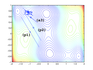
Figure 5.1. The first two iterates of Algorithm 3.3 are operations (PD) to reduce the parallel distance, marked as (p1) and (p2), and the third iterate, marked as (a3), is an (Av) operation to adjust the vector $v$. In this case, the algorithm concentrates its efforts close to the saddle point near $(-1,0.8)$. If a different endpoint had been fixed in (a3) instead, the algorithm might have found the saddle point $(0,0)$. The saddle point $(0,0)$ has a higher value, and would be of greater interest as the bottleneck.

We look at Figure 5.1. One observation that can be made for Algorithm 3.3 is that while Algorithm 3.3 focuses its computations on a saddle point in two runs of (PD) and one run of (Av), it did not focus its computations on the saddle point $(0,0)$, which has a higher critical value. We can see this phenomenon as part of the risks involved in trying to zoom computations to a saddle point. Moreover, this is unavoidable because in a general problem, an optimal mountain pass may be difficult to find by any method. Furthermore, for this example, when the mountain pass algorithm is run between the saddle point near $(-1,0.8)$ and the local minimizer near $(0.1,-0.7)$, it may find the saddle point $(0,0)$.

6. Conclusion

We propose two Principles (P1) and (P2) that a good mountain pass algorithm should satisfy. We proposed the subroutine (PD) in Algorithm 3.1 to build our global mountain pass algorithm in Algorithm 3.3, making use of the parallel distance $g_{l,v}(\cdot)$. Through Proposition 2.1, we see that $g_{l,v}(\cdot)^{2}$ satisfies (P1^′), and that (P2) follows from work in [LP11]. Sections 2 and 4 discuss how $g_{l,v}(\cdot)^{2}$ satisfies property (P1).

Finally, we envision that a robust mountain pass algorithm should include quadratic model methods, level set methods and path-based methods. For example, the points chosen for function and gradient evaluations in a level set method should be such that they provide insight for quadratic model methods and path-based methods. The right blend of these methods allow them to overcome each other’s shortcomings. The evidence from our numerical experiments so far are encouraging.

Acknowledgement.

We thank Jiahao Chen for discussions that led to the main ideas in this paper and for references to the literature on computing saddle points, and to James Renegar for some helpful discussions.

References

- [ABT06] G. Arioli, V. Barutello, and S. Terracini. A new branch of mountain pass solutions for the choreographical 3-body problem. Commun. Math. Phys., 268:439–463, 2006.
- [AR73] A. Ambrosetti and P.H. Rabinowitz. Dual variational methods in critical point theory and applications. J. Funct. Anal., 14:349–381, 1973.
- [CM93] Y.S. Choi and P.J. McKenna. A mountain pass method for the numerical solution of semilinear elliptic equations. Nonlinear Anal., 20:4:417–437, 1993.
- [DCC99] Zhonghai Ding, David Costa, and Goong Chen. A high-linking algorithm for sign-changing solutions of semilinear elliptic equations. Nonlinear Anal., 38:151–172, 1999.
- [Fen94] Y. Feng. The study of nonlinear flexings in a floating beam by variational methods. oscillations in nonlinear systems: Applications and numerical aspects. J. Comput. Appl. Math., 52:1–3:91–112, 1994.
- [GM08] D. Glotov and P.J. McKenna. Numerical mountain pass solutions of Ginzburg-Landau type equations. Comm. Pure Appl. Anal., 7:6:1345–1359, 2008.
- [HJJ00] G. Henkelman, G. Jóhannesson, and H. Jónsson. Methods for finding saddle points and minimum energy paths. In S.D. Schwartz, editor, Progress in Theoretical Chemistry and Physics, pages 269–300. Kluwer, Amsterdam, 2000.
- [HLP06] J. Horák, G.J. Lord, and M.A. Peletier. Cylinder buckling: The mountain pass as an organizing center. SIAM J. Appl. Math., 66:5:1793–1824, 2006.
- [Hor04] J. Horák. Constrained mountain pass algorithm for the numerical solution of semilinear elliptic problems. Numer. Math., 98:251–276, 2004.
- [HS05] H.P. Hratchian and H.B. Schlegel. Finding minima, transition states, and following reaction pathways on ab initio potential energy surfaces. In C.E. Dykstra, K.S. Kim, G. Frenking, and G.E. Scuseria, editors, Theory and Applications of Computational Chemistry: The First 40 Years, pages 195–259. Elsevier, The Netherlands, 2005.
- [Jab03] Youssef Jabri. The Mountain Pass Theorem. Cambridge, 2003.
- [LM91] A.C. Lazer and P.J. McKenna. Nonlinear flexings in a periodically forced floating beam. Math. Method. Appl. Sci., 14:1:1–33, 1991.
- [LP11] A.S. Lewis and C.H.J. Pang. Level set methods for finding critical points of mountain pass type. Nonlinear Anal., 74:12:4058–4082, 2011.
- [LZ01] Yongxin Li and Jianxin Zhou. A minimax method for finding multiple critical points and its applications to semilinear PDEs. SIAM J. Sci. Comput., 23:3:840–865, 2001.
- [MF01] R.A. Miron and K.A. Fichthorn. The step and slide method for finding saddle points on multidimensional potential surfaces. J. Chem. Phys., 115:9:8742–8747, 2001.
- [MM04] J.J. Moré and T.S. Munson. Computing mountain passes and transition states. Math. Program., 100:1:151–182, 2004.
- [MW89] J. Mawhin and M. Willem. Critical point theory and Hamiltonian systems. Springer, New York, 1989.
- [Rab77] P.H. Rabinowitz. Some critical point theorems and applications to semilinear elliptic partial differential equations. Ann. Scuola Norm. Sup. Pisa, 5:412–424, 1977.
- [Rab86] P.H. Rabinowitz. Minimax methods in critical point theory with applications to differential equations. CBMS regional Conf. Ser. in Math, 65, AMS, Providence, RI, 1986.
- [Sch99] M. Schechter. Linking methods in critical point theory. Birkhäuser, Boston, 1999.
- [Sch11] H.B. Schlegel. Geometry optimization. Wiley Interdisciplinary Reviews: Computational Molecular Science, 1:5:790–809, 2011.
- [Str08] M. Struwe. Variational methods. Springer, New York, 4th edition, 2008.
- [Wal03] D.J. Wales. Energy Landscapes: With applications to clusters, biomolecules and glasses. Cambridge, Cambridge, UK, 2003.
- [Wal06] D.J. Wales. Energy landscapes: calculating pathways and rates. International Reviews in Physical Chemistry, 25:1-2:237–282, 2006.
- [Wil96] M. Willem. Minimax theorems. Birkhäuser, Boston, 1996.
- [WZ04] Zhi-Qiang Wang and Jianxin Zhou. A local minimax-Newton’s method for finding critical points with symmetries. SIAM J. Num. Anal., 42:1745–1759, 2004.
- [WZ05] Zhi-Qiang Wang and Jianxin Zhou. An efficient and stable method for computing multiple saddle points with symmetries. SIAM J. Num. Anal., 43:891–907, 2005.
- [YZ05] Xudong Yao and Jianxin Zhou. A local minimax characterization of computing multiple nonsmooth saddle critical points. Math. Program., Ser. B, 104:749–760, 2005.