Occurrence rate of extreme magnetic storms

Abstract

Statistical analysis of occurrence rate of magnetic storms induced by different types of interplanetary drivers is made on the basis of OMNI data for period 1976-2000. Using our catalog of large scale types of solar wind streams we study storms induced by interplanetary coronal mass ejections (ICME) (separately magnetic clouds (MC) and Ejecta) and both types of compressed regions: corotating interaction regions (CIR) and Sheaths. For these types of drivers we calculate integral probabilities of storms with minimum $Dst\leq$ -50, -70, -100, -150, and -200 nT. The highest probability in this interval of Dst is observed for MC, probabilities for other drivers are 3-10 times lower than for MC. Extrapolation of obtained results to extreme storms shows that such a magnetic storm as Carrington storm in 1859 with $Dst=$ -1760 nT is observed on the Earth with frequency 1 event during $\sim$ 500 year.

Gindraft=false YERMOLAEV ET AL. EXTREME MAGNETIC STORMS

1 Introduction

One of the main problems of solar-terrestrial physics and Space Weather is study and prediction of magnetic storms including extreme ones (see, e.g., recent papers and reviews by [Echer et al. (2011), Podladchikova and Petrukovich (2012), Yakovchouk et al. (2012), Yermolaev et al. (2012)] and references therein). Useful technique for problem solution is calculation of frequency (occurrence rate) distributions of events based on observations in form $dN=F(x)dx$, where $dN$ is the number of events recorded with the parameter $x$ of interest between $x$ and $x+dx$, and $F(x)$ is a frequency distributions (see, e.g., recent review and paper by [Crosby (2011), Gorobets and Messerotti (2012)] and references therein). The $Dst$ index (or its proxies) calculated from the observations of the horizontal magnetic field at four low- to mid-latitude ground stations is used to indicate value of magnetic storms (Sugiura, 1964; Sugiura and Kamei, 1991). Recently the geomagnetic storm peak intensity distribution has been obtained for period 1957 to 2008 and it has been described by an exponential form, $F(Dst_{p})=1.2exp(-Dst_{p}/34)$ where $F$ is the probability of geomagnetic storm occurrence with a given value $Dst_{p}$ (Echer et al., 2011). This formula gives too small probability for extreme storms (for instance, for storms such as the 1859 Carrington storm with $Dst=-1760$ nT (Tsurutani et al., 2003) probability is equal to 1 event per 10²³ magnetic storms (Echer et al., 2011) ).

To predict time and value of magnetic storm it is necessary to additionally find relationships between interplanetary and magnetospheric parameters/events. Alves et al. (2011) analyzed interplanetary structures (magnetic clouds with sheath before them – MC, corotating interaction regions – CIR, and shocked plasma) and distributions (histograms and fitting lines) for geomagnetic indices for each interplanetary structure (the geomagnetic indices $Kp(ap)$, $AE$, and $Dst$ are peak values within 2 days after the interplanetary structure has passed near- Earth orbit). The main disadvantages and limitations of this work are following.

1. MC, Ejecta and Sheath events are not selected and analyzed together as ”MC events” though it is well known that these types of interplanetary drivers result in different reaction of magnetosphere (Tsurutani and Gonzalez, 1997; Gonzalez et al., 1999; Yermolaev et al., 2005; Wu and Lepping, 2007; Pulkkinen et al., 2007; Yermolaev et al., 2010c; Kilpua et al., 2012)

2. The used technique of relating of interplanetary driver to magnetic storm is ambiguous because the delay between the reason and its consequence usually does not exceed 2 hours Gonzalez and Echer (2005), and usually duration of interplanetary drivers (average durations 24 $\pm$ 11 h for MC, 29 $\pm$ 5 h for Ejecta, 16 $\pm$ 3 h for Sheath before Ejecta, 9 $\pm$ 5 h for Sheath before MC, and 20 $\pm$ 4 h for CIR (Yermolaev et al., 2007, 2010a)) is less than 2 days.

3. Used approximations at large indices (see Table 4 in paper by Alves et al. (2011)) give constant values 0.06, 0.22 and 0.045 for MC, shock and CIR, respectively, and cannot be used for analysis of extreme storms.

In our previous paper (Yermolaev et al., 2012) we analyzed 798 geomagnetic storms with $Dst\leq-50$ nT and five various types of solar wind streams as their interplanetary sources: corotating interaction regions (CIR), interplanetary coronal mass ejection (ICME) including magnetic clouds (MC) and ejecta, and a compression region sheath before both types of ICME ($SH_{MC}$ and $SH_{Ej}$, respectively) and calculated a probability with which a selected phenomenon can cause a magnetic storm, i.e., the ratio between the number of events $K_{j}$ of a chosen stream type $j$ (MC, CIR etc.) resulting in a magnetic storm with $Dst<Dst_{0}$ and the total number of this type events $N_{j}$: $P_{j}=K_{j}/N_{j}$. In contrast with papers by Alves et al. (2011) and Echer et al. (2011) we calculated an integral probability summing probabilities from $-\infty$ up to $Dst_{0}$, i.e. $P_{j}(Dst_{0})=\int_{-\infty}^{Dst_{0}}F_{j}(Dst)d(Dst)$. In previous paper we calculated $P(-50)$ for MC, Ejecta, Sheath and CIR. In this paper we calculate integral probabilities for $|Dst|=50,70,100,150,200$ nT and extrapolate them to stronger, extreme storms with $|Dst|=500,1000,1700$ nT.

2 Methods

We use our catalog of large-scale solar wind phenomena in 1976–2000 (see ftp://www.iki.rssi.ru/pub/omni (Yermolaev et al., 2009) obtained on the basis of OMNI database (see http://omniweb.gsfc.nasa.gov (King and Papitashvili, 2004) and data on $Dst$ index (see http://wdc.kugi.kyoto-u.ac.jp/index.html). The technique of determination of connection between magnetic storms and their interplanetary drivers consists in the following. If the minimum of $Dst$ index lies in an interval of a type of solar wind streams or is observed within 1–2 hours after it we believe that the given storm has been generated by the given type of streams (Yermolaev et al., 2010). During 1976-200 there were 798 magnetic storms with minimum $Dst\leq$ -50 nT but the source of 334 magnetic storms (i.e., 42 % of 798 storms) occurred to be undetermined, mainly because of the absence of a complete set of measurements for separate time intervals in the OMNI database.

We use indicated data to calculate following parameters: (1) integral probability $P_{j}(Dst_{0})$ and (2) waiting time $T_{j}(Dst_{0})$. $P_{j}(Dst_{0})=K_{j}(Dst_{0})/N_{j}$, where $N_{j}$ is total number of solar wind events of type $j$ observed during period 1976-2000, $K_{j}(Dst_{0})$ is number of solar wind events of type $j$ induced magnetic storms with minimum $Dst\leq Dst_{0}$, i.e. $P_{j}(Dst_{0})$ is function of threshold $Dst_{0}$. In this work we calculate integral probability for values $Dst_{0}$ = -50, -70, -100, -150, and -200 nT and for 4 types of interplanetary drivers ( CIR, Sheath, MC, Ejecta as well as ME=MC+Ejecta) on the basis of experimental data. These experimental points are approximated by different functions and obtained approximations allows us to extrapolate probabilities to extreme magnetic storms with high values $Dst_{0}$ = -500, -1000, and -1700 nT for which experimental data are too scare to calculate real probabilities.

An important parameter of magnetic storms is a waiting time which is average period between consecutive observations of magnetic storms stronger $Dst_{0}$ generated by solar wind type $j$, i.e. $T_{j}(Dst_{0})=[P_{j}(Dst_{0})N_{j}/(t*r)]^{-1}$, where $t$ = 26 years (duration of observations from 1976 up to 2000) and $r$ = 0.58 (ratio of durations of data existence to total duration of observation). To estimate waiting times $T_{j}(Dst_{0})$ for $Dst_{0}$ = -500, -1000, and -1700 nT, we use approximating functions pf integral probabilities at these values of $Dst$ index.

3 Results

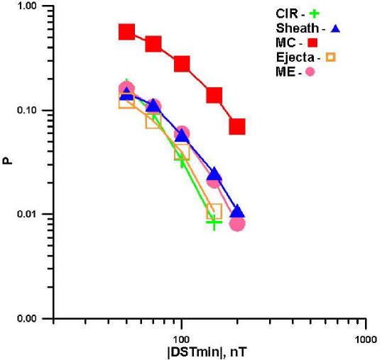
Figure 1: Dependence of integral probability $P_{j}(|Dst|>Dst_{0})$ on the value of storm for different types of solar wind.

Total numbers of different interplanetary drivers $N_{j}$, numbers of drivers resulting in magnetic storms $K_{j}(Dst_{0})$ and integral probabilities $P_{j}(Dst_{0})$ for $|Dst_{0}|=50,70,100,150,200$ nT are presented in Table 1. Data in last column with $K_{j}(-200)=$ 3 and 5 for CIR and Ejecta were excluded from consideration of $P_{j}$ because of too low statistics. Obtained data on $P_{j}$ are presented in Figure 1.

These data shows that the highest probability is observed for magnetic clouds. At $Dst_{0}$ index increase from 50 to the 200 nT the probability fell almost in 10 times. The probability for other types is less in 3-4 times at $|Dst_{0}|$ = 50 and 5-15 times at 200 nT, i.e. the probability for magnetic clouds decreases more slowly with increasing index than for other drives. It is important to note that ratio of probabilities of MC and Ejecta changes from 5 at $|Dst_{0}|$ = 50 nT upto 10 at $|Dst_{0}|$ = 150 nT and probability of ICME (indicated as ME = MC + Ejecta) is close to probability of Ejecta, and this fact is serious argument to analyze MC and Ejecta separately.

4 Discussion

Obtained results allow us to calculate probabilities and waiting times of magnetic storms in $Dst$ range from -50 down to - 200 nT for various interplanetary drivers and to use these parameters for forecasting of magnetic storms. Unfortunately, there is no enough number of events to calculate these parameters for larger storms. Nevertheless obtained data can be approximated by functions and these approximations can be used for extrapolation of probabilities in range of very large storms.

In accordance with paper by Crosby (2011) various events on the Sun and the Earth have similar shape of distributions: a top at small values, then a gentle slop and power–law tail at large values. If suggestion on power–law distribution at given values of $Dst$ is true, obtained data can be approximated by power–law functions and these approximations were made using last highest 3 measured points of $|Dst|$ (see Table 2 and thing lines in figure 2). As seen in Fig.2, dependence of $log(P)$ on $log(|Dst|)$ is not linear (as it should be for power law). So we made square approximation in log-log scales (see Table 2 and thick lines in figure 2). The square-law dependencies are too steeply decreasing and do not agree conclusion by Crosby (2011) about power–low tail at large values. We suggest that dependencies do not approach power–law part of distribution in range of $|Dst_{0}|=50,70,100,150,200$. So, we take power law with fixed index -2.5 for MC (see Table 2 and dashed line in figure 2) and believe that this line is the best approximation. The probabilities for another drivers in these range of $Dst$ have been approximated by power law with fixed index -2.5 (not shown) and obtained lines look better than power–law fittings on last 3 points and square–law fittings.

Probabilities obtained by extrapolations of fittings are used for calculation of waiting times for extreme storms with minimum $Dst\leq$ -500, -1000, and -1700 nT (see Table 2). The data spread is very large but it is possible to make some rough estimations. The least waiting times (e.g. the highest probability) is observed for MC. Other drivers have larger waiting times (lower probabilities) and their contribution can be neglected. Thus, the most probable estimations of waiting times for extreme magnetic storms with minimum $Dst\leq$ -500, -1000, and -1700 nT are $\sim$20, $\sim$100 and $\sim$500 years (with accuracy of factors $\sim$1.5, $\sim$2, and $\sim$3), respectively. It should be noted that we use 26 year observations to estimate waiting time of 100 and 500 years, therefore accuracy of estimates is very low. Nevertheless the obtained estimates appear more realistic than ones were obtained by Echer et al. (2011). In order essentially to increase accuracy and reliability of estimates by means of this technique it is necessary to increase duration of an interval of observation several times.

5 Conclusions

On the basis of OMNI dataset during 1976-2000 we classified different types of solar wind events (magnetic cloud MC, Ejecta, CIR, and Sheath), found magnetic storms corresponding to these types of interplanetary drivers and calculated integral probabilities of generation of magnetic storms with minimum $Dst\leq$ -50, -70, -100, -150 and -200 nT by these types of solar wind drivers. Obtained data allow one to make following conclusions.

1. Probabilities of storm generation by all types of drivers decrease with decreasing minimum $Dst$ index, and rate of probability decrease increases with index decreasing.

2. Probability for MC is the highest one, and rate of its probability decrease is the smallest.

3. Probabilities of CIR–, Ejecta– and Sheath–induced storms with $Dst\leq$ -50 nT are less in 3-4 times than for MC, for storms with $Dst\leq$ -200 nT their probabilities are less in 5-15 times.

Interpolation of data in $Dst$ region from -50 down to -200 nT and than extrapolation for stronger, extreme storms with $Dst\leq$ -500, -1000, and -1700 nT allow us to suggest the following.

1. The most probable estimations of waiting times for extreme magnetic storms with minimum $Dst\leq$ -500, -1000, and -1700 nT are $\sim$20, $\sim$100 and $\sim$500 years (with accuracy of factors $\sim$1.5, $\sim$2, and $\sim$3), respectively.

2. The waiting times of CIR–, Ejecta– and Sheath–induced storms with $Dst\leq$ -500 nT are larger in 5-10 times than for MC, their waiting times for storms with $Dst\leq$ -1700 nT are larger in 10-100 times than for MC. Therefore their waiting times for extreme storms is very small relative to MC one and their contribution in extreme storm generation can be neglected.

Obtained experimental results and estimations are important for space weather and, in particular, for analysis and forecasting of extreme magnetic storms.

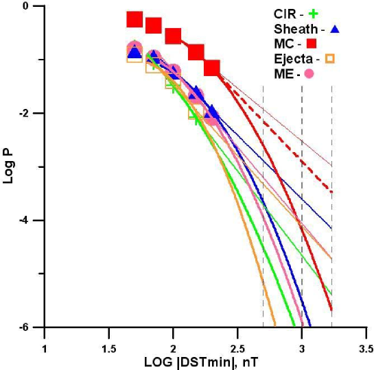
Figure 2: Approximations of dependence of integral probability $P(|Dst|>Dst0)$ on the value of storm for different types of solar wind. Vertical dashed lines show 500, 1000 and 1700 nT.

Table 1: Probabilities $P_{j}$ generation of magnetic storms with $Dst\leq$ -50, -70, -100, -150 and -200 nT for different types of interplanetary drivers.

Types of	Number,	$Dst\leq-50$		$Dst\leq-70$		$Dst\leq-100$		$Dst\leq-150$		$Dst\leq-200$
drivers	$N_{j}$	$K_{j}$	$P_{j}$	$K_{j}$	$P_{j}$	$K_{j}$	$P_{j}$	$K_{j}$	$P_{j}$	$K_{j}$	$P_{j}$
CIR	718	120	0.167	66	9.2 $10^{-2}$	24	3.3 $10^{-2}$	6	8.4 $10^{-3}$	5	-
Sheath	642	93	0.145	72	0.112	37	5.8 $10^{-2}$	16	2.6 $10^{-2}$	7	1.1 $10^{-2}$
MC	101	57	0.564	44	0.436	28	0.227	14	0.139	7	6.9 $10^{-2}$
Ejecta	1127	139	0.123	89	7.9 $10^{-2}$	45	4.0 $10^{-2}$	12	1.1 $10^{-2}$	3	-
ME (MC + Ejecta)	1228	196	0.159	133	0.108	73	5.9 $10^{-2}$	26	2.1 $10^{-2}$	10	8.1 $10^{-3}$

Table 2: Approximations of integral probabilities $P_{j}$ and waiting times (average occurrence periods) $T_{j}$ for magnetic storms with $|Dst|>500,1000,1700$ nT.

Types of	Extrapolation,	$|Dst|>500$		$|Dst|>1000$		$|Dst|>1700$
drivers	$Y=log(P),X=log(|Dst|)$	$P$	$T$	$P$	$T$	$P$	$T$
MC	$Y=-1.98X+7.87$	11.18 $10^{-2}$	12.7	2.99 $10^{-3}$	50	1.05 $10^{-3}$	142
	$Y=-2.5X+4.6$	7.12 $10^{-3}$	21.0	1.26 $10^{-3}$	118	3.34 $10^{-4}$	447
	$Y=-4.19+5.14X-1.66X^{2}$	3.87 $10^{-3}$	38.6	1.93 $10^{-4}$	774	$1.2210^{-5}$	12200
Ejecta	$Y=-3.26X+5.12$	2.10 $10^{-4}$	63.7	2.20 $10^{-5}$	608	$3.8910^{-6}$	3400
	$Y=-8.73+9.91X-3.13X^{2}$	1.74 $10^{-5}$	770	7.23 $10^{-8}$	1.9 $10^{5}$	$4.4910^{-10}$	3.0 $10^{7}$
ME	$Y=-2.85X+4.48$	6.31 $10^{-4}$	19.5	8.77 $10^{-5}$	140	$1.9410^{-5}$	630
	$Y=-6.39+7.30X-2.36X^{2}$	1.34 $10^{-4}$	91.6	1.90 $10^{-6}$	6500	$3.7510^{-8}$	3.3 $10^{5}$
CIR	$Y=-3.42X+5.36$	1.36 $10^{-4}$	154	1.27 $10^{-5}$	1650	$2.0810^{-6}$	10100
	$Y=-5.51+7.11X-2.54X^{2}$	1.42 $10^{-5}$	1480	8.53 $10^{-8}$	2.5 $10^{5}$	8.28 $10^{-10}$	2.5 $10^{7}$
Sheath	$Y=-2.38X+3.54$	1.30 $10^{-3}$	18.1	2.49 $10^{-4}$	94.3	7.05 $10^{-5}$	333
	$Y=-5.35+6.01X-1.97X^{2}$	3.19 $10^{-4}$	73.6	8.50 $10^{-6}$	2760	3,03 $10^{-7}$	7.8 $10^{4}$