Dynamical Decoupling in Common Environment

Abstract

Dynamical decoupling (DD) sequences were invented to eliminate the direct coupling between qubit and its environment. We further investigate the possibility of decoupling the indirect qubit-qubit interaction induced by a common environment, and sucessfully find simplified solutions that preserve the bipartite quantum states to arbitrary order. Through analyzing the exact dynamics of the controlled two-qubit density matrix, we have proven that applying independent Uhrig Dynamical Decoupling (UDD) on each qubit will effectively eliminate both the qubit-environment and indirect qubit-qubit coupling to the same order as in single qubit case, only if orders of the two UDD sequences have different parity. More specifically, UDD($n$) on one qubit with UDD($m$) on another are able to produce $\min(n,m)$th order suppression while $n+m$ is odd. Our results can be used to reduce the pulse number in relevant experiments for protecting bipartite quantum states, or dynamically manipulate the indirect interaction within certain quantum gate and quantum bus.

1 Introduction

Qubit is constantly losing its coherence due to interaction with environment. Dynamical decoupling sequences are proposed to eliminate the unwanted qubit-environment couplings with instantaneous $\pi$ pulses, and efficiency of DD sequences is largely dependent on the pulse locations. Equidistant DD is a first order solution [1], while more advanced sequences employ non-equidistant [2, 3] or concatenated pulse locations [4, 5]. Particularly in this article we are concerned about UDD [2], whose pulse locations are $t\delta_{j}$

$$\delta_{j}=\sin^{2}(j\pi/2(n+1)).$$

UDD sequence was first derived under pure dephasing models [6], able to protect the qubit coherence up to $n$th order with $n$ pulses.

In recent years, DD has been successfully extended to preserve multipartite quantum states [7, 8, 9, 10, 11, 12, 13]. By nesting layers of UDD (NUDD), total $(n+1)^{m}$ pulses are needed to freeze a system of $m$ qubits to $n$th order without knowing any details of the qubit-environment coupling [8, 10, 14, 15, 16]. It can be seen that in NUDD pulse number grows polynomial with pulse order. However for a specific experimental setup, it is more realistic and efficient to tailor the pulse sequence accordingly, since pulse number is limited during a fixed time interval [17, 18] and errors from each imperfect pulse will accumulate [19, 20, 21]. There are already some efforts to reduce the pulse number. If prior knowledge is available, such as initial qubit state [7], environmental coupling spectrum [11] or unbalanced decoherence rates [12], the above universal plan can be greatly simplified.

In this paper we introduce another approach to reduce the DD sequence which is needed for a two-qubit system linearly coupled to a common bosonic bath. This situation may arise when two qubits are not spatially separated enough to create independent environments [22], or noises felt by each qubit are correlated [11, 23]. In addition, common environment has long been exploited to generate entangling gate and serve as quantum bus between qubits [24, 25, 26, 27]. While these gates and buses are idle we can use DD sequences to switch off the interactions and in the meantime protect the states.

As it turns out, the simplified sequence is made very easy to implement. For example, we can apply UDD($n$) ($n$-pulse UDD) on first qubit and UDD($m$) on second qubit. $n$ and $m$ can be chosen at will as long as they have different parity. The whole sequence will preserve the bipartite state up to an order of $\min(n,m)$. For $m=n+1$, this scheme only needs $2n+1$ pulses, while NUDD($n$) needs $(n+1)^{2}$.

We organize this paper as follows. In Sec. II we discuss the free dynamics of a two-qubit system in a common bosonic bath. In Sec. III, controlled dynamics and conditions for high-level DD are derived. Sequences satisfying these conditions are given. Conclusions are put in Sec. IV.

2 Dynamics in Common Quantum Bath

We consider a two-qubit spin-boson model:

$$H=\sum_{k}\omega_{k}b_{k}^{\dagger}b_{k}+(\sigma_{z_{1}}+\sigma_{z_{2}})\sum_{k}\lambda_{k}(b_{k}^{\dagger}+b_{k}),$$ (1)

where $b_{k}$ is the annihilation operator for the $k$th mode of the bath and $\lambda_{k}$ is coupling strength. $\sigma_{z_{1}}$ and $\sigma_{z_{2}}$ are spin operators acting on first and second qubit respectively. This model describes a pure dephasing process due to the couplings with environment. With $|\uparrow\rangle$ and $|\downarrow\rangle$ being the eigenstates of $\sigma_{z}$, we can define four basis states $|0\rangle=|\downarrow\downarrow\rangle,|1\rangle=|\downarrow\uparrow\rangle,|2\rangle=|\uparrow\downarrow\rangle,|3\rangle=|\uparrow\uparrow\rangle$ for a bipartite quantum state.

The dynamics of Eq. ($1$) can be exactly solved [25, 28]. In the interaction picture of the bath operator $\sum_{k}\omega_{k}b_{k}^{\dagger}b_{k}$, the unitary evolution that generated by the time-dependent interaction Hamiltonian can be computed using Magnus expansion. It is easy to verify that only the first two terms of the expansion are nonzero (see [28] for more details). As a result, the free evolution of the composite system can be calculated as follows

$$U_{f}(t) = \exp[(\sigma_{z_{1}}+\sigma_{z_{2}})\sum_{k}\lambda_{k}(\frac{e^{-\mbox{i}\omega_{k}t}-1}{\omega_{k}}b_{k}-\frac{e^{\mbox{i}\omega_{k}t}-1}{\omega_{k}}b_{k}^{\dagger})$$ (2)

$$+ \mbox{i}(\sigma_{z_{1}}+\sigma_{z_{2}})^{2}\sum_{k}\lambda_{k}^{2}\frac{\omega_{k}t-\sin\omega_{k}t}{\omega_{k}^{2}}].$$

The collective term $(\sigma_{z_{1}}+\sigma_{z_{2}})^{2}=2(I+\sigma_{z_{1}}\sigma_{z_{2}})$ generates an indirect coupling between the two qubits dependent on their states, which will further induce an oscillation of quantum correlations [25, 27, 29]. In order to preserve an arbitrary state, not only couplings to bath oscillators but also the indirect couplings must be removed. By introducing the spectral density function [30] defined as $J(\omega)=\sum_{k}\lambda_{k}^{2}\delta(\omega-\omega_{k})$, we can then write down the evolution of the density matrix $\rho(t)$

$$\left(\begin{array}[]{cccc}1&{e^{\mbox{i}\Delta(t)-\Gamma(t)}}&{e^{\mbox{i}\Delta(t)-\Gamma(t)}}&{e^{-4\Gamma(t)}}\\ {e^{-\mbox{i}\Delta(t)-\Gamma(t)}}&1&1&{e^{-\mbox{i}\Delta(t)-\Gamma(t)}}\\ {e^{-\mbox{i}\Delta(t)-\Gamma(t)}}&1&1&{e^{-\mbox{i}\Delta(t)-\Gamma(t)}}\\ {e^{-4\Gamma(t)}}&{e^{\mbox{i}\Delta(t)-\Gamma(t)}}&{e^{\mbox{i}\Delta(t)-\Gamma(t)}}&1\end{array}\right),$$

with

$$\Delta(t) = 4\int_{0}^{\infty}J(\omega)\frac{\omega{t}-\sin\omega{t}}{\omega^{2}}d\omega,$$ (3)

$$\Gamma(t) = 4\int_{0}^{\infty}J(\omega)\frac{2\sin^{2}(\omega{t}/2)}{\omega^{2}}\coth(\frac{\beta\omega}{2})d\omega.$$ (4)

$\beta$ is the inverse temperature. The exponentially decaying factor $\Gamma(t)$ is associated with decoherence process, while $\Delta(t)$ represents collective phase evolution. Note that the phase factor is absent in classical noise model [11, 23]. If two qubits are subjected to the same classical noise, it is adequate to use simultaneous DD pulses on each qubit.

In the case of quantum noise, still by flipping the sign of $\sigma_{z_{1}}$ and $\sigma_{z_{2}}$ with $\pi$ pulses, $\Gamma(t)$ will be effectively averaged to zero. However, we cannot apply the same sequence on both qubits, since simultaneous $\pi$ pulses will have no influence on the value of $(\sigma_{z_{1}}+\sigma_{z_{2}})^{2}$ and so on phase evolution. This motivates us to consider the following scenario: $n$ pulses of $\pi$ rotation along axis-$x$ are applied to the first qubit, with the pulse locations given by $\delta_{1^{{}^{\prime}}},\delta_{2^{{}^{\prime}}},...,\delta_{n^{{}^{\prime}}}$, whereas $m$ analogous pulses are applied to the second qubit at different times $\delta_{1^{{}^{\prime\prime}}},\delta_{2^{{}^{\prime\prime}}},...,\delta_{{m}^{{}^{\prime\prime}}}$. Totally $n+m$ pulses are applied to the two-qubit system. We arrange the $n+m$ pulse timings in increasing order and denote them by $\delta_{1},\delta_{2},...,\delta_{n+m}$, with $\delta_{j}<\delta_{j+1}$. At each $\delta_{j}$, either the $\sigma_{z_{1}}$ or $\sigma_{z_{2}}$ operator switches its sign. At the same time, the operator $\sigma_{z_{1}}\sigma_{z_{2}}$ changes its sign $n+m$ times at these instants. In the next section we seek to find the correct $n+m$ pulse locations which preserve both phases and amplitudes of the density matrix elements.

3 Pulse Controlled Dynamics

In this section we adopt the canonical transformation technique which was used in deriving the UDD sequence for single qubit [2, 6]. Also we use the notations from [6] by defining

$$A^{\mbox{eff}} = UAU^{\dagger},A(t)=\exp(\mbox{i}H^{\mbox{eff}}t)A\exp(-\mbox{i}H^{\mbox{eff}}t),$$ (5)

$$U = \exp[(\sigma_{z_{1}}+\sigma_{z_{2}})K],K=\sum_{k}\frac{\lambda_{k}}{\omega_{k}}(b_{k}^{\dagger}-b_{k}).$$ (6)

Operator $A^{\mbox{eff}}$ acquires time dependence under the action of the “effective” Hamiltonian. After the canonical transformation $U$, the effective Hamiltonian is diagonal

$$H^{\mbox{eff}}=\sum_{k}\omega_{k}b_{k}^{\dagger}b_{k}-\frac{\lambda_{k}^{2}}{\omega_{k}}(\sigma_{z_{1}}+\sigma_{z_{2}})^{2}$$ (7)

and the time-dependent flip operators $\sigma_{x_{i}}^{\mbox{eff}}(t)$ are

$$\sigma_{x_{i}}^{\mbox{eff}}(t)=\exp[2\sigma_{z_{i}}K(t)]\exp(-4\mbox{i}\sum_{k}\frac{\lambda_{k}^{2}}{\omega_{k}}\sigma_{z_{1}}\sigma_{z_{2}}t)\sigma_{x_{i}},$$ (8)

with

$$K(t)=\sum_{k}\frac{\lambda_{k}}{\omega_{k}}(b_{k}^{\dagger}e^{\mbox{i}\omega_{k}t}-b_{k}e^{-\mbox{i}\omega_{k}t}).$$ (9)

Making use of these expressions, dynamics of the density matrix elements can be obtained by explicit calculation. For an arbitrary element $\rho_{SS^{{}^{\prime}}}$, the average evolution is

$$\langle{\langle}S|e^{\mbox{i}Ht}|S\rangle{\langle}S^{{}^{\prime}}|e^{-\mbox{i}Ht}|S^{{}^{\prime}}\rangle\rangle$$

$$=\langle{\langle}S|e^{\mbox{i}H(\delta_{1}-\delta_{0})t}\sigma_{x_{j_{1}}}e^{\mbox{i}H(\delta_{2}-\delta_{1})t}...e^{\mbox{i}H(\delta_{n+m}-\delta_{n+m-1})t}\sigma_{x_{j_{n+m}}}e^{\mbox{i}H(\delta_{n+m+1}-\delta_{n+m})t}(\sigma_{x_{i}})|S\rangle$$

$${\langle}S^{{}^{\prime}}|(\sigma_{x_{i}})e^{-\mbox{i}H(\delta_{n+m+1}-\delta_{n+m})t}\sigma_{x_{j_{n+m}}}e^{-\mbox{i}H(\delta_{n+m}-\delta_{n+m-1})t}...e^{-\mbox{i}H(\delta_{2}-\delta_{1})t}\sigma_{x_{j_{1}}}e^{-\mbox{i}H(\delta_{1}-\delta_{0})t}|S^{{}^{\prime}}\rangle\rangle$$

$$=\langle{\langle}S|U^{\dagger}\sigma_{x_{j_{1}}}(\delta_{1}t)\sigma_{x_{j_{2}}}(\delta_{2}t)...\sigma_{x_{j_{n+m-1}}}(\delta_{n+m-1}t)\sigma_{x_{j_{n+m}}}(\delta_{n+m}t)(\sigma_{x_{i}}^{\mbox{eff}}(t))e^{\mbox{i}H^{\mbox{eff}}t}U|S\rangle$$

$${\langle}S^{{}^{\prime}}|U^{\dagger}e^{-\mbox{i}H^{\mbox{eff}}t}(\sigma_{x_{i}}^{\mbox{eff}}(t))\sigma_{x_{j_{n+m}}}(\delta_{n+m}t)\sigma_{x_{j_{n+m-1}}}(\delta_{n+m-1}t)...\sigma_{x_{j_{2}}}(\delta_{2}t)\sigma_{x_{j_{1}}}(\delta_{1}t)U|S^{{}^{\prime}}\rangle\rangle$$

$$=\langle{\langle}S|U^{\dagger}\sigma_{x_{j_{1}}}(\delta_{1}t)\sigma_{x_{j_{2}}}(\delta_{2}t)...\sigma_{x_{j_{n+m-1}}}(\delta_{n+m-1}t)\sigma_{x_{j_{n+m}}}(\delta_{n+m}t)(\sigma_{x_{i}}^{\mbox{eff}}(t))$$

$$e^{(s_{1}-s_{2})K(t)}e^{-\mbox{i}\sum_{k}\frac{\lambda_{k}^{2}}{\omega_{k}}({s_{1}}^{2}-{s_{2}}^{2})t}|S\rangle{\langle}S^{{}^{\prime}}|(\sigma_{x_{i}}^{\mbox{eff}}(t))\sigma_{x_{j_{n+m}}}(\delta_{n+m}t)$$

$$\sigma_{x_{j_{n+m-1}}}(\delta_{n+m-1}t)...\sigma_{x_{j_{2}}}(\delta_{2}t)\sigma_{x_{j_{1}}}(\delta_{1}t)U|S^{{}^{\prime}}\rangle\rangle.$$ (10)

$s_{1},s_{2}$ are eigenvalues of $\sigma_{z_{1}}+\sigma_{z_{2}}$ for $|S\rangle$ and $|S^{{}^{\prime}}\rangle$. Determined by which spin is flipped at $\delta_{j}$, $j_{1},j_{2},...j_{n+m}$ take values from $\{1,2\}$. By $(\sigma_{x_{i}})$ we mean that an ending pulse $\sigma_{x_{i}}$ is added at the end of the sequence to ensure the final state is still $|S\rangle{\langle}S^{{}^{\prime}}|$ if $n+m$ is odd (If $n$ and $m$ are both odd, two ending pulses are needed). However according to our calculation, whether or not there is an (or two) ending pulse will not modify the equations and results we derive next. The outermost brackets denote ensemble average with respect to the thermal bath.

The sum of all terms in the form of $-4\mbox{i}\sum_{k}(\lambda_{k}^{2}/\omega_{k})\sigma_{z_{1}}\sigma_{z_{2}}$ from Eq. ($10$) leads to a phase shift

$$\exp[-4\mbox{i}\sum_{k}\frac{\lambda_{k}^{2}}{\omega_{k}}(s_{1}-s_{2})(\delta_{1}-\delta_{2}+...+(-1)^{n+m-1}\delta_{n+m}+\frac{(-1)^{n+m}}{2})t],$$

and calculation of the rest part of Eq. ($10$) will produce more phases. Taking $\rho_{01}(t)$ as an example, we are left with

$${\langle}e^{2K}e^{-2K(\delta_{1}t)}e^{(\pm)2K(\delta_{2}t)}...e^{(\pm)2K(\delta_{m+n}t)}e^{(-1)^{m+1}2K(t)}$$

$$e^{(\pm)2K(\delta_{m+n}t)}...e^{(\pm)2K(\delta_{2}t)}e^{-2K(\delta_{1}t)}\rangle.$$

Coefficients before each $K(\delta_{i}t)$ are determined by the relative locations between 1st-qubit and 2nd-qubit pulses in the whole sequence. Exponentials in Eq. ($12$) can be combined one by one using Baker-Campbell-Hausdorff formula $e^{A}e^{B}=e^{A+B}e^{[A,B]/2}$, which is valid here because

$$[K(t),K(t^{{}^{\prime}})]=2\mbox{i}\sum_{k}(\lambda_{k}^{2}/\omega_{k}^{2})\sin\omega_{k}(t-t^{{}^{\prime}})$$

is a $c$-number. After the combination all $K(\delta_{i}t)$ add up to one exponential $\exp[-2K(\delta_{1^{{}^{\prime\prime}}}t)+2K(\delta_{2^{{}^{\prime\prime}}}t)...+(-1)^{m}2K(\delta_{m^{{}^{\prime\prime}}}t)+(-1)^{m+1}2K(t)+(-1)^{m}2K(\delta_{m^{{}^{\prime\prime}}}t)...+2K(\delta_{2^{{}^{\prime\prime}}}t)-2K(\delta_{1^{{}^{\prime\prime}}}t)]$ while extra phases introduced by the $e^{[A,B]/2}$ term in Hausdorff formula can be calculated by observing that combining any four symmetric exponentials $e^{\pm 2K(\delta_{p}t)}$ and $e^{\pm 2K(\delta_{q}t)}$ on both sides of $e^{(-1)^{m+1}2K(t)}$ will not create extra phases except for one case: that is when combine $e^{(-1)^{i}2K(\delta_{i^{{}^{\prime}}}t)}$ with the exponentials which act on the 2nd qubit after it

$$e^{(-1)^{i}2K(\delta_{i^{{}^{\prime}}}t)}e^{(-1)^{j}2K(\delta_{j^{{}^{\prime\prime}}}t)}e^{(-1)^{j}2K(\delta_{j^{{}^{\prime\prime}}}t)}e^{(-1)^{i}(-2)K(\delta_{i^{{}^{\prime}}}t)}$$

$$=e^{(-1)^{i+j}16\mbox{i}\sum_{k}\frac{\lambda_{k}^{2}}{\omega_{k}^{2}}\sin\omega_{k}(\delta_{i^{{}^{\prime}}}-\delta_{j^{{}^{\prime\prime}}})t}e^{(-1)^{j}4K(\delta_{j^{{}^{\prime\prime}}}t)},(i^{{}^{\prime}}<j^{{}^{\prime\prime}}).$$

Merging these exponentials four by four, we arrive at

$$\exp\{\mbox{i}\sum_{k}\frac{\lambda_{k}^{2}}{\omega_{k}^{2}}[8\sum_{i=1}^{n}(-1)^{i+m+1}\sin\omega_{k}(\delta_{i^{{}^{\prime}}}-1)t$$

$$+16\sum_{i=1}^{n}\sum_{i^{{}^{\prime}}<j^{{}^{\prime\prime}}}^{m}(-1)^{i+j}\sin\omega_{k}(\delta_{i^{{}^{\prime}}}-\delta_{j^{{}^{\prime\prime}}})t]\}$$

$${\langle}\exp(2K)\exp[-2K(\delta_{1^{{}^{\prime\prime}}}t)+2K(\delta_{2^{{}^{\prime\prime}}}t)...$$

$$+(-1)^{m}2K(\delta_{m^{{}^{\prime\prime}}}t)+(-1)^{m+1}2K(t)+(-1)^{m}2K(\delta_{m^{{}^{\prime\prime}}}t)$$

$$...+2K(\delta_{2^{{}^{\prime\prime}}}t)-2K(\delta_{1^{{}^{\prime\prime}}}t)]\rangle.$$ (14)

The ensemble average in Eq. ($14$) has already been calculated in [6]. With the existing results from [6] and combining Eq. ($11$) and Eq. ($14$), the final form of $\rho_{01}(t)$ can be organized in a rather compact way

$$\rho_{01}(t)=\exp(\mbox{i}\Delta_{m}(t)-\Gamma_{m}(t)),$$ (15)

with

$$\Delta_{m}(t) = 4\int_{0}^{\infty}\frac{J(\omega)}{\omega^{2}}(x_{m}+z_{m}+c)(\omega{t})d\omega,$$

$$\Gamma_{m}(t) = 2\int_{0}^{\infty}J(\omega)\frac{|y_{m}(\omega{t})|^{2}}{\omega^{2}}\coth(\beta\omega/2)d\omega,$$

$$x_{m}(\omega{t}) = (-1)^{m}\sin(\omega{t})+2\sum_{j=1}^{m}(-1)^{j+1}\sin(\omega{t}\delta_{j^{{}^{\prime\prime}}}),$$

$$y_{m}(\omega{t}) = 1+(-1)^{m+1}e^{\mbox{i}\omega{t}}+2\sum_{j=1}^{m}(-1)^{j}e^{\mbox{i}\omega{t}\delta_{j^{{}^{\prime\prime}}}},$$

$$z_{m}(\omega{t}) = 2\sum_{i=1}^{n}(-1)^{i+m+1}\sin\omega{t}(\delta_{i^{{}^{\prime}}}-1)+4\sum_{i=1}^{n}\sum_{i^{{}^{\prime}}<j^{{}^{\prime\prime}}}^{m}(-1)^{i+j}\sin\omega{t}(\delta_{i^{{}^{\prime}}}-\delta_{j^{{}^{\prime\prime}}}),$$

$$c(\omega{t}) = -2\omega{t}[\sum_{r}^{n+m}(-1)^{r-1}\delta_{r}+\frac{(-1)^{n+m}}{2}].$$ (16)

Unlike single qubit DD, here the phase factor $\Delta_{m}(t)$ will induce collective dynamics and should be minimized. $y_{m}(\omega{t})$ is the so-called filter function of an $m$-pulse sequence [2, 3] and $\Gamma_{m}(t)$ is responsible for decoherence.

The most simple way to realize dynamical decoupling is to use independent UDD sequences to suppress the decoherence, and hope that phase evolutions will be minimized automatically at the same time. UDD($m$) requires the first $m$ derivatives of the filter function to be zero at $\omega=0$. These constraints are imposed to engineer $y_{m}(\omega{t})$ in low frequency region, achieving an error order of $O(t^{m})$. Similarly we can also define the filter function for $\Delta_{m}(t)$ as

$$f_{m}(\omega{t})=x_{m}(\omega{t})+z_{m}(\omega{t})+c(\omega{t}).$$ (17)

The density matrix $\rho(t)$ that controlled by an arbitrary pulse sequence reads

$$\left(\begin{array}[]{cccc}1&{e^{\mbox{i}\Delta_{m}(t)-\Gamma_{m}(t)}}&{e^{\mbox{i}\Delta_{n}(t)-\Gamma_{n}(t)}}&{e^{-\Gamma_{n}(t)-\Gamma_{m}(t)-\gamma(t)}}\\ {e^{-\mbox{i}\Delta_{m}(t)-\Gamma_{m}(t)}}&1&{e^{-\Gamma_{n}(t)-\Gamma_{m}(t)-\gamma(t)}}&{e^{-\mbox{i}\Delta_{n}(t)-\Gamma_{n}(t)}}\\ {e^{-\mbox{i}\Delta_{n}(t)-\Gamma_{n}(t)}}&{e^{-\Gamma_{n}(t)-\Gamma_{m}(t)-\gamma(t)}}&1&{e^{-\mbox{i}\Delta_{m}(t)-\Gamma_{m}(t)}}\\ {e^{-\Gamma_{n}(t)-\Gamma_{m}(t)-\gamma(t)}}&{e^{\mbox{i}\Delta_{n}(t)-\Gamma_{n}(t)}}&{e^{\mbox{i}\Delta_{m}(t)-\Gamma_{m}(t)}}&1\end{array}\right),$$

with

$$\gamma(t)=4\int_{0}^{\infty}\frac{J(\omega)}{\omega^{2}}\Re(y_{n}(\omega{t})y_{m}^{*}(\omega{t}))\coth(\beta\omega/2)d\omega.$$ (18)

Definitions of $\Delta_{n}(t)$ and $\Gamma_{n}(t)$ are the same as Eq. ($16$), but with pulse locations swapped. For example,

$$z_{n}(\omega{t}) = 2\sum_{j=1}^{m}(-1)^{j+n+1}\sin\omega{t}(\delta_{j^{{}^{\prime\prime}}}-1)$$ (19)

$$+ 4\sum_{j=1}^{m}\sum_{j^{{}^{\prime\prime}}<i^{{}^{\prime}}}^{n}(-1)^{i+j}\sin\omega{t}(\delta_{j^{{}^{\prime\prime}}}-\delta_{i^{{}^{\prime}}}).$$

$\rho_{12}$ and $\rho_{21}$ are driven out of the decoherence-free subspace. In spite of this, it is clear that the exponential decay of all density matrix elements are filtered by $y_{m}(\omega{t})$ and $y_{n}(\omega{t})$, which is at the order of $\min(n,m)$ if UDD($n$) and UDD($m$) are applied on each qubit.

3.1 UDD Sequences with Different Parity

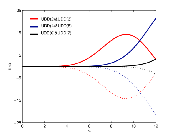
Figure 1: $t=1$. Red line: UDD(2) on the first qubit, UDD(3) on the second qubit. Solid line for $f_{2}$, and dashed line for $f_{3}$. Other four colored lines follow similar definitions.

By requiring the phase shift from Eq. ($11$) vanish, we get the equality

$$\delta_{1}-\delta_{2}+...(-1)^{n+m-1}\delta_{n+m}+\frac{(-1)^{n+m}}{2}=0.$$ (20)

This is exactly the equation to derive UDD(1). In other words, our $(n+m)$-pulse sequence has to be a first order sequence at least. Now we make the first observation: Eq. ($20$) holds for any combination of UDD($n$) and UDD($m$) with $n+m$ odd. Besides, parity plays an important role in the following relations

$$\sum_{j=1}^{m}\sum_{j^{{}^{\prime\prime}}<i^{{}^{\prime}}}^{n}(-1)^{i+j}\sin\omega{t}(\delta_{j^{{}^{\prime\prime}}}-\delta_{i^{{}^{\prime}}})$$ (21)

$$= \sum_{i=1}^{n}\sum_{i^{{}^{\prime}}>j^{{}^{\prime\prime}}}^{m}(-1)^{i+j}\sin\omega{t}(\delta_{(n+1-i)^{{}^{\prime}}}-\delta_{(m+1-j)^{{}^{\prime\prime}}}),$$

$$= \sum_{i=1}^{n}\sum_{i^{{}^{\prime}}<j^{{}^{\prime\prime}}}^{m}(-1)^{i+j+m+n}\sin\omega{t}(\delta_{i^{{}^{\prime}}}-\delta_{j^{{}^{\prime\prime}}}),$$

and

$$\sum_{j=1}^{m}(-1)^{j+n+1}\sin\omega{t}(\delta_{j^{{}^{\prime\prime}}}-1)$$ (22)

$$= -\sum_{j=1}^{m}(-1)^{j+n+1}\sin\omega{t}(\delta_{(m+1-j)^{{}^{\prime\prime}}}),$$

$$= -\sum_{j=1}^{m}(-1)^{j+n+m}\sin\omega{t}(\delta_{j^{{}^{\prime\prime}}}).$$

As a result, if $n$ and $m$ have different parity, we have

$$x_{m}(\omega{t})+z_{m}(\omega{t})+x_{n}(\omega{t})+z_{n}(\omega{t})=0.$$ (23)

Moreover, it is easy to verify

$$x_{m}(\omega{t})+z_{m}(\omega{t})-x_{n}(\omega{t})-z_{n}(\omega{t})=\Im(y_{n}(t)y_{m}^{*}(t)),$$

since

$$\sum_{i=1}^{n}\sum_{i^{{}^{\prime}}<j^{{}^{\prime\prime}}}^{m}(-1)^{i+j}\sin\omega{t}(\delta_{i^{{}^{\prime}}}-\delta_{j^{{}^{\prime\prime}}})$$ (25)

$$- \sum_{j=1}^{m}\sum_{j^{{}^{\prime\prime}}<i^{{}^{\prime}}}^{n}(-1)^{i+j}\sin\omega{t}(\delta_{j^{{}^{\prime\prime}}}-\delta_{i^{{}^{\prime}}})$$

$$= \sum_{i=1}^{n}\sum_{i^{{}^{\prime}}<j^{{}^{\prime\prime}}}^{m}(-1)^{i+j}\sin\omega{t}(\delta_{i^{{}^{\prime}}}-\delta_{j^{{}^{\prime\prime}}})$$

$$+ \sum_{j=1}^{m}\sum_{j^{{}^{\prime\prime}}<i^{{}^{\prime}}}^{n}(-1)^{i+j}\sin\omega{t}(\delta_{i^{{}^{\prime}}}-\delta_{j^{{}^{\prime\prime}}}),$$

$$= \sum_{i=1}^{n}\sum_{j=1}^{m}(-1)^{i+j}\sin\omega{t}(\delta_{i^{{}^{\prime}}}-\delta_{j^{{}^{\prime\prime}}}).$$

For $n+m$ is odd, solving Eq. ($23$) and Eq. ($24$) yields

$$f_{m}(\omega{t})=-f_{n}(\omega{t})=\Im(y_{n}(t)y_{m}^{*}(t))/2.$$ (26)

Again the phase factors $\Delta_{m}(t)$ and $\Delta_{n}(t)$ are bounded by the filter functions $y_{m}(t)$ and $y_{n}(t)$. Thus we have completed the proof that both phase and coherence can be preserved to the same order. In Fig. 1, we give three examples of independent UDD sequences with different parity, where $f_{m}(\omega{t})$ and $f_{n}(\omega{t})$ are numerically calculated. It can be seen that the phases are suppressed order by order through increasing the pulse number of each UDD sequence.

3.2 UDD Sequences with Same Parity

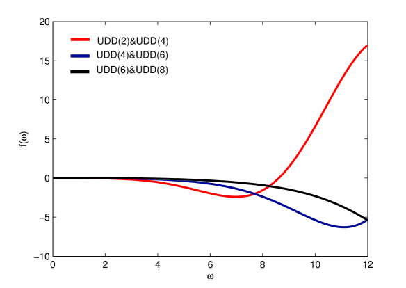
Figure 2: The same definition as Fig. 1. Note that the solid lines completely overlap the dashed counterparts as indicated by Eq. (27).

We only consider two UDD sequences of even order, and two odd-order sequences share essentially the same property because their middle pulses do not flip the collective operator $\sigma_{z_{1}}\sigma_{z_{2}}$. If $n$ and $m$ are even, from Eq. ($21$) and Eq. ($22$) we know

$$x_{n}(\omega{t})+z_{n}(\omega{t})=x_{m}(\omega{t})+z_{m}(\omega{t}).$$ (27)

A corollary is drawn: $y_{n}(t)y_{m}^{*}(t)$ is a real number if $n$ and $m$ are even. Moreover, $x_{m}(\omega{t})+z_{m}(\omega{t})$ are not bounded by filter functions anymore. As shown in Fig. 2, phase evolutions are eliminated at a fixed level. Increasing pulse number cannot improve the performance. Suppression of $f_{n}(\omega{t})$ and $f_{m}(\omega{t})$ before $\omega{t}<2$ is due to the fact: $\sin\omega{t}\approx\omega{t}$ if $\omega{t}$ is small. As a consequence, $f_{n}(\omega{t})$ and $f_{m}(\omega{t})$ are self-corrected to first order, see Eq. ($2$). While $\sigma_{z_{1}}\sigma_{z_{2}}\omega{t}$ is effectively averaged at low frequencies, the nonlinear part of $\sigma_{z_{1}}\sigma_{z_{2}}\sin\omega{t}$ is uncontrollable.

In the present model the indirect coupling via a thermal bath is commonly weak. If there exists highly nonlinear indirect coupling between the qubits, we expect more distinctions will be observed by using different UDD sequences.

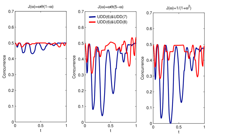
Figure 3: Evolutions of concurrence in three different environments. $\Theta(\cdot)$ is Heaviside step function. In each of the three diagrams, red line stands for the same parity, and the other colored line for different parity.

3.3 Entanglement Dynamics

In order to illustrate the difference caused by the parity, especially the distinct oscillation patterns of quantum correlation under different decoupling schemes, we numerically calculate the entanglement dynamics. The initial bipartite state is chosen to be $\frac{\sqrt{2}}{4}(|0\rangle+\sqrt{3}|1\rangle+\sqrt{3}|2\rangle+|3\rangle)$, which is partially entangled. In Fig. 3 we have used concurrence to measure the two-qubit entanglement [31].

We consider the dynamical evolution of concurrence versus time under three kinds of environmental spectrum. We can see that for $J(\omega)=\omega\Theta(1-\omega)$, the final concurrence at $t=1$ is perfectly kept at the initial level regardless of the parity. This result is consistent with our earlier observation that the low frequency part of $f(\omega{t})$ is self-corrected. However for the other two spectrums, the UDD performances are obviously dependent on the parity difference. For $J(\omega)=\omega\Theta(5-\omega)$, the combination of UDD(6) and UDD(7) still preserves the initial entanglement at the end of the decoupling cycle, while UDD(6) and UDD(8) fails to do so. Since UDD(6) and UDD(8) are not able to effectively suppress the indirect coupling between the two qubits, the quantum correlation of their final state is much larger than the initial one. Similar increase can be observed in soft-cutoff spectrum ($J(\omega)=\frac{1}{1+\omega^{2}}$). Note that in this type of spectrum concurrences cannot be well preserved in both combinations owing to severe decoherence [6, 32].

As shown in Fig. 3, concurrences undergo violent oscillations within the pulse intervals. In contrast with UDD(6) and UDD(8), the concurrence that is controlled by the combination of UDD(6) and UDD(7) drops more rapidly in the beginning. For $J(\omega)=\frac{1}{1+\omega^{2}}$, the concurrence even reach zero at one point, indicating the entanglement is completely lost. However at the final stage of the decoupling period, the sequences with different parity have a more smooth and steady concurrence, which makes them more feasible since the loose timing constraint for retrieving the final state, compared with the combination of UDD(6) and UDD(8).

4 Conclusion

In this paper we give a detailed analysis of available DD sequences which can be used to eliminate both qubit-environment and indirect qubit-qubit coupling in a common bath. Exact dynamics under arbitrary pulse sequences are derived. As we find out, it is possible to apply UDD sequences independently on each of the two qubit, and at the same time preserve the bipartite state to higher order. This result greatly simplifies the scheme of universal NUDD when dealing with correlated environments. We has proven that by applying UDD($n$) and UDD($m$) with $n+m$ odd, the evolutions of all density matrix elements are bounded by the single-qubit filter functions of UDD($n$) and UDD($m$).

In conclusion, we suggest using UDD sequences with different parity to protect a dephasing bipartite system, in case that the environments for individual qubit are not completely independent. Besides, our results may find applications in quantum information processing due to its superior ability to dynamically switch off the interaction induced by a common quantum bus.

5 Acknowledgments

Yu Pan wishes to thank Jiang-bin Gong for helpful comments on the manuscript. This work is supported by National Nature Science Foundation under Grant No. 60774099, No. 60821091, and No. 61134008.

References

References

[1] Viola L, Knill E, and Lloyd S 1999 Phys. Rev. Lett.82, 2417.
[2] Uhrig G S 2007 Phys. Rev. Lett.98, 100504.
[3] Biercuk M J 2009 et al., Nature (London)458, 996.
[4] Khodjasteh K and Lidar D A 2005 Phys. Rev. Lett.95, 180501.
[5] Khodjasteh K and Lidar D A 2007 Phys. Rev. A 75, 062310.
[6] Uhrig G S 2008 New. J. Phys.10, 083024.
[7] Mukhtar M, Saw T B, Soh W T, and Gong J B 2010 Phys. Rev. A 81, 012331.
[8] Mukhtar M, Soh W T, Saw T B, and Gong J B 2010 Phys. Rev. A 82, 052338.
[9] Agarwal G S 2010 Phys. Scr.82, 038103.
[10] Wang Z Y and Liu R B 2011 Phys. Rev. A 83, 022306.
[11] Pan Y, Xi Z, Gong J B 2011 J. Phys. B: At. Mol. Opt. Phys.44, 175501.
[12] Wang Y, Rong X, Feng P B, Xu W J, Chong B, Su J H, Gong J B, and Du J 2011 Phys. Rev. Lett.106, 040501.
[13] Roy S S, Mahesh T S, and Agarwal G S 2011 Phys. Rev. A 83, 062326.
[14] Jiang L and Imambekov A 2011 Phys. Rev. A 84, 060302(R).
[15] Quiroz G and Lidar D A 2011 Phys. Rev. A 84, 042328.
[16] Kuo W J and Lidar D A 2011 Phys. Rev. A 84, 042329.
[17] Uhrig G S and Lidar D A 2010 Phys. Rev. A 82, 012301.
[18] Khodjasteh K, Erdélyi T, and Viola L 2011 Phys. Rev. A 83, 020305(R).
[19] Kao J, Hung J, Chen P, and Mou C 2010 Phys. Rev. A 82, 062120.
[20] Xiao Z, He L, and Wang W 2011 Phys. Rev. A 83, 032322.
[21] Souza A M, Álvarez G A, and Suter D arXiv:1110.6334.
[22] Contreras-Pulido L D and Aguado R 2008 Phys. Rev. B 77, 155420.
[23] Corn B and Yu T 2009 Quantum Inf. Process.8, 565.
[24] Braun D 2002 Phys. Rev. Lett.89, 277901.
[25] Oh S and Kim J 2006 Phys. Rev. A 73, 062306.
[26] Majer J, et al. 2007 Nature (London)449, 443.
[27] Rao D D B, Bar-Gill N, and Kurizki G 2011 Phys. Rev. Lett.106, 010404.
[28] Rao D D B and Kurizki G 2011 Phys. Rev. A 83, 032105.
[29] Yuan J B, Kuang L M, and Liao J Q 2010 J. Phys. B: At. Mol. Opt. Phys.43, 165503.
[30] Weiss U 2008 Quantum Dissipative Systems (World Scientific, Singapore).
[31] Wootters W K 1998 Phys. Rev. Lett.80, 2245.
[32] Cywinski L, Lutchyn R M, Nave C P, and Das Sarma S 2008 Phys. Rev. B 77, 174509.