Chiral $\ {\mathbbm{C}}{{P}}^{2}\$skyrmions in three-band superconductors

Abstract

It is shown that under certain conditions, three-component superconductors (and in particular three-band systems) allow stable topological defects different from vortices. We demonstrate the existence of these excitations, characterized by a $\ {\mathbbm{C}}{{P}}^{2}\$topological invariant, in models for three-component superconductors with broken time reversal symmetry. We term these topological defects “chiral $GL^{(3)}$ skyrmions”, where “chiral” refers to the fact that due to broken time reversal symmetry, these defects come in inequivalent left- and right-handed versions. In certain cases these objects are energetically cheaper than vortices and should be induced by an applied magnetic field. In other situations these skyrmions are metastable states, which can be produced by a quench. Observation of these defects can signal broken time reversal symmetry in three-band superconductors or in Josephson-coupled bilayers of $s_{\pm}$ and $s$-wave superconductors.

I Introduction

Experiments on the recently discovered iron pnictide superconductors suggest the existence of positive coefficient of Josephson coupling between superconducting components in two bands ($s_{\pm}$ state) and possibly more than two superconducting bands iron2 . Under these circumstances, new physics can appear. That is, frustration of competing interband Josephson couplings in three-component superconductors, can lead to spontaneously Broken Time Reversal Symmetry (BTRS) nagaosa ; stanev (another scenario for BTRS states in pnictides was discussed in Refs. zhang, ; honerkamp, ). There, the ground state explicitly breaks the discrete $\mbox{U(1)}\times{\mathbbm{Z}}_{2}$ symmetry Garaud.Carlstrom.ea:11 ; Carlstrom.Garaud.ea:11a . Related multicomponent states were also recently discussed, in connection with other materials agterberg2011 . If superconductivity in iron pnictides is described by just a two-band $s_{\pm}$ models, BTRS states can nonetheless be obtained in a Josephson-coupled bilayer of $s_{\pm}$ superconductor and ordinary $s$-wave material nagaosa . Such bilayer systems can be effectively described by a three-component model where the third component is coupled through a “real-space” inter-layered Josephson coupling.

Due to a number of unconventional phenomena, which are not possible in two-band superconductors, the possible experimental realization of three component superconductors (either with or without BTRS) recently started to attract substantial interest stanev ; hu ; Garaud.Carlstrom.ea:11 ; Carlstrom.Garaud.ea:11a ; stanev2 ; machida3 ; levchenko ; nitta ; Lin:12 . These phenomena include: exotic collective modes which are different from the Leggett’s mode massless ; Carlstrom.Garaud.ea:11a ; stanev2 ; the existence of a large disparity in coherence lengths even when intercomponent Josephson coupling is very strong, leading to type-1.5 regimes Carlstrom.Garaud.ea:11a (where some coherence lengths are smaller and some are larger than the magnetic field penetration length bs1 ); the possibility of flux-carrying topological solitons different from Abrikosov vortices Garaud.Carlstrom.ea:11 .

This paper is a follow-up to Ref. Garaud.Carlstrom.ea:11, where we introduced new flux-carrying topological solitons. Here we study in detail, these topological solitons which we term chiral $GL^{(3)}$ skyrmions (chiral skyrmions for short). They are magnetic flux-carrying excitations characterized by a $\ {\mathbbm{C}}{{P}}^{2}\$topological invariant, (by contrast this invariant is trivial for ordinary vortices). The topological properties, motivating the denomination skyrmion are rigorously discussed. As the terminology suggests, the soliton itself has a given chiral state of the Broken Time Reversal Symmetry. More precisely, different arrangements of the fractional vortices constituting a skyrmion carrying integer flux define different chirality of the skyrmion. Finally $GL^{(3)}$ refers to the physical context of the three-component Ginzburg–Landau theory. The thermodynamic and energetic (meta)stability of chiral skyrmions are discussed, as well as their perturbative stability. In scanning SQUID, scanning Hall or magnetic force microscopy experiments, chiral $GL^{(3)}$ skyrmions can (under certain conditions) be distinguished from vortices by their very exotic magnetic field profile. Fig. 1 shows examples of such exotic magnetic field signatures of chiral skyrmions in three band superconductors with various parameters of the model.

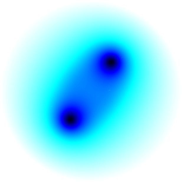
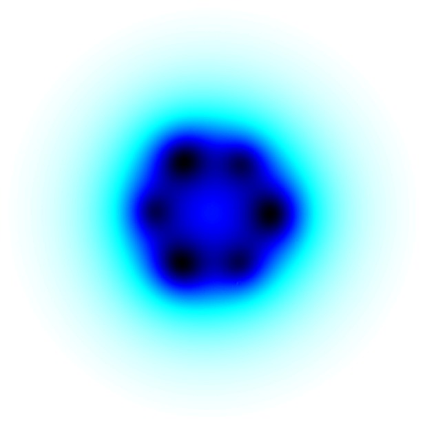
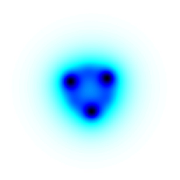
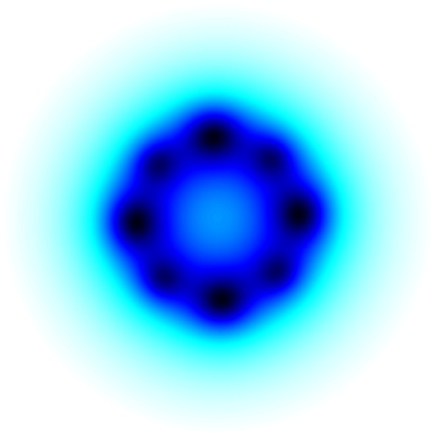
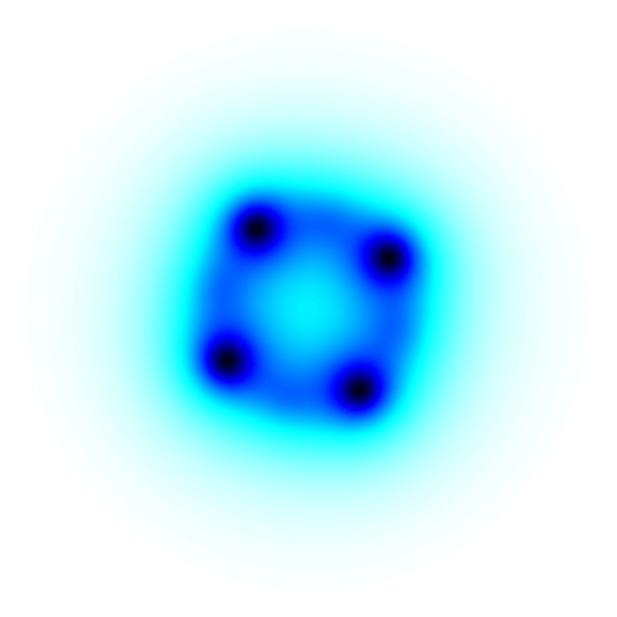
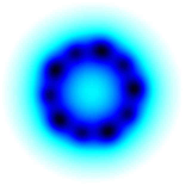
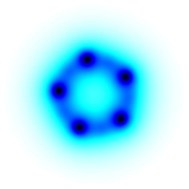
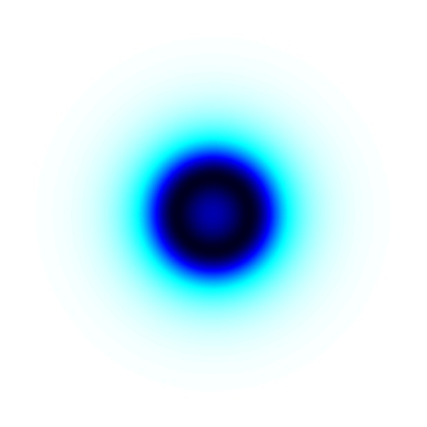
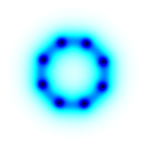
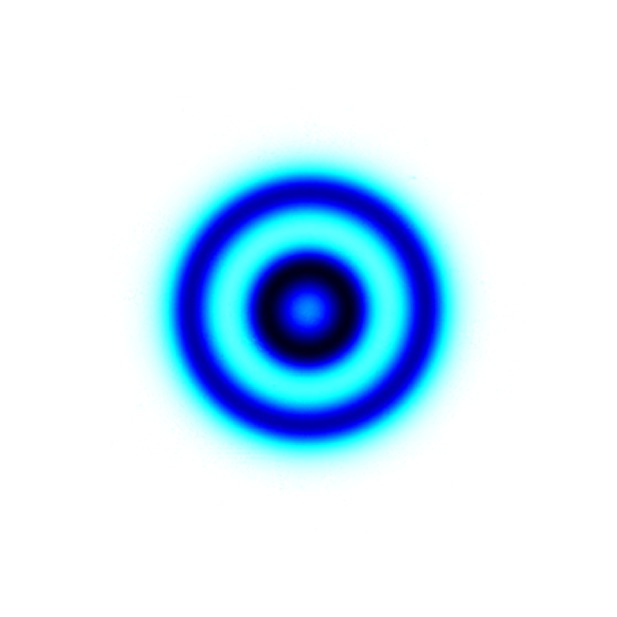
Figure 1: (Color online) – Example of unusual observable magnetic field configuration of chiral skyrmions.

The paper is organized as follows. In Sec. II we introduce a Ginzburg-Landau model for three-component superconductors where phase frustration due to competing Josephson interactions leads to Broken Time Reversal Symmetry states. The structure of the domain walls which are possible due to this new spontaneously broken ${\mathbbm{Z}}_{2}$ symmetry is discussed in Sec. II.1. The essential concepts of the topological excitations in multi-band superconductors are discussed in Sec. II.3. After that, the new kind of topological excitations, chiral $GL^{(3)}$ skyrmions, are discussed Sec. II.4. The physical properties: (i) energy of formation of a skyrmion versus vortex lattice, (ii) thermodynamical stability of the chiral skyrmions and (iii) their perturbative stability are investigated Sec. III. In the next part, Sec. IV, the very rich interactions between the chiral skyrmions and between skyrmions and vortices are investigated. The model has many interesting mathematical aspects as well. Sec. V is devoted to the most formal aspects and rigorous justifications of the physics and mathematical properties of the three-component Ginzburg–Landau model and the skyrmionic excitations therein. This section aims at a more mathematical audience. Thus, readers less interested in formal justification of the physics can skip these discussions, and go straight after Sec. IV to our conclusions in Sec. VI. There we conclude this paper by addressing, in more detail, the possible experimental signatures of our chiral $GL^{(3)}$ skyrmions.

II The model

In this paper we consider various realizations of three-component superconductivity described by the following three-component Ginzburg–Landau (GL) model:

$$\mathcal{F} =\frac{1}{2}(\nabla\times\boldsymbol{A})^{2}+\sum_{a}\frac{1}{2}|\boldsymbol{D}\psi_{a}|^{2}+\alpha_{a}|\psi_{a}|^{2}+\frac{1}{2}\beta_{a}|\psi_{a}|^{4}$$

$$+ \sum_{a,b>a}\gamma_{ab}|\psi_{a}|^{2}|\psi_{b}|^{2}-\eta_{ab}|\psi_{a}||\psi_{b}|\cos(\varphi_{b}-\varphi_{a})\,.$$ (2.1)

Here $\boldsymbol{D}=\nabla+ie{\boldsymbol{A}}$ and $\psi_{a}=|\psi_{a}|e^{i\varphi_{a}}$ are complex fields representing the superconducting components. The component indices $a,b$ take the values $1,2,3$. In the particular case of a three-band superconductor, different superconducting components arise due to Cooper pairing in three different bands. The bands are coupled by their interaction with the vector potential $\boldsymbol{A}$ and also through potential interactions. The coefficients $\eta_{ab}$ are the intercomponent Josephson couplings. We also consider the more general case which includes bi-quadratic density interactions with the couplings $\gamma_{ab}$. Here, the London magnetic field penetration length is parametrized by the gauge coupling constant $e$. Functional variation of the free energy (II) with respect to the fields gives Ginzburg-Landau equations

$$\boldsymbol{D}\boldsymbol{D}\psi_{a}=2\frac{\partial V}{\partial\psi_{a}^{*}}\,,\leavevmode\nobreak\ \leavevmode\nobreak\ \leavevmode\nobreak\ \leavevmode\nobreak\ \partial_{i}\left(\partial_{i}A_{j}-\partial_{j}A_{i}\right)=J_{i}\,.$$ (2.2)

where $V$ is the collection of all non-gradient terms and the supercurrent is defined as

$$\boldsymbol{J}\equiv\sum_{a=1,2,3}\boldsymbol{J}^{(a)}=\sum_{a=1,2,3}e\mathrm{Im}\left(\psi_{a}^{*}\boldsymbol{D}\psi_{a}\right)\,.$$ (2.3)

In multiband superconductors, a Ginzburg–Landau expansion of this kind can in certain cases be formally justified microscopically (see e.g. corresponding discussion in two-band case silaev ). In what follows, different physical realizations of the model (II) with different broken symmetries are considered. Note that in some of the physical realizations of multicomponent GL models, some of the couplings are forbidden (for example on symmetry grounds). This can occur for intercomponent Josephson couplings, in some realizations frac ; *smiseth. More terms, consistent with symmetries, can be included to extend the GL functional. Alternatively a microscopic approach can provide a more quantitatively accurate picture at lower temperatures. However, the properties of the topological objects which are discussed, should then differ only quantitatively and not qualitatively in the framework of e.g. microscopic approach for a system with a given symmetry (some examples how phenomenological multiband GL models give good results even at low temperature can be found in Ref. silaev, ).

The field configurations considered in the following are two-dimensional, as well as three dimensional systems with translation invariance along the third axis.

II.1 Broken Time Reversal Symmetry, the $U(1)\times{\mathbbm{Z}}_{2}$ states

For a given parameter set $(\alpha_{a},\beta_{a},\eta_{ab},\gamma_{ab})$, the ground state is the field configuration which minimizes the potential energy. The corresponding values of $|\psi_{a}|$’s and $\varphi_{a}$’s, together with the gauge coupling $e$ determine the physical length scales of the theory. The particularly interesting property of the model (II), is that the ground state can be qualitatively different from its two band counterparts. While in two bands systems with Josephson interactions the phase-locking is trivial (either $0$ or $\pi$), the phase-locking in three bands can be much more involved. Indeed, competition between different phase-locking terms possibly leads to phase frustration. When $\eta_{ab}>0$, the corresponding Josephson term is minimal for zero phase difference, while if $\eta_{ab}<0$ it is minimal for $\varphi_{ab}\equiv\varphi_{b}-\varphi_{a}=\pi$. Now if the signs of $\eta_{ab}$’s are all positive (we denote it as $[+++]$), the ground state has $\varphi_{1}=\varphi_{2}=\varphi_{3}$. Similarly for $[+--]$ couplings, the phase locking pattern $\varphi_{1}=\varphi_{2}=\varphi_{3}+\pi$. However for $[++-]$ or $[---]$, the phase locking terms are frustrated. That is: all three Josephson terms cannot simultaneously attain their minimal values. As a result ground state phase differences are neither $0$ nor $\pi$. For example, consider the case $\alpha_{a}=-1,\;\beta_{a}=1$ and $\eta_{ab}=-1$. Symmetry under global U(1) phase rotations allows to set $\varphi_{1}=0$ without loss of generality (for the below considerations). There, two ground states are possible $\varphi_{2}=2\pi/3,\;\varphi_{3}=-2\pi/3$ or $\varphi_{2}=-2\pi/3,\;\varphi_{3}=2\pi/3$. The two ground states are each other’s complex conjugate. The actual values of the ground state phases depend on the potential parameters.

Note that the free energy is invariant under complex conjugation, $(\psi_{1},\psi_{2},\psi_{3})\mapsto(\psi_{1}^{*},\psi_{2}^{*},\psi_{3}^{*})$, which takes it to a state with different phase locking. Thus the theory has a spontaneously broken discrete (${\mathbbm{Z}}_{2}$) symmetry, called Time Reversal Symmetry. That is, the free energy is still invariant under complex conjugation, but the ground state is not. By ‘picking’ one of the two inequivalent phase-locking patterns, the ground state explicitly breaks the discrete ${\mathbbm{Z}}_{2}$ symmetry. Such states are termed Broken Time Reversal Symmetry (BTRS) states.

II.2 Domain walls in BTRS states

                 

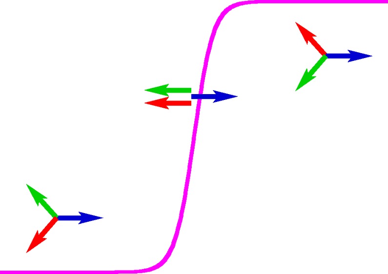
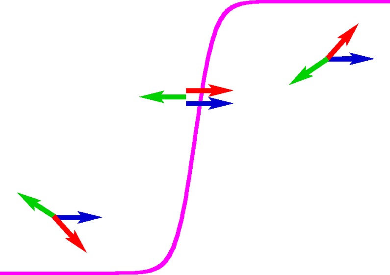
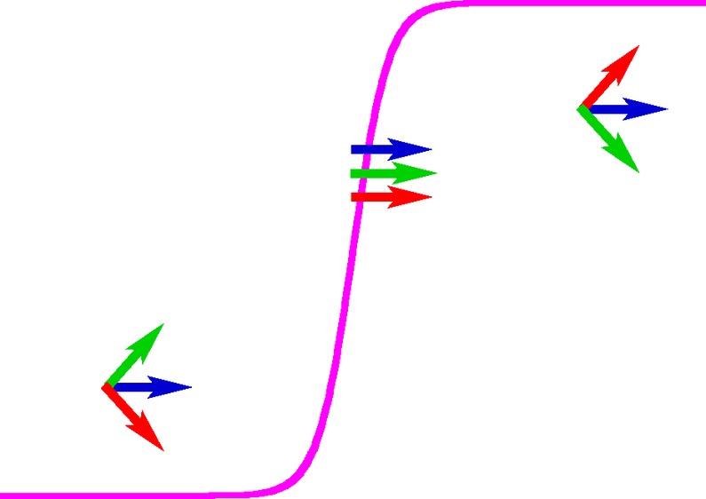
Figure 2: (Color online) – Representation of the vacuum submanifold (Top), for $(\alpha_{a},\beta_{a})=(-1,1)$ and $\eta_{ab}=-3$. The image shows the potential energy as a function of the phase differences: $\varphi_{2}$ and $\varphi_{3}$, minimized with respect to all moduli degrees of freedom (while $\varphi_{1}$ is set to zero by U(1) invariance associated with simultaneous change of all phases). Red and green dots show inequivalent ${\mathbbm{Z}}_{2}$ ground states. And the lines connecting them represent four different kinds of domain wall trajectory over the field manifold. Black dots are ground states located farther than $2\pi$ in the phase differences. The second line, gives a schematic representation of various ${\mathbbm{Z}}_{2}$ domain walls in three-band superconductors with different frustrations of phase angles, shown by arrows of different colors. The pink line schematically shows the phase difference between red and green arrow, interpolating between the two inequivalent ground states.

BTRS systems have topological excitations related to the broken discrete symmetry in the form of domain walls. The domain walls interpolate between domains of inequivalent ground states. In other words they are walls separating regions of different phase locking. It is instructive to display more quantitatively the structure of the ground state (or “vacuum”) manifold, see Fig. 2. There, the potential energy is minimized with respect to the densities $|\psi_{a}|$, for uniform fixed phase difference configurations. This provides a map of the ground state manifold. It appears clearly that there are disconnected inequivalent ground states (the red and green dots). Interestingly, there is not a unique path to connect inequivalent ground states with inequivalent phase locking, but four. The four corresponding domain walls will have different line tension (energy per unit length). Note that, investigating the vacuum manifold with fixed ground state densities $|\psi_{a}|$ (at their true ground state value) provides a qualitatively similar picture. Namely, this approximation preserves the positions of the minima. However, the actual values of $\mathcal{F}_{\mbox{\tiny pot}}$ are obviously different if $|\psi_{a}|$’s are held constant to the ground state, so this approximation does not allow one to calculate the energy of the domain walls. In particular the sharp angles appear there for strong Josephson couplings, when the ground state densities are not fixed. This property is absent when densities are held to their actual ground state values.

II.3 Flux-carrying topological defects in three component Ginzburg–Landau model

As previously stated, three component Ginzburg–Landau model can exhibit BTRS and domain wall excitations associated with the broken ${\mathbbm{Z}}_{2}$ symmetry. There are also different topological defects, associated with the other broken symmetries.

Our main interest, here, is three-component skyrmionic solutions of the Ginzburg–Landau model. Here skyrmions are topological defects characterized by a topological invariant which classifies the maps ${\mathbb{R}}^{2}\to{\mathbb{C}}{{P}}^{2}$. In contrast to the topological invariant characterizing vortices (i.e. the winding number which is defined as a line integral over a closed path), the topological index associated with skyrmionic excitations is given as an integral over $xy$-plane :

$$\mathcal{Q}(\Psi)=\int_{\mathbbm{R}^{2}}\frac{i\epsilon_{ji}}{2\pi|\Psi|^{4}}\left[|\Psi|^{2}\partial_{i}\Psi^{\dagger}\partial_{j}\Psi+\Psi^{\dagger}\partial_{i}\Psi\partial_{j}\Psi^{\dagger}\Psi\right]\text{d}^{2}x\,,$$ (2.4)

with $\Psi^{\dagger}=(\psi_{1}^{*},\psi_{2}^{*},\psi_{3}^{*})$. A detailed derivation of this formula is given in Sec. V. If we have an axially symmetry vortex with a core where all superconducting condensates simultaneously vanish, then $\mathcal{Q}=0$. On the other hand, if singularities happen at different locations, then $\mathcal{Q}\neq 0$ and the quantization condition $\mathcal{Q}=\boldsymbol{B}/\Phi_{0}=N$ holds ( $\Phi_{0}$ being the flux quantum and $N$ the number of flux quanta). This is rigorously discussed in Sec. V.2.

Fractional vortices

In order to understand the physical properties of the later introduced chiral skyrmions, it is good to remind oneself of the basic features of multi-component superconductors and their topological excitations. The elementary vortex excitations in this system are fractional vortices. They are defined as field configurations with a $2\pi$ phase winding only in one phase (e.g. $\varphi_{1}$ has $\Delta\varphi_{1}\equiv\oint\nabla\varphi_{1}=2\pi$ winding while $\Delta\varphi_{2}=\Delta\varphi_{3}=0$). To better illustrate their physical properties, the Ginzburg–Landau free energy (II) can be rewritten as

$$\mathcal{F} =\frac{1}{2}(\nabla\times\boldsymbol{A})^{2}+\frac{\boldsymbol{J}^{2}}{2e^{2}\rho^{2}}$$ (2.5a)

$$+\sum_{a}\frac{1}{2}(\nabla|\psi_{a}|)^{2}+\alpha_{a}|\psi_{a}|^{2}+\frac{\beta_{a}}{2}|\psi_{a}|^{4}$$ (2.5b)

$$+\sum_{a,b>a}\frac{|\psi_{a}|^{2}|\psi_{b}|^{2}}{\rho^{2}}\left(\frac{(\nabla\varphi_{ab})^{2}}{2}-\frac{\eta_{ab}\rho^{2}\cos\varphi_{ab}}{|\psi_{a}||\psi_{b}|}\right)$$ (2.5c)

$$+\sum_{a,b>a}\gamma_{ab}|\psi_{a}|^{2}|\psi_{b}|^{2}\,,$$ (2.5d)

where $\varphi_{ab}\equiv\varphi_{b}-\varphi_{a}$ are the phase differences and $\rho^{2}=\sum_{a}|\psi_{a}|^{2}$. The indices $a,b$ again denote the different superconducting condensates and take value $1,2,3$. The identity

$$\sum_{a=1}^{n}\sum_{b=1}^{n}|\psi_{a}|^{2}|\psi_{b}|^{2}\nabla\varphi_{a}\left(\nabla\varphi_{a}-\nabla\varphi_{b}\right)$$

$$=\sum_{a=1}^{n}\sum_{b=a+1}^{n}|\psi_{a}|^{2}|\psi_{b}|^{2}\left(\nabla\varphi_{a}-\nabla\varphi_{b}\right)^{2}\,,$$ (2.6)

is used to derive this expression. Here, the supercurrent (2.3) reads, more explicitly

$$\boldsymbol{J}/e=e\rho^{2}\boldsymbol{A}+\sum_{a}|\psi_{a}|^{2}\nabla\varphi_{a}\,.$$ (2.7)

Consider now a vortex for which the phase of only one component changes by $2\pi$: $\oint\nabla\varphi_{a}=2\pi$. Such a configuration carries a fraction of flux quantum frac ; *smiseth

$$\Phi_{a}=\oint_{\sigma}\boldsymbol{A}\text{d}\boldsymbol{\ell}=\frac{|\psi_{a}|^{2}}{\rho^{2}}\frac{1}{e}\oint_{\sigma}\nabla\varphi_{a}=\frac{|\psi_{a}|^{2}}{\rho^{2}}\Phi_{0}\,,$$ (2.8)

where $|\psi_{a}|$ denotes the ground state density of $\psi_{a}$, $\sigma$ is a closed curve around the vortex core, and $\Phi_{0}=2\pi/e$ is the flux quantum. For vanishing Josephson interactions, the symmetry is $[U(1)]^{3}$ and each fractional vortex has logarithmically diverging energy frac ; *smiseth. This can be seen easily in the London limit by setting $\psi_{a}=\mathrm{const}$ everywhere except a sharp cutoff in the vortex core. There the terms (2.5d) and (2.5b) give trivial contribution to the free energy, so that the relevant parts now reads

$$\mathcal{F}_{\mbox{\tiny London}}=\frac{1}{2}(\nabla\times\boldsymbol{A})^{2}+\frac{\boldsymbol{J}^{2}}{2e^{2}\rho^{2}}$$

$$+\sum_{a,b>a}\frac{|\psi_{a}|^{2}|\psi_{b}|^{2}}{2\rho^{2}}\left((\nabla\varphi_{ab})^{2}-\frac{2\eta_{ab}\rho^{2}}{|\psi_{a}||\psi_{b}|}\cos\varphi_{ab}\right).$$ (2.9)

In a $[U(1)]^{3}$ symmetric model, one fractional vortex gives logarithmically divergent contribution to the energy through the term

$$\int_{r_{c}}^{r}r^{\prime}\text{d}r^{\prime}\int_{0}^{2\pi}\text{d}\theta\frac{|\psi_{a}|^{2}|\psi_{b}|^{2}}{2\rho^{2}}(\nabla\varphi_{ab})^{2}=\pi\frac{|\psi_{a}|^{2}|\psi_{b}|^{2}}{\rho^{2}}\ln{\frac{r}{r_{c}}}\,,$$ (2.10)

$r_{c}$ being a sharp cut-off corresponding to the core size of a vortex. However a bound state of three such vortices (where each phase $a=1,2,3$ had $2\pi$ phase winding) has finite energy. Indeed such a bound state has no winding in the phase differences. This finite-energy bound state is a “composite” vortex having one core singularity where $|\psi_{1}|+|\psi_{2}|+|\psi_{3}|=0$. Around this core all three phases have similar winding $\Delta\varphi_{a}=2\pi$. A vortex carrying one quantum $\Phi_{0}$ of flux is thus a logarithmically bound state of fractional vortices. For non-zero Josephson coupling, fractional vortices interact linearly, so they are bound much more strongly frac ; *smiseth. It can be seen that, for non-zero Josephson coupling, the phase difference sector (2.5c) or the second line in (II.3) is a sine-Gordon model. There, a given fractional vortex excites two Josephson strings (one per phase difference sector). Crossections of a string, at a large distance from a vortex are sine-Gordon kinks. Such a Josephson string, has an energy proportional to its length. Thus for non-zero Josephson coupling one fractional vortex has linearly diverging energy (see App. A for a detailed derivation). Note that the Josephson strings are different topological excitations than the domain walls previously discussed. Having linearly diverging energy, fractional vortices interact linearly. As a result an (composite) integer flux vortex can be seen as a strongly bound state of three co-centered fractional vortices. This binding is thus much stronger for non-zero Josephson couplings. Because of their diverging energies, the fractional vortices are not thermodynamically stable in bulk samples frac ; *smiseth: A group of three different fractional vortices is energetically unstable with respect to collapse into an integer flux composite vortex. Note however that under certain conditions, in a finite sample, they can be thermodynamically stable near boundaries silaev2 with strings terminating on a boundary.

Note that in a London limit, magnetic field of fractional vortices is exponentially localized. However in a $[U(1)]^{3}$ Ginzburg-Landau model, the magnetic field of a fractional vortices is in a general localized only according to a power law and moreover can invert direction juha .

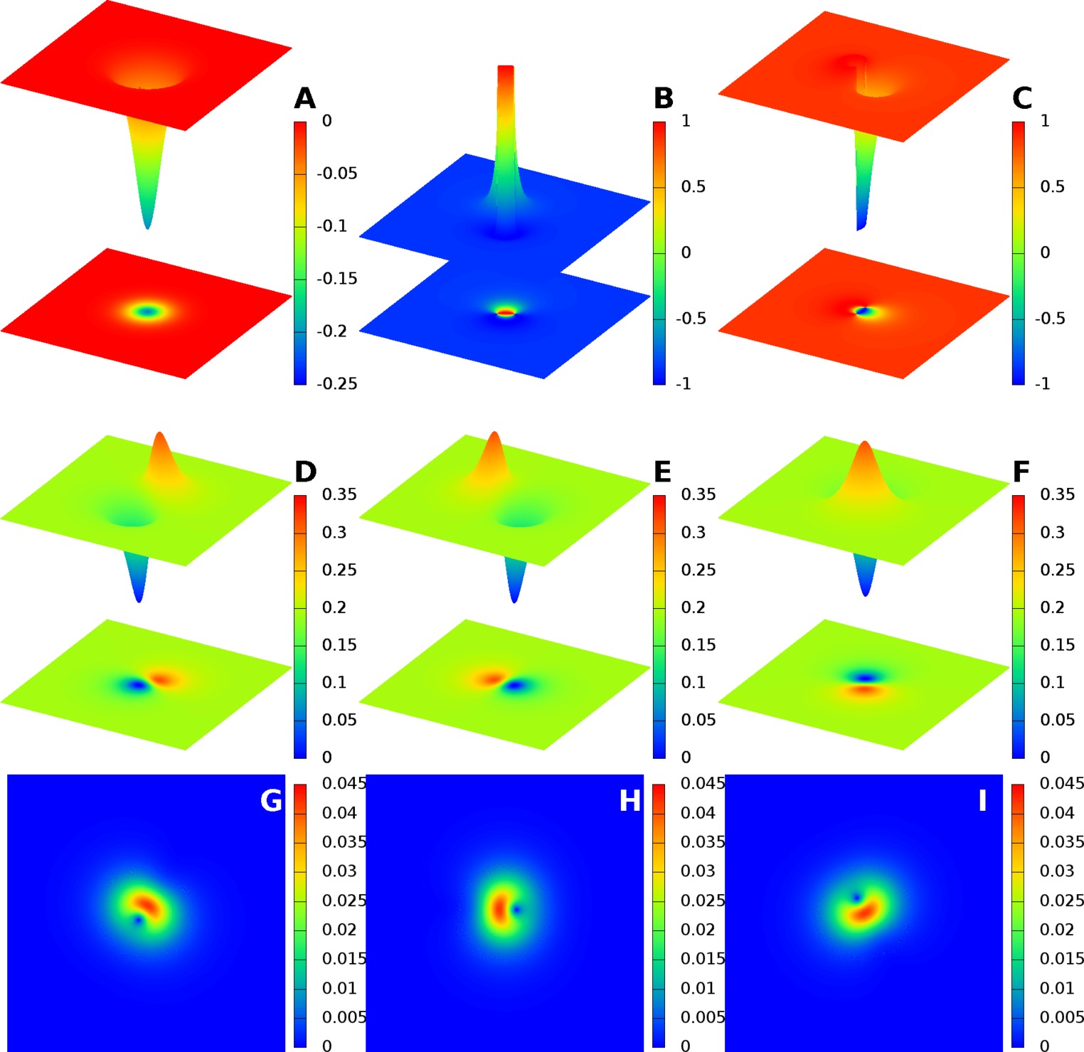
Figure 3: (Color online) – A single charge chiral skyrmion, for 3 mirror passive bands $(\alpha_{a},\beta_{a})=(1,1)$ and Josephson coupling constants $\eta_{ab}=-3$. Here $\gamma_{ab}=0.8$ and the gauge coupling constant is $e=0.6$. Displayed quantities are the magnetic flux $(\bf{A})$ and the sine of phase differences $\sin(\varphi_{12})$ $(\bf{B})$, $\sin(\varphi_{13})$ $(\bf{C})$. Condensate densities $|\psi^{2}_{1}|$, $(\bf{D})$, $|\psi^{2}_{2}|$, $(\bf{E})$ and $|\psi^{2}_{3}|$, $(\bf{F})$ are represented on the second line. The corresponding supercurrent densities $|J_{1}|$, $(\bf{G})$, $|J_{2}|$, $(\bf{H})$ and $|J_{3}|$, $(\bf{I})$ are displayed on the third line. To avoid redundant informations, the total energy density is not displayed. It qualitatively follows the magnetic flux shown in panel $(\bf{A})$.

II.4 Chiral three component Ginzburg–Landau skyrmions

Domain-walls such as those discussed in Sec. II.1 can form dynamically in physical systems by a quench. Because of its line tension, a closed domain wall collapses to zero size. From the term (2.5c), in the rewritten Ginzburg–Landau functional, it is clear that in order to decrease the energy cost associated with a gradient in the relative phase $\varphi_{ab}$, the densities of the components $|\psi_{a}|$, $|\psi_{b}|$ should be suppressed on the domain wall. Furthermore, on a domain wall, the cosines of phase differences $\cos(\varphi_{b}-\varphi_{a})$ are energetically unfavorable. Indeed, by definition, it is where they are the farthest from their ground state values. As a result, if an integer composite vortex is placed on the domain wall, the Josephson terms should tend to split it into fractional flux vortices, allowing it to attain more favorable phase difference values in between the split fractional vortices. As a consequence of these circumstances, the domain wall can trap vortices. Recall that away from domain walls, fractional vortices are linearly confined by Josephson terms.

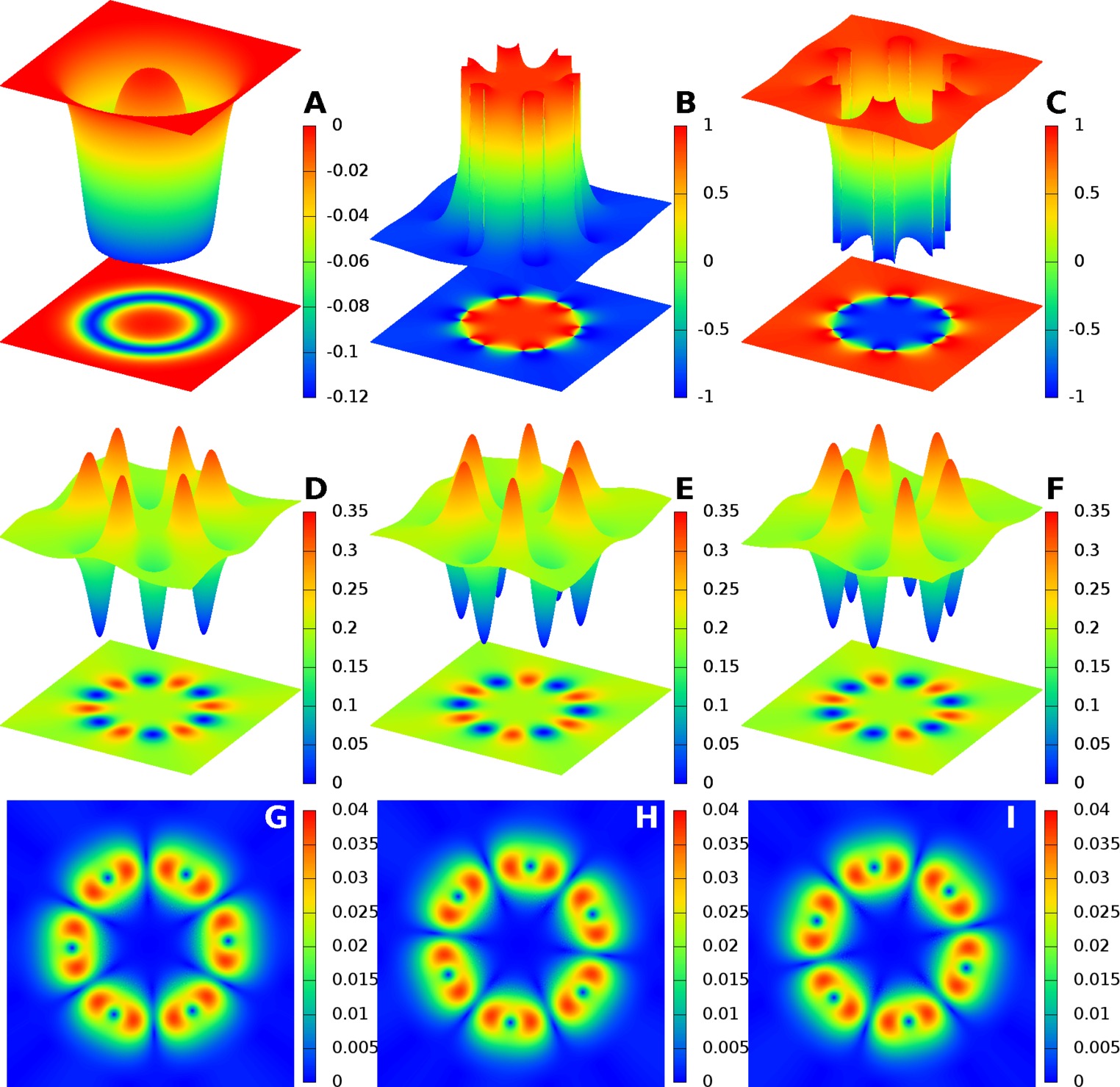
Figure 4: (Color online) – A Skyrmion with $\mathcal{Q}=6$ topological charge (which implies that it carries six flux quanta and consists of 18 fractional vortices). Displayed quantities are the magnetic flux $(\bf{A})$ and the sine of phase differences $\sin(\varphi_{12})$ $(\bf{B})$ $\sin(\varphi_{13})$ $(\bf{C})$. Condensate densities $|\psi^{2}_{1}|$, $(\bf{D})$, $|\psi^{2}_{2}|$, $(\bf{E})$ and $|\psi^{2}_{3}|$, $(\bf{F})$ are represented on the second line. The corresponding supercurrent densities $|J_{1}|$, $(\bf{G})$, $|J_{2}|$, $(\bf{H})$ and $|J_{3}|$, $(\bf{I})$ are displayed on the third line. Parameters are the same as in Fig. 3.

When the magnetic field penetration length is sufficiently large ($e$ small enough), the repulsion between the fractional vortices confined on the domain wall can become strong enough to overcome the domain wall’s tension. It thus results in a formation of a topological soliton made up of $3N$ fractional vortices, stabilized by competing forces. Such ‘composite’ topological solitons are thus made of a closed domain wall along which there are $N$ singularities in each condensate $|\psi_{a}|$. Around each singularity the phase $\varphi_{a}$ changes by $2\pi$. The total phase winding around the soliton is then $\oint\nabla\varphi_{1}\text{d}\boldsymbol{\ell}=\oint\nabla\varphi_{2}\text{d}\boldsymbol{\ell}=\oint\nabla\varphi_{3}\text{d}\boldsymbol{\ell}=2\pi N$. Therefore it carries $N$ flux quanta. The $\ {\mathbbm{C}}{{P}}^{2}\$topological invariant (2.4) computed for such objects is found to be integer, whereas it is zero for ordinary composite vortices. As a result, the composite configuration made out of a domain wall between two ${\mathbbm{Z}}_{2}$ domains stabilized by repulsion between trapped vortices, is in fact a distinct topological defect: Chiral $GL^{(3)}$ skyrmion (chiral skyrmion for short).

It was previously demonstrated that these topological defects exist and are indeed at least metastable Garaud.Carlstrom.ea:11 . Here we further investigate these objects. To investigate the existence and stability of the so-called chiral skyrmions, we use an energy minimization approach, using non-linear conjugate gradient algorithm. More details about the employed numerical schemes are provided in App. B. The topological charge (2.4) was computed numerically for all configurations and was found to be integer within small numerical errors, less than $0.1\%$, thus providing an estimate of the accuracy of our solutions.

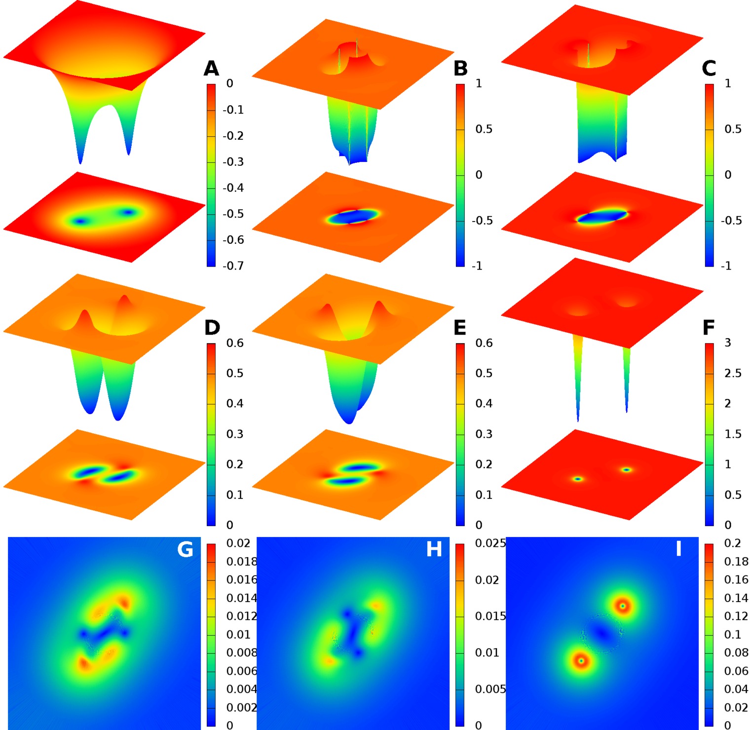
Figure 5: (Color online) – A $\mathcal{Q}=2$ quantum soliton in a system with two identical passive bands $(\alpha_{a},\beta_{a})=(1,1)$ ($a=1,2$) coupled to a third active band with substantial disparity in the ground state densities $(\alpha_{3},\beta_{3})=(-2.75,1)$. Josephson coupling constants are $\eta_{12}=\eta_{13}=\eta_{23}=-3$. The system is in a strongly type-II regime $e=0.08$, the solutions here are stable even in the absence of bi-quadratic density interaction i.e. $\gamma_{ab}=0$. Displayed quantities are the magnetic flux $(\bf{A})$ and the sine of phase differences $\sin(\varphi_{12})$ $(\bf{B})$ $\sin(\varphi_{13})$ $(\bf{C})$. Condensate densities $|\psi^{2}_{1}|$, $(\bf{D})$, $|\psi^{2}_{2}|$, $(\bf{E})$ and $|\psi^{2}_{3}|$, $(\bf{F})$ are represented on the second line. The corresponding supercurrent densities $|J_{1}|$, $(\bf{G})$, $|J_{2}|$, $(\bf{H})$ and $|J_{3}|$, $(\bf{I})$ are displayed on the third line.

Fig. 3 shows a $\mathcal{Q}=1$ chiral skyrmion in a superconductor with three passive bands (i.e. the quadratic terms have positive prefactors $\alpha_{a}$). The fact that the bands are passive is not important for the soliton’s existence. It consists of three fractional vortices, each one carrying a fraction $|\psi_{a}|^{2}/\rho^{2}$ of magnetic flux which adds up to a flux quantum $\Phi_{0}$. Since the fractional vortices are located quite close to each other they cannot be distinguished in the magnetic field profile in this case. Single charge skyrmions are more difficult to obtain than higher-charge skyrmions in this model. As will be explained later, increasing the number of flux quanta $N$, usually makes the solution more stable (which contrasts with vortices where, in the type-II regime only $N=1$ vortices are stable). The bi-quadratic density interactions in the model (II) help to stabilize $\mathcal{Q}=1$ solutions. Single charge solitons are thus usually supported by bi-quadratic density interactions. Clearly, from the density plots (panels $(\bf{D}$–$\bf{F})$) in Fig. 3, each component has a non-overlapping zero (the blue spots). A feature which can be observed in this regime is the strong density overshoot opposite to the cores (the red spots).

Higher charge skyrmions are easily formed in many cases even when there is no bi-quadratic density interaction. There, the stability of the skyrmion against collapse of the domain wall is supported only by the electromagnetic repulsion and Josephson interactions. In different numerical simulations we quite easily constructed thousands of different skyrmionic configurations, for very different parameter sets. A sample of the various skyrmions is given in the Figures 3–7. More regimes are given in the appendix App. C. For all such configurations the $\ {\mathbbm{C}}{{P}}^{2}\$topological charge (2.4) is integer with very good accuracy ( $|\mathcal{Q}/N-1|<10^{-3}$ ).

One key feature, in the Figures 3–7, is seen in the phase differences on panels $(\bf{B})$ and $(\bf{C})$. In each of these various regimes, the phase locking pattern ‘inside’ the skyrmion is different from ‘outside’, thus corresponding to either of the two ${\mathbbm{Z}}_{2}$ inequivalent ground states. As a result the chiral skyrmions (in contrast to non-chiral) feature a domain wall separating the regions of different BTRS states. As discussed below Sec. IV.2, the choice of one of the ${\mathbbm{Z}}_{2}$ ground states inside the skyrmion dictates a clockwise versus counter-clockwise arrangement of fractional vortices, thus motivating the terminology “chiral” for these topological defects.

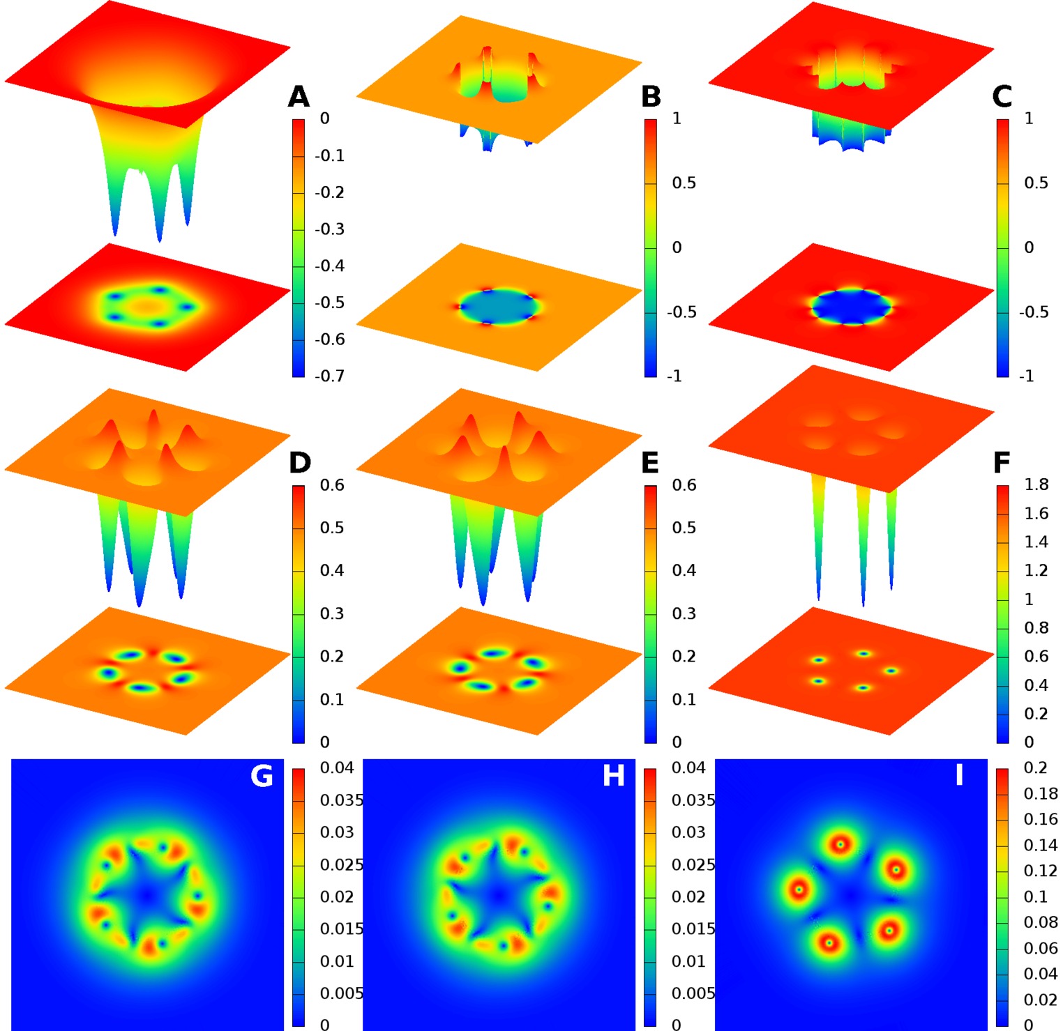
Figure 6: (Color online) – A $\mathcal{Q}=5$ quantum soliton in a system with two identical passive bands as in Fig. 5 coupled to a third active band with disparity in the ground state densities $(\alpha_{3},\beta_{3})=(-1.5,1)$. Josephson coupling constants are $\eta_{23}=-3$ and $\eta_{12}=\eta_{13}=1$. Here $e=0.2$ and there is no density-density interaction term $\gamma_{ab}=0$. The system is shaped as a pentagon deformed by the vortices of the strong active band carrying larger fractions of flux quantum. Displayed quantities are the same as in the previous pictures, e.g. Fig. 5.

Chiral skyrmions exhibit very unusual signatures of the magnetic field which can be seen from the panel $(\bf{A})$ in all of the Figures 3–7 or in Fig. 1. If the bands have similar density, each fractional vortex carries a similar fraction of flux quantum. As a result, the magnetic flux is almost uniformly spread along the domain wall, as in Fig. 4. On the other hand, when the condensates have quite different densities, the magnetic flux is carried non-uniformly by fractional vortices in different condensates. Consequently, the magnetic flux is inhomogeneously distributed along the soliton. This can be seen in Fig. 5 where the third component carries a great fraction of the flux. The remaining fraction of flux is spread along the components having less density. The overall configuration can easily be mistaken for a vortex pair in such a superconductor. For higher topological charge, the same system exhibits geometric structures (a pentagon as in Fig. 6) where the vertices are occupied by the fractional vortices of the band with bigger density. There again, geometrical arrangement of apparent vortices is a very typical signature of the chiral skyrmions.

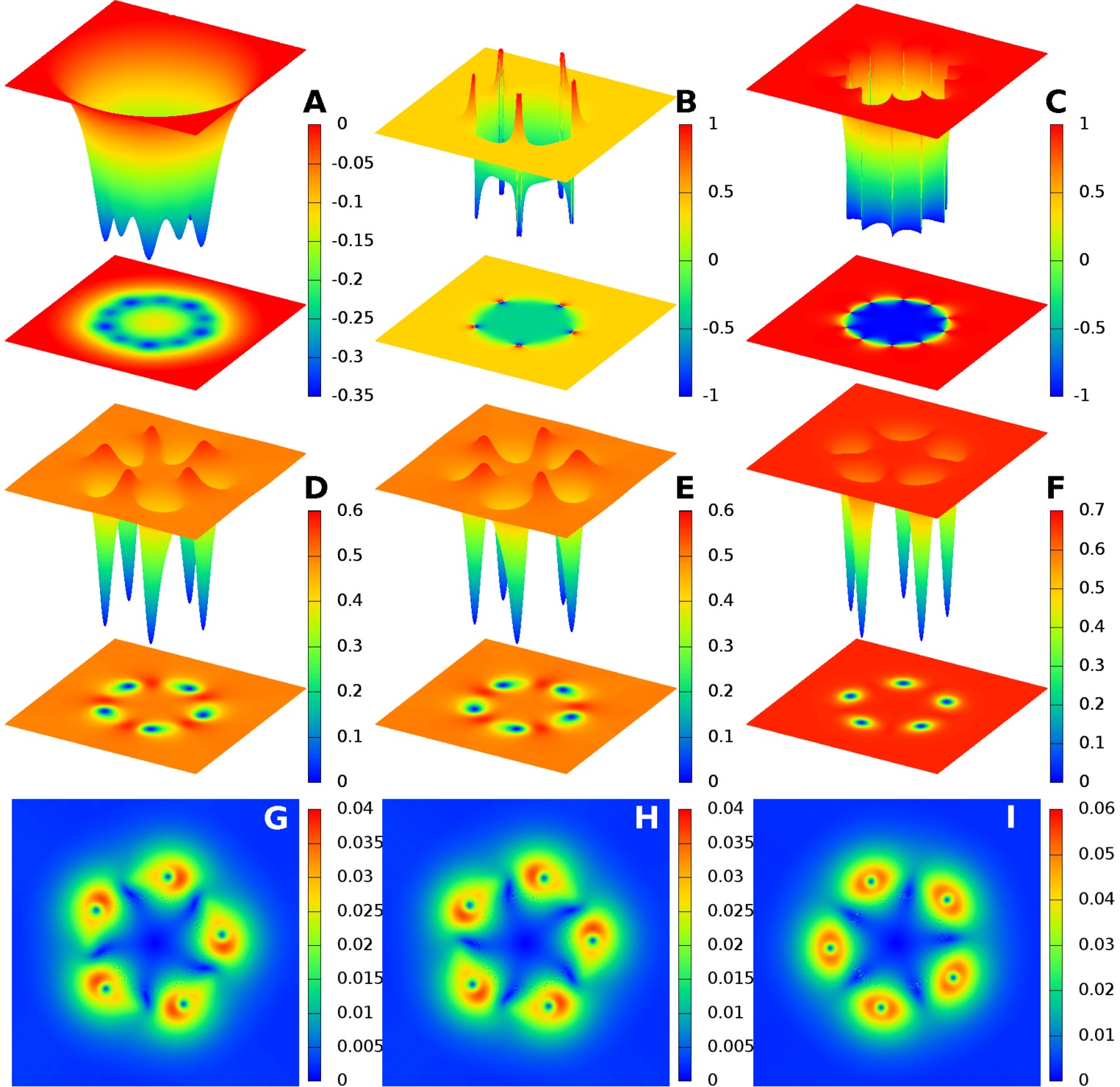
Figure 7: (Color online) – A $\mathcal{Q}=5$ quantum soliton in a system with within the same parameter set as in Fig. 6 apart from $(\alpha_{3},\beta_{3})=(-0.5,1)$. Displayed quantities are the same as in the previous pictures, e.g. Fig. 5.

Among possible observable signatures of chiral skyrmions, is the varying fraction of magnetic flux carried by fractional vortices, as in Fig. 7. There, the magnetic field exhibits spots of different magnitude, larger spots associated to the two similar bands with more density while the small spots are associated with the active band.

II.5 Chiral multi-skyrmions

Besides having non trivial $\ {\mathbbm{C}}{{P}}^{2}\$topological invariant (2.4), the chiral skyrmions in three component Ginzburg–Landau theory with BTRS have a given chirality. Namely, there is a difference whether one or the other broken ${\mathbbm{Z}}_{2}$ state is ‘inside’. Here we report bound states of chiral skyrmions with opposite chirality which can be called multi-skyrmions. More precisely a bound state of a skyrmion with a given chirality, carrying some topological charge say $\mathcal{Q}_{1}$ and a skyrmion with the opposite chirality carrying $\mathcal{Q}_{2}$, see Fig. 8. There the inner skyrmion has a smaller charge than the outer one, $\mathcal{Q}_{1}<\mathcal{Q}_{2}$ since the chiral skyrmion’s size is controlled by the number of enclosed quanta. The bigger is the difference between $\mathcal{Q}_{1}$ and $\mathcal{Q}_{2}$, the weaker is the interaction between the two chiral skyrmions. Conversely, as $\mathcal{Q}_{1}\to\mathcal{Q}_{2}$ the chiral skyrmions interact progressively more strongly. For very close values of $\mathcal{Q}_{1}$ and $\mathcal{Q}_{2}$ the chiral skyrmions falls into each other’s attractive basins and the domain walls annihilate. This allows decay to ordinary vortices.

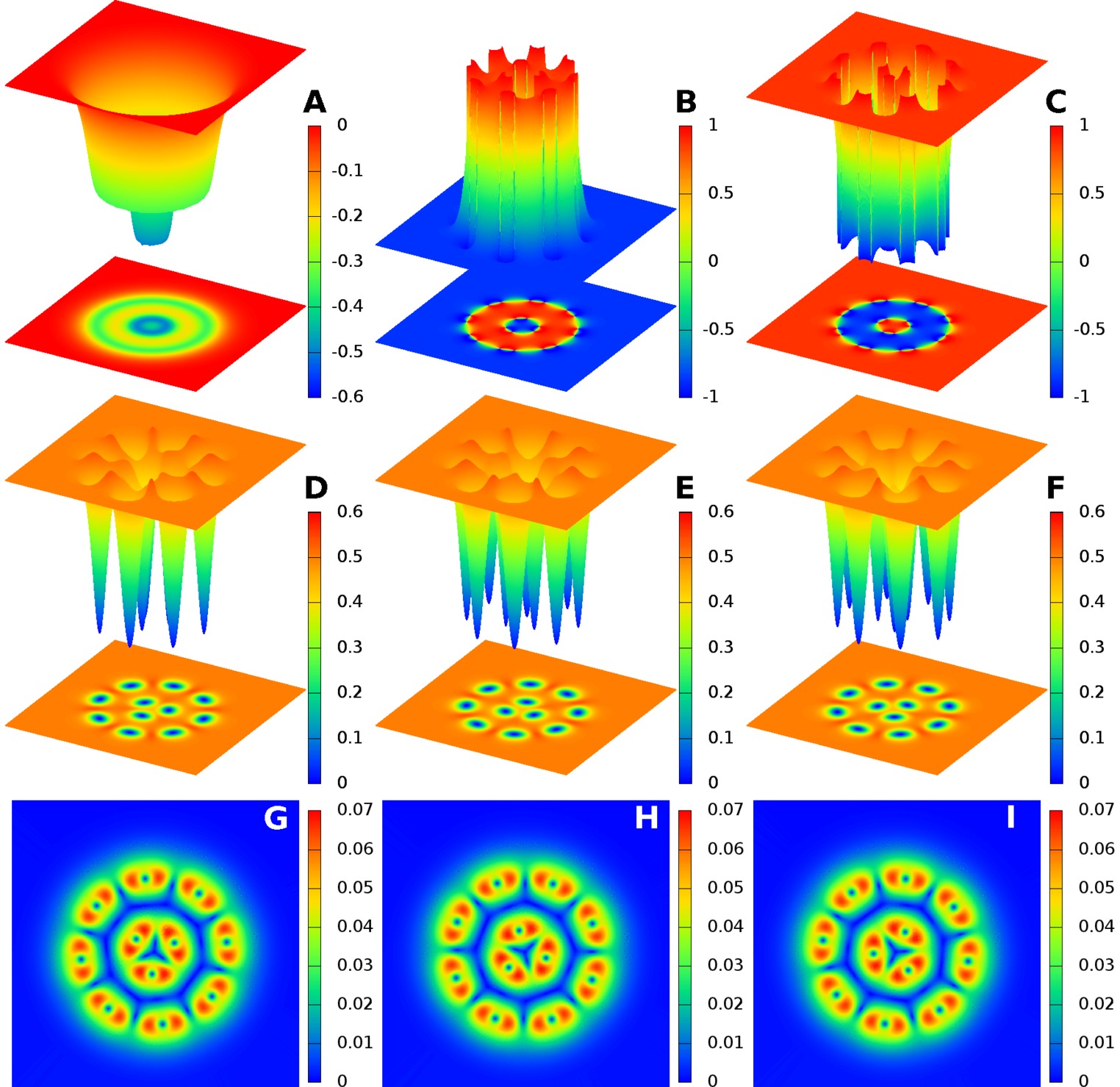
Figure 8: (Color online) – A $\mathcal{Q}=11$ quantum multi-soliton in a system with three identical passive bands as in Fig. 13. The current soliton is not made out of one but two stabilized domain walls thus being a homogeneous bi-ring configuration. Panels $(\bf B)$ and $(\bf C)$ clearly display the alternating different ground-states. Since the three bands are identical, the magnetic field rather homogeneously spreads all along the solitons. Displayed quantities are the same as in the previous pictures, e.g. Fig. 5. Note that while going counterclockwise along the outter ring, the fractional vortices have order band-”1,2,3”. For the inner ring they are ordered as band-”1,3,2”. The origin of this is discussed in Sec. IV.2

Note that “opposite chirality” should not be confused with opposite flux, i.e. these objects have opposite chirality because they interpolate between two different ${\mathbbm{Z}}_{2}$ ground states. In that respect in the BTRS case, an additional ${\mathbbm{Z}}_{2}$ topological charge like those of ordinary domain walls can be attributed to skyrmions. However having opposite ${\mathbbm{Z}}_{2}$ topological charges does not mean that these objects represent a skyrmion and an anti-skyrmion. This is because they have similar signs of $\mathcal{Q}_{1}$ and $\mathcal{Q}_{2}$ charges as well as similar signs of the total phase winding in the local $U(1)$ sector. That is, they carry magnetic flux in the same direction. For a given skyrmion one can construct an anti-skyrmion from similar number of anti-vortices. Using anti-vortices changes the overall phase winding and thus the direction of carried flux. As will be clear from the discussion below, an anti-Skyrmion with the same ${\mathbbm{Z}}_{2}$ charge as a Skyrmion will also have fractional vortices arranged in a different order.

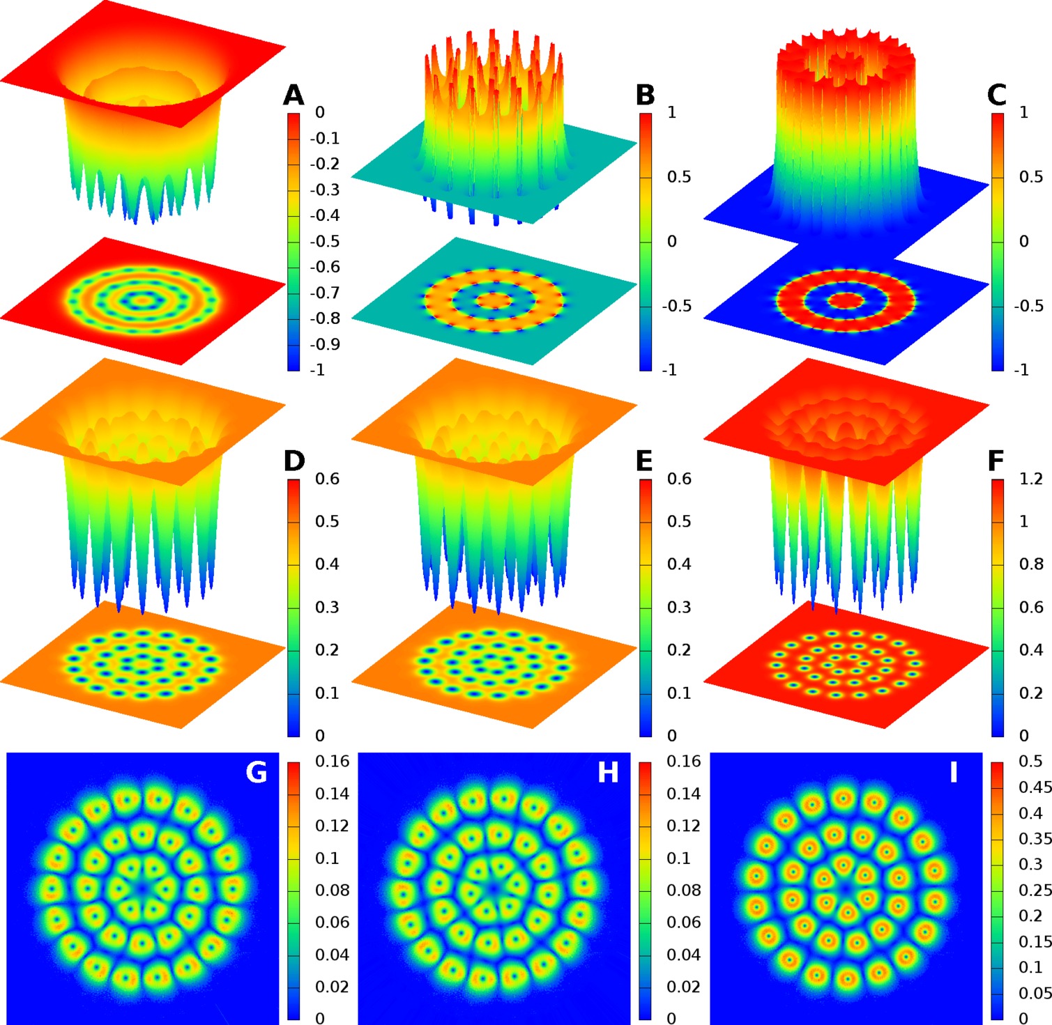
Figure 9: (Color online) – A tri-ring chiral skyrmion. The configuration carries total charge $\mathcal{Q}=36$ in a system with two identical passive bands $(\alpha_{1},\beta_{1})=(\alpha_{2},\beta_{2})=(1,1)$ coupled to a third active band with $(\alpha_{3},\beta_{3})=(-1,1)$. Josephson coupling constants are $\eta_{23}=-3$ and $\eta_{12}=\eta_{13}=1$. $e=0.7$. Panels are the same as usual, e.g. Fig. 5

Similarly, there exist also “Russian nesting doll”-like multi-skyrmions made of larger number of alternating skyrmions of opposite chiralities. Such a multiple skyrmion can be seen in Fig. 9 which shows tri-ring solutions of skyrmion with alternating chiralities. This kind of numerical solution is quite easily obtained given a good initial guess. However this configuration can also spontaneously form from ‘collisional dynamics’ of energy minimization of an initial configuration of closely spaced ordinary vortices. This indicates that formation of multi-skyrmion solutions does not in general require fine tuning. Instead these solutions have a substantial “attractive basin” in the GL energy landscape indicating they could also be observed in three component superconductors with Broken Time Reversal Symmetry.

III Physical properties of Chiral skyrmions

It is important to know the energetic properties of skyrmions compared to ordinary vortices, as well as their stability properties. Indeed if skyrmions are thermodynamically stable and form as the ground states in magnetic field, their experimental signatures are straightforward to detect. However, if they form as states with higher energy than e.g. a vortex state, they are only metastable. When they are metastable states, skyrmions are protected against decay by an energy barrier. The height of this barrier depends non-trivially on the parameters of the potential and on the number of enclosed flux quanta. Metastable chiral skyrmions could be produced by quenching the system under applied magnetic field. In this section, we discuss these aspects.

III.1 Energy of Chiral skyrmions vs vortices

For vanishing bi-quadratic density interaction couplings (i.e. $\gamma_{ab}=0$), in all the regimes which we investigated, chiral skyrmions are always more expensive energetically than vortices. However, as suggested in Ref. Garaud.Carlstrom.ea:11, , bi-quadratic density interaction decreases the energy of chiral skyrmions relative to that of vortices. For sufficiently strong bi-quadratic density interaction chiral skyrmions are ground state excitations i.e. energetically cheaper than vortices and, for certain parameters, thermodynamically stable.

The energy properties of the chiral skyrmions are displayed on the left panels of Figures 10-11. There, the energy per flux quantum of a given configuration is given in units of the single quantum flux carrying ground state. Namely $E(N)/[NE(N=1)]$ is represented as a function of $N$, the number of flux quanta. The corresponding energies are sublinear functions of enclosed flux quanta for all solutions with $N>2$. This means that the energy cost per flux quantum decreases as $N$ grows.

  

Figure 10: (Color online) – Energies per flux quantum of the skyrmions carrying $N$ flux quanta. The energy is given in units of the energy of the energetically cheapest (either vortex or skyrmion) single quantum excitation $(\bf{A})$. Middle panel $(\bf{B})$ shows $\frac{E(N)-E(N-1)}{E(N=1)}$ as a function of the number of flux quanta. When this quantity is less than one, it is energetically preferred to have a $N$-quantum skyrmion than having a $(N-1)$-skyrmion plus one isolated vortex. The criterion for thermodynamical stability $\frac{H_{c1}^{2}}{2}-|F_{\mbox{\tiny GS}}|$, where the condensation energy is $F_{\mbox{\tiny GS}}\equiv F(\langle\psi_{a}\rangle,0)$, is shown on the right panel $(\bf{C})$. Here, the dependence of the solutions on $\gamma$ and $N$ is investigated, while the gauge coupling is fixed at $e=0.3$. Other parameters are $(\alpha_{a},\beta_{a})=(1,1)$ and $\eta_{ab}=-3$. Colors and symbols associated to different values of $\gamma_{ab}$ (shown on the picture) are the same over three panels. Note that the reason why curves with high $\gamma_{ab}$ terminates for smaller $N$, is that the size of the skyrmion becomes comparable to the size of the numerical domain. To avoid any finite size effect, we chose to skip the corresponding points.

Two different regimes can be distinguished. If a configuration has $E(N)/[NE(N=1)]>1$ (where $E(N=1)$ is the energy of a single vortex), then it is energetically preferable to have $N$ isolated type-II integer flux vortices. As discussed below, there, skyrmions should be understood as metastable objects. That is, they can decay into type-II (composite) vortices, e.g. in case of strong enough perturbations. On the other hand, when $E(N)/[NE(N=1)]<1$, then isolated vortices are no longer energetically preferred over a skyrmion. In the first case, (corresponding to the upper curves of Fig. 10), chiral skyrmions can exist as meta-stable excitations. In the second situation (the lower curves of Fig. 10), chiral skyrmions could form as true ground state topological excitations. Note also that there is a regime where lower charge skyrmions are more expensive than type-II integer vortices, while higher charge ones are cheaper (see Fig. 10). In the regimes where there is density-density interaction, even the smallest skyrmions with $\mathcal{Q}=N=1$ can be energetically cheaper than vortices.

The relative cost of including an additional flux quantum into a chiral skyrmion is evaluated by computing $\frac{E(N)-E(N-1)}{E(N=1)}$. When this quantity is less than one, it is globally beneficial to merge an additional flux-quantum-carrying object with a skyrmion. It is displayed on panel $(\bf{B})$ of Figures 10-11. Note that it does not tell about the real work the system has to provide for bringing the isolated single quantum defect from infinity into the skyrmion, but only on global cost or benefit.

III.2 Thermodynamical stability of Chiral skyrmions

The first critical field is defined as the applied magnetic field at which the formation of a single flux carrying defect (vortex or skyrmion) becomes energetically favorable. It is defined in analogy with the first critical field for ordinary vortices $H_{c1}=E_{d}/\Phi_{d}$, where $E_{d}$ and $\Phi_{d}$ are the energy and magnetic flux of the topological defect $E_{d}=\int(\mathcal{F}(\psi_{a},\boldsymbol{A})-\mathcal{F}_{\mbox{\tiny GS}})$ and $\mathcal{F}_{\mbox{\tiny GS}}\equiv\mathcal{F}(\langle\psi_{a}\rangle,0)$ is the ground state energy. I.e. it is energetically preferred to form a topological defect carrying flux $\Phi_{d}$ in external field $H_{0}$ if the Gibbs free energy $E_{d}-\Phi_{d}H_{0}<0$. The external field $H_{0}$ should be smaller than the thermodynamical critical magnetic field $H_{ct}=2\sqrt{\mathcal{F}(0,0)-\mathcal{F}_{\mbox{\tiny GS}}}$. The criterion for thermodynamical stability is investigated on the right panels $(\bf{C})$ of Figures 10-11. For all these regimes, $\frac{H_{c1}^{2}}{2}-|\mathcal{F}_{\mbox{\tiny GS}}|<0$. In all displayed cases, skyrmions satisfy this criterion. That means that under certain conditions they can be induced by an applied external field.

  

Figure 11: (Color online) – Energies per flux quantum of the chiral skyrmions, in the units of the energy of the energetically cheapest (either vortex or skyrmion) single quantum excitation $(\bf{A})$. Curves with same color and symbols on different panels have same parameters. The middle panel $(\bf{B})$ shows that it is always beneficial (within a parameter range) to have a higher charge skyrmion than a lower charge one plus an isolated one quantum vortex. The criterion for thermodynamical stability of $N$-quantum solitons $\frac{H_{c1}^{2}}{2}-|\mathcal{F}_{\mbox{\tiny GS}}|$, where $\mathcal{F}_{\mbox{\tiny GS}}\equiv\mathcal{F}(\langle\psi_{a}\rangle,0)$ is the condensation energy $(\bf{C})$. The dependence of the solutions on $e$ and $N$ is investigated, for a strength of the density-density interactions $\gamma_{ab}=0.8$. Other parameters are the same as in Fig. 10. Here again curves are truncated when the soliton’s size becomes comparable to the numerical domain.

III.3 Perturbative stability of Chiral skyrmions

 

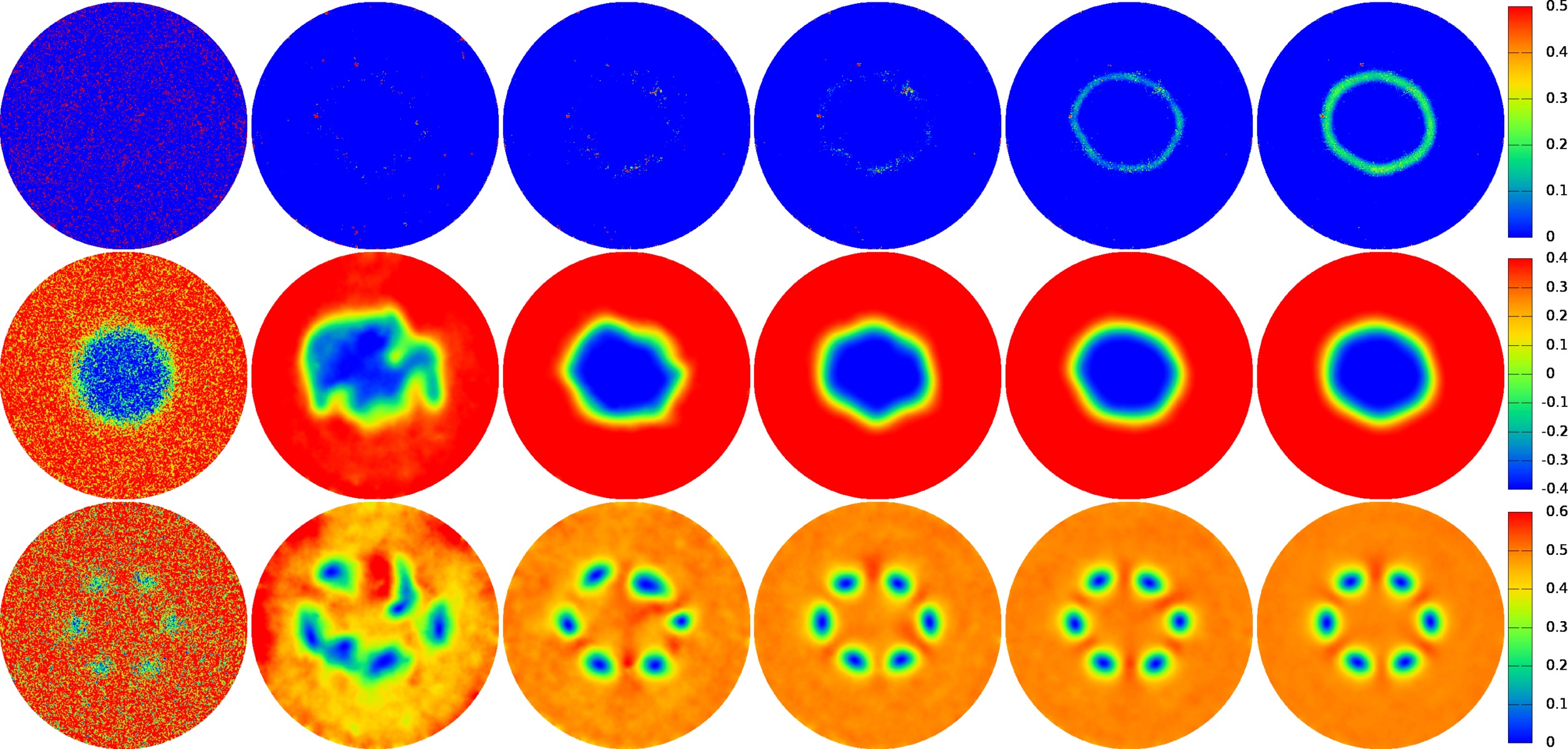
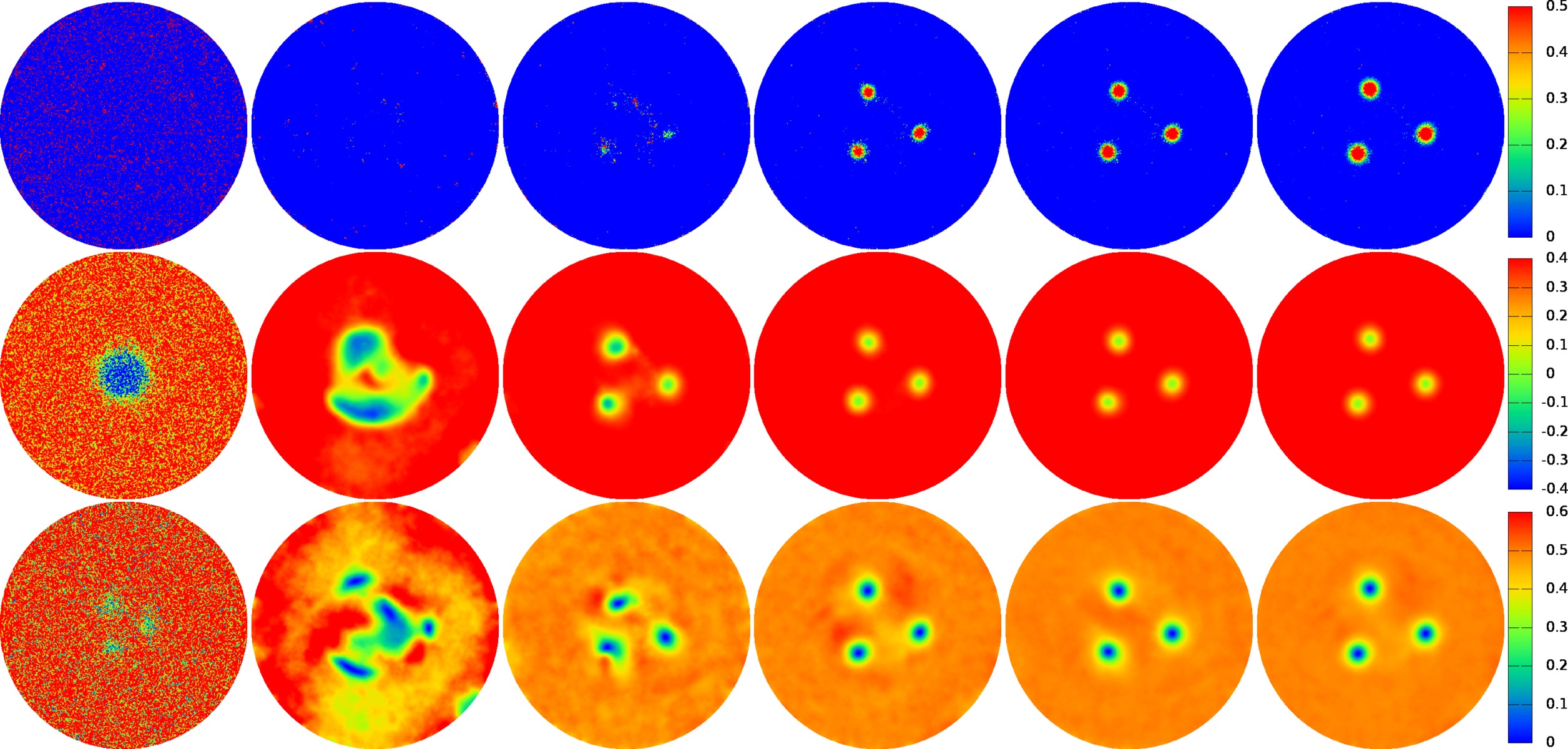
Figure 12: (Color online) – Relaxation of a randomly perturbed chiral skyrmion. Displayed quantities are the energy density, $\mathrm{Im}(\psi_{1}^{*}\psi_{2})$ and $|\psi_{1}|^{2}$. The parameters are the same as in Fig. 3, but vanishing bi-quadratic density interactions $\gamma_{ab}=0$ and $e=0.3$. Thus it is only meta-stable. The snapshots show the state of the system at different stages of the energy minimization algorithm after the applied perturbation. On the top panel, a $\mathcal{Q}=6$ chiral skyrmion with initial white noise of 70 % of the ground state values. The configurations relaxes to a chiral skyrmion. On the bottom panel, a perturbation of a metastable charge $\mathcal{Q}=3$ soliton with an initial noise $P=0.8$. Here, the noise is strong enough to break up the domain wall. The soliton thus relaxes to ordinary type-II vortices (one can clearly see the disappearance of the domain wall between blue and red area in the middle row). The last snapshot in the lower configuration does not represent a stationary configuration: the vortices repel each other and are in process of drifting apart.

Chiral skyrmions can appear as thermodynamically stable ground states or metastable states in superconductors with Broken Time Reversal Symmetry. In this work, they are obtained by minimizing the energy. Consequently, they are always minima (at least local) of the free energy landscape. When the chiral skyrmions are metastable states they are protected against decay into type-II vortices by a finite energy barrier. The analysis carried out in this subsection concerns the metastable solutions. In all the regimes which we considered, metastable chiral skyrmions are found to be very robust. They are easily formed during the energy minimization, e.g. in closely spaced groups of vortices. The energy barrier preventing them from decay to type-II vortices is typically quite high. Although difficult to quantify, it is interesting to have a qualitative insight into the behaviour of metastable skyrmions against fluctuations.

One possible approach to study the stability of skyrmions is the linear stability analysis which consists of applying infinitesimally small perturbation to the fields, and investigating the eigenvalue spectrum of the (linear) perturbation operator, on the background of a given solution. When the background solution is (meta) stable all infinitesimally small perturbations are positive modes and thus can only increase the energy. As a result linear stability analysis cannot tell anything especially interesting about the properties of skyrmions. A strong perturbation should cause a decay of a metastable chiral skyrmion to ordinary vortices. Here, the stability is investigated numerically by perturbing the chiral skyrmion by white noise. This allows one to investigate the full non-linear response where the meaningful information belongs. The white noise applied to all degrees of freedom, is generated as follows

$$\psi_{a} =\psi_{a}^{(0)}+P\mathrm{max}(|\psi|)\mu_{a}^{\mbox{\tiny$\psi$}}(x,y)\,,$$

$$A_{i} =A_{i}^{(0)}+P\mathrm{max}(|\boldsymbol{A}|)\mu_{i}^{\mbox{\tiny$\boldsymbol{A}$}}(x,y)\,.$$ (3.11)

Here ⁽⁰⁾ denotes the fields of the initial skyrmionic state, $P$ is a ratio giving the relative magnitude of the perturbation with respect to the maximal amplitude of a given field of the initial state. $\mu_{a}^{\mbox{\tiny$\psi$}}(x,y)$, and $\mu_{i}^{\mbox{\tiny$\boldsymbol{A}$}}(x,y)$ are (independent) random functions of the space. They satisfy $|\mu_{a}^{\mbox{\tiny$\psi$}}|<1$ and $|\mu_{i}^{\mbox{\tiny$\boldsymbol{A}$}}|<1$. As a result all fields initially receive a noise whose relative amplitude is $P$. The perturbation has very large field gradients since it is applied locally on the mesh. After applying noise the system is then relaxed using the same minimization scheme as for constructing the skyrmions. Despite the strong field gradients, if the white noise does not exceed a certain threshold, the configuration relaxes back to the initial chiral skyrmion solution. This can be seen from the upper panel of Fig. 12. The noise was gradually increased, confirming that indeed, a sufficiently strong perturbation drives the metastable solution over the barrier, in the energy landscape, thus leading to its decay to ordinary vortex solutions as shown on the bottom panel of Fig. 12. The precise value of the relative amplitude required to destabilize a given chiral skyrmion, obviously depends on the parameters of the Ginzburg–Landau functional and on the number of flux quanta of the solution.

As expected, if a perturbation is strong enough, the metastable chiral skyrmion decays to the configuration with less energy, i.e. isolated type-II vortices. The observed behaviour confirms the expectations from energy arguments Sec. III.1. Moreover, the deeper in the type-II regime, the less breakable are the skyrmions. One of the easiest ways for a skyrmion to decay is to deform it enough so that the domain wall self intersects. The configuration then can decay to skyrmionic configurations with lower $\mathcal{Q}$ which are less stable and can further decay into integer vortices.

IV Interactions of Chiral skyrmions

The analysis of the energetic properties of chiral skyrmions suggests they should have quite non trivial interactions. Generally, the energy per flux quantum decreases with the topological charge (see e.g. Fig. 10). In some cases it is also preferable to absorb isolated vortices into a skyrmion, i.e. the energy of an $N$-quantum vortex is less than that of an $(N-1)$-quantum vortex and an isolated vortex. In those cases, the interaction at short range should be attractive. On the other hand, they exist in regimes where vortices usually exhibit repulsive interaction (type-II or even type-1.5). Moreover, the lack of axial symmetry and complicated internal structure featuring fractional vortices can provide very non-trivial contribution to the interaction of skyrmions in BTRS superconductors.

IV.1 Chiral skyrmion–vortex interaction

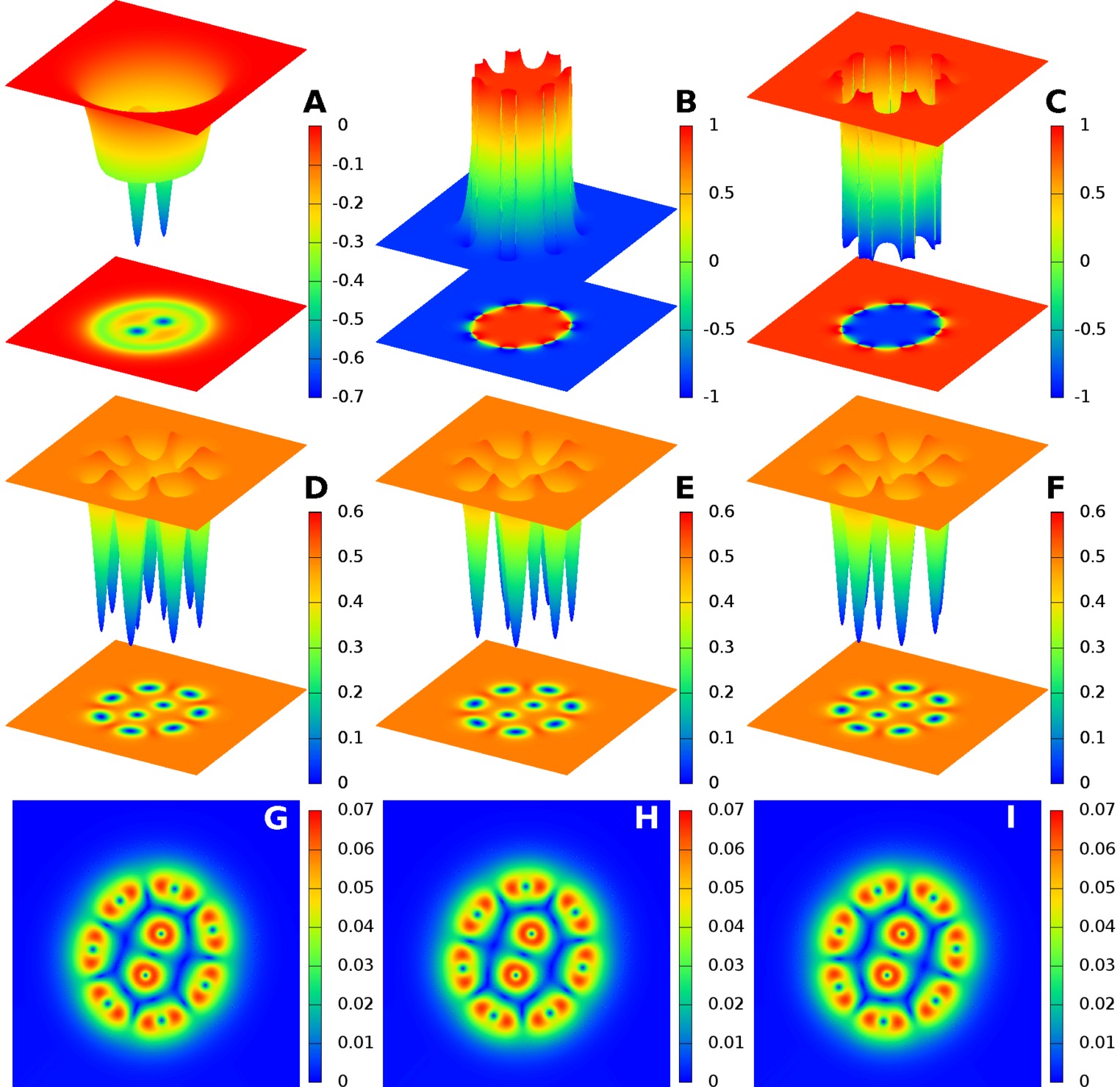
Figure 13: (Color online) – A $\mathcal{Q}=9$ quantum configuration of mixed vortices and skyrmions in a system with three identical passive bands as in Fig. 12. This configuration is made out of a skyrmion surrounding two ordinary vortices. It is known, from energy considerations that interaction is short range attractive. Interaction with vortices deforms the skyrmions. This shows that it is long range repulsive.

Chiral skyrmions can have very non trivial, non-monotonic interaction with vortices. As seen from the numerically obtained solutions shown on Fig. 10 and Fig. 11, in applied field, chiral skyrmions can be either ground states (for a given phase winding) or represent metastable states. For some regimes, as seen from the middle panels of Fig. 10 and Fig. 11, a vortex placed sufficiently close to a chiral skyrmion should be absorbed in the domain wall and split into fractional vortices, thus increasing the charge of the skyrmion and then decreasing its energy per flux quantum. Consequently, the interaction is expected to be attractive at short range. Indeed, as we observe in numerical calculations, if vortices are placed close enough to a domain wall, they are easily trapped to form a skyrmion of larger topological charge. However the long range forces between skyrmions and vortices can be repulsive. This is clearly seen from the existence of stable configurations where a number of integer flux vortices are confined within a chiral skyrmion, as shown on Fig. 13. That figure demonstrates that there is a repulsion between inner “ordinary vortices”, and the fractional vortices comprising the chiral skyrmion, which follows from (i) the stability of the configuration and (ii) the fact that the type-II vortices visibly stretch the skyrmion. Thus the interaction here is non-monotonic, being long range repulsive, but short range attractive.

The repulsive long-range skyrmion-vortex interaction follows from the following considerations. In the ground state a vortex is an axially symmetric object with all phases winding around the same core. Thus in the type-II limit its energy and long-range interactions are dominated by the supercurrent $\bf J$ term in (2.5a). At long separations when linearized theory applies, the interaction between a skyrmion and a vortex is dominated by this current-current $\bf J$-mediated interaction, resulting in repulsion. The attractive interaction at short distances is a nonlinear effect where split fractional vortices in a Skyrmion can deform a vortex by “polarizing” it. i.e. they can split its constituent fractional vortices thus inducing “dipole”-like interactions. This interaction attracts the vortex so that it merges into the skyrmion.

IV.2 Skyrmion–skyrmion interaction

In contrast to ordinary vortices in Ginzburg–Landau theory, chiral skyrmions do not exhibit rotational symmetry. An important consequence is that inter-soliton interactions should in general depend on the relative orientation of the solitons. First, note that the orientation and position of a soliton can be described by the position of the fractional vortices. The shape of a soliton, including the positions of the constituting fractional vortices is determined by energy minimization. The energy of the skyrmion is invariant under overall rotation and translation.

Finally note that there are two orders in which the fractional vortices can be arranged. Going counter-clockwise along the domain wall, the vortices can be ordered $1,2,3$ or $1,3,2$. We denote this order $o=\epsilon_{abc}$, $\epsilon$ being the Levi-Civita symbol and $a,b,c$ are the band indices of the fractional vortices. For a skyrmion carrying integer flux, $o=\pm 1$ (note that this ordering closely relates to the concept of chirality). As illustrated in Fig. 14 (a), a system of two solitons is thus described by the distance between them $R$, their relative orientation $v$ together with the ordering (chirality) of each individual skyrmion.

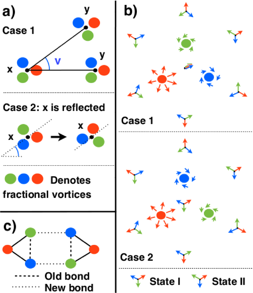
Figure 14: (Color online) – Panel (a) shows a schematic picture of how soliton interactions are computed. This figure shows the interaction between two single quanta solitons, each consisting of three fractional vortices shown in green, blue and red. This generalizes easily to larger solitons. One soliton ($\rm x$) is placed in the origin, while the second ($\rm y$) is placed at a distance $R$ at an angle $v$. Consequently, as $v$ is varied, the relative orientation of the solitons changes. Case 1 shows a system of two solitons with identical chiralities (same ordering $o$), while case 2 shows two solitons with opposite chiralities (different $o$), although the mirrored soliton is not necessarily stable. A schematic comparison of solitons with different ordering $o$ is displayed on panel (b). In the case (2), the gradients in phase difference due to the fractional vortices naturally interpolate between two ${\mathbbm{Z}}_{2}$ states. For this reason, the case (2) is energetically preferable over (1) and it was verified numerically. Finally, panel (c) gives a schematic view of the merging of two single quanta solitons. In order to merge, they should have same ordering but opposite orientation.

IV.2.1 Chirality of skyrmions: inequivalence of left- and right- handed solutions

In general, for a chiral skyrmion, the energy is not independent of the ordering $o$. For a given ${\mathbbm{Z}}_{2}$ ground state outside of a skyrmion, the system allows only one particular ordering $o$ of the fractional vortices in the skyrmion. The mechanism that gives rise to this behaviour is illustrated in Fig. 14 (b): For a given external phase-locking pattern (a ${\mathbbm{Z}}_{2}$ state), only a particular ordering $o$ gives the opposite ${\mathbbm{Z}}_{2}$ state inside. In the illustration the two solitons (case 1 and 2) differ in the ordering of the fractional vortices (represented by red blue and green dots with band index 1,2,3 respectively) – the corresponding phase configurations are shown by the arrows. Thus, the ordering of the first one (case 1) is $o=\epsilon_{132}=-1$ while the ordering of the second (case 2) is $o=\epsilon_{123}=+1$. Now for a same given ground state outside both solitons, the phase-locking inside is determined consistently with the phase gradients of each fractional vortex. In the first case, it results in a phase arrangement inside the soliton that is not a ground state. However, in the second case, the state obtained inside is a different ${\mathbbm{Z}}_{2}$ ground-state. As a result, there is a synergy effect where the phase gradients due to the fractional vortices go from one ${\mathbbm{Z}}_{2}$ state to another. Therefore $o=+1$ is energetically cheaper than $o=-1$ for which the inner phase locking is the farthest from the ground state. This is indeed confirmed in our numerical simulations where a skyrmion $o=-1$ decays into a skyrmion $o=+1$. Thus the ordering of the fractional vortices does matter in BTRS superconductors. It results in the discrimination of one ordering. This further motivates the terminology chiral.

IV.2.2 Numerical calculations on inter-skyrmion forces

As illustrated in Fig. 14 (a), inter-soliton forces are computed according to the following procedure. First, the structure of the soliton is determined by unconstrained energy minimization, thus determining the actual position of the fractional vortices constituting the skyrmion. Then two skyrmions ($\rm x$ and $\rm y$ in Fig. 14) are place at a distance $R$ and a relative orientation $v$. There, the energy is minimized with respect to all degrees of freedom, except the position of the singularities of each fractional vortex. As shown in Fig. 14 (a), the energy is computed for every distance and relative orientation $R$ and $v$. While allowing computation of long-range inter soliton forces, this procedure has an important limitation. It does not take into account one of the nonlinear effects: Deformation of interacting solitons in the form of changes of the position of the fractional vortices. However, this is primarily a problem at short separation, where the deformation is generally the strongest.

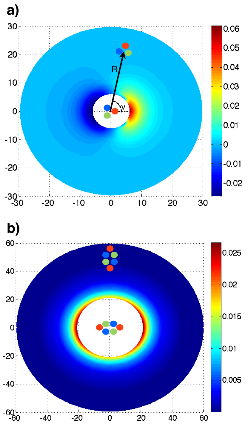
Figure 15: (Color online) – Panel (a) displays the interaction energy of two single quantum skyrmions. One soliton is placed at the origin, the interaction energy is plotted as a function of the position and relative orientation of the second soliton. The interaction energy is maximal when $v=0$ while it is minimal for the opposite orientation, $v=\pi$. The strength of the interaction decreases with the separation $R$. The model parameters are the same as in Fig. 3. Panel (b) shows the interaction energy of two $\mathcal{Q}=2$ quanta solitons, for the same parameters as in Fig. 5. Note that the skyrmion has two-fold symmetry (it is invariant under global rotations of $\pi$). The minimum energy is found for the relative orientation $v\pm\pi/2$.

Fig. 15 (a) shows the interaction energy of two single quanta skyrmions, identical to the one in Fig. 3. From Fig. 11 it is clear that the energy per flux quanta decreases with the number of flux quanta. For the solitons to merge, they need to have opposite orientation, see Fig. 14 (c). The computed interaction energy, Fig. 15 (a), is indeed consistent with this picture. When the relative orientation, $v$ is not optimal i.e. $v\not=\pi$, the solitons exert a torque on each other, so that they attain this optimal orientation. Then, an attractive channel opens in the potential, allowing them to get closer where nonlinear effects are strong, ultimately leading to a merger.

The interaction energy of a slightly more complex soliton is shown in Fig. 15 (b). There, each skyrmion carries two flux quanta (i.e. their topological charge is $\mathcal{Q}=2$). The parameters are the one of Fig. 5, from which we know that superconducting components are not identical and that the skyrmion is more or less elliptic. Global orientation of the skyrmion is chosen so that when $v=0$ the major axis of both solitons lie along the horizontal axis. Note that these skyrmions are not only invariant under global rotation by $2\pi$, but also by $\pi$. Within the numerical accuracy, the inter-skyrmion interaction is always repulsive. Note that this approach can accurately determine the interaction only at sufficiently long distances. Indeed, by fixing the positions of the fractional vortices, it assumes that the skyrmions are almost-rigid bodies. The relative position of singularities in each fractional vortex is fixed once for all, but the fields can deform around this rigid ‘skeleton’. This neglects the possibility of mutually induced deformations of the ‘skeleton’, which can open an attractive channel. Since our “almost-rigid body” approximation holds only at large enough distances, short range data are irrelevant and not displayed in Fig. 15. We also derive general long-range intersoliton forces in the more formal framework of Sec. V.3. In Sec. V.5 the formal long-range interactions are applied to the particular case of a BTRS superconductor. The predictions derived there are consistent with the numerical results presented in this section.

V Mathematical analysis of long-range intersoliton forces

The model considered in this paper has many properties that are interesting from a formal, mathematical point of view. In this section we show how, by re-writing the free energy in terms of gauge-invariant fields, we can identify a hidden topological charge, associated with the topology of the complex projective space ${\mathbb{C}}{{P}}^{2}$, and devise a mathematically satisfactory scheme for deducing the nature (attractive or repulsive) and range of the dominant force between well-separated solitons (either vortices or skyrmions). For generic parameter choices, the final step in this scheme (finding the spectrum of a symmetric real matrix) must be done numerically, but there are several symmetric cases and parametric limits where all calculations can be completed explicitly. After treating the general case, we consider two such special cases, both of potential phenomenological interest.

V.1 Reduction to a supercurrent coupled ${\mathbb{C}}{{P}}^{k-1}$ model

In this section we consider a general $k$ component GL model, with no restriction on the potential terms $V$. The $k$ complex fields $\psi_{a}$ may be collected into a complex $k$-vector $\Psi:M\rightarrow{\mathbb{C}}^{k}$, where $M={\mathbb{R}}^{2}$ denotes physical space. It is convenient to use polar coordinates on ${\mathbb{C}}^{k}$ by defining

$$\Psi=:\rho Z$$ (5.12)

where $\rho=\sqrt{\Psi^{\dagger}\Psi}\geq 0$ and $Z^{\dagger}Z=1$. Let $\pi:{\mathbb{C}}^{k}\backslash\{0\}\rightarrow{\mathbb{C}}{{P}}^{k-1}$ denote the canonical projection which takes a point in ${\mathbb{C}}^{k}$ to the complex line through $0$ containing that point, and for any $X\in{\mathbb{C}}^{k}$, $X\neq 0$, denote by $[X]$ its projective equivalence class (so $[X]=\pi(X)$). By gauge invariance, the potential $V(\Psi)$ can actually depend only on $\rho$ and $[Z]\in{\mathbb{C}}{{P}}^{k-1}$, the projective equivalence class of $Z$, or, equivalently, of $\Psi$. Let $\Phi=\pi\circ\Psi$. This is a ${\mathbb{C}}{{P}}^{k-1}$-valued field which maps each $p\in M$ to $[\Psi(p)]=[Z(p)]\in{\mathbb{C}}{{P}}^{k-1}$. By construction it is, like $\rho$, gauge invariant. We may rewrite the free energy entirely in terms of the gauge-invariant quantities $\rho,\Phi$ and $J=e\mathrm{Im}(\Psi^{\dagger}D\Psi)$, the total supercurrent. To do so, it is convenient to think of the gauge field $A$ and the supercurrent $J$ as one-forms rather than vector fields (so we use the metric on physical space $M={\mathbb{R}}^{2}$ to “lower the indices” on vectors $A^{i}$ and $J^{i}$). In this language, the covariant derivative of $\Psi$ is, likewise, a one-form

$$D\Psi=\mathrm{d}\Psi+ieA\Psi$$ (5.13)

with values in ${\mathbb{C}}^{k}$.

On ${\mathbb{C}}^{k}\backslash\{0\}$, let us define the real one-form

$$\nu=-{\rm Im}\frac{X^{\dagger}\mathrm{d}X}{|X|^{2}}.$$ (5.14)

where $X=(X_{1},\ldots,X_{k})$ is a global coordinate on ${\mathbb{C}}^{k}\backslash\{0\}$ and $\mathrm{d}X=(\mathrm{d}X_{1},\ldots,\mathrm{d}X_{k})$ are the corresponding holomorphic one-forms. Then the total supercurrent is

$$J=e\rho^{2}\{eA-\Psi^{*}\nu\}$$ (5.15)

where $\Psi^{*}\nu$ denotes the pullback of $\nu\in\Omega^{1}({\mathbb{C}}^{k}\backslash\{0\})$ to $M$ by the map $\Psi:M\rightarrow{\mathbb{C}}^{k}\backslash\{0\}$. In less compact notation, this is the one-form on $M$ whose $\mathrm{d}x^{i}$ component is $-\rho^{-2}{\rm Im}\Psi^{\dagger}\partial_{i}\Psi$. It follows that the magnetic field (thought of as a two-form) is

$$B=\mathrm{d}A=\frac{1}{e}\left(\mathrm{d}(\Psi^{*}\nu)-\frac{1}{e}\mathrm{d}\left(\frac{J}{\rho^{2}}\right)\right).$$ (5.16)

It is a general fact that the exterior differential operator $\mathrm{d}$ commutes with pullback of differential forms, so $\mathrm{d}(\Psi^{*}\nu)=\Psi^{*}(\mathrm{d}\nu)$. Note that $\mathrm{d}\nu$ is a closed two-form on ${\mathbb{C}}^{k}\backslash\{0\}$. Let $h$ denote the Fubini-Study metric on ${\mathbb{C}}{{P}}^{k-1}$ with constant holomorphic sectional curvature $1$, and $\omega$ denote its associated kähler form. Then the pullback of $\omega$ by $\pi:{\mathbb{C}}^{k}\backslash\{0\}\rightarrow{\mathbb{C}}{{P}}^{k-1}$ is, like $\mathrm{d}\nu$, a closed two-form on ${\mathbb{C}}^{k}\backslash\{0\}$. In fact, $\omega$ is defined kobnom by the requirement that

$$\pi^{*}\omega=2\mathrm{d}\nu.$$ (5.17)

Hence

$$\mathrm{d}(\Psi^{*}\nu)=\Psi^{*}(\mathrm{d}\nu) =\frac{1}{2}\Psi^{*}(\pi^{*}\omega)$$

$$=\frac{1}{2}(\pi\circ\Psi)^{*}\omega=\frac{1}{2}\Phi^{*}\omega,$$ (5.18)

and so

$$B=\frac{1}{e}\left(\frac{1}{2}\Phi^{*}\omega-\frac{1}{e}\mathrm{d}\left(\frac{J}{\rho^{2}}\right)\right).$$ (5.19)

Similarly, we may rewrite $|D\Psi|^{2}$ entirely in terms of the gauge invariant quantities $\rho,\Phi$ and $J$. From (5.15), we see that

$$D\Psi =\mathrm{d}\Psi+i\left(\Psi^{*}\nu-\frac{J}{e\rho^{2}}\right)\Psi$$

$$=(\mathrm{d}\rho)Z+\rho\mathrm{d}Z+i\left(\Psi^{*}\nu-\frac{J}{e\rho^{2}}\right)\rho Z.$$ (5.20)

Let $e_{1},e_{2}$ denote an orthonormal frame on $M$ (for example $e_{i}=\partial/\partial x^{i}$) and $X_{i}=\mathrm{d}Z(e_{i})\in T_{Z}S^{2k-1}$. Then $\mathrm{Re}(Z^{\dagger}X_{i})=0$ since $X_{i}$ is tangent to the unit sphere in ${\mathbb{C}}^{k}$ at $Z$. Hence

$$|D\Psi|^{2} =\sum_{i}(D\Psi(e_{i}))^{\dagger}D\Psi(e_{i})$$

$$=\sum_{i}\Bigg{\{}(\mathrm{d}\rho(e_{i}))^{2}+\rho^{2}|X_{i}|^{2}$$

$$\quad+2\mathrm{Im}(X_{i}^{\dagger}Z)\rho^{2}\left(\frac{J(e_{i})}{e\rho^{2}}-\Psi^{*}\nu(e_{i})\right)$$

$$\quad+\rho^{2}\left(\frac{J(e_{i})}{e\rho^{2}}-\Psi^{*}\nu(e_{i})\right)^{2}\Bigg{\}}$$

$$=|\mathrm{d}\rho|^{2}+\frac{1}{e^{2}\rho^{2}}|J|^{2}+\rho^{2}\sum_{i}(|X_{i}|^{2}-\nu(X_{i})^{2})$$ (5.21)

since $\mathrm{Im}(X_{i}^{\dagger}Z)=\nu(X_{i})=(\Psi^{*}\nu)(e_{i})$. Consider $\pi^{*}h$, the pullback by $\pi$ of the Fubini-Study metric on ${\mathbb{C}}{{P}}^{k-1}$ to ${\mathbb{C}}^{k}\backslash\{0\}$. Given any tangent vector $X\in T_{Z}S^{2k-1}$,

$$(\pi^{*}h)(X,X) =h(\mathrm{d}\pi X,\mathrm{d}\pi X)=\omega(\mathrm{d}\pi X,i\mathrm{d}\pi X)$$

$$=\omega(\mathrm{d}\pi X,\mathrm{d}\pi iX)=\pi^{*}\omega(X,iX)$$

$$=2\mathrm{d}\nu(X,iX)=4(|X|^{2}-\nu(X)^{2})$$ (5.22)

where we have used the fact that $\pi:{\mathbb{C}}^{k}\backslash\{0\}\rightarrow{\mathbb{C}}{{P}}^{k-1}$ is holomorphic (so $\mathrm{d}\pi$ commutes with $i$). Hence

$$\sum_{i}(|X_{i}|^{2} -(\Psi^{*}\nu)(e_{i})^{2})=\frac{1}{4}\sum_{i}\pi^{*}h(X_{i},X_{i})$$

$$=\frac{1}{4}\sum_{i}\pi^{*}h(\mathrm{d}\Psi e_{i},\mathrm{d}\Psi e_{i})$$

$$=\frac{1}{4}\sum_{i}h(\mathrm{d}\Phi e_{i},\mathrm{d}\Phi e_{i})=\frac{1}{4}|\mathrm{d}\Phi|^{2},$$ (5.23)

where $|\mathrm{d}\Phi|$ denotes the norm of the linear map $\mathrm{d}\Phi_{p}:T_{p}M\rightarrow T_{\Phi(p)}{\mathbb{C}}{{P}}^{k-1}$ with respect to the metric $h$. Substituting (5.23) into (V.1), one sees that

$$|D\Psi|^{2}=|\mathrm{d}\rho|^{2}+\frac{|J|^{2}}{e^{2}\rho^{2}}+\frac{\rho^{2}}{4}|\mathrm{d}\Phi|^{2}.$$ (5.24)

Finally, we obtain an expression for the total free energy

$$F= \int_{M}\Bigg{\{}\frac{1}{2}|\mathrm{d}\rho|^{2}+\frac{\rho^{2}}{8}|\mathrm{d}\Phi|^{2}+\frac{|J|^{2}}{2e^{2}\rho^{2}}$$

$$+\frac{1}{2e^{2}}\left|\mathrm{d}\left(\frac{J}{e\rho^{2}}\right)-\frac{1}{2}\Phi^{*}\omega\right|^{2}+V(\rho,\Phi)\Bigg{\}}.$$ (5.25)

The above expression for $F$ is valid for any number of condensates $k$, and for all field configurations where $\Psi^{-1}(0)\subset M$ has measure zero, i.e. where the set of points in physical space at which the condensates $\psi_{a}$ all simultaneously vanish is negligible. This condition holds for skyrmions ($\Psi^{-1}(0)$ is empty), and for (multi-)vortices ($\Psi^{-1}(0)$ is finite), so we can use (V.1) for questions involving either type of soliton, though one should note that, for vortices, the ${\mathbb{C}}{{P}}^{k-1}$-valued field $\Phi$ is undefined at the finite collection of vortex positions.

In the special case $k=2$, we may identify ${\mathbb{C}}{{P}}^{k-1}$ with the unit two-sphere $S^{2}$ , by mapping $[Z_{1},Z_{2}]\in{\mathbb{C}}{{P}}^{1}$ to the point on $S^{2}$ with stereographic coordinate $Z_{2}/Z_{1}$, so that $\Phi$ can be interpreted as being two-sphere valued. The kähler form $\omega$ coincides with the area form on $S^{2}$ under this identification, so that the expression for $F$ (V.1) reduces to the decomposition in Ref. bfn, . In the general $k$ case (which was previously discussed, in somewhat different mathematical language, in context of an $SU(N)$ model in Ref. Hindmarsh:93, ), the field $\Phi$ takes values in ${\mathbb{C}}{{P}}^{k-1}$, which we cannot identify with any sphere.

V.2 Flux quantization and the topological charge

In order for a configuration on $M={\mathbb{R}}^{2}$ to have finite total energy, $\Phi$ and $\rho$ should tend to constants $\Phi_{0}\in{\mathbb{C}}{{P}}^{k-1}$, $\rho_{0}\in(0.\infty)$, and $J$ should tend to $0$ as $|x|\rightarrow\infty$. It follows, from (5.19) and Stokes’s theorem, that the total magnetic flux of a finite energy configuration is

$$\int_{M}B=\frac{1}{2e}\int_{M}\Phi^{*}\omega=:\frac{2\pi}{e}\mathcal{Q}(\Phi),$$ (5.26)

which is a homotopy invariant of the map $\Phi:M\rightarrow{\mathbb{C}}{{P}}^{k-1}$, because $\omega$ is closed. In the case $k=2$, $\mathcal{Q}$ is the winding number of the map $\Phi:M\rightarrow S^{2}$. For $k>2$, $\mathcal{Q}$ is still an integer, but its geometric interpretation is more subtle: the image of $M$ under $\Phi$ is homologous to $\mathcal{Q}(\Phi)$ copies of the generator of $H_{2}({\mathbb{C}}{{P}}^{k-1})$. This gives an alternative interpretation of $\mathcal{Q}$, to augment the physical interpretation, described in Sec. II.3, of the magnetic flux being carried by an integer number of sets of $k$ fractional-flux vortices.

It is straightforward to give an integral formula for $\mathcal{Q}(\Phi)$ in terms of the original condensates $\Psi$, using the fact that $\pi^{*}\omega=2\mathrm{d}\nu$:

$$\Phi^{*}\omega =(\pi\circ\Psi)^{*}\omega=\Psi^{*}(\pi^{*}\omega)=2\Psi^{*}\mathrm{d}\nu$$

$$=\frac{2}{i}\Psi^{*}\left(\frac{\mathrm{d}Z^{\dagger}\wedge\mathrm{d}Z}{|Z|^{2}}+\frac{Z^{\dagger}\mathrm{d}Z\wedge\mathrm{d}Z^{\dagger}Z}{|Z|^{4}}\right)$$

$$=\frac{2}{i|\Psi|^{4}}\left(|\Psi|^{2}\mathrm{d}\Psi^{\dagger}\wedge\mathrm{d}\Psi+\Psi^{\dagger}\mathrm{d}\Psi\wedge\mathrm{d}\Psi^{\dagger}\Psi\right).$$ (5.27)

Hence

$$\mathcal{Q}(\Psi)=\int_{\mathbbm{R}^{2}}\frac{i\epsilon_{ji}}{2\pi|\Psi|^{4}}\left[|\Psi|^{2}\partial_{i}\Psi^{\dagger}\partial_{j}\Psi+\Psi^{\dagger}\partial_{i}\Psi\partial_{j}\Psi^{\dagger}\Psi\right]\text{d}^{2}x\,.$$ (5.28)

One should note that the flux-quantization condition (5.26) and the integral formula for the topological charge $\mathcal{Q}$ above are valid only for field configurations for which $\Psi$ never vanishes. Note that flux is also quantized for ordinary vortices, for which $\Psi$ vanishes, but then it is no longer associated with the the topological charge $\mathcal{Q}$, but with a $U(1)$ topological charge associated with the total phase winding at spatial infinity. This expression for $\mathcal{Q}$ can be easily discretized for use on a numerical lattice. Comparing $\mathcal{Q}$ with the total number of flux quanta gives a convenient way of distinguishing between vortices and skyrmions numerically.

V.3 Long-range intersoliton forces

The key to understanding long-range forces between solitons is to identify the point sources which replicate, in the linearization of the field theory about the vacuum, the asymptotic fields of an isolated soliton spe_point_vortex . Assuming that the vacuum is not $\Psi=0$, we can use the gauge-invariant variables $\rho,\Phi,J$, and expression (V.1) for this purpose. So, let the vacuum (i.e. minimum of $V$) occur at $\rho=\rho_{0}$, $\Phi=\Phi_{0}$. To identify the linearization of the theory about this vacuum, we set $\rho=\rho_{0}+\sigma$, $\Phi=\Phi_{0}+Y$, where $Y\in T_{\Phi_{0}}{\mathbb{C}}{{P}}^{k-1}$, and expand $F$ to quadratic order in the small quantities $\sigma,Y$ and $J$:

$$F_{lin} =\int_{M}\bigg{\{}\frac{1}{8}\rho_{0}^{2}|\mathrm{d}Y|_{T_{\Phi_{0}}{\mathbb{C}}{{P}}^{k-1}}^{2}+\frac{1}{2}|\mathrm{d}\sigma|^{2}$$

$$+\frac{1}{2}{\sf Hess}_{(\rho_{0},\Phi_{0})}((\sigma,Y),(\sigma,Y))$$

$$+\frac{1}{2e^{4}\rho_{0}^{4}}(|\mathrm{d}J|^{2}+e^{2}\rho_{0}^{2}|J|^{2})\bigg{\}}$$ (5.29)

where ${\sf Hess}_{(\rho_{0},\Phi_{0})}$ is the Hessian of the function $V:(0,\infty)\times{\mathbb{C}}{{P}}^{k-1}\rightarrow{\mathbb{R}}$ about its minimum $(\rho_{0},\Phi_{0})$, which we now define. Let $P=(0,\infty)\times{\mathbb{C}}{{P}}^{k-1}$ and $p_{0}=(\rho_{0},\Phi_{0})$, so that $p_{0}$ is the minimum of $V:P\rightarrow{\mathbb{R}}$. Let $p(t)$ be any smooth curve in $P$ with $p(0)=p_{0}$, and let $\dot{p}(0)=X\in T_{p_{0}}P$. Since $p_{0}$ is a critical point of $V$, $\mathrm{d}V_{p_{0}}X=(V\circ p)^{\prime}(0)=0$. Now ${\sf Hess}_{p_{0}}$ is, by definition, the unique symmetric bilinear form on $T_{p_{0}}P$ such that

$$\left.\frac{d^{2}V(p(t))}{dt^{2}}\right|_{t=0}={\sf Hess}_{p_{0}}(X,X)$$ (5.30)

for all curves $p(t)$. Since $p_{0}$ is a minimum of $V$, ${\sf Hess}_{p_{0}}$ is non-negative, that is, ${\sf Hess}_{p_{0}}(X,X)\geq 0$ for all $X$. The vector space $T_{p_{0}}P$ is equipped with an inner product,

$$\langle(\sigma,Y),(\sigma^{\prime},Y^{\prime})\rangle_{T_{(\rho_{0},\Phi_{0})}P}=\sigma\sigma^{\prime}+\frac{1}{4}\rho_{0}^{2}\langle Y,Y^{\prime}\rangle_{T_{\Phi_{0}}{\mathbb{C}}{{P}}^{k-1}},$$ (5.31)

so we can uniquely identify ${\sf Hess}_{p_{0}}$ with a self-adjoint linear map ${\cal H}_{p_{0}}:T_{p_{0}}P\rightarrow T_{p_{0}}P$ such that

$${\sf Hess}_{p_{0}}(X,X^{\prime})=\langle X,{\cal H}_{p_{0}}X^{\prime}\rangle.$$ (5.32)

Let $E_{i}$, $i=1,\ldots,2k-1$ be an orthonormal basis of eigenvectors of ${\cal H}_{p_{0}}$ with corresponding eigenvalues $m_{i}^{2}\geq 0$. Then we can expand $(\sigma,Y)\in T_{p_{0}}P$ relative to this basis

$$(\sigma,Y)=\sum_{i=1}^{2k-1}\alpha_{i}E_{i},$$ (5.33)

whereupon we obtain

$$F_{lin}=\frac{1}{2}\int_{M}\Bigg{\{} \frac{1}{e^{4}\rho_{0}^{4}}(|\mathrm{d}J|^{2}+e^{2}\rho_{0}^{2}|J|^{2})$$

$$+\sum_{i=1}^{2k-1}(|\mathrm{d}\alpha_{i}|^{2}+m_{i}^{2}\alpha_{i}^{2})\Bigg{\}}.$$ (5.34)

This is the energy functional of a set of decoupled fields, consisting of a Proca (vector boson) field $J$ of mass

$$m_{J}=e\rho_{0}$$ (5.35)

and $(2k-1)$ real Klein-Gordon (scalar boson) fields $\alpha_{i}$, of masses $m_{i}$.

In general, the asymptotic fields of a soliton will have all these degrees of freedom non-zero, and the dominant force between well-separated solitons will be mediated by whichever mode has longest range, that is, lowest mass. So the first task in predicting long range intersoliton forces is to compute the spectrum of the self-adjoint linear map ${\cal H}_{(\rho_{0},\Phi_{0})}$. For a generic choice of $V$ in the family we are considering (II), it is not possible to compute even the vacuum $(\rho_{0},\Phi_{0})$ explicitly, so the matrix ${\cal H}_{(\rho_{0},\Phi_{0})}$, and hence its spectrum, is perforce known only numerically. There are, however, some interesting cases where explicit analytic progress is possible.

 

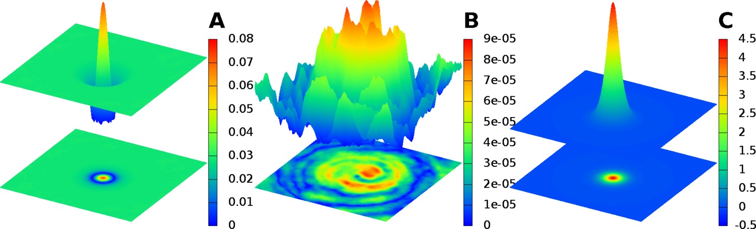
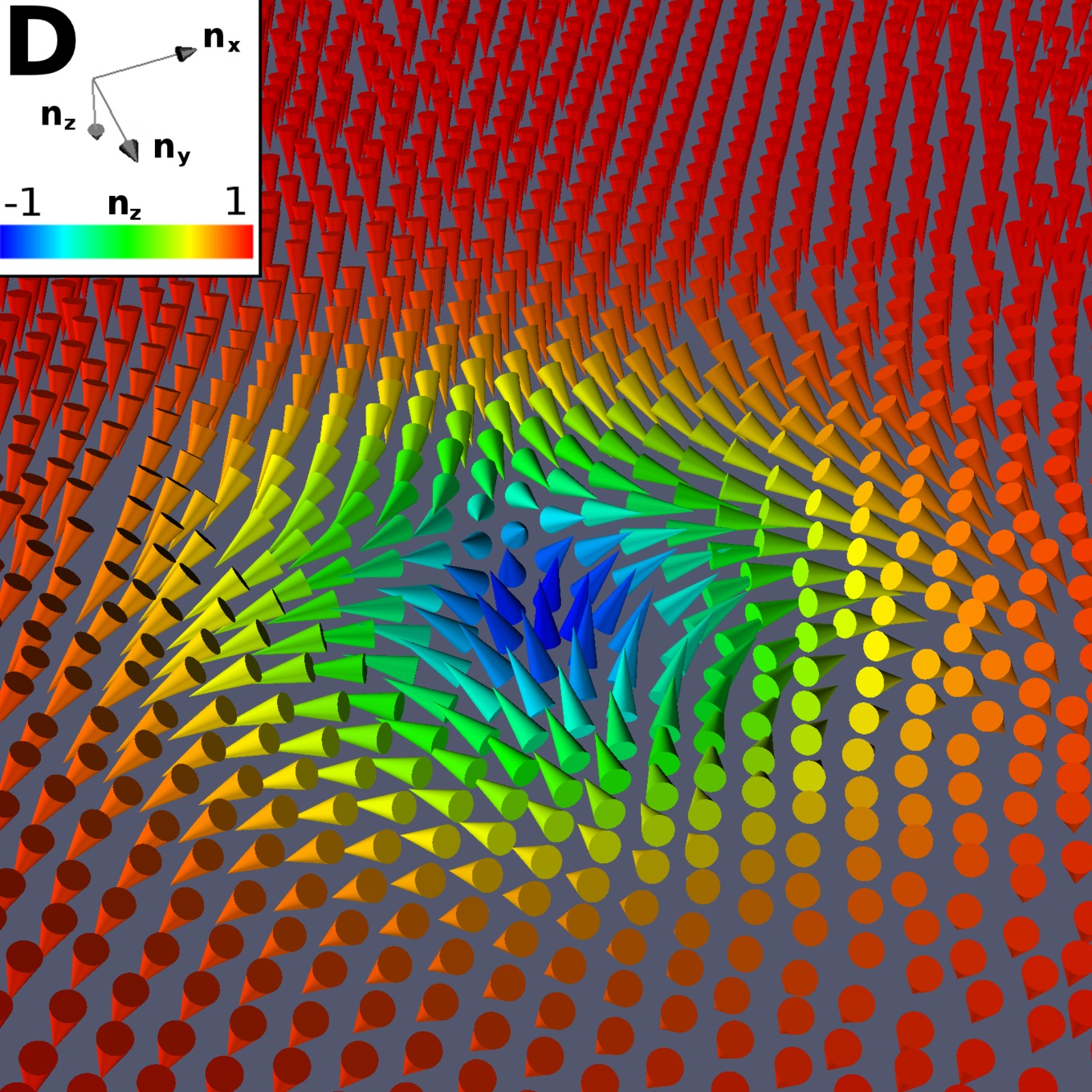
Figure 16: (Color online) – The $\mathcal{Q}=1$ soliton for the $U(3)$ symmetric model broken by Josephson interactions of the form (5.42), with $\Lambda=20$ and $\eta_{0}=1$. The quantities $|1-|\psi|^{2}|$ (panel $\bf A$), and $|e_{3}^{\dagger}\Psi|$ (panel $\bf B$), measure the deviation from the $\sigma$-model. They converge to zero as $\Lambda$ is increased. Panel $\bf C$ shows the energy density of the skyrmion.The fourth panel (panel $\bf D$) displays the texture of the field ${\bf n}$, which is similar to that of a baby skyrmion.

V.4 The sigma model limit

In this section we consider the $k$-component GL model with potential

$$V=\frac{1}{2}\Lambda(1-|\Psi|^{2})^{2}-\frac{1}{2}\Psi^{\dagger}\eta\Psi$$ (5.36)

in the limit $\Lambda\rightarrow\infty$, where $\eta$ is a real-symmetric $k\times k$ matrix, with zero diagonal, parametrizing a general collection of Josephson interactions. In the notation of Sec. II this is the case $-\alpha_{a}=\beta_{a}=\gamma_{ab}=\Lambda$ for all $a,b$. The special case where $\eta=0$, $\Lambda\rightarrow\infty$ and $e\rightarrow\infty$, which reduces to a pure sigma model, was considered in Refs. golo, ; dadda, . It is possible to find explicit formulae for the topological solitons in that case. The case of finite $\Lambda$ and $e$, with $\eta=0$, has also been treated previously achucarro1 ; Hindmarsh:92 ; Achucarro.Vachaspati:00 . The field equations for the model (V.1) in the sigma model limit (in fact, in the case where $\Phi$ is valued in any compact kähler manifold) were studied in detail, from a geometric viewpoint, in Ref. spe, . Our focus here is on the new phenomena introduced by the Josephson terms $\eta$.

In terms of the polar coordinates $\rho,Z$, the limit $\Lambda\rightarrow\infty$ amounts to the constraint $\rho\equiv 1$, and the potential $V$ reduces, in this limit, to

$$V([Z])=-\frac{1}{2}Z^{\dagger}\eta Z=-\frac{1}{2}\frac{Z^{\dagger}\eta Z}{|Z|^{2}}.$$ (5.37)

We have included the factor of $|Z|^{2}$ in the denominator of this expression (which, of course, equals $1$ since $|Z|=1$ by definition) so that the right hand side is manifestly a function of the projective equivalence class of $Z$ only, not $Z$ per se, that is, $V([cZ])=V([Z])$ for all $c\in{\mathbb{C}}\backslash\{0\}$. This is convenient when one comes to compute the Hessian of $V$. Since $\eta$ is real symmetric, it has a unitary basis of eigenvectors $e_{1},e_{2},\ldots,e_{k}$, with corresponding real eigenvalues $\lambda_{1}\geq\lambda_{2}\geq\cdots\geq\lambda_{k}$. Expanding $Z$ relative to this basis

$$Z=\sum_{i=1}^{k}\chi_{i}e_{i},\qquad\chi\in{\mathbb{C}}^{k},\quad|\chi|=1,$$ (5.38)

we see that

$$V=-\frac{1}{2}\sum_{i=1}^{k}\lambda_{i}|\chi_{i}|^{2}.$$ (5.39)

Hence, the $U(k)$ symmetry of the model, which is preserved by the sigma-model limit, is broken by $\eta$ generically to $U(1)^{k}$. In the case where the spectrum of $\eta$ is degenerate, the breaking may be partial. For example, if $\lambda_{1}=\lambda_{2}$ and all other $\lambda_{i}$ are distinct, the free energy remains invariant under $U(2)\times U(1)^{k-1}$, where $U(2)$ acts in the obvious way on the span of $\{e_{1},e_{2}\}$.

Clearly, $V:{\mathbb{C}}{{P}}^{k-1}\rightarrow{\mathbb{R}}$ attains its minimum at $[Z]=[e_{1}]$, and this minimum is unique if $\lambda_{1}\neq\lambda_{2}$. If $\lambda_{1}=\lambda_{2}=\cdots=\lambda_{j}>\lambda_{j+1}\geq\cdots\geq\lambda_{k}$, then any $Z$ in the span of $\{e_{1},\ldots,e_{j}\}$ minimizes $V$, so the set of minima of $V$ is a ${\mathbb{C}}{{P}}^{j-1}$ submanifold of ${\mathbb{C}}{{P}}^{k-1}$. In this case, there can be no energy minimizer on ${\mathbb{R}}^{2}$ with $\mathcal{Q}\neq 0$, by Derrick’s scaling argument der , (i.e. solitons are unstable against expanding indefinitely) so let us assume, henceforth, that $\lambda_{1}\neq\lambda_{2}$, so that the vacuum of the model, $[e_{1}]$, is unique. If the field $\Phi=\pi\circ\Psi:{\mathbb{R}}^{2}\rightarrow{\mathbb{C}}{{P}}^{k-1}$ has topological charge $\mathcal{Q}=1$ then it wraps ${\mathbb{R}}^{2}$ once around some submanifold homologous to ${\mathbb{C}}{{P}}^{1}$ in ${\mathbb{C}}{{P}}^{k-1}$. In order to minimize the contribution of $V$, it should be the ${\mathbb{C}}{{P}}^{1}$ on which $\Psi$ lies in the span of $\{e_{1},e_{2}\}$, the sum of the two highest eigenspaces of $\eta$. So we predict that

$$\Psi\approx\chi_{1}e_{1}+\chi_{2}e_{2}$$ (5.40)

everywhere, where $\chi_{i}=e_{i}^{\dagger}\Psi$ are complex valued functions on ${\mathbb{R}}^{2}$. From the pair $(\chi_{1},\chi_{2})$ we can construct a $S^{2}$-valued field using the usual identification of ${\mathbb{C}}{{P}}^{1}$ with $S^{2}$, that is

$${\bf n}=(\overline{\chi}_{1}\>\>\overline{\chi}_{2})\mbox{\boldmath$\tau$}\left(\begin{array}[]{c}\chi_{1}\\ \chi_{2}\end{array}\right)$$ (5.41)

where $\mbox{\boldmath$\tau$}=(\tau_{1},\tau_{2},\tau_{3})$ are the Pauli spin matrices. In this way, a $\mathcal{Q}=1$ energy minimizer can, conjecturally, be identified with a degree 1 texture ${\bf n}:{\mathbb{R}}^{2}\rightarrow S^{2}$. Since $\Psi$ is parallel to $e_{1}$ at $|x|=\infty$, we see that $\chi_{2}(\infty)=0$, and hence ${\bf n}(\infty)=(0,0,1)^{T}$.

We present numerical evidence in favor of this conjecture in Fig. 16, in the case $k=3$,

$$\eta=\eta_{0}\left(\begin{array}[]{ccc}0&-1&-1\\ -1&0&-2\\ -1&-2&0\end{array}\right)$$ (5.42)

$\eta_{0}=1$ and $\Lambda=20$. It is found that $\Psi$ approximately satisfies the sigma-model constraint, more precisely, ${\varepsilon}_{1}=\max_{x\in{\mathbb{R}}^{2}}|1-|\Psi|^{2}|<0.04$. For this choice of $\eta$,

$$\lambda_{1}=2\eta_{0}\,,e_{1} =\frac{1}{\sqrt{2}}\left(\begin{array}[]{c}0\\ 1\\ -1\end{array}\right)$$ (5.46)

$$\lambda_{2}=(\sqrt{3}-1)\eta_{0}\,,e_{2} =\frac{1}{\sqrt{6+2\sqrt{3}}}\left(\begin{array}[]{c}\sqrt{3}+1\\ -1\\ -1\end{array}\right)$$ (5.50)

$$\lambda_{3}=-(\sqrt{3}+1)\eta_{0}\,,e_{3} =\frac{1}{\sqrt{6-2\sqrt{3}}}\left(\begin{array}[]{c}\sqrt{3}-1\\ 1\\ 1\end{array}\right).$$ (5.54)

We expect the $\mathcal{Q}=1$ energy minimizer to have $\Psi$ in the span of $\{e_{1},e_{2}\}$ which, since the eigenvectors form a unitary frame, is equivalent to satisfying $e_{3}^{\dagger}\Psi=0$. Again, this turns out to be approximately true: ${\varepsilon}_{2}=\max_{x\in{\mathbb{R}}^{2}}|e_{3}^{\dagger}\Psi|<0.03$. We find that both the errors ${\varepsilon}_{1}$ and ${\varepsilon}_{2}$ become smaller as $\Lambda$ increases with $\eta_{0}$ held fixed. This indicates that the sigma model limit is well founded and should be a reliable approximation for $\Lambda$ large but finite. Qualitatively, in this special case of the 3-component model, the ${\bf n}$ field we find numerically is similar to the field of a so-called baby-skyrmion pieschzak .

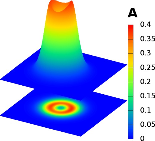
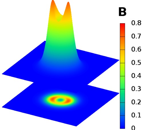
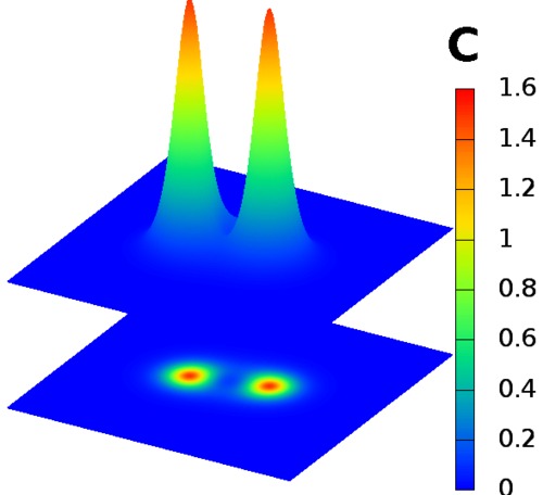
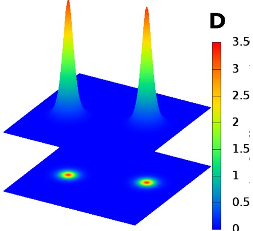
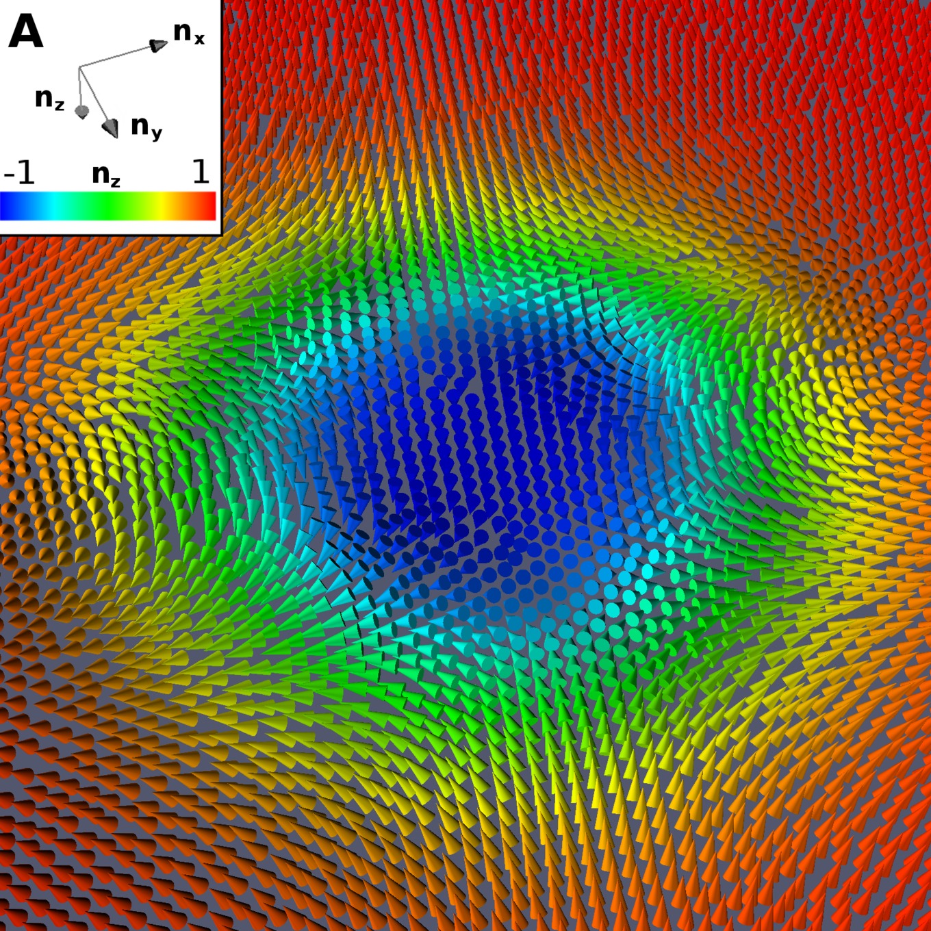
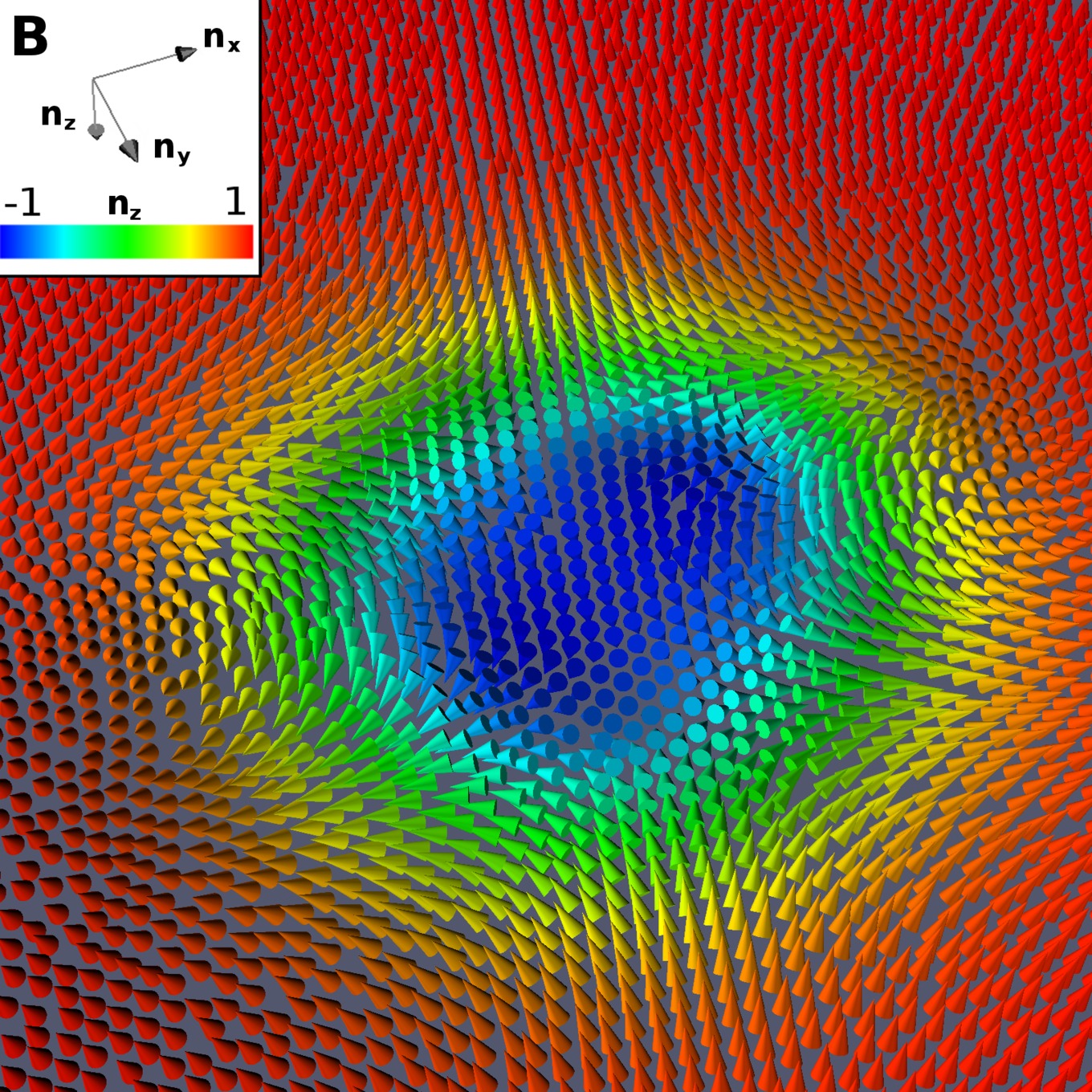
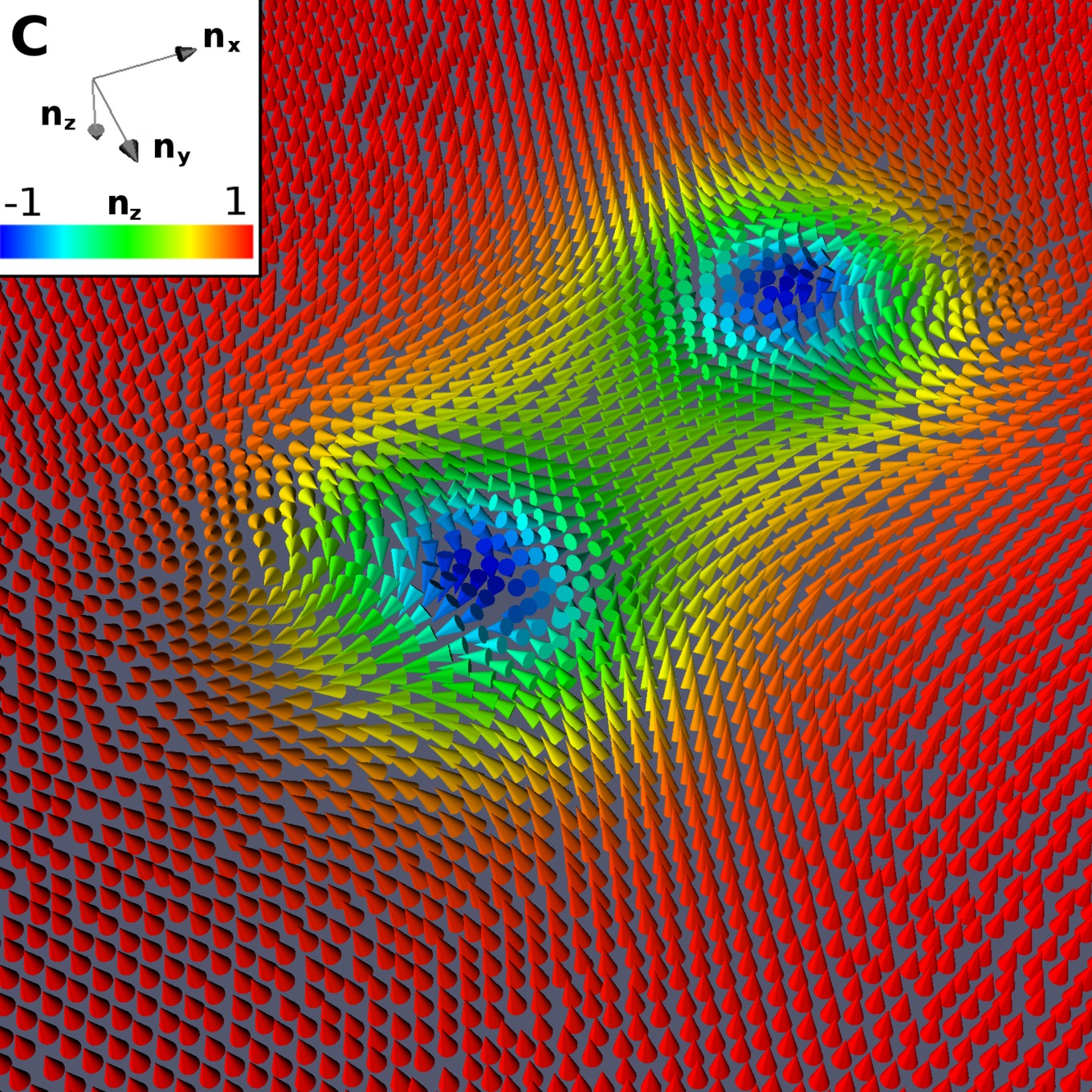
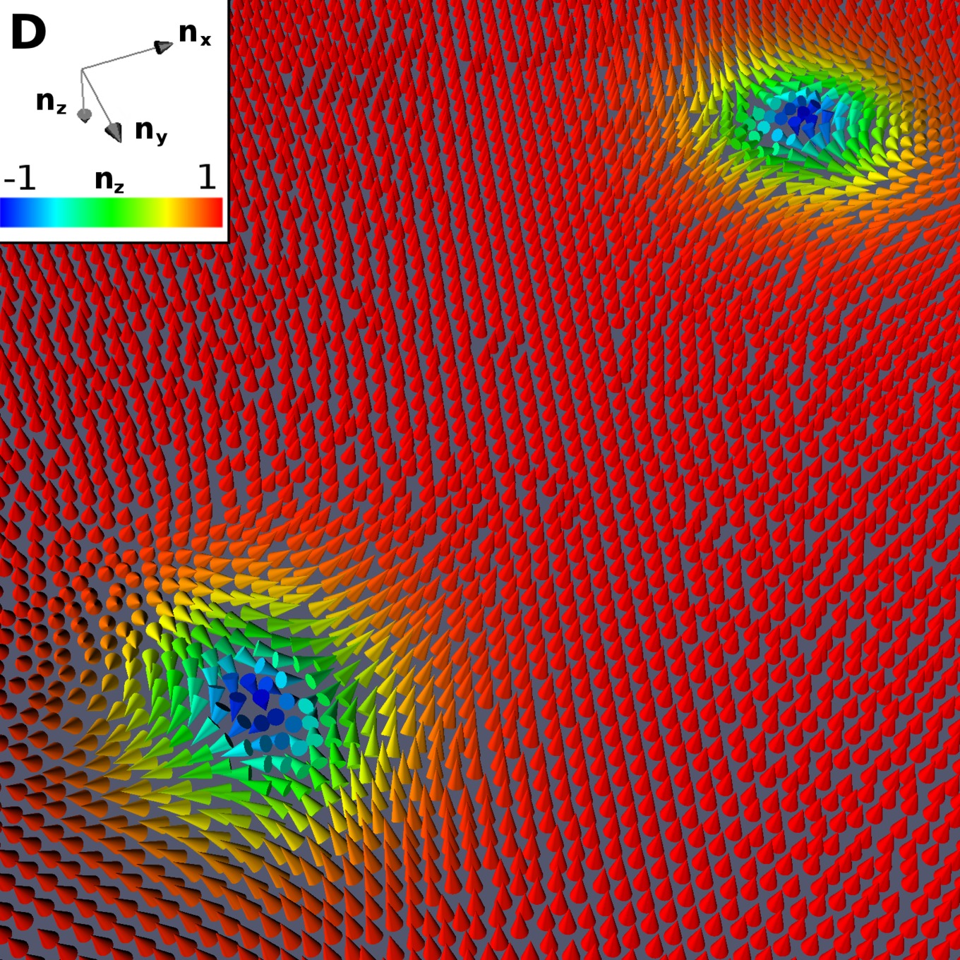
Figure 17: (Color online) – The results of energy minimization with charge $\mathcal{Q}=2$ for $\Lambda=20$, and $e=1.0$ and varying $\eta_{0}$. First row shows the energy density while the second and third row displays the corresponding texture field.Panels ($\bf A$, $\eta_{0}=0.1$), ($\bf B$, $\eta_{0}=0.2$)), ($\bf C$, $\eta_{0}=0.3$)), are for $\eta_{0}<\eta_{0}^{*}$ where interaction between skyrmions is attractive. Two $\mathcal{Q}=1$ skyrmions coalesce into either one $\mathcal{Q}=2$ skyrmion ($\bf A$, $\bf{B}$ and $\bf C$). Configuration displayed on panel $\bf{C}$ resemble bound state of two $\mathcal{Q}=1$ skyrmions. Panel ($\bf D$, $\eta_{0}=0.8$)) has $\eta_{0}>\eta_{0}^{*}$, then in the repulsive channel. Here the two $\mathcal{Q}=1$ skyrmions are repelling each other. So the snapshot on panel $\bf D$ shows a late but unconverged iteration (i.e. it represents a fairly converged pair of individual skyrmions which are, however, still drifting apart).

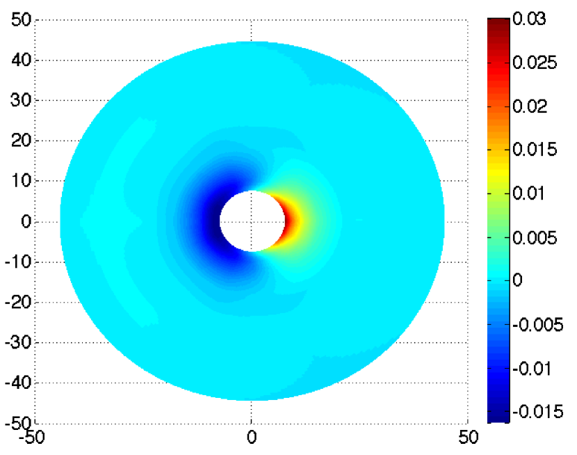
Figure 18: (Color online)– Interaction energy of two single quantum solitons. The the GL parameters are $\alpha_{a}=-20$, $\beta_{a}=20$, $\gamma_{ab}=20$, $\eta_{ab}=-1$ and $e=1$. Thus, the potential part of the free energy density can be written as $U=\lambda(1-|\psi_{1}|^{2}-|\psi_{2}|^{2}-|\psi_{3}|^{2})^{2}-\eta_{ab}|\psi_{a}||\psi_{b}|\cos(\varphi_{a}-\varphi_{b})$ with $\lambda=10$, i.e. the Hamiltonian features $SU(3)$ symmetry broken by Josephson interaction term.

If we place two $\mathcal{Q}=1$ energy minimizers a long distance apart and allow the system to relax, do they repel one another and escape to infinity, or do they attract one another and coalesce into a $\mathcal{Q}=2$ bound state? To predict this, we need to compute the spectrum of the Hessian of $V$ about $\Phi_{0}=[e_{1}]$, as described in Sec. V.3. In this case, $\rho$ is frozen by the constraint, so $P={\mathbb{C}}{{P}}^{k-1}$. It is useful to identify the tangent space $T_{[e_{1}]}{\mathbb{C}}{{P}}^{k-1}$ with the $(k-1)$-dimensional complex vector space

$${\mathbb{V}}=\{Y\in{\mathbb{C}}^{k}\>:\>e_{1}^{\dagger}Y=0\}.$$ (5.55)

Then the natural metric on $T_{p_{0}}P$ (5.31) reduces to

$$\langle Y,Y^{\prime}\rangle_{\mathbb{V}}=\mathrm{Re}(Y^{\dagger}Y^{\prime})$$ (5.56)

the restriction of the Euclidean metric on ${\mathbb{C}}^{k}$ to ${\mathbb{V}}$. To compute the Hessian of $V$ about $[e_{1}]$, we consider a curve $Z(t)$ in ${\mathbb{C}}^{k}$ with $Z(0)=e_{1}$ and $\dot{Z}(0)=Y\in{\mathbb{V}}$. Then

$${\sf Hess}_{[e_{1}]}(Y,Y) =\left.\frac{d^{2}\>}{dt^{2}}\right|_{t=0}V(\Psi(t))$$

$$=Y^{\dagger}[\lambda_{1}{\mathbb{I}}_{k}-\eta]Y$$

$$=\langle Y,(\lambda_{1}{\mathbb{I}}_{k}-\eta)Y\rangle_{{\mathbb{V}}}$$ (5.57)

where we have used the fact that $\lambda_{1}{\mathbb{I}}_{k}-\eta$ is self adjoint with $e_{1}$ in its kernel, so that $e_{1}^{\dagger}(\lambda{\mathbb{I}}_{k}-\eta)Y=0$. Hence, the associated self-adjoint linear map ${\cal H}_{[e_{1}]}:{\mathbb{V}}\rightarrow{\mathbb{V}}$ is the restriction to ${\mathbb{V}}$ of $\lambda_{1}{\mathbb{I}}_{k}-\eta$. It follows that the eigenvalues of ${\cal H}_{[e_{1}]}$ are $\lambda_{1}-\lambda_{i}$, $i=2,\ldots,k$, each of multiplicity $2$, and that the corresponding eigenspaces are two real-dimensional, spanned by $\{e_{i},ie_{i}\}$, $i=2,\ldots,k$. So there are $2k-2$ real scalar bosons in this model, occurring in pairs, having mass

$$m_{i}=\sqrt{\lambda_{1}-\lambda_{i}}.$$ (5.58)

This should be compared with the mass of the supercurrent field, i.e. the inverse London penetration length,

$$m_{J}=e.$$ (5.59)

Numerics suggest that the supercurrent of a $\mathcal{Q}=1$ energy minimizer is, at large $|x|$, similar to that of a vortex, while the lightest (complex) Klein-Gordon mode $\chi_{2}$ is similar to the asymptotic field of a baby-skyrmion. Hence, we expect $J$ to mediate a repulsive force of range $1/e$ and $\chi_{2}$ to mediate a short-range scalar dipole-dipole force. The range of this force is $1/\sqrt{\lambda_{1}-\lambda_{2}}$. The latter force is attractive provided the two solitons are appropriately aligned; see the discussion of baby-Skyrme models jayspesut for a detailed analysis. The dipole like interaction is also natural from the viewpoint of the fractional-vortex picture of skyrmions (see discussion in Sec. IV and in Refs. frac, ; smiseth, ). Hence, we predict that a pair of $\mathcal{Q}=1$ solitons, in the model which we consider in this subsection, always repel (for all relative orientations) if $e^{2}<\lambda_{1}-\lambda_{2}$, so higher $\mathcal{Q}$ bound states cannot form. On the other hand, if $e^{2}>\lambda_{1}-\lambda_{2}$, well-separated solitons have an attractive channel, and we predict that they can coalesce into higher $\mathcal{Q}$ bound states. Numerical evidence of this predicted dichotomy in the three component case is presented in Fig. 17 and direct numerical evidence of dipolar interaction of two $\mathcal{Q}=1$ skyrmions is presented in Fig. 18.

V.5 A symmetric case with BTRS

In this section we consider the GL⁽³⁾ model with three identical active bands, coupled through identical Josephson terms. The potential is

$$V(\Psi)=\frac{\lambda}{8}\sum_{a=1}^{3}(1-|\psi_{a}|^{2})^{2}+\frac{\eta}{2}\Psi^{\dagger}N\Psi,$$ (5.60)

where $N$ denotes the symmetric coupling matrix

$$N=\left(\begin{array}[]{ccc}0&1&1\\ 1&0&1\\ 1&1&0\end{array}\right).$$ (5.61)

Note that, in contrast to section V.4, $\eta$ denotes a real parameter here, not a matrix. In terms of the notation of section II, this is the special case $\alpha_{1}=\alpha_{2}=\alpha_{3}=-\frac{\lambda}{4}$, $\beta_{1}=\beta_{2}=\beta_{3}=\frac{\lambda}{4}$, $\gamma_{ab}=0$ and $\eta_{12}=\eta_{13}=\eta_{23}=-\eta$. The vacuum manifold for this potential is a disjoint union of two circles, the gauge orbits of

$$\Psi=\rho_{0}v_{0}\qquad\mbox{and}\qquad\Psi=\rho_{0}v_{1}$$ (5.62)

where

$$\rho_{0}=\sqrt{3+\frac{6\eta}{\lambda}},$$ (5.63)

and (with $\xi=e^{2\pi i/3}$)

$$v_{0}=\frac{1}{\sqrt{3}}\left(\begin{array}[]{c}1\\ \xi\\ \xi^{2}\end{array}\right),\leavevmode\nobreak\ v_{1}=\frac{1}{\sqrt{3}}\left(\begin{array}[]{c}1\\ \xi^{2}\\ \xi\end{array}\right),\leavevmode\nobreak\ v_{2}=\frac{1}{\sqrt{3}}\left(\begin{array}[]{c}1\\ 1\\ 1\end{array}\right),$$ (5.64)

are simultaneous unit eigenvectors of the symmetric coupling matrix $N$ and the permutation matrix $P$,

$$P=\left(\begin{array}[]{ccc}0&0&1\\ 1&0&0\\ 0&1&0\end{array}\right).$$ (5.65)

Note that

$$Nv_{0}=-v_{0},\quad Nv_{1}=-v_{1},\quad Nv_{2}=2v_{2},$$ (5.66)

$$Pv_{0}=\xi v_{0},\quad Pv_{1}=\xi^{2}v_{1},\quad Pv_{2}=v_{2}.$$ (5.67)

We shall, without loss of generality, choose the vacuum $\rho_{0}v_{0}$ (rather than $\rho_{0}v_{1}$). Since $[\overline{\Psi}]\neq[\Psi]$ for this vacuum, the model has broken time-reversal symmetry.

There are axially symmetric vortex solutions which interpolate between $(0,0,0)$ at $r=0$ and the above vacuum at $r=\infty$. To construct them, one only needs to solve a single component GL model:

$$F_{*}=\int_{{\mathbb{R}}^{2}}\Bigg{\{}\frac{1}{2}|\mathrm{d}A|^{2}+\frac{1}{2}|D\phi|^{2}+\frac{\lambda}{24}(\rho_{0}^{2}-|\phi|^{2})^{2}\Bigg{\}}.$$ (5.68)

Given a vortex solution $(\phi,A)$ of (5.68),

$$\Psi=\phi v_{0},\qquad A$$ (5.69)

is a vortex solution of the symmetric GL⁽³⁾ model (5.60). The numerical results of Sec. II strongly suggest that (5.60) also supports skyrmion solutions, at least for $\mathcal{Q}$ and $1/e$ sufficiently large.

Once again, we wish to compute the spectrum for the Hessian of $V$ about the vacuum $(\rho_{0},[v_{0}])$. The potential is, in polar coordinates (5.12),

$$V(\rho,Z) =\frac{\lambda}{8}\sum_{a=1}^{3}(1-\rho^{2}{|Z_{a}|^{2}})^{2}+\frac{\eta}{2}\rho^{2}{Z^{\dagger}NZ}$$ (5.70)

$$=\frac{3\lambda}{8}-\frac{\lambda}{4}\rho^{2}+\frac{\lambda}{8}\rho^{4}U([Z])+\frac{\eta}{2}\widetilde{U}([Z])$$ (5.71)

where

$$U([Z]) =\frac{1}{|Z|^{4}}\sum_{a=1}^{3}|Z_{a}|^{4}$$ (5.72)

$$\widetilde{U}([Z]) =\frac{Z^{\dagger}NZ}{|Z|^{2}}.$$ (5.73)

We have included the factors of $|Z|^{2}$ in the denominators of these expressions (which, of course, equals $1$ by definition) so that the right hand sides are manifestly functions $[Z]$ only. Recall that ${\sf Hess}$ is a symmetric bilinear form on the tangent space to $(0,\infty)\times{\mathbb{C}}{{P}}^{2}$ at the vacuum $(\rho_{0},[v_{0}])$. In general, there is no reason why this bilinear form should not couple the direction tangent to $(0,\infty)$ with directions tangent to ${\mathbb{C}}{{P}}^{2}$. We shall see that in this case permutation symmetry prevents such coupling.

First, we note that $[v_{0}]$ is a fixed point of the permutation map

$${\cal P}:{\mathbb{C}}{{P}}^{2}\rightarrow{\mathbb{C}}{{P}}^{2},\qquad[Z]\mapsto[PZ],$$ (5.74)

and that $\mathrm{d}{\cal P}_{[v_{0}]}:T_{[v_{0}]}{\mathbb{C}}{{P}}^{2}\rightarrow T_{[v_{0}]}{\mathbb{C}}{{P}}^{2}$ has maximal rank, so it follows that $[v_{0}]$ is a critical point of any function ${\mathbb{C}}{{P}}^{2}\rightarrow{\mathbb{R}}$ invariant under ${\cal P}$. In particular,

$$\mathrm{d}U_{[v_{0}]}=\mathrm{d}\widetilde{U}_{[v_{0}]}=0.$$ (5.75)

Consider now a two-parameter variation $p(s,t)=(\rho(s),[Z(t)])$ through $p_{0}=(\rho_{0},[v_{0}])$ in $P=(0,\infty)\times{\mathbb{C}}{{P}}^{2}$, with $\partial_{s}p(0,0)=(\sigma,0)$ and $\partial_{t}p(0,0)=(0,Y)$. Then

$${\sf Hess}_{p_{0}}((\sigma,0),(0,Y)) =\left.\frac{\partial^{2}V(p(s,t))}{\partial s\partial t}\right|_{s=t=0}$$

$$=\frac{\lambda}{4}\rho_{0}^{3}\sigma\mathrm{d}U_{[v_{0}]}Y+\eta\rho_{0}\sigma\mathrm{d}\widetilde{U}_{[v_{0}]}Y$$

$$=0$$ (5.76)

by (5.75). Hence

$${\sf Hess}=(\lambda+2\eta)\mathrm{d}\rho_{\rho_{0}}^{2}+\frac{\lambda}{8}\rho_{0}^{4}H+\frac{\eta}{2}\rho_{0}^{2}\widetilde{H}$$ (5.77)

where $H,\widetilde{H}:T_{[v_{0}]}{\mathbb{C}}{{P}}^{2}\times T_{[v_{0}]}{\mathbb{C}}{{P}}^{2}\rightarrow{\mathbb{R}}$ are the Hessians of the functions $U,\widetilde{U}$ respectively. It follows that one of the real scalar bosons $\alpha_{i}$ in (V.3) is just $\sigma$ (the linearization of $\rho$ about $\rho_{0}$) and that this has mass

$$m_{\rho}=\sqrt{\lambda+2\eta}.$$ (5.78)

It remains to compute $H$ and $\widetilde{H}$. For this purpose, we identify the tangent space $T_{[v_{0}]}{\mathbb{C}}{{P}}^{2}$ with the two dimensional complex vector space

$${\mathbb{V}}=\{Y\in{\mathbb{C}}^{3}\>:\>v_{0}^{\dagger}Y=0\}$$ (5.79)

which is spanned by $\{v_{1},v_{2}\}$, and give ${\mathbb{V}}$ the induced Euclidean metric

$$\langle X,Y\rangle_{\mathbb{V}}=\frac{1}{2}(X^{\dagger}Y+Y^{\dagger}X)=\frac{1}{4}\langle X,Y\rangle_{FS}$$ (5.80)

where $\langle\cdot,\cdot\rangle_{FS}$ denotes the Fubini-Study metric, used to compute $|\mathrm{d}Y|^{2}$ in equation (V.1).

In fact, we already know $\widetilde{H}$, since this is a special case of the general Josephson coupling matrix considered in section V.4:

$$\widetilde{H}(X,Y)=2\langle X,(N+1)Y\rangle_{{\mathbb{V}}}$$ (5.81)

It is convenient to expand $X,Y$ relative to the unitary (for $\langle\cdot,\cdot\rangle_{{\mathbb{V}}}$) basis $v_{1},v_{2}$, which are eigenvectors of $N$. Namely, if

$$X =(x_{1}+ix_{2})v_{1}+(x_{3}+ix_{4})v_{2},$$

$$Y =(y_{1}+iy_{2})v_{1}+(y_{3}+iy_{4})v_{2}$$ (5.82)

then

$$\widetilde{H}(X,Y)=6x^{T}\left(\begin{array}[]{cccc}0&0&0&0\\ 0&0&0&0\\ 0&0&1&0\\ 0&0&0&1\end{array}\right)y.$$ (5.83)

Note that this is a hermitian bilinear form on ${\mathbb{V}}$, that is $\widetilde{H}(iX,iY)=\widetilde{H}(X,Y)$.

Turning to $H$, one should not expect it to be hermitian, because $U$ contains terms like $Z_{1}^{2}\overline{Z}_{1}^{2}$. Consider a two-parameter variation $Z_{s,t}$ in $S^{5}\subset{\mathbb{C}}^{3}$ with $Z_{0,0}=v_{0}$ and $\partial_{s}Z_{s,t}|_{0,0}=X\in{\mathbb{V}}$, $\partial_{t}Z_{s,t}|_{0,0}={\mathbb{V}}$. By definition,

$$H(X,Y)=\left.\frac{\partial^{2}U(Z_{s,t})}{\partial s\partial t}\right|_{s=t=0}.$$ (5.84)

Using the explicit formula (5.72) for $U(Z)$, we find that

$$H(X,Y)=2\sum_{a=1}^{3}(\overline{X}_{a}Z_{a}+\overline{Z}_{a}X_{a})(\overline{Y}_{a}Z_{a}+\overline{Z}_{a}Y_{a})\leavevmode\nobreak\ \leavevmode\nobreak\$$ (5.85)

where $Z=v_{0}$. Note this is not Hermitian because, for example $H(iv_{1},iv_{2})=-H(v_{1},v_{2})$. Again, we can express this as a $4\times 4$ real matrix, by expanding $X,Y$ relative to $v_{1},v_{2}$. One finds that

$$H(X,Y)=\frac{4}{3}x^{T}\left(\begin{array}[]{cccc}1&0&1&0\\ 0&1&0&-1\\ 1&0&1&0\\ 0&-1&0&1\end{array}\right)y.$$ (5.86)

Substituting (5.86) and (5.83) into (5.77), then (5.77) into (V.3), we obtain

$$F_{lin} =\int_{M}\Bigg{\{}\frac{1}{2e^{4}\rho_{0}^{4}}(\|\mathrm{d}J\|^{2}+e^{2}\rho_{0}^{2}\|J\|^{2})$$

$$+\frac{1}{2}(|\mathrm{d}\sigma|^{2}+(\lambda+2\eta)\sigma^{2})+\frac{1}{2}\rho_{0}^{2}\left(|\mathrm{d}y|^{2}+y^{T}{\cal M}y\right)\Bigg{\}}$$ (5.87)

where the mass matrix is

$${\cal M}=\frac{\lambda\rho_{0}^{2}}{6}\left(\begin{array}[]{cccc}1&0&1&0\\ 0&1&0&-1\\ 1&0&1&0\\ 0&-1&0&1\end{array}\right)+3\eta\left(\begin{array}[]{cccc}0&0&0&0\\ 0&0&0&0\\ 0&0&1&0\\ 0&0&0&1\end{array}\right).$$ (5.88)

The squared masses of the bosons tangent to ${\mathbb{C}}{{P}}^{2}$ are the eigenvalues of this matrix, namely

$$m_{\pm}^{2}=\frac{\lambda\rho_{0}^{2}}{6}\left\{1+\frac{9\eta}{\lambda\rho_{0}^{2}}\pm\sqrt{1+\left(\frac{9\eta}{\lambda\rho_{0}^{2}}\right)^{2}}\right\},$$ (5.89)

each of multiplicity two. These should be compared with the mass of the $J$ vector boson and $\rho$ scalar boson

$$m_{J}^{2}=e^{2}\rho_{0}^{2},\qquad m_{\rho}^{2}=\lambda+2\eta.$$ (5.90)

To extract information about intersoliton forces, note that the embedded vortex (5.69) excites only the (repulsive) $J$ mode and the (attractive) $\rho$ mode, so one predicts the usual behaviour (i.e. for the example considered here where there is degeneracy in couplings between components, at long range vortices repel if $m_{\rho}>m_{J}$, and attract if $m_{\rho}<m_{J}$). Note that in the case when the components have different prefactors in $V$, there are also type-1.5 regimes with non-monotonic intervortex (long-range attractive, short-range repulsive) intervortex forces Carlstrom.Garaud.ea:11a . Skyrmions, on the other hand, should in all cases excite all 6 modes, with a monopole source for $\rho$ and dipole (or higher) sources for the 4 (mixed) $Y$ modes. So an interesting regime would be $m_{-}<m_{J}<m_{\rho}$ since then intervortex forces should be long-range repulsive, while inter-skyrmion forces should have an attractive channel for a certain relative orientations of skyrmions.

VI Conclusions

We discussed a new kind of topological soliton which we term chiral $GL^{(3)}$ skyrmions. These solitons occur in three-component superconductors when time reversal symmetry is spontaneously broken. In contrast to vortices, these skyrmions are characterized by a $\ {\mathbbm{C}}{{P}}^{2}\$topological charge. These skyrmions have a definite chirality associated with them: i.e. the order of the constituent fractional vortices matters, different orders giving inequivalent solutions. We described two situations

• A type-II BTRS superconductor can form a vortex lattice as a ground state in applied magnetic field. However in contrast to usual vortex states, all the regimes investigated by us possessed other flux-carrying topological defects of a higher energy: metastable $GL^{(3)}$ skyrmions characterized by a $\ {\mathbbm{C}}{{P}}^{2}\$topological charge. The system thus can form infinitely many complex metastable states in external fields where vortices coexist with the $GL^{(3)}$ skyrmions solitons. Thermal, or magnetic field quench can force the system to fall into one of these states.

• BTRS three-band superconductors in principle can have also a different regime where in external field $\ {\mathbbm{C}}{{P}}^{2}\$solitons are energetically cheaper than vortices. In that case the system cannot form vortices since they are unstable against decay into skyrmions. Such regimes occur for example when the free energy has bi-quadratic interaction terms of the form $\gamma_{ab}|\psi_{a}|^{2}|\psi_{b}|^{2}$.

In the regimes where chiral $GL^{(3)}$ skyrmions are metastable they can spontaneously form from ‘collisions’ of vortices, where intervortex interaction energy can be larger than energy of potential barrier of forming a skyrmion. We investigated several hundred regimes and found that skyrmions typically easily form in the energy minimization process where a system is relaxed from various higher energy states (such as dense groups of ordinary vortices). Our study indicates that the “capture basin” of these solutions can in certain cases be very large. We find that these defects very easily form during a rapid expansion of a vortex lattice (which should occur when magnetic field is rapidly lowered, or if a system is quenched through $H_{c2}$). Formation of solitons in this process can signal a state with Broken Time Reversal Symmetry. Also the potential barriers between Skyrmions and vortices or between different skyrmionic states can be overcome due to thermal fluctuations.

As shown in Fig. 1, these skyrmions have very particular magnetic signature and thus, under certain conditions, may be observed in high-resolution scanning SQUID, Hall, or magnetic force microscopy measurements. A tendency for vortex pair formation, yielding magnetic profile similar to that shown on Fig. 5 was observed in $\rm Ba(Fe_{1-x}Co_{x})_{2}As_{2}$, Kaliski as well as vortex clustering in $\rm BaFe_{2-x}Ni_{x}As_{2}$ Li . These materials have strong pinning which can naturally produce disordered vortex states Li , although the possibility of “type-1.5” scenario for these vortex inhomogeneities was also voiced in Ref. Li, . (Note that in three band (or higher number of bands) superconductors with frustrated Josephson coupling, type-1.5 regimes are easily obtainable even if Josephson coupling is very strong Carlstrom.Garaud.ea:11a .) The vortex pairs observed in Ref. Kaliski, can be discriminated from $\mathcal{Q}=2$ solitons by quenching the system in a stronger magnetic field and observing whether or not it forms vortex triangles, squares, pentagons, such as shown on e.g. Fig. 1 which correspond to flux profile of higher-$\mathcal{Q}$ solitons. Besides multiband superconductors, another class of systems which can support chiral $GL^{(3)}$ skyrmions is a Josephson coupled sandwich of an $s_{\pm}$ and $s$-wave superconductor.

The work is supported by the Swedish Research Council, by the Knut and Alice Wallenberg Foundation through the Royal Swedish Academy of Sciences fellowship and by NSF CAREER Award No. DMR-0955902, and by the UK Engineering and Physical Sciences Research Council. The computations were performed on resources provided by the Swedish National Infrastructure for Computing (SNIC) at National Supercomputer Center at Linkoping, Sweden.

Appendix A Fractional vortices have linearly divergent energy in the presence of Josephson coupling

Here we discuss fractional flux vortices in three band systems. Consider the case of one fractional vortex in which $\psi_{1}$ winds through $2\pi$ and neither $\psi_{2}$ nor $\psi_{3}$ winds. We assume that the configuration is spatially localized around $r=0$, so that on any annulus $\Omega=\{r_{0}<r<r_{1}\}$, with $r_{0}$ sufficiently large, the densities $|\psi_{a}|$ are close to their ground state values (i.e. we assume the London limit). It follows from expression (II) that the total free energy of any configuration satisfies the lower bound

$$F-F_{\mbox{\tiny GS}}\geq F_{\mbox{\tiny SG}}\,,$$ (A.91)

with $$F_{\mbox{\tiny SG}}:=\sum_{a<b}\nu_{ab}\int_{\Omega}|\nabla\varphi_{ab}|^{2}+\frac{1}{2}m_{ab}^{2}(1-\cos\varphi_{ab})$$

where $\nu_{ab}=|\psi_{a}|^{2}|\psi_{b}|^{2}/\rho^{2}$, $m_{ab}^{2}=2\eta_{ab}\rho^{2}/|\psi_{a}||\psi_{b}|$, and $\rho^{2}=\sum_{a}|\psi_{a}|^{2}$. $F_{\mbox{\tiny GS}}$ denotes the energy of the vortex-less ground state. In the London limit, the field densities assume their ground state values, so $\nu_{ab}$ and $m_{ab}$ are constants. In this limit, $F_{\mbox{\tiny SG}}$ simplifies to a sum of sine-Gordon energies (hence the subscript $SG$). Note that $|\nabla\varphi_{ab}|^{2}\geq r^{-2}(\partial\varphi_{ab}/\partial\theta)^{2}$, with $r$ and $\theta$, the polar coordinates around the vortex center. Hence,

$$F_{\mbox{\tiny SG}} \geq\sum_{a<b}\nu_{ab}\int_{\Omega}\left\{\frac{1}{r^{2}}\left(\frac{\partial\varphi_{ab}}{\partial\theta}\right)^{2}+m_{ab}^{2}\sin^{2}\frac{\phi_{ab}}{2}\right\}$$ (A.92)

$$=\sum_{a<b}\nu_{ab}\int_{\Omega}\left\{\left(\frac{1}{r}\frac{\partial\varphi_{ab}}{\partial\theta}-m_{ab}\sin\frac{\varphi_{ab}}{2}\right)^{2}\right.$$

$$\leavevmode\nobreak\ \leavevmode\nobreak\ \leavevmode\nobreak\ \leavevmode\nobreak\ \leavevmode\nobreak\ \leavevmode\nobreak\ \leavevmode\nobreak\ \leavevmode\nobreak\ \leavevmode\nobreak\ \leavevmode\nobreak\ \leavevmode\nobreak\ \leavevmode\nobreak\ \leavevmode\nobreak\ \leavevmode\nobreak\ \leavevmode\nobreak\ \leavevmode\nobreak\ \leavevmode\nobreak\ \leavevmode\nobreak\ \leavevmode\nobreak\ \leavevmode\nobreak\ \leavevmode\nobreak\ \leavevmode\nobreak\ \leavevmode\nobreak\ \leavevmode\nobreak\ \leavevmode\nobreak\ \leavevmode\nobreak\ \leavevmode\nobreak\ \leavevmode\nobreak\ \leavevmode\nobreak\ \leavevmode\nobreak\ \left.+\frac{2m_{ab}}{r}\frac{\partial\varphi_{ab}}{\partial\theta}\sin\frac{\varphi_{ab}}{2}\right\}$$ (A.93)

$$\geq\sum_{a<b}2m_{ab}\nu_{ab}\int_{r_{0}}^{r_{1}}dr\,r\int_{0}^{2\pi}\frac{1}{r}\frac{\partial\varphi_{ab}}{\partial\theta}\sin\frac{\varphi_{ab}}{2}$$ (A.94)

$$=8(m_{12}\nu_{12}+m_{13}\nu_{13})(r_{1}-r_{0})$$ (A.95)

where we have used the boundary conditions that $\varphi_{12}$ and $\varphi_{13}$ wind once, while $\varphi_{23}$ does not wind. So $F_{\mbox{\tiny SG}}$, and hence the total free energy $F-F_{\mbox{\tiny GS}}$, grows (at least) linearly with the system size, $r_{1}$.

Note that our lower bound on $F_{\mbox{\tiny SG}}$ cannot be attained, because for this to happen, one would need $\varphi_{ab}$ to satisfy

$$\frac{1}{r}\frac{\partial\varphi_{ab}}{\partial\theta}=m_{ab}\sin\frac{\varphi_{ab}}{2}$$ (A.96)

and no solutions to this PDE with the correct boundary behaviour ($\varphi_{12}(r,2\pi)-\varphi_{12}(r,0)=2\pi$ for all $r$) exist.

Appendix B Finite element energy minimization

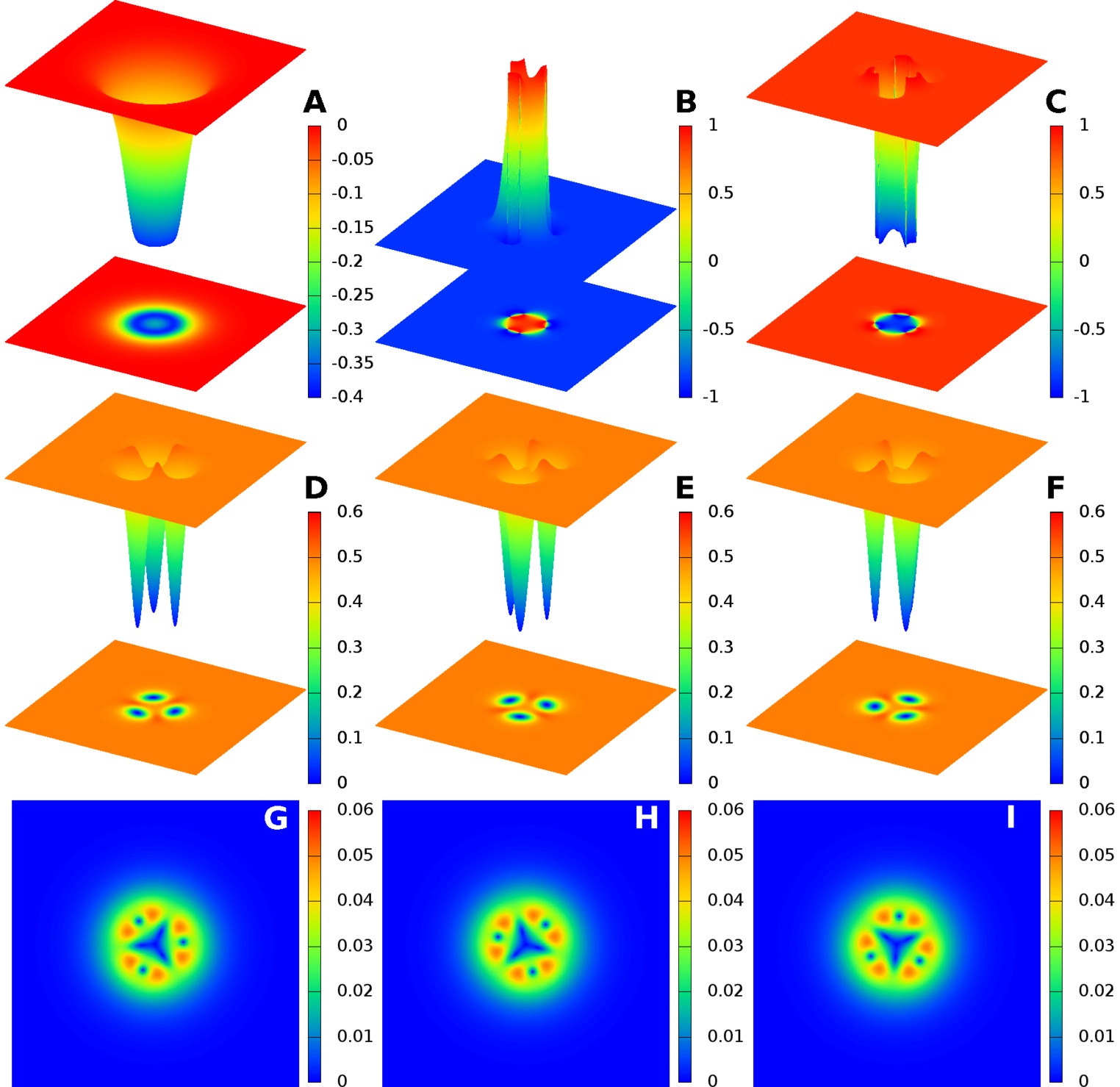
Figure 19: (Color online) – A $\mathcal{Q}=3$ quanta soliton in a system with three identical passive bands as in Fig. 3, except that there are no density-density interactions $\gamma_{ab}=0$ and $e=0.3$. Since the three bands are identical, the soliton makes a homogeneous ringlike configuration. Displayed quantities are the same as in rest of the paper.

The chiral skyrmions are either global or local minima of the Ginzburg-Landau energy (II). In the later case, this means that a good enough initial guess is necessary. In both cases, the functional minimization of (II), from an appropriate initial guess carrying several flux quanta, should lead to a chiral skyrmion (if it exists as a stable solution). We consider the two-dimensional problem (II) defined on the bounded domain $\Omega\subset\mathbbm{R}^{2}$ with $\partial\Omega$ its boundary. In practice we choose $\Omega$ to be a disk. Actually, the particular shape of the domain is not important. Indeed it is much larger than the typical size of solitons. Moreover, neither solitons nor initial guess coincide with some grid symmetry. For example, skyrmions are never placed at the center of the domain (the vizualization scheme re-centers the window around the soliton). This is an addtional argument that skyrmions are not boundary artefacts. One some occasions, we doubled checked on square domains that our solutions are unaffected by boundaries.

The problem is supplemented by the boundary condition $\boldsymbol{n}\cdot\boldsymbol{D}\Psi_{a}=0$ with $\boldsymbol{n}$ the normal vector to $\partial\Omega$. Physically this condition implies there is no current flowing through the boundary. Since this boundary condition is gauge invariant, additional constraint can be chosen on the boundary to fix the gauge. Our choice is to impose the radial gauge on the boundary $\boldsymbol{e}_{\rho}\cdot\boldsymbol{A}=0$ (note that with our choice of domain, this is equivalent to $\boldsymbol{n}\cdot\boldsymbol{A}=0$). With this choice, (most of) the gauge degrees of freedom are eliminated and the ‘no current flow’ condition separates in two parts

$$\boldsymbol{n}\cdot\nabla\psi_{a}=0\leavevmode\nobreak\ \leavevmode\nobreak\ \leavevmode\nobreak\ \leavevmode\nobreak\ \leavevmode\nobreak\ \leavevmode\nobreak\ \text{and}\leavevmode\nobreak\ \leavevmode\nobreak\ \leavevmode\nobreak\ \leavevmode\nobreak\ \leavevmode\nobreak\ \leavevmode\nobreak\ \boldsymbol{n}\cdot\boldsymbol{A}=0\,.$$ (B.97)

Note that these boundary conditions allow a topological defect to escape from the domain, since there is no pressure of an external applied field. Because they are topological defects, vortices (and skyrmions) cannot unwind. However, they can be ‘absorbed’ through the boundary in order to further minimize the energy. To prevent this, the numerical grid is chosen to be large enough so that the attractive interaction with the boundaries is negligible. The size of the domain is then much larger than the typical interaction length scales. Thus in this method one has to use large numerical grids, which is computationally demanding. The advantage is that it is guaranteed that obtained solutions are not boundary pressure artifacts.

The variational problem is defined for numerical computation using a finite element formulation provided by the Freefem++ library Hecht.Pironneau.ea . Discretization within finite element formulation is done via a (homogeneous) triangulation over $\Omega$, based on Delaunay-Voronoi algorithm. Functions are decomposed on a continuous piecewise quadratic basis on each triangle. The accuracy of such method is controlled through the number of triangles, (we typically used $3\sim 6\times 10^{4}$), the order of expansion of the basis on each triangle (2nd order polynomial basis on each triangle), and also the order of the quadrature formula for the integral on the triangles.

Once the problem is mathematically well defined, a numerical optimization algorithm is used to solve the variational nonlinear problem (i.e. to find the minima of $F$). We used here a nonlinear conjugate gradient method. The algorithm is iterated until relative variation of the norm of the gradient of the functional $F$ with respect to all degrees of freedom is less than $10^{-6}$.

Initial guess for obtaining metastable configurations

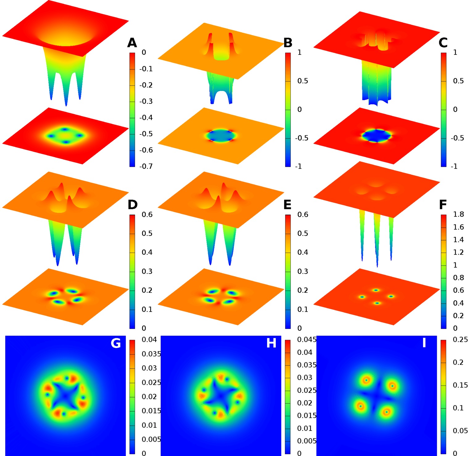
Figure 20: (Color online) – A $\mathcal{Q}=4$ quanta soliton in a system with two identical passive bands as in Fig. 5 coupled to a third active band with disparity in the ground state densities $(\alpha_{3},\beta_{3})=(-1.5,1)$. Josephson coupling constants are $\eta_{23}=-3$ and $\eta_{12}=\eta_{13}=1$. $e=0.2$ and $\gamma_{ab}=0$.

As discussed in the paper, $N$ quanta chiral skyrmions can be more energetically expensive than $N$ ordinary (type-II) vortices. In that case the initial guess should be within the attractive basin of the chiral skyrmions. Otherwise the configuration converges to ordinary type-II vortices which have the same total phase winding but cost less energy. The initial field configuration carrying $N$ flux quanta is prepared by using an ansatz which imposes phase windings around spatially separated $N$ vortex cores in each condensates.

$$\psi_{1} =|\psi_{1}|\mathrm{e}^{i\Theta_{1}}\,,\psi_{2}=|\psi_{2}|\mathrm{e}^{i\Theta_{2}+i\Delta_{2}}\,,\psi_{3}=|\psi_{3}|\mathrm{e}^{i\Theta_{3}+i\Delta_{3}}\,,\leavevmode\nobreak\ \leavevmode\nobreak\$$

$$|\psi_{a}| =u_{a}\prod_{k=1}^{N_{v}}\sqrt{\frac{1}{2}\left(1+\tanh\left(\frac{4}{\xi_{a}}({\cal R}^{a}_{k}(x,y)-\xi_{a})\right)\right)}\,,$$ (B.98)

where $a=1,2,3\,$ and $u_{a}\,$ is the ground state value of each condensate density. The parameters $\xi_{a}$ parametrize the core size while

$$\Theta_{a}(x,y) =\sum_{k=1}^{N}\tan^{-1}\left(\frac{y-y^{a}_{k}}{x-x^{a}_{k}}\right)\,,$$

$${\cal R}^{a}_{k}(x,y) =\sqrt{(x-x^{a}_{k})^{2}+(y-y^{a}_{k})^{2}}\,.$$ (B.99)

$(x^{a}_{k},y^{a}_{k})$ determines the position of the core of $k$-th vortex of the $a$-condensate.The functions $\Delta_{a}$ are used to seed a domain wall. As an initial guess we generally choose $\Delta_{2}=-\Delta_{3}\equiv\Delta$, with $\Delta$ defined as

$$\Delta=\frac{\pi}{3}\left(H({\mathbf{r}}-{\mathbf{r}}_{0})-1\right)\,,$$ (B.100)

where $H({\mathbf{r}}-{\mathbf{r}}_{0})$ is a Heaviside function. Thus in the initial guess the domain wall has infinitesimal thickness. It takes only a few steps from this initial guess to relax to a true domain wall during the simulations. Consequently, it is entirely sufficient to use Heaviside functions for the initial guesses for domain walls. The starting configuration of the vector potential is determined by solving Ampère’s law equation of (2.2) on the background of the superconducting condensates specified by (B)–(B.100). Being a linear equation in $\boldsymbol{A}$, this is an easy operation.

Once the initial configuration defined, all degrees of freedom are relaxed simultaneously, within the ‘no current flow’ boundary conditions discussed previously, to obtain highly accurate solutions of the Ginzburg-Landau equations. In a strongly type-II system when the initial guess was either (a) vortices placed on a closed domain wall or (b) closed domain wall surrounding a densely packed group of vortices, the system almost always formed chiral skyrmions. We used also initial guesses (c) without any domain walls ($\Delta=0$). In that case we observed chiral skyrmion formation, if in the initial states vortices were densely packed. This again indicates that the chiral skyrmions in the three component GL model represent (local) minima with wide capture basin in the free energy landscape.

Appendix C Additional Material

In this appendix we show few additional solutions Fig. 19, Fig. 20 and Fig. 21 for chiral skyrmions. Parameters sets, or number of flux quanta used here are different from the ones considered in the main body of the paper.

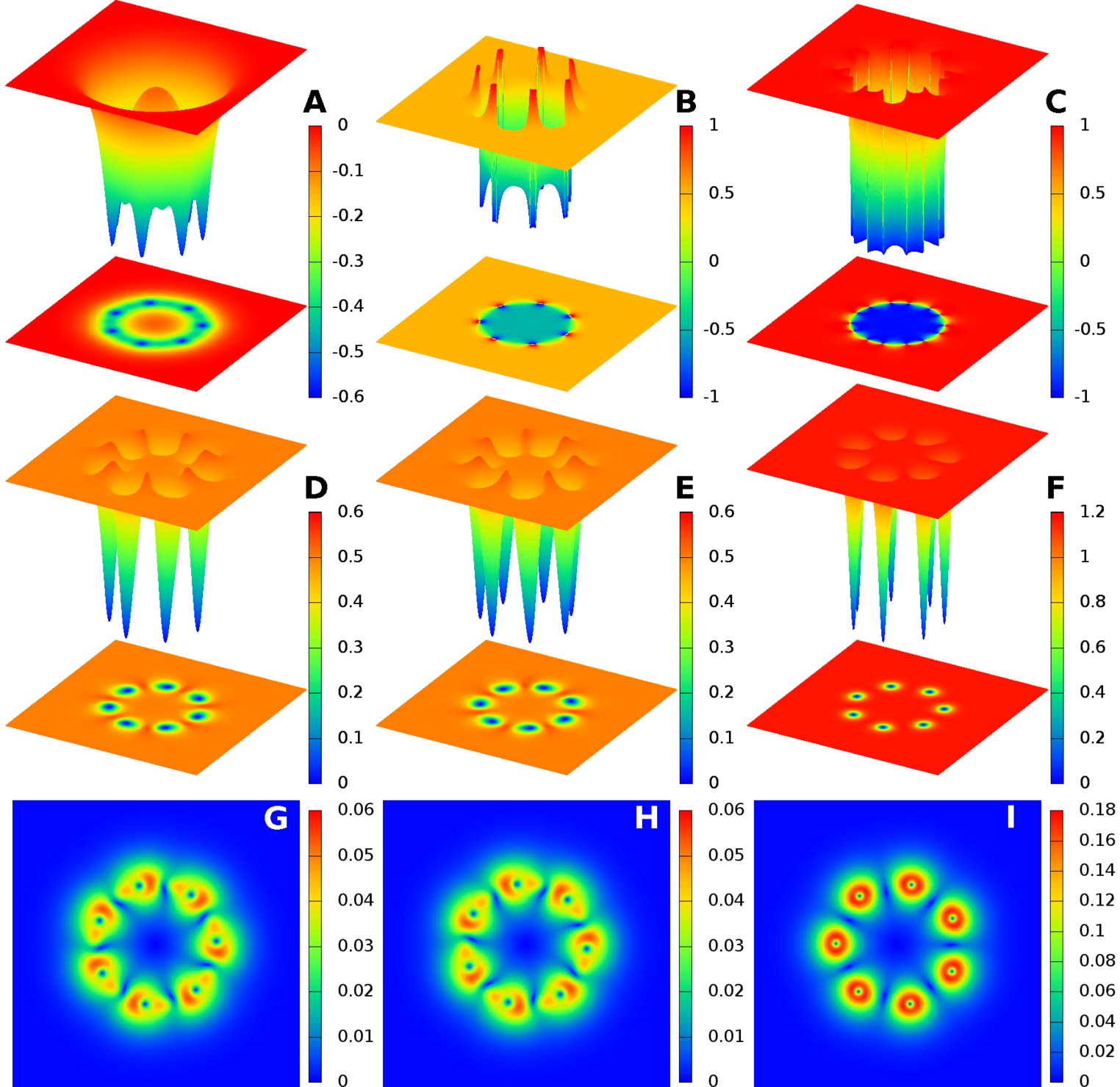
Figure 21: (Color online) – A $\mathcal{Q}=7$ quanta soliton in a system with two identical passive bands as in Fig. 5 coupled to a third active band with disparity in the ground state densities $(\alpha_{3},\beta_{3})=(-1,1)$. Josephson coupling constants are $\eta_{23}=-3$ and $\eta_{12}=\eta_{13}=1$. $e=0.3$ and $\gamma_{ab}=0$.

References

- (1) P.C.W. Chu, et al. (Eds.), Physica C 469, 313 (2009)
- (2) T. K. Ng and N. Nagaosa, Europhys. Lett. 87, 17003 (2009)
- (3) V. Stanev and Z. Tešanović, Phys. Rev. B 81, 134522 (2010)
- (4) W.-C. Lee, S.-C. Zhang, and C. Wu, Phys. Rev. Lett. 102, 217002 (2009)
- (5) C. Platt, R. Thomale, C. Honerkamp, S.-C. Zhang, and W. Hanke, Phys. Rev. B 85, 180502 (May 2012)
- (6) J. Garaud, J. Carlström, and E. Babaev, Phys. Rev. Lett. 107, 197001 (2011)
- (7) J. Carlström, J. Garaud, and E. Babaev, Phys. Rev. B 84, 134518 (Oct. 2011)
- (8) S. Mukherjee and D. F. Agterberg, Phys. Rev. B 84, 134520 (Oct. 2011)
- (9) X. Hu and Z. Wang, Phys. Rev. B 85, 064516 (Feb. 2012)
- (10) V. Stanev, Phys. Rev. B 85, 174520 (May 2012)
- (11) Y. Ota, M. Machida, T. Koyama, and H. Aoki, Phys. Rev. B 83, 060507 (2011)
- (12) V. Vakaryuk, V. Stanev, W.-C. Lee, and A. Levchenko, Phys. Rev. Lett. 109, 227003 (Nov 2012)
- (13) M. Nitta, M. Eto, T. Fujimori, and K. Ohashi, Journal of the Physical Society of Japan 81, 084711 (2012)
- (14) S.-Z. Lin, Phys. Rev. B 86, 014510 (Jul. 2012)
- (15) S.-Z. Lin and X. Hu, Phys. Rev. Lett. 108, 177005 (Apr. 2012)
- (16) E. Babaev and J. M. Speight, Phys. Rev. B 72, 180502 (2005)
- (17) M. Silaev and E. Babaev, Phys. Rev. B 85, 134514 (Apr. 2012)
- (18) E. Babaev, Phys. Rev. Lett. 89, 067001 (2002)
- (19) J. Smiseth, E. Smørgrav, E. Babaev, and A. Sudbø, Phys. Rev. B 71, 214509 (2005)
- (20) M. A. Silaev, Phys. Rev. B 83, 144519 (Apr. 2011)
- (21) E. Babaev, J. Jäykkä, and M. Speight, Phys. Rev. Lett. 103, 237002 (Dec. 2009)
- (22) S. Kobayashi and K. Nomizu, Foundations of Differential Geometry: Vol.: 2 (Interscience Publishers, 1969)
- (23) E. Babaev, L. D. Faddeev, and A. J. Niemi, Phys. Rev. B65, 100512 (2002)
- (24) M. Hindmarsh, Nucl. Phys. B 392, 461 (1993)
- (25) J. M. Speight, Phys. Rev. D55, 3830 (1997)
- (26) V. Golo and A. Perelomov, Phys. Lett. B 79, 112 (1978)
- (27) A. D’Adda, M. Lüscher, and P. D. Vecchia, Nucl. Phys. B 146, 63 (1978)
- (28) T. Vachaspati and A. Achúcarro, Phys. Rev. D 44, 3067 (Nov. 1991)
- (29) M. Hindmarsh, Phys. Rev. Lett. 68, 1263 (1992)
- (30) A. Achucarro and T. Vachaspati, Phys. Rept. 327, 347 (2000)
- (31) J. M. Speight, J. Geom. Phys. 60, 599 (2010)
- (32) G. H. Derrick, J. Math. Phys. 5, 1252 (1964)
- (33) B. M. A. G. Piette, B. J. Schroers, and W. J. Zakrzewski, Z. Phys. C 65, 165 (1995)
- (34) J. Jäykkä, M. Speight, and P. Sutcliffe, Proc. Roy. Soc. Lond. A 468, 1085 (2012)
- (35) B. Kalisky, J. R. Kirtley, J. G. Analytis, J.-H. Chu, I. R. Fisher, and K. A. Moler, Phys. Rev. B 83, 064511 (2011)
- (36) L. J. Li, T. Nishio, Z. A. Xu, and V. V. Moshchalkov, Phys. Rev. B 83, 224522 (2011)
- (37) F. Hecht, O. Pironneau, A. Le Hyaric, and K. Ohtsuka, The Freefem++ manual (2007) www.freefem.org