Theoretical Overview on the Flavor Issues of Massive Neutrinos

Abstract

We present an overview on some basic properties of massive neutrinos and focus on their flavor issues, including the mass spectrum, flavor mixing pattern and CP violation. The lepton flavor structures are explored by taking account of the observed value of the smallest neutrino mixing angle $\theta_{13}$. The impact of $\theta_{13}$ on the running behaviors of other flavor mixing parameters is discussed in some detail. The seesaw-induced enhancement of the electromagnetic dipole moments for three Majorana neutrinos is also discussed in a TeV seesaw scenario.

PACS numbers: 11.25.Hf, 123.1K

1 INTRODUCTION

It is well known that two important experimental results were in the news in 2012:

• On 8 March 2012, the Daya Bay Collaboration announced a $5.2\sigma$ discovery of $\theta_{13}\neq 0$ for this smallest neutrino mixing angle [1],

  $$\sin^{2}2\theta_{13}=0.092\pm 0.016({\rm stat})\pm 0.005({\rm syst})~{}~{}~{}~{}(\pm 1\sigma~{}{\rm range})\;,$$ (1)

  which is equivalent to $\theta_{13}\simeq 8.8^{\circ}\pm 0.8^{\circ}$. The convincing Daya Bay result puts the preliminary results of T2K [2], MINOS [3] and Double Chooz [4], which all hinted at $\theta_{13}\neq 0$ in 2011, on solid ground. In particular, the fact that $\theta_{13}$ is not strongly suppressed is a good news to the experimental attempts towards a measurement of CP violation in the lepton sector.

• On 4 July 2012, the ATLAS [5] and CMS [6] Collaborations at the Large Hadron Collider (LHC) independently announced the discovery of a Higgs-like boson at the mass scale of 125 GeV to 127 GeV. If this result turns out to be true, it will have an important impact on the development of neutrino physics because most of the neutrino mass models depend on the existence of the Higgs particle(s) and Yukawa interactions.

Therefore, a brief overview of where we are standing and where we are expecting to go makes sense.

The remaining parts of this review paper are organized as follows. In section 2 we give a fast overview of some fundamental neutrino properties, such as the speed of neutrinos, the nature of massive neutrinos and the number of neutrino species. Section 3 is devoted to a brief description of the flavor issues of charged leptons and neutrinos, including the mass spectrum, flavor mixing pattern and CP violation. We compare the observed pattern of quark flavor mixing with that of lepton flavor mixing. In section 4 we go into details of possible lepton flavor structures by outlining two phenomenological strategies and taking a number of typical examples. The impact of large $\theta_{13}$ on the running behaviors of other flavor mixing parameters is discussed in section 5 by using the one-loop renormalization-group equations (RGEs) in the framework of the minimal supersymmetric standard model (MSSM). Section 6 is devoted to the seesaw-enhanced electromagnetic dipole moments of three Majorana neutrinos based on a TeV seesaw scenario. A summary and some concluding remarks are given in section 7.

2 IMMEDIATE QUESTIONS ON NEUTRINOS

2.1 Really Superluminal?

The constancy of the speed of light $c$ in vacuum and the independence of physical laws from the choice of inertial systems are two fundamental propositions of the special relativity (SR) [7]. If our world is Lorentz invariant, a free particle’s energy $E$, momentum ${\bm p}$ and rest mass $m$ satisfy the relationship $\sqrt{E^{2}-|{\bm p}|^{2}c^{2}}=mc^{2}$. The velocity of this particle turns out to be $v=c\sqrt{1-m^{2}c^{4}/E^{2}}$, implying that it cannot travel faster than light in vacuum. Could a particle be superluminal? The answer would be yes if the particle had an imaginary mass (called a “tachyon” [8]) or if the Lorentz invariance were broken.

The OPERA Collaboration claimed a “convincing” measurement of the superluminal neutrinos in September 2011 [9]. But five months later this story ended up with a mistake of the bad connection of the optical fiber. The OPERA paper was updated in July 2012 by including the new sources of errors, and the new result was in agreement with the SR. Here let us quote Steven Weinberg’s comments on the original result of the OPERA experiment: “The report of this experiment is pretty impressive, but it bothers me that there is plenty of evidence that all sorts of other particles never travel faster than light, while observations of neutrinos are exceptionally difficult. It is as if someone said that there are fairies in the bottom of their garden, but they can only be seen on dark, foggy nights.”

An early measurement of the neutrino speed was done by using the pulsed pion beams (produced by the pulsed proton beams hitting a target) at the Fermilab in the 1970s [10, 11]. In this experiment the speed of muons was compared with that of neutrinos and antineutrinos. The same measurement was repeated in 2007 by using the MINOS detector [12]. In 2011 the speed of neutrinos was also measured in a few other long-baseline neutrino experiments, such as the ICARUS [13, 14], Borexino [15] and LVD [16] experiments. But the most stringent constraint on the speed of neutrinos was from the observational data of the Supernova 1987A [17, 18, 19]: $|v-c|/c\lesssim 10^{-9}$ obtained by comparing the arrival time of light with that of neutrinos.

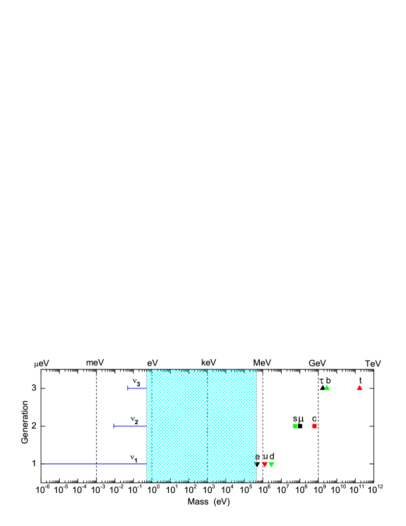
Figure 1: A schematic illustration of the “flavor hierarchy” and “flavor desert” problems in the fermion mass spectrum at the electroweak scale. Here the masses of three neutrinos are assumed to have a normal hierarchy.

2.2 Definitely Massive?

The neutrinos are massless in the standard model (SM) as a result of its simple structure and renormalizability. On the one hand, the SM does not contain any right-handed neutrinos, and thus there is no way to write out the Dirac neutrino mass term. On the other hand, the SM conserves the $SU(2)_{L}$ gauge symmetry and only contains the Higgs doublet, and thus the Majorana mass term is forbidden. Although the SM accidently possesses the $(B-L)$ symmetry and naturally allows neutrinos to be massless, the vanishing of neutrino masses in the SM is not guaranteed by any fundamental symmetry or conservation law. Today we have achieved a lot of robust evidence for neutrino oscillations from solar, atmospheric, reactor and accelerator neutrino experiments. The phenomenon of neutrino oscillations implies that at least two of the three neutrinos must be massive and the lepton flavors must be mixed. This is the first convincing evidence for new physics beyond the SM.

Fig. 1 is a schematic plot of the mass spectrum of the SM leptons and quarks at the electroweak scale. One can see that the span between $m_{1}$ and $m_{t}$ is at least twelve orders of magnitude. Furthermore, there exists an obvious “desert” spanning six orders of magnitude between the neutrino masses and the masses of the charged fermions. Why do the SM fermions have such hierarchy and desert puzzles? The answer to this important question remains open. In particular, the tiny neutrino masses must have a peculiar origin (e.g., via the seesaw mechanisms [20, 21, 22, 23, 24]). Moreover, there might exist one or more keV sterile neutrinos in the desert as a natural candidate for warm dark matter [25, 26, 27, 28, 29, 30, 31].

2.3 Dirac or Majorana?

A pure Dirac mass term added into the SM is in general disfavored, unless the theory is built by introducing extra dimensions. Such a mass term in a renormalizable model of electroweak interactions would worsen the fermion mass hierarchy problem. An effective Majorana mass term given by the right-handed neutrinos and their charge-conjugated counterparts is not forbidden by the SM gauge symmetry, unless the contrived assumption of lepton number conservation is imposed on the theory. Hence most theorists believe that massive neutrinos are more likely to be the Majorana particles and their salient feature is lepton number violation.

The unique window to verify the Majorana nature of massive neutrinos is to observe the neutrinoless doube-beta ($0\nu\beta\beta$) decay. So far we have not obtained very convincing evidence for this lepton-number-violating process. Even if the $0\nu\beta\beta$ decay were never observed, one would still be unable to conclude that massive neutrinos are the Dirac particles [32, 33]. The effective mass of the $0\nu\beta\beta$ decay could vanish if the Majorana CP-violating phases lie in some specific regions. On the other hand, there are some other mechanisms which can lead to the $0\nu\beta\beta$ decay. Such new physics effects could be of the same order as or even larger than the standard light-neutrino-exchange effect [34, 35].

Given the SM interactions, a massive Dirac neutrino can have a tiny (one-loop) magnetic dipole moment $\mu_{\nu}\sim 3\times 10^{-20}\mu_{\rm B}(m_{\nu}/0.1~{}{\rm eV})$, where $\mu_{\rm B}$ is the Bohr magneton [36, 37]. In contrast, a massive Majorana neutrino cannot have magnetic and electric dipole moments, because its antiparticle is just itself. Both Dirac and Majorana neutrinos can have transition dipole moments (of a size comparable with $\mu_{\nu}$) [38], which may give rise to neutrino decays, scattering effects with electrons, interactions with external magnetic fields (red-giant stars, the sun, supernovae, and so on), and contributions to neutrino masses. Current experimental bounds on the neutrino dipole moments are at the level of $\mu_{\nu}<{\rm a~{}few}\times 10^{-11}\mu_{\rm B}$.

2.4 More than Three Species?

It is well known that “three” is a mystically popular number in particle physics, such as three $Q=+2/3$ quarks, three $Q=-1/3$ quarks, three $Q=-1$ leptons, three $Q=0$ neutrinos, three colors and three forces in the SM. In this case, why do people want to go beyond $N_{\nu}=3$?

The study of light sterile neutrinos has become a popular direction in neutrino physics [39]. One is motivated to consider such “exotic” particles for several reasons. On the theoretical side, the type-I seesaw mechanism [20, 21, 22, 23, 24] provides a very elegant interpretation of the small masses of $\nu_{i}$ (for $i=1,2,3$) with the help of two or three heavy sterile neutrinos, and the latter can even help account for the observed matter-antimatter asymmetry of the Universe via the leptogenesis mechanism [40]. On the experimental side, the LSND [41], MiniBooNE [42] and reactor [43] antineutrino anomalies can all be explained as the active-sterile antineutrino oscillations in the assumption of one or two species of sterile antineutrinos whose masses are below 1 eV [44, 45]. Furthermore, a careful analysis of the existing data on the Big Bang nucleosynthesis [46] or the cosmic microwave background anisotropy, galaxy clustering and supernovae Ia [47, 48, 49] seems to favor at least one species of sterile neutrinos at the sub-eV mass scale. On the other hand, sufficiently long-lived sterile neutrinos in the keV mass range might serve for a good candidate for warm dark matter if they were present in the early Universe [50].

If the three known neutrinos have mixing with a few new degrees of freedom above or far above the Fermi scale, an exciting window will be open to new physics at high energy scales. In this case, however, the mixing between light and heavy neutrinos violates the unitarity of the $3\times 3$ light neutrino mixing matrix and might result in some observable effects in the future precision neutrino experiments [51].

3 NEUTRINO MASSES AND FLAVOR MIXING

There are three central concepts in flavor physics: mass, flavor mixing and CP violation [33]. The phenomenon of lepton flavor mixing at low energies is effectively described by a $3\times 3$ matrix $U$, the so-called Maki-Nakagawa-Sakata-Pontecorvo (MNSP) matrix [52, 53]. Given the unitarity of $U$, it can be parametrized in terms of three angles and three phases [54]:

$$U=\left(\begin{matrix}c_{12}c_{13}&s_{12}c_{13}&s_{13}e^{-i\delta}\cr-s_{12}c_{23}-c_{12}s_{13}s_{23}e^{i\delta}&c_{12}c_{23}-s_{12}s_{13}s_{23}e^{i\delta}&c_{13}s_{23}\cr s_{12}s_{23}-c_{12}s_{13}c_{23}e^{i\delta}&-c_{12}s_{23}-s_{12}s_{13}c_{23}e^{i\delta}&c_{13}c_{23}\cr\end{matrix}\right)P_{\nu}\;,$$ (2)

where $c_{ij}\equiv\cos\theta_{ij}$, $s_{ij}\equiv\sin\theta_{ij}$ (for $ij=12,13,23$), and $P_{\nu}={\rm Diag}\{e^{i\rho},e^{i\sigma},1\}$ is physically relevant if massive neutrinos are the Majorana particles.

Fogli et al [55] have recently done a global analysis of current neutrino oscillation data and obtained the ranges of two neutrino mass-squared differences ($\delta m^{2}\equiv m^{2}_{2}-m^{2}_{1}$ and $\Delta m^{2}\equiv|m^{2}_{3}-(m^{2}_{1}+m^{2}_{2})/2|$) and three neutrino mixing angles, as listed in Table 1, where NH and IH stand for the normal hierarchy ($m_{1}<m_{2}<m_{3}$) and the inverted hierarchy ($m_{3}<m_{1}<m_{2}$), respectively.

Results of the global $3\nu$ oscillation analysis by Fogli et al in 2012, including the best-fit values and allowed $1\sigma$, $2\sigma$ and $3\sigma$ ranges for the neutrino oscillation parameters. Parameter Best fit $1\sigma$ range $2\sigma$ range $3\sigma$ range $\delta m^{2}/10^{-5}~{}\mathrm{eV}^{2}$ (NH or IH) 7.54 7.32 – 7.80 7.15 – 8.00 6.99 – 8.18 $\sin^{2}\theta_{12}/10^{-1}$ (NH or IH) 3.07 2.91 – 3.25 2.75 – 3.42 2.59 – 3.59 $\Delta m^{2}/10^{-3}~{}\mathrm{eV}^{2}$ (NH) 2.43 2.33 – 2.49 2.27 – 2.55 2.19 – 2.62 $\Delta m^{2}/10^{-3}~{}\mathrm{eV}^{2}$ (IH) 2.42 2.31 – 2.49 2.26 – 2.53 2.17 – 2.61 $\sin^{2}\theta_{13}/10^{-2}$ (NH) 2.41 2.16 – 2.66 1.93 – 2.90 1.69 – 3.13 $\sin^{2}\theta_{13}/10^{-2}$ (IH) 2.44 2.19 – 2.67 1.94 – 2.91 1.71 – 3.15 $\sin^{2}\theta_{23}/10^{-1}$ (NH) 3.86 3.65 – 4.10 3.48 – 4.48 3.31 – 6.37 $\sin^{2}\theta_{23}/10^{-1}$ (IH) 3.92 3.70 – 4.31 3.53 – 4.84 $\oplus$ 5.43 – 6.41 3.35 – 6.63 $\delta/\pi$ (NH) 1.08 0.77 – 1.36 — — $\delta/\pi$ (IH) 1.09 0.83 – 1.47 — —

3.1 Neutrino Mass Spectrum

The two mass-squared differences of three neutrinos have been determined, to a very good degree of accuracy, from current experimental data: $\Delta m^{2}_{21}=\delta m^{2}\approx 7.5\times 10^{-5}~{}{\rm eV}^{2}$ and $\Delta m^{2}_{32}\approx\Delta m^{2}\approx\pm 2.4\times 10^{-3}~{}{\rm eV}^{2}$. The absolute neutrino mass scale remains unknown and may hopefully be determined in the following experimental or observational ways: the single $\beta$ decay, the $0\nu\beta\beta$ decay and the cosmological constraints. Fig. 2 shows the parameter space of $\Sigma\equiv m_{1}+m_{2}+m_{3}$, $m_{\beta}=\sqrt{m^{2}_{1}|U_{e1}|^{2}+m^{2}_{2}|U_{e2}|^{2}+m^{2}_{3}|U_{e3}|^{2}}$ (the effective electron neutrino mass in the $\beta$ decay) and $m_{\beta\beta}=|m_{1}U^{2}_{e1}+m_{2}U^{2}_{e2}+m_{3}U^{2}_{e3}|$ (the effective mass of the $0\nu\beta\beta$ decay). A precision measurement of $m_{\beta}$ and $\Sigma$ in the sub-eV range could determine the neutrino mass hierarchy. In the two lower panels of Fig. 2 there remains a large vertical spread in the allowed slanted bands, as a result of the unknown Majorana CP-violating phases in the $m_{\beta\beta}$ components. This observation indicates that more precise data in either the $(m_{\beta\beta},\,m_{\beta})$ plane or the $(m_{\beta\beta},\,\Sigma)$ plane might provide some useful constraints on the Majorana phases.

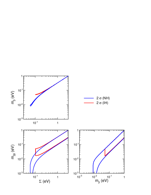
Figure 2: Constraints obtained by Fogli et al in 2012 (at the $2\sigma$ level) in the planes charted by any two among the absolute mass observables $m_{\beta}$ (the effective mass of the $\beta$ decay), $m_{\beta\beta}$ (the effective mass of the $0\nu\beta\beta$ decay) and $\Sigma$ (the sum of three neutrino masses). The blue (red) bands refer to the normal (inverted) neutrino mass hierarchy.

Before the absolute mass scale is determined, there remain two open questions: (1) is $m_{3}$ bigger or smaller than $m_{1}$? (2) can one neutrino mass ($m_{1}$ or $m_{3}$) be vanishing or vanishingly small? The first question awaits an experimental answer in the foreseeable future, such as a long-baseline neutrino oscillation experiment with appreciable terrestrial matter effects [56] or a long-baseline reactor antineutrino oscillation experiment with accurate information on the energy spectrum [57, 58]. A theoretical answer to the second question is strongly model-dependent. Examples of this type include the minimal type-I seesaw mechanism with two heavy Majorana neutrinos [59, 60] or the Friedberg-Lee ansatz with an effective Dirac or Majorana neutrino mass operator [61, 62, 63, 64, 65, 66, 67].

3.2 Flavor Mixing Pattern

The fact that the smallest neutrino mixing angle $\theta_{13}$ is not strongly suppressed leads us to some new questions about the feature of lepton flavor mixing: (1) Can the relatively large $\theta_{13}$ be understood by an underlying flavor symmetry or is it generated by a symmetry breaking mechanism or quantum corrections? (2) Does $\theta_{23}\simeq 45^{\circ}$ still hold? (3) What is the strength of leptonic CP violation?

The structure of the MNSP lepton flavor mixing matrix $U$ is significantly different from that of the Cabibbo-Kobayashi-Maskawa (CKM) quark flavor mixing matrix $V$. The CKM matrix is nearly the unit matrix up to some small corrections, while the MNSP matrix has an approximate $\mu$-$\tau$ symmetry. The full $\mu$-$\tau$ symmetry of $U$ in modulus is described by the equalities

$$|U_{\mu 1}|=|U_{\tau 1}|\;,~{}~{}~{}~{}|U_{\mu 2}|=|U_{\tau 2}|\;,~{}~{}~{}~{}|U_{\mu 3}|=|U_{\tau 3}|\;,$$ (3)

equivalent to two independent sets of conditions in the standard parametrization given in Eq. (2) [68]:

$$\theta_{23}=45^{\circ}\;,~{}~{}~{}\theta_{13}=0^{\circ}\;,$$ (4)

or

$$\theta_{23}=45^{\circ}\;,~{}~{}~{}\delta=\pm 90^{\circ}\;.$$ (5)

If $\theta_{23}$ is exactly equal to $45^{\circ}$, then one may arrive at a partial $\mu$-$\tau$ permutation symmetry in the MNSP matrix $U$ (i.e., the equality $|U_{\mu 3}|=|U_{\tau 3}|$).

Now that $\theta_{13}\neq 0^{\circ}$ has firmly been established by the Daya Bay experiment [1], it becomes crucial to check the deviation of $\theta_{23}$ from $45^{\circ}$ and (or) a possible departure of $\delta$ from $\pm 90^{\circ}$. We speculate that $U$ might have an approximate $\mu$-$\tau$ symmetry with $|U_{\mu i}|\simeq|U_{\tau i}|$, in contrast with the approximate off-diagonal symmetry of the CKM matrix $V$ in modulus (i.e., $|V_{us}|\simeq|V_{cd}|$, $|V_{cb}|\simeq|V_{ts}|$ and $|V_{ub}|\simeq|V_{td}|$ [54]).

In the basis where the flavor eigenstates of three charged leptons are identified with their mass eigenstates (i.e., $M_{l}=\widehat{M}_{l}$), the Majorana neutrino mass matrix of the form

$$M_{\nu}=\left(\begin{matrix}a&b&-b\cr b&\hskip 4.83691ptc\hskip 4.83691pt&d\cr-b&d&c\cr\end{matrix}\right)\;$$ (6)

predicts the $\mu$-$\tau$ permutation symmetry of the MNSP matrix $U$ with $\theta_{13}=0^{\circ}$ and $\theta_{23}=45^{\circ}$; while the mass matrix of the form

$$M_{\nu}=\left(\begin{matrix}a&b&-b^{*}\cr b&c&d\cr-b^{*}&d&c^{*}\cr\end{matrix}\right)\;$$ (7)

leads us to the $\mu$-$\tau$ symmetry of $U$ with $\delta=\pm 90^{\circ}$ and $\theta_{23}=45^{\circ}$. In either of the above textures of $M_{\nu}$, its entries have certain kinds of linear correlations or equalities and thus can be generated from some underlying flavor symmetries. In view of the experimental evidence for $\theta_{13}\neq 0^{\circ}$ [1], the pattern of $M_{\nu}$ in Eq. (6) has to be modified. For a similar reason, the more reliable and accurate experimental knowledge on $\theta_{23}$ and $\delta$ will be useful for us to identify the effect of $\mu$-$\tau$ symmetry breaking and build more realistic models for lepton mass generation, flavor mixing and CP violation.

3.3 CP and T Violation

If neutrinos are the Majorana particles, the $3\times 3$ MNSP matrix $U$ contains three CP-violating phases $\delta$, $\rho$ and $\sigma$. Among them, $\delta$ determines the strength of CP and T violation in neutrino oscillations, because both $P(\nu_{\alpha}\to\nu_{\beta})-P(\overline{\nu}_{\alpha}\to\overline{\nu}_{\beta})$ and $P(\nu_{\alpha}\to\nu_{\beta})-P(\nu_{\beta}\to\nu_{\alpha})$ are proportional to the leptonic Jarlskog invariant ${\cal J}_{l}=\sin\theta_{12}\cos\theta_{12}\sin\theta_{23}\cos\theta_{23}\sin\theta_{13}\cos^{2}\theta_{13}\sin\delta$ in vacuum [69]. The phases $\rho$ and $\sigma$, which have nothing to do with neutrino oscillations, are associated with the $0\nu\beta\beta$ decay. Note that $\delta$ itself is also of the Majorana nature, although it is usually referred to as the Dirac phase: one reason is that $\delta$ may appear in other lepton-number-violating processes, even if it can sometimes be arranged not to appear in the $0\nu\beta\beta$ decay; and the other reason is that $\delta$, $\rho$ and $\sigma$ are actually entangled with one another in the RGE running from one energy scale to another.

The fact that $\theta_{13}$ is not strongly suppressed is certainly a good news to the experimental attempts towards a final measurement of CP violation in the lepton sector. The reason is simply that the strength of leptonic CP violation (i.e., ${\cal J}_{l}$) is proportional to $\sin\theta_{13}$. In the quark sector one has determined the corresponding Jarlskog invariant ${\cal J}_{q}\simeq 3\times 10^{-5}$ [54] and attributed its smallness to the strongly suppressed values of quark flavor mixing angles (i.e., $\vartheta_{\rm C}\equiv\vartheta_{12}\simeq 13^{\circ}$, $\vartheta_{13}\simeq 0.2^{\circ}$ and $\vartheta_{23}\simeq 2.4^{\circ}$). In the lepton sector both $\theta_{12}$ and $\theta_{23}$ are large, and thus it is possible to achieve a relatively large value of ${\cal J}_{l}$ if the CP-violating phase $\delta$ is not small either. Taking $\theta_{12}\simeq 34^{\circ}$, $\theta_{13}\sim 9^{\circ}$ and $\theta_{23}\simeq 45^{\circ}$ as a realistic example of $U$, we arrive at ${\cal J}_{l}\simeq 0.036\sin\delta$, implying that the magnitude of leptonic CP violation can actually reach the percent level in neutrino oscillations if $\delta$ is not strongly suppressed. Whether CP violation is significant or not turns out to be an important question in lepton physics, especially in neutrino phenomenology.

3.4 Comparison between the MNSP and CKM Matrices

The relative sizes of the nine elements of the MNSP matrix $U$ cannot be completely fixed unless we have known $\theta_{23}>45^{\circ}$ or $\theta_{23}<45^{\circ}$ as well as the range of $\delta$. With the help of the available experimental data and the unitarity of $U$, we find

$$|U_{e1}|>|U_{\mu 3}|\sim|U_{\tau 3}|>|U_{\mu 2}|\sim|U_{\tau 2}|>|U_{e2}|>|U_{\mu 1}|\sim|U_{\tau 1}|>|U_{e3}|\;,$$ (8)

where “$\sim$” implies that the relative magnitudes of $|U_{\mu i}|$ and $|U_{\tau i}|$ (for $i=1,2,3$) remain undetermined at present. In comparison, the nine elements of the CKM matrix $V$ are known to have the following hierarchy [70, 71]:

$$|V_{tb}|>|V_{ud}|>|V_{cs}|\gg|V_{us}|>|V_{cd}|\gg|V_{cb}|>|V_{ts}|\gg|V_{td}|>|V_{ub}|\;.$$ (9)

There is a striking similarity between the quark and lepton flavor mixing matrices: the smallest elements of both $V$ and $U$ appear in their respective top-right corners.

In the history of flavor physics it took quite a long time to measure the four independent parameters of $V$, but the experimental development had a clear roadmap:

$$\vartheta_{12}~{}({\rm or}~{}|V_{us}|)~{}~{}\Longrightarrow~{}~{}\vartheta_{23}~{}({\rm or}~{}|V_{cb}|)~{}~{}\Longrightarrow~{}~{}\vartheta_{13}~{}({\rm or}~{}|V_{ub}|)~{}~{}\Longrightarrow~{}~{}\delta~{}({\rm quark})\;.$$ (10)

Namely, the observation of the largest mixing angle $\vartheta_{12}$ was the first step, the determination of the smallest mixing angle $\vartheta_{13}$ was an important turning point, and then the quark flavor physics entered an era of precision measurements in which CP violation could be explored and new physics could be searched for. Interestingly and hopefully, the lepton flavor physics is repeating the same story:

$$\theta_{23}~{}({\rm or}~{}|U_{\mu 3}|)~{}~{}\Longrightarrow~{}~{}\theta_{12}~{}({\rm or}~{}|U_{e2}|)~{}~{}\Longrightarrow~{}~{}\theta_{13}~{}({\rm or}~{}|U_{e3}|)~{}~{}\Longrightarrow~{}~{}\delta~{}({\rm lepton})\;,$$ (11)

where $\theta_{23}$ is the largest and $\theta_{13}$ is the smallest. The observation of $\theta_{13}$ in the Daya Bay experiment is paving the way for future experiments to study leptonic CP violation and to look for possible new physics (e.g., whether the $3\times 3$ MNSP matrix $U$ is exactly unitary or not [72]), in particular through the measurements of neutrino oscillations for different sources of neutrino beams. The Majorana nature of three massive neutrinos and their other two CP-violating phases (i.e., $\rho$ and $\sigma$) can also be probed in the new era of neutrino physics.

4 POSSIBLE LEPTON FLAVOR STRUCTURES

4.1 Two Phenomenological Strategies

The MNSP matrix $U$ actually describes a fundamental mismatch between the flavor and mass eigenstates of six leptons, or a mismatch between diagonalizations of the charged-lepton mass matrix $M_{l}$ and the effective neutrino mass matrix $M_{\nu}$ in a given model, no matter whether the origin of neutrino masses is attributed to the seesaw mechanisms or not [73]. Assuming massive neutrinos to be the Majorana particles, we may simply write out the leptonic mass terms as

$$-{\cal L}_{\rm mass}=\overline{\left(\begin{matrix}e^{\prime}&\mu^{\prime}&\tau^{\prime}\end{matrix}\right)_{\rm L}}\ M_{l}\left(\begin{matrix}e^{\prime}\cr\mu^{\prime}\cr\tau^{\prime}\end{matrix}\right)_{\rm R}+\ \frac{1}{2}\ \overline{\left(\begin{matrix}\nu_{e}&\nu_{\mu}&\nu_{\tau}\end{matrix}\right)_{\rm L}}\ M_{\nu}\left(\begin{matrix}\nu^{c}_{e}\cr\nu^{c}_{\mu}\cr\nu^{c}_{\tau}\cr\end{matrix}\right)_{\rm R}+{\rm h.c.}\;,$$ (12)

where “$\prime$” stands for the flavor eigenstates of charged leptons, “$c$” denotes the charge-conjugated neutrino fields, and $M_{\nu}$ is symmetric. By using the unitary matrices $O_{l}$, $O^{\prime}_{l}$ and $O_{\nu}$, one can diagonalize $M_{l}$ and $M_{\nu}$ through the transformations $O^{\dagger}_{l}M_{l}O^{\prime}_{l}=\widehat{M}_{l}\equiv{\rm Diag}\{m_{e},m_{\mu},m_{\tau}\}$ and $O^{\dagger}_{\nu}M_{\nu}O^{*}_{\nu}=\widehat{M}_{\nu}\equiv{\rm Diag}\{m_{1},m_{2},m_{3}\}$, respectively. Then one arrives at the lepton mass terms in terms of the mass eigenstates:

$$-{\cal L}^{\prime}_{\rm mass}=\overline{\left(\begin{matrix}e&\mu&\tau\end{matrix}\right)_{\rm L}}\ \widehat{M}_{l}\left(\begin{matrix}e\cr\mu\cr\tau\end{matrix}\right)_{\rm R}+\ \frac{1}{2}\ \overline{\left(\begin{matrix}\nu_{1}&\nu_{2}&\nu_{3}\end{matrix}\right)_{\rm L}}\ \widehat{M}_{\nu}\left(\begin{matrix}\nu^{c}_{1}\cr\nu^{c}_{2}\cr\nu^{c}_{3}\cr\end{matrix}\right)_{\rm R}+{\rm h.c.}\;.$$ (13)

Extending this basis transformation to the standard charged-current interactions, we immediately obtain

$$-{\cal L}_{\rm cc}=\frac{g}{\sqrt{2}}\ \overline{\left(\begin{matrix}e&\mu&\tau\end{matrix}\right)_{\rm L}}\ \gamma^{\mu}U\left(\begin{matrix}\nu_{1}\cr\nu_{2}\cr\nu_{3}\cr\end{matrix}\right)_{\rm L}W^{-}_{\mu}+{\rm h.c.}\;,$$ (14)

in which $U=O^{\dagger}_{l}O_{\nu}$. The above treatment is most general at a given energy scale (e.g., the electroweak scale). There are two different strategies of phenomenologically understanding the structure of the MNSP matrix [74].

(1) The mixing angles of $U$ are associated with the lepton mass ratios. The structure of lepton flavor mixing is directly determined by the structures of $O_{l}$ and $O_{\nu}$. Since these two unitary matrices are used to diagonalize $M_{l}$ and $M_{\nu}$, respectively, their structures are governed by those of $M_{l}$ and $M_{\nu}$, whose eigenvalues are the physical lepton masses. Therefore, we anticipate that the dimensionless flavor mixing angles of $U$ should be certain kinds of functions whose variables include four independent mass ratios of three charged leptons and three neutrinos. Namely,

$$\theta_{ij}=f\left(\frac{m_{\alpha}}{m_{\beta}},\frac{m_{k}}{m_{l}},\cdots\right)\;,$$ (15)

where the Greek subscripts denote the charged leptons, the Latin subscripts stand for the neutrinos, and “$\cdots$” implies other dimensionless parameters originating from the lepton mass matrices. Such an expectation has proved valid in the quark sector to explain why the relation $\sin\vartheta_{\rm C}\simeq\sqrt{m_{d}/m_{s}}$ works quite well and how the hierarchical structure of the CKM matrix $V$ is related to the strong hierarchies of quark masses (i.e., $m_{u}\ll m_{c}\ll m_{t}$ and $m_{d}\ll m_{s}\ll m_{b}$) [75]. As for the phenomenon of lepton flavor mixing, it is apparently difficult to link two large mixing angles $\theta_{12}$ and $\theta_{23}$ to $m_{e}/m_{\mu}\simeq 4.7\times 10^{-3}$ and $m_{\mu}/m_{\tau}\simeq 5.9\times 10^{-2}$ [76, 77]. Hence one may consider to ascribe the largeness of $\theta_{12}$ and $\theta_{23}$ to a weak hierarchy of three neutrino masses, such as the conjecture $\tan\theta_{12}\simeq\sqrt{m_{1}/m_{2}}$ [78, 79].

To establish a direct relation between $\theta_{ij}$ and lepton mass ratios, one has to specify the textures of $M_{l}$ and $M_{\nu}$ by allowing some of their elements to vanish or to be vanishingly small. A typical example of this kind is the Fritzsch ansatz [80, 81],

$$M_{l,\nu}=\left(\begin{matrix}0&\times&0\cr\times&0&\times\cr 0&\times&\times\cr\end{matrix}\right)\;,$$ (16)

which is able to account for the present neutrino oscillation data to an acceptable degree of accuracy (e.g., $\sin\theta_{23}\simeq\sqrt{m_{\mu}/m_{\tau}}+\sqrt{m_{2}/m_{3}}\simeq 0.65$) [82, 83, 84]. Another well-known and viable example is the two-zero textures of $M_{\nu}$ in the basis where $M_{l}$ is diagonal [85, 86, 87, 88]. Note that the texture zeros of a fermion mass matrix dynamically mean that the corresponding matrix elements are sufficiently suppressed as compared with their neighboring counterparts, and they can be derived from a certain flavor symmetry in a given theoretical framework (e.g., with the help of the Froggatt-Nielson mechanism [89] or discrete flavor symmetries [90]).

(2) The lepton flavor mixing matrix $U$ consists of a constant leading term $U_{0}$ and a small perturbation term $\Delta U$. In fact, $U$ has been conjectured to have the following structure for a quite long time [73, 91, 92]:

$$U=\left(U_{0}+\Delta U\right)P_{\nu}\;,$$ (17)

in which the leading term $U_{0}$ is a constant matrix responsible for two larger mixing angles $\theta_{12}$ and $\theta_{23}$, and the next-to-leading term $\Delta U$ is a perturbation responsible for both the smallest mixing angle $\theta_{13}$ and the Dirac CP-violating phase $\delta$. So far a lot of flavor symmetries have been brought into exercise to derive $U_{0}$, while $\Delta U$ might originate from either an explicit flavor symmetry breaking scenario or some finite quantum corrections at a given energy scale or from a superhigh-energy scale to the electroweak scale.

In this case the MNSP matrix $U$ is approximately a constant matrix whose mixing angles are independent of the lepton mass ratios. This conjecture is actually in conflict with the conjecture made in the first strategy. The reason for this “conflict” is rather simple: the assumed structures of lepton flavor mixing in Eqs. (15) and (17) correspond to two different structures of lepton mass matrices. As we have pointed out above, the direct dependence of $\theta_{ij}$ on $m_{\alpha}/m_{\beta}$ and $m_{k}/m_{l}$ is usually a direct consequence of the texture zeros of $M_{l}$ and (or) $M_{\nu}$. In contrast, a constant flavor mixing pattern $U_{0}$ may arise from some special textures of $M_{l}$ and (or) $M_{\nu}$ whose entries have certain kinds of linear correlations or equalities. For instance, the texture [61, 62, 63, 64, 65, 66, 67]

$$M_{\nu}=\left(\begin{matrix}b+c&-b&-c\cr-b&a+b&-a\cr-c&-a&a+c\cr\end{matrix}\right)\;$$ (18)

assures $O_{\nu}$ to be of the tri-bimaximal mixing pattern to be discussed in section 4.2. This neutrino mass matrix has no zero entries, but its nine elements satisfy the sum rules $(M_{\nu})_{i1}+(M_{\nu})_{i2}+(M_{\nu})_{i3}=0$ and $(M_{\nu})_{1j}+(M_{\nu})_{2j}+(M_{\nu})_{3j}=0$ (for $i,j=1,2,3$). Such correlative relations are similar to those texture zeros in the sense that both of them may reduce the number of free parameters associated with lepton mass matrices, making some predictions for the lepton flavor mixing angles technically possible.

In short, one may try to understand the structure of the MNSP matrix $U$ by following two phenomenological strategies:

1. to explore possible relations between the flavor mixing angles and the lepton mass ratios;

2. to investigate possible constant patterns of lepton flavor mixing as the leading-order effects.

The first possibility points to some vanishing (or vanishingly small) entries of $M_{l}$ and $M_{\nu}$, while the second possibility indicates some equalities or linear correlations among the entries of $M_{l}$ or $M_{\nu}$. In both cases the underlying flavor symmetries play a crucial role in deriving the structures of lepton mass matrices which finally determine the structure of lepton flavor mixing. Of course, how to pin down the correct flavor symmetries remains an open question.

4.2 Five Typical Patterns of $U_{0}$

It is well known that the special textures of $M_{l}$ and $M_{\nu}$ like that in Eq. (18) can easily be derived from certain discrete flavor symmetries (e.g., $A_{4}$ or $S_{4}$) [93, 94]. That is why Eq. (17) formally summarizes a large class of lepton flavor mixing patterns in which the leading terms are constant matrices originating from some underlying flavor symmetries. The fact that $\theta_{13}$ is not very small poses a meaningful question to us today: can this mixing angle naturally be generated from the perturbation matrix $\Delta U$? The answer to this question is certainly dependent upon the form of $U_{0}$ in the flavor symmetry limit. Here we reexamine five typical patterns of $U_{0}$ in order to get a feeling of the respective structures of $\Delta U$ which can be constrained by current experimental data on neutrino oscillations.

For the sake of simplicity, we typically take $\theta_{12}\simeq 34^{\circ}$, $\theta_{13}\simeq 9^{\circ}$ and $\theta_{23}\simeq 45^{\circ}$ as our inputs to fix the primary structure of the MNSP matrix $U$. Then we have

$$U=\left(\begin{matrix}0.819&0.552&0.156e^{-i\delta}\cr-0.395-0.092e^{i\delta}&0.586-0.062e^{i\delta}&0.698\cr 0.395-0.092e^{i\delta}&-0.586-0.062e^{i\delta}&0.698\cr\end{matrix}\right)P_{\nu}\;.$$ (19)

It makes sense to compare a constant mixing pattern $U_{0}$ with the observed pattern of $U$ in Eq. (19), such that one may estimate the structure of the corresponding perturbation matrix $\Delta U$. Let us consider five well-known patterns of $U_{0}$ in the following for illustration.

(1) The democratic mixing pattern of lepton flavors [73, 91, 92]:

$$U_{0}=\left(\begin{matrix}\frac{1}{\sqrt{2}}&\frac{1}{\sqrt{2}}&0\cr-\frac{1}{\sqrt{6}}&\frac{1}{\sqrt{6}}&\frac{\sqrt{2}}{\sqrt{3}}\cr\frac{1}{\sqrt{3}}&-\frac{1}{\sqrt{3}}&\frac{1}{\sqrt{3}}\cr\end{matrix}\right)\;,$$ (20)

whose three mixing angles are $\theta^{(0)}_{12}=45^{\circ}$, $\theta^{(0)}_{13}=0^{\circ}$ and $\theta^{(0)}_{23}=\arctan(\sqrt{2})\simeq 54.7^{\circ}$ in the standard parametrization as given in Eq. (2). With the help of Eq. (19), we immediately obtain the form of $\Delta U=UP^{\dagger}_{\nu}-U_{0}$ as follows:

$$\Delta U=\left(\begin{matrix}0.112&-0.155&0.156e^{-i\delta}\cr 0.013-0.092e^{i\delta}&0.178-0.062e^{i\delta}&-0.118\cr-0.182-0.092e^{i\delta}&-0.009-0.062e^{i\delta}&0.121\cr\end{matrix}\right)\;.$$ (21)

One can see that the magnitude of each matrix element of $\Delta U$ is of ${\cal O}(0.1)$, implying that the realistic pattern of $U$ might result from a democratic perturbation to $U_{0}$ (i.e., the nine entries of $\Delta U$ are all proportional to a common small parameter).

(2) The bimaximal mixing pattern of lepton flavors [95, 96]:

$$U_{0}=\left(\begin{matrix}\frac{1}{\sqrt{2}}&\frac{1}{\sqrt{2}}&0\cr-\frac{1}{2}&\frac{1}{2}&\frac{1}{\sqrt{2}}\cr\frac{1}{2}&-\frac{1}{2}&\frac{1}{\sqrt{2}}\cr\end{matrix}\right)\;,$$ (22)

which has $\theta^{(0)}_{12}=45^{\circ}$, $\theta^{(0)}_{13}=0^{\circ}$ and $\theta^{(0)}_{23}=45^{\circ}$ in the standard parametrization. Comparing Eq. (22) with Eq. (19), we obtain the perturbation matrix

$$\Delta U=\left(\begin{matrix}0.112&-0.155&0.156e^{-i\delta}\cr 0.105-0.092e^{i\delta}&0.086-0.062e^{i\delta}&-0.009\cr-0.105-0.092e^{i\delta}&-0.086-0.062e^{i\delta}&-0.009\cr\end{matrix}\right)\;.$$ (23)

We see that the matrix elements $(\Delta U)_{\mu 3}$ and $(\Delta U)_{\tau 3}$ are highly suppressed. In other words, the initially maximal angle $\theta^{(0)}_{23}$ receives the minimal correction, which is much smaller than the one received by the initially minimal angle $\theta^{(0)}_{13}$. Such a situation is more or less unnatural, at least from a point of view of model building.

(3) The tri-bimaximal mixing pattern of lepton flavors [97, 98, 99, 100]:

$$U_{0}=\left(\begin{matrix}\frac{\sqrt{2}}{\sqrt{3}}&\frac{1}{\sqrt{3}}&0\cr-\frac{1}{\sqrt{6}}&\frac{1}{\sqrt{3}}&\frac{1}{\sqrt{2}}\cr\frac{1}{\sqrt{6}}&-\frac{1}{\sqrt{3}}&\frac{1}{\sqrt{2}}\cr\end{matrix}\right)\;,$$ (24)

whose three mixing angles are $\theta^{(0)}_{12}=\arctan(1/\sqrt{2})\simeq 35.3^{\circ}$, $\theta^{(0)}_{13}=0^{\circ}$ and $\theta^{(0)}_{23}=45^{\circ}$ in the standard parametrization. In a similar way we get the corresponding perturbation matrix

$$\Delta U=\left(\begin{matrix}0.003&-0.025&0.156e^{-i\delta}\cr 0.013-0.092e^{i\delta}&0.009-0.062e^{i\delta}&-0.009\cr-0.013-0.092e^{i\delta}&-0.009-0.062e^{i\delta}&-0.009\cr\end{matrix}\right)\;.$$ (25)

It is quite obvious that $(\Delta U)_{e1}$, $(\Delta U)_{e2}$, $(\Delta U)_{\mu 3}$ and $(\Delta U)_{\tau 3}$ are highly suppressed. So two initially large angles $\theta^{(0)}_{12}$ and $\theta^{(0)}_{23}$ are only slightly modified by the perturbation effects, but the initially minimal angle $\theta^{(0)}_{13}$ receives the maximal correction.

(4) The golden-ratio mixing pattern of lepton flavors [101, 102]:

$$U_{0}=\left(\begin{matrix}\frac{\sqrt{2}}{\sqrt{5-\sqrt{5}}}&\frac{\sqrt{2}}{\sqrt{5+\sqrt{5}}}&0\cr-\frac{1}{\sqrt{5+\sqrt{5}}}&\frac{1}{\sqrt{5-\sqrt{5}}}&\frac{1}{\sqrt{2}}\cr\frac{1}{\sqrt{5+\sqrt{5}}}&-\frac{1}{\sqrt{5-\sqrt{5}}}&\frac{1}{\sqrt{2}}\cr\end{matrix}\right)\;,$$ (26)

which has $\theta^{(0)}_{12}=\arctan[2/(1+\sqrt{5})]\simeq 31.7^{\circ}$, $\theta^{(0)}_{13}=0^{\circ}$ and $\theta^{(0)}_{23}=45^{\circ}$ in the standard parametrization. In this case the perturbation matrix $\Delta U$ turns out to be

$$\Delta U=\left(\begin{matrix}-0.032&0.026&0.156e^{-i\delta}\cr-0.023-0.092e^{i\delta}&-0.016-0.062e^{i\delta}&-0.009\cr 0.023-0.092e^{i\delta}&0.016-0.062e^{i\delta}&-0.009\cr\end{matrix}\right)\;.$$ (27)

Similar to the tri-bimaximal mixing pattern, two initially large angles of the golden-ratio mixing pattern are only slightly corrected, but the initially minimal angle $\theta^{(0)}_{13}$ is significantly modified by the same perturbation.

(5) The hexagonal mixing pattern of lepton flavors [103, 104, 105]:

$$U_{0}=\left(\begin{matrix}\frac{\sqrt{3}}{2}&\frac{1}{2}&0\cr-\frac{\sqrt{2}}{4}&\frac{\sqrt{6}}{4}&\frac{1}{\sqrt{2}}\cr\frac{\sqrt{2}}{4}&-\frac{\sqrt{6}}{4}&\frac{1}{\sqrt{2}}\cr\end{matrix}\right)\;,$$ (28)

whose mixing angles are $\theta^{(0)}_{12}=30^{\circ}$, $\theta^{(0)}_{13}=0^{\circ}$ and $\theta^{(0)}_{23}=45^{\circ}$ in the standard parametrization. In this case we obtain the perturbation matrix

$$\Delta U=\left(\begin{matrix}-0.047&0.052&0.156e^{-i\delta}\cr-0.041-0.092e^{i\delta}&-0.026-0.062e^{i\delta}&-0.009\cr 0.041-0.092e^{i\delta}&0.026-0.062e^{i\delta}&-0.009\cr\end{matrix}\right)\;.$$ (29)

This result is quite analogous to the one obtained in Eq. (25) or Eq. (27), simply because the patterns of $U_{0}$ in these three cases are quite similar.

Now let us summarize some useful lessons that we can directly learn from the above five typical examples of $U$.

• To accommodate the observed value of $\theta_{13}$ in a generic flavor mixing structure $U=\left(U_{0}+\Delta U\right)P_{\nu}$, one has to choose a proper constant mixing pattern $U_{0}$ and adjust its perturbation matrix $\Delta U$. The phenomenological criterion to do so is two-fold: on the one hand, $U_{0}$ should easily be derived from a certain flavor symmetry; on the other hand, $\Delta U$ should have a natural structure which can easily be accounted for by either the flavor symmetry breaking or quantum corrections (or both of them).

• The common feature of the above five patterns of $U_{0}$ is apparently $(U_{0})_{e3}=0$ (or equivalently, $\theta^{(0)}_{13}=0^{\circ}$), implying that a relatively large perturbation is required for generating $\theta_{13}\sim 9^{\circ}$. In this case, the closer $\theta^{(0)}_{12}$ and $\theta^{(0)}_{23}$ are to the observed values of $\theta_{12}$ and $\theta_{23}$, the more unnatural the structure of $\Delta U$ seems to be. The tri-bimaximal mixing pattern given in Eq. (24), which is currently the most popular ansatz for model building based on certain flavor symmetries, suffers from this unnaturalness in particular [106]. In this sense we argue that the democratic mixing pattern in Eq. (29) might be more natural and deserve some more attention.

• One may certainly consider some possible patterns of $U_{0}$ which can predict a finite value of $\theta^{(0)}_{13}$ in the vicinity of the experimental value of $\theta_{13}$. In this case the three mixing angles of $U_{0}$ may receive comparably small corrections from the perturbation matrix $\Delta U$, and thus the naturalness criterion can be satisfied. For example, the following two patterns of $U_{0}$ belong to this category and have been discussed in the literature [107, 108]. One of them is the so-called correlative mixing pattern [106]

  $$U_{0}=\left(\begin{matrix}\frac{\sqrt{2}}{\sqrt{3}}c_{*}&\frac{1}{\sqrt{3}}c_{*}&s_{*}e^{-i\delta}\cr-\frac{1}{\sqrt{6}}-\frac{1}{\sqrt{3}}s_{*}e^{i\delta}&\frac{1}{\sqrt{3}}-\frac{1}{\sqrt{6}}s_{*}e^{i\delta}&\frac{1}{\sqrt{2}}c_{*}\cr\frac{1}{\sqrt{6}}-\frac{1}{\sqrt{3}}s_{*}e^{i\delta}&-\frac{1}{\sqrt{3}}-\frac{1}{\sqrt{6}}s_{*}e^{i\delta}&\frac{1}{\sqrt{2}}c_{*}\cr\end{matrix}\right)\;$$ (30)

  with $c_{*}\equiv\cos\theta_{*}=(\sqrt{2}+1)/\sqrt{6}$ and $s_{*}\equiv\sin\theta_{*}=(\sqrt{2}-1)/\sqrt{6}$, which predicts $\theta^{(0)}_{12}=\arctan(1/\sqrt{2})\simeq 35.3^{\circ}$, $\theta^{(0)}_{23}=45^{\circ}$ and $\theta^{(0)}_{13}=\theta^{(0)}_{23}-\theta^{(0)}_{12}\simeq 9.7^{\circ}$. The three mixing angles in this constant scenario satisfy two interesting sum rules:

  $$\theta_{12}+\theta_{13}=\theta_{23}\;,$$

  $$\theta_{12}+\theta_{13}+\theta_{23}=90^{\circ}\;,$$ (31)

  which are geometrically illustrated in Fig. 3.

  

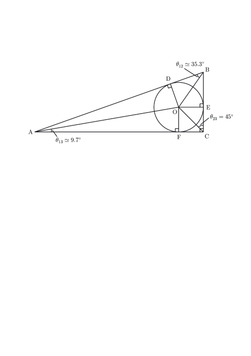
  Figure 3: A geometrical description of the sum rules $\theta_{12}+\theta_{13}=\theta_{23}$ and $\theta_{12}+\theta_{13}+\theta_{23}=90^{\circ}$ for the correlative neutrino mixing pattern in terms of the inner angles of the right triangle $\triangle\rm ABC$.

  The other pattern of $U_{0}$ is the tetra-maximal mixing pattern [109]

  $$U_{0}=\left(\begin{matrix}\frac{2+\sqrt{2}}{4}&\frac{1}{2}&\frac{2-\sqrt{2}}{4}\cr-\frac{\sqrt{2}}{4}+\frac{i\left(\sqrt{2}-1\right)}{4}&\frac{1}{2}-\frac{i\sqrt{2}}{4}&\frac{\sqrt{2}}{4}+\frac{i\left(\sqrt{2}+1\right)}{4}\cr-\frac{\sqrt{2}}{4}-\frac{i\left(\sqrt{2}-1\right)}{4}&\frac{1}{2}+\frac{i\sqrt{2}}{4}&\frac{\sqrt{2}}{4}-\frac{i\left(\sqrt{2}+1\right)}{4}\cr\end{matrix}\right)\;,$$ (32)

  which predicts $\theta^{(0)}_{12}=\arctan(2-\sqrt{2})\simeq 30.4^{\circ}$, $\theta^{(0)}_{23}=45^{\circ}$ and $\theta^{(0)}_{13}=\arcsin[(2-\sqrt{2})/4]\simeq 8.4^{\circ}$. Of course, whether such constant mixing patterns can easily be derived from some underlying flavor symmetries remains an open question.

In short, today’s model building has to take the challenge caused by the reasonably large value of $\theta_{13}$.

Note that the RGE running effects or finite quantum corrections are not easy to generate $\theta_{13}\simeq 9^{\circ}$ from $\theta^{(0)}_{13}=0^{\circ}$, unless the seesaw threshold effects or other extreme conditions are taken into account [110, 111, 112, 113, 114, 115, 116, 117, 118, 119]. One may therefore consider a pattern of $U_{0}$ with nonzero $\theta^{(0)}_{13}$, such as the tetra-maximal mixing pattern [120] or the correlative mixing pattern [121], as a starting point of view to calculate the radiative corrections before confronting it with current experimental data. We shall elaborate on this point in detail in section 5.

4.3 The Minimal Perturbation to $U_{0}$

Note that the perturbation matrix $\Delta U$ in Eq. (17) is in general a sum of all possible perturbations to the constant flavor mixing matrix $U_{0}$. From the point of view of model building, it is helpful to single out a viable $\Delta U$ whose form is as simple as possible. To do so, let us reexpress Eq. (17) in the following manner:

$$U=\left(U_{0}+\Delta U\right)P_{\nu}=U_{0}\left({\bf 1}+\Delta U^{\prime}\right)P_{\nu}=\left({\bf 1}+\Delta U^{\prime}_{\rm L}\right)U_{0}\left({\bf 1}+\Delta U^{\prime}_{\rm R}\right)P_{\nu}\;,$$ (33)

where $\Delta U=U_{0}\Delta U^{\prime}=\Delta U^{\prime}_{\rm L}U_{0}+U_{0}\Delta U^{\prime}_{\rm R}+\Delta U^{\prime}_{\rm L}U_{0}\Delta U^{\prime}_{\rm R}$ holds, and it satisfies the condition $U_{0}\Delta U^{\dagger}+\Delta UU^{\dagger}_{0}+\Delta U\Delta U^{\dagger}={\bf 0}$ as a result of the unitarity of $U$ itself. Therefore, one may achieve a viable but minimal perturbation to $U_{0}$ by switching off $\Delta U^{\prime}_{\rm L}$ (or $\Delta U^{\prime}_{\rm R}$) and adjusting $\Delta U^{\prime}_{\rm R}$ (or $\Delta U^{\prime}_{\rm L}$) to its simplest form which is allowed by current experimental data. Such a treatment is actually equivalent to multiplying $U_{0}$ by a unitary perturbation matrix, which may more or less deviate from the unit matrix $\bf 1$, from either its left-hand side or its right-hand side. The first example of this kind was given before [73, 91, 92] for the democratic mixing pattern, and its $\Delta U$ was mainly responsible for the generation of nonzero $\theta_{13}$ and $\delta$.

Here we concentrate on the typical patterns of $U_{0}$ discussed above and outline the main ideas of choosing the minimal perturbations to them.

• If $U_{0}$ predicts $\theta^{(0)}_{23}=45^{\circ}$ and $\theta^{(0)}_{13}=0^{\circ}$ together with $\theta^{(0)}_{12}>34^{\circ}$ (the best-fit value based on current neutrino oscillation data [55]), then the simplest way to generate a relatively large $\theta_{13}$, keep $\theta_{23}=\theta^{(0)}_{23}=45^{\circ}$ unchanged and correct $\theta^{(0)}_{12}$ to a slightly smaller value is to choose a complex $(2,3)$ rotation matrix as the perturbation matrix:

  $${\bf 1}+\Delta U^{\prime}=\left(\begin{matrix}1&0&0\cr 0&\cos\theta&i\sin\theta\cr 0&i\sin\theta&\cos\theta\cr\end{matrix}\right)~{}~{}{\rm or}~{}~{}\Delta U^{\prime}\simeq\left(\begin{matrix}0&0&0\cr 0&-\frac{1}{2}\sin^{2}\theta&i\sin\theta\cr 0&i\sin\theta&-\frac{1}{2}\sin^{2}\theta\cr\end{matrix}\right)\;,$$ (34)

  where $\theta$ is a small angle to trigger the perturbation effect. The most striking example in this category is to take $U_{0}$ to be the tri-bimaximal mixing pattern given in Eq. (24). The result is [122, 123]:

  $$U=\left(\begin{matrix}\frac{\sqrt{2}}{\sqrt{3}}&\frac{1}{\sqrt{3}}\cos\theta&\frac{i}{\sqrt{3}}\sin\theta\cr-\frac{1}{\sqrt{6}}&\frac{1}{\sqrt{3}}\cos\theta+\frac{i}{\sqrt{2}}\sin\theta&\frac{1}{\sqrt{2}}\cos\theta+\frac{i}{\sqrt{3}}\sin\theta\cr\frac{1}{\sqrt{6}}&-\frac{1}{\sqrt{3}}\cos\theta+\frac{i}{\sqrt{2}}\sin\theta&\frac{1}{\sqrt{2}}\cos\theta-\frac{i}{\sqrt{3}}\sin\theta\cr\end{matrix}\right)P_{\nu}\;,$$ (35)

  which predicts

  $$\sin^{2}\theta_{12}=\frac{1}{3}\left(1-2\tan^{2}\theta_{13}\right)\;,~{}\sin^{2}\theta_{13}=\frac{1}{3}\sin^{2}\theta\;,~{}\theta_{23}=45^{\circ}\;,~{}\delta=90^{\circ}\;$$ (36)

  in the standard parametrization. Note that the obtained correlation between $\theta_{12}$ and $\theta_{13}$ is especially interesting because it leads us to $\theta_{12}\to 34^{\circ}$ when $\theta_{13}\to 9^{\circ}$, consistent with the present experimental data. If $\theta_{23}$ is allowed to slightly deviate from $\theta^{(0)}_{23}=45^{\circ}$, then one may simply make the replacement $i\to e^{i\delta}$ in Eq. (35).

• If $U_{0}$ predicts $\theta^{(0)}_{23}=45^{\circ}$ and $\theta^{(0)}_{13}=0^{\circ}$ together with $\theta^{(0)}_{12}<34^{\circ}$, then the most economical way to generate a relatively large $\theta_{13}$, keep $\theta_{23}=\theta^{(0)}_{23}=45^{\circ}$ unchanged and correct $\theta^{(0)}_{12}$ to a slightly larger value is to choose a complex $(1,3)$ rotation matrix as the perturbation matrix:

  $${\bf 1}+\Delta U^{\prime}=\left(\begin{matrix}\cos\theta&0&i\sin\theta\cr 0&1&0\cr i\sin\theta&0&\cos\theta\cr\end{matrix}\right)~{}~{}{\rm or}~{}~{}\Delta U^{\prime}\simeq\left(\begin{matrix}-\frac{1}{2}\sin^{2}\theta&0&i\sin\theta\cr 0&0&0\cr i\sin\theta&0&-\frac{1}{2}\sin^{2}\theta\cr\end{matrix}\right)\;.$$ (37)

  Taking $U_{0}$ to be the golden-ratio mixing pattern in Eq. (26), we immediately arrive at

  $$U=\left(\begin{matrix}\frac{\sqrt{2}}{\sqrt{5-\sqrt{5}}}\cos\theta&\frac{\sqrt{2}}{\sqrt{5+\sqrt{5}}}&\frac{i\sqrt{2}}{\sqrt{5-\sqrt{5}}}\sin\theta\cr-\frac{1}{\sqrt{5+\sqrt{5}}}\cos\theta+\frac{i}{\sqrt{2}}\sin\theta&\frac{1}{\sqrt{5-\sqrt{5}}}&\frac{1}{\sqrt{2}}\cos\theta-\frac{i}{\sqrt{5+\sqrt{5}}}\sin\theta\cr\frac{1}{\sqrt{5+\sqrt{5}}}\cos\theta+\frac{i}{\sqrt{2}}\sin\theta&-\frac{1}{\sqrt{5-\sqrt{5}}}&\frac{1}{\sqrt{2}}\cos\theta+\frac{i}{\sqrt{5+\sqrt{5}}}\sin\theta\cr\end{matrix}\right)P_{\nu}\;,$$ (38)

  whose predictions include $\theta_{23}=45^{\circ}$, $\delta=90^{\circ}$, and

  $$\sin^{2}\theta_{12}=\frac{2}{5+\sqrt{5}}\left(1+\tan^{2}\theta_{13}\right)\;,~{}~{}~{}~{}~{}\sin^{2}\theta_{13}=\frac{2}{5-\sqrt{5}}\sin^{2}\theta$$ (39)

  in the standard parametrization of $U$. In this case the correlation between $\theta_{12}$ and $\theta_{13}$ leads to $\theta_{12}\to 32^{\circ}$ when $\theta_{13}\to 9^{\circ}$, compatible with the experimental data. Again, the replacement $i\to e^{i\delta}$ in Eq. (38) allows one to obtain a somewhat more flexible value of $\theta_{23}$ which may slightly deviate from $\theta^{(0)}_{23}=45^{\circ}$.

• If $U_{0}$ is quite far away from the realistic MNSP matrix $U$, one has to consider a somewhat complicated perturbation matrix including two rotation angles. In the neglect of CP violation, for instance, we may consider

  $${\bf 1}+\Delta U^{\prime}=\left(\begin{matrix}c^{\prime}_{12}&-s^{\prime}_{12}&0\cr s^{\prime}_{12}c^{\prime}_{23}&c^{\prime}_{12}c^{\prime}_{23}&s^{\prime}_{23}\cr s^{\prime}_{12}s^{\prime}_{23}&c^{\prime}_{12}s^{\prime}_{23}&-c^{\prime}_{23}\cr\end{matrix}\right)\;,$$ (40)

  where $c^{\prime}_{ij}\equiv\cos\theta^{\prime}_{ij}$ and $s^{\prime}_{ij}\equiv\sin\theta^{\prime}_{ij}$ (for $ij=12,23$). However, we hope that the resulting structure of $U$ still allows us to obtain one or two predictions, in particular for the mixing angle $\theta_{13}$. A simple example of this kind has been given before [124] by taking $U_{0}$ to be the democratic mixing pattern, and it predicts an interesting relationship between $\theta_{13}$ and $\theta_{23}$ in the standard parametrization:

  $$\sin\theta_{13}=\frac{\sqrt{2}-\tan\theta_{23}}{\sqrt{5-2\sqrt{2}\tan\theta_{23}+4\tan^{2}\theta_{23}}}\;.$$ (41)

  Typically taking $\theta_{23}\simeq 45^{\circ}$, we can arrive at $\theta_{13}\simeq 9.6^{\circ}$ [124]. It is certainly easy to accommodate a CP-violating phase in $\Delta U^{\prime}$, although its form might not be really minimal anymore.

For those constant flavor mixing patterns with $\theta^{(0)}_{13}\neq 0^{\circ}$ from the very beginning, such as the correlative [106] and tetra-maximal [109] mixing scenarios given in Eqs. (30) and (32), the similar minimal perturbations can be introduced in order to make the resulting MNSP matrix $U$ fit the experimental data to a better degree of accuracy.

It should be noted that the above discussions about possible patterns of $\Delta U$ (or $\Delta U^{\prime}$) with respect to those of $U_{0}$ are purely phenomenological. From the point of view of model building, it is more meaningful to consider the textures of lepton mass matrices

$$M_{l}=M^{(0)}_{l}+\Delta M_{l}\;,~{}~{}~{}~{}~{}~{}~{}~{}~{}~{}~{}~{}M_{\nu}=M^{(0)}_{\nu}+\Delta M_{\nu}\;,$$ (42)

where $M^{(0)}_{l}$ and $M^{(0)}_{\nu}$ can be obtained in the limit of certain flavor symmetries, and their special structures allow us to achieve a constant flavor mixing pattern $U_{0}$. The perturbation matrices $\Delta M_{l}$ and $\Delta M_{\nu}$ play an important role in transforming $U_{0}$ into the realistic MNSP matrix $U$, and thus their textures should be determined in a simple way and with a good reason. The connection between $\Delta M_{l,\nu}$ and $\Delta U$ (or $\Delta U^{\prime}$) depends on the details of a lepton flavor model and may not be very transparent in most cases. In the basis where $M_{l}$ is real and positive, however, $\Delta M_{\nu}$ can be formally expressed as

$$\Delta M_{\nu}=\left(U_{0}+\Delta U\right)\overline{M}_{\nu}\left(U_{0}+\Delta U\right)^{T}-U_{0}\overline{M}^{(0)}_{\nu}U^{T}_{0}\;,$$ (43)

where $\overline{M}_{\nu}=P_{\nu}\widehat{M}_{\nu}P^{T}_{\nu}$ and $\overline{M}^{(0)}_{\nu}=P^{\prime}_{\nu}\widehat{M}^{\prime}_{\nu}P^{\prime T}_{\nu}$, $\widehat{M}^{\prime}_{\nu}\equiv{\rm Diag}\{m^{\prime}_{1},m^{\prime}_{2},m^{\prime}_{3}\}$ and $P^{\prime}_{\nu}\equiv{\rm Diag}\{e^{i\rho^{\prime}},e^{i\sigma^{\prime}},1\}$. Here $m^{\prime}_{i}$ (for $i=1,2,3$) denote the eigenvalues of $M^{(0)}_{\nu}$ in the symmetry limit, while $\rho^{\prime}$ and $\sigma^{\prime}$ stand for the Majorana phases in the same limit. It is therefore possible, at least in principle, to fix the structure of $\Delta M_{\nu}$ with the help of a certain flavor symmetry and current experimental data.

5 UNSUPPRESSED $\theta_{13}$ AND RGE RUNNING EFFECTS

The RGE running effects of the neutrino flavor parameters have been discussed in many papers [110, 111, 112, 113, 114, 115, 116, 117, 118, 119, 125, 126, 127, 128, 129, 130, 131, 132, 133, 134]. It is known that large radiative corrections to those parameters are possible, especially when the neutrino masses are nearly degenerate or the value of $\tan\beta$ is sufficiently big in the MSSM. The fact that $\theta_{13}$ is not as small as previously expected motivates one to reconsider how it can be generated at the tree level or by quantum corrections. Some studies in this regard have recently been done to look at the impacts of a relatively large $\theta_{13}$ on the running behaviors of the other two mixing angles and the CP-violating phases [121].

5.1 Approximate RGEs

The masses of the Majorana neutrinos are believed to be attributed to some underlying new physics at a superhigh-energy scale $\Lambda$ (e.g., via the canonical seesaw mechanism [20, 21, 22, 23, 24]). But this kind of new physics can all point to the unique dimension-5 Weinberg operator for the neutrino masses in an effective field theory after the corresponding heavy degrees of freedom are integrated out [135]. In the MSSM, such a dimension-5 operator reads

$$\frac{{\cal L}_{\rm d=5}}{\Lambda} = \frac{1}{2}\;\overline{\ell_{\rm L}}H_{2}\cdot\kappa\cdot H^{T}_{2}\ell^{c}_{\rm L}\;+\;{\rm h.c.}\;,$$ (44)

where $\Lambda$ denotes the cutoff scale, $\ell_{\rm L}$ stands for the left-handed lepton doublet, $H_{2}$ is one of the MSSM Higgs doublets, and $\kappa$ represents the effective neutrino coupling matrix. One may obtain the effective Majorana neutrino mass matrix $M_{\nu}=\kappa v^{2}\tan^{2}\beta/(1+\tan^{2}\beta)$ after spontaneous gauge symmetry breaking. The cutoff scale $\Lambda$ implies the scale of new physics, such as the mass scale of the heavy Majorana neutrinos in the canonical seesaw mechanism. The evolution of $\kappa$ from $\Lambda$ down to the electroweak scale $\Lambda_{\rm EW}$ is formally independent of any details of the relevent model from which $\kappa$ is derived. Below $\Lambda$ the scale dependence of $\kappa$ is described by

$$16\pi^{2}\frac{{\rm d}\kappa}{{\rm d}t}\;=\;\alpha_{\rm M}\kappa+\left[\left(Y_{l}Y^{\dagger}_{l}\right)\kappa+\kappa\left(Y_{l}Y^{\dagger}_{l}\right)^{T}\right]\;$$ (45)

at the one-loop level in the MSSM [125, 126, 128], where $\alpha_{\rm M}\approx-1.2g^{2}_{1}-6g^{2}_{2}+6y^{2}_{t}$.

One may use Eq. (45) to derive the explicit RGEs of the three neutrino masses and six flavor mixing parameters [113, 114, 125, 126, 128, 131]. Given an approximate mass degeneracy of the three neutrinos together with the standard parametrization of the MNSP matrix $U$ in Eq. (2), the RGEs of $m_{i}$ (for $i=1,2,3$) turn out to be

$$\frac{{\rm d}m_{1}}{{\rm d}t} \approx \frac{m_{1}}{16\pi^{2}}\left[\alpha_{\rm M}+2y^{2}_{\tau}\left(s^{2}_{12}s^{2}_{23}-2c_{\delta}c_{12}c_{23}s_{12}s_{23}s_{13}+{\cal O}(s^{2}_{13})\right)\right]\;,$$

$$\frac{{\rm d}m_{2}}{{\rm d}t} \approx \frac{m_{2}}{16\pi^{2}}\left[\alpha_{\rm M}+2y^{2}_{\tau}\left(c^{2}_{12}s^{2}_{23}+2c_{\delta}c_{12}c_{23}s_{12}s_{23}s_{13}+{\cal O}(s^{2}_{13})\right)\right]\;,$$

$$\frac{{\rm d}m_{3}}{{\rm d}t} \approx \frac{m_{3}}{16\pi^{2}}\left[\alpha_{\rm M}+2y^{2}_{\tau}c^{2}_{23}+{\cal O}(s^{2}_{13})\right]\;.$$ (46)

The RGEs of $\theta_{ij}$ (for $ij=12,23,13$) are found to be

$$\frac{{\rm d}\theta_{12}}{{\rm d}t} \approx -\frac{y^{2}_{\tau}}{4\pi^{2}}\left\{\frac{m^{2}_{1}}{\Delta m^{2}_{21}}s_{23}\left[\left(c_{12}s_{12}s_{23}-\cos 2\theta_{12}c_{23}s_{13}c_{\delta}\right)c_{(\rho-\sigma)}\right.\right.$$

$$~{}~{}~{}~{}~{}~{}~{}~{}~{}~{}~{}~{}~{}~{}~{}~{}~{}~{}~{}~{}~{}\left.\left.+c_{23}s_{13}s_{\delta}s_{(\rho-\sigma)}\right]c_{(\rho-\sigma)}\right.$$

$$~{}~{}~{}\left.-\frac{m^{2}_{1}}{\Delta m^{2}_{32}}c_{23}s_{23}s_{13}\left(s^{2}_{12}c_{(\delta+\rho)}c_{\rho}+c^{2}_{12}c_{(\delta+\sigma)}c_{\sigma}\right)+{\cal O}(s^{2}_{13})\right\}\;,$$

$$\frac{{\rm d}\theta_{23}}{{\rm d}t} \approx -\frac{y^{2}_{\tau}}{4\pi^{2}}\frac{m^{2}_{1}}{\Delta m^{2}_{32}}c_{23}\left[s_{23}\left(s^{2}_{12}c^{2}_{\rho}+c^{2}_{12}c^{2}_{\sigma}\right)\right.$$

$$~{}~{}~{}\left.-\frac{1}{2}c_{12}s_{12}c_{23}s_{13}\left(c_{(\delta+2\rho)}-c_{(\delta+2\sigma)}\right)+{\cal O}(s^{2}_{13})\right]\;,$$

$$\frac{{\rm d}\theta_{13}}{{\rm d}t} \approx \frac{y^{2}_{\tau}}{8\pi^{2}}\frac{m^{2}_{1}}{\Delta m^{2}_{32}}c_{23}c_{13}\left[c_{12}s_{12}s_{23}\left(c_{(\delta+2\rho)}-c_{(\delta+2\sigma)}\right)\right.$$ (47)

$$\left.~{}~{}~{}-2c_{23}s_{13}\left(c^{2}_{12}c^{2}_{(\delta+\rho)}+s^{2}_{12}c^{2}_{(\delta+\sigma)}\right)+{\cal O}(s^{2}_{13})\right]\;,$$

in which $c_{x}\equiv\cos x$ and $s_{x}\equiv\sin x$ (for $x=\delta,\;\rho,\;\sigma,\;\rho-\sigma,\;\delta+\rho,\;\delta+\sigma,\;\delta+2\rho,\;\delta+2\sigma$). The RGEs of the three CP-violating phases $\delta$, $\rho$ and $\sigma$ can be written as

$$\frac{{\rm d}\delta}{{\rm d}t} \approx -\frac{y^{2}_{\tau}}{4\pi^{2}}\left\{\frac{m^{2}_{1}}{\Delta m^{2}_{21}}s_{23}\left[\left(s_{23}-\frac{\cos 2\theta_{12}c_{23}s_{13}c_{\delta}}{c_{12}s_{12}}\right)c_{(\rho-\sigma)}\right.\right.$$

$$~{}~{}~{}~{}~{}~{}~{}~{}~{}~{}~{}~{}~{}~{}~{}\left.\left.+\frac{c_{23}s_{13}s_{\delta}}{c_{12}s_{12}}s_{(\rho-\sigma)}+{\cal O}(s^{2}_{13})\right]s_{(\rho-\sigma)}\right.$$

$$~{}~{}~{}\left.-\frac{m^{2}_{1}}{\Delta m^{2}_{32}}s^{-1}_{13}\left[\frac{1}{2}c_{12}s_{12}c_{23}s_{23}\left(s_{(\delta+2\rho)}-s_{(\delta+2\sigma)}\right)\right.\right.$$

$$~{}~{}~{}~{}~{}~{}~{}~{}~{}~{}~{}~{}\left.\left.+\left(c_{(\delta-\rho)}s_{(\delta-\rho)}s^{2}_{12}+c_{(\delta-\sigma)}s_{(\delta-\sigma)}c^{2}_{12}\right)\cos 2\theta_{23}s_{13}\right.\right.$$

$$~{}~{}~{}~{}~{}~{}~{}~{}~{}~{}~{}~{}\left.\left.+\left(c_{\rho}s_{\rho}c^{2}_{12}+c_{\sigma}s_{\sigma}s^{2}_{12}\right)c^{2}_{23}s_{13}+{\cal O}(s^{2}_{13})\right]\right\}\;,$$

$$\frac{{\rm d}\rho}{{\rm d}t} \approx \frac{y^{2}_{\tau}}{4\pi^{2}}\left\{\frac{m^{2}_{1}}{\Delta m^{2}_{21}}s_{23}c^{2}_{12}\left[\left(s_{23}-\frac{\cos 2\theta_{12}c_{23}s_{13}c_{\delta}}{c_{12}s_{12}}\right)c_{(\rho-\sigma)}\right.\right.$$

$$~{}~{}~{}~{}~{}~{}~{}~{}~{}~{}~{}~{}~{}~{}~{}\left.\left.+\frac{c_{23}s_{13}s_{\delta}}{c_{12}s_{12}}s_{(\rho-\sigma)}+{\cal O}(s^{2}_{13})\right]s_{(\rho-\sigma)}\right.$$

$$\left.-\frac{m^{2}_{1}}{\Delta m^{2}_{32}}s^{-1}_{13}\left[\left(c_{(\delta-\rho)}s_{(\delta-\rho)}s^{2}_{12}+c_{(\delta-\sigma)}s_{(\delta-\sigma)}c^{2}_{12}\right)\cos 2\theta_{23}s_{13}+{\cal O}(s^{2}_{13})\right]\right\}\;,$$

$$\frac{{\rm d}\sigma}{{\rm d}t} \approx \frac{y^{2}_{\tau}}{4\pi^{2}}\left\{\frac{m^{2}_{1}}{\Delta m^{2}_{21}}s_{23}s^{2}_{12}\left[\left(s_{23}-\frac{\cos 2\theta_{12}c_{23}s_{13}c_{\delta}}{c_{12}s_{12}}\right)c_{(\rho-\sigma)}\right.\right.$$

$$~{}~{}~{}~{}~{}~{}~{}~{}~{}~{}~{}~{}~{}~{}~{}\left.\left.+\frac{c_{23}s_{13}s_{\delta}}{c_{12}s_{12}}s_{(\rho-\sigma)}+{\cal O}(s^{2}_{13})\right]s_{(\rho-\sigma)}\right.$$

$$\left.-\frac{m^{2}_{1}}{\Delta m^{2}_{32}}s^{-1}_{13}\left[\left(c_{(\delta-\rho)}s_{(\delta-\rho)}s^{2}_{12}+c_{(\delta-\sigma)}s_{(\delta-\sigma)}c^{2}_{12}\right)\cos 2\theta_{23}s_{13}+{\cal O}(s^{2}_{13})\right]\right\}\;.$$

In addition, the RGE of ${\cal J}$ is obtained as follows:

$$\frac{\rm d}{{\rm d}t}\;{\cal J} \approx -\frac{y^{2}_{\tau}}{8\pi^{2}}\left\{\frac{m^{2}_{1}}{\Delta m^{2}_{21}}\left[{\cal J}\cos 2\theta_{12}s^{2}_{23}-\cos^{2}2\theta_{12}c^{2}_{23}s^{2}_{23}c^{2}_{13}s^{2}_{13}c_{\delta}s_{\delta}\right]\right.$$ (49)

$$~{}~{}~{}~{}~{}~{}\left.+\;\frac{m^{2}_{1}}{\Delta m^{2}_{32}}{\cal J}\cos 2\theta_{23}+{\cal O}(s^{3}_{13})\right\}\;.$$

The running behaviors of the three mixing angles and three CP-violating phases for a very small $\theta_{13}$ can be very different from those for a relative large $\theta_{13}$. In particular, the CP-violating phases play a crucial role in the RGEs. Let us elaborate on this point in the following.

5.2 Flavor Mixing Angles and CP-violating Phases

(1) The running behaviors of the three mixing angles. Eq. (47) shows that the RGE running behaviors of the three neutrino mixing angles are strongly dependent on the three CP-violating phases. As for the Majorana neutrinos, the radiative corrections to the three mixing angles can be adjusted by choosing different values of the CP-violating phases $\delta$, $\rho$ and $\sigma$. A numerical analysis has been carried out to look at their numerical evolution to $\Lambda_{\rm FS}$ via the RGEs in the MSSM with $\tan\beta=10$ (denoted as “MSSM10” for short) or $\tan\beta=50$ (denoted as “MSSM50” for short), in which $\theta_{12}=34^{\circ}$, $\theta_{23}=46^{\circ}$, $\theta_{13}=9^{\circ}$ are taken as the typical input and the three CP-violating phases are freely adjusted at $\Lambda_{\rm EW}$ [121]. The main results are summarized in Table 2, where the upper (lower) lines show the possible ranges of three mixing angles at $\Lambda_{\rm FS}$ for the normal (inverted) neutrino mass hierarchy.

The radiative corrections to the three mixing angles from $\Lambda_{\rm EW}\sim 10^{2}$ GeV to $\Lambda_{\rm FS}\sim 10^{14}$ GeV in the MSSM with $\tan\beta=10$ or $50$, where the three CP-violating phases are freely adjusted. Parameter Input ($\Lambda_{\rm EW}$) Output ($\Lambda_{\rm FS}$) MSSM10 MSSM50   $\theta_{12}$   $34.0^{\circ}$ $7^{\circ}$ to $55^{\circ}$ $0.5^{\circ}$ to $62^{\circ}$ (NH) $2^{\circ}$ to $31^{\circ}$ $2^{\circ}$ to $45^{\circ}$ (IH)   $\theta_{23}$   $46.0^{\circ}$ $47^{\circ}$ to $48.5^{\circ}$ $7.5^{\circ}$ to $45.5^{\circ}$ (NH) $43.5^{\circ}$ to $45^{\circ}$ $46.5^{\circ}$ to $89^{\circ}$ (IH)   $\theta_{13}$   $9.0^{\circ}$ $8.5^{\circ}$ to $10^{\circ}$ $2^{\circ}$ to $23^{\circ}$ (NH) $7.5^{\circ}$ to $9.5^{\circ}$ $7.5^{\circ}$ to $82^{\circ}$ (IH)

The RGE of $\theta_{12}$ is dominated by the term $\displaystyle-\frac{y^{2}_{\tau}}{8\pi^{2}}\frac{m^{2}_{1}}{\Delta m^{2}_{21}}c_{12}s_{12}s^{2}_{23}c^{2}_{(\rho-\sigma)}$, implying that the magnitude of the radiative correction to $\theta_{12}$ depends strongly on the phase difference $(\rho-\sigma)$. Hence $\theta_{12}$ is most sensitive to the RGE effect when $\rho\simeq\sigma$ holds. Running from $\Lambda_{\rm FS}\sim 10^{14}$ GeV down to $\Lambda_{\rm EW}$, the mixing angles $\theta_{23}$ and $\theta_{13}$ receive less significant radiative corrections in the MSSM10 case, as shown in Table 2. While in the MSSM50 case $\theta_{23}$ and $\theta_{13}$ may also receive significant radiative corrections if three CP-violating phases are well turned.

We have seen that the values of the three CP-violating phases are crucial for the evolution of the three mixing angles. A very special case is $(\rho-\sigma)\simeq\pm 90^{\circ}$, which leads us to

$$\frac{{\rm d}\theta_{12}}{{\rm d}t} \approx \frac{y^{2}_{\tau}}{4\pi^{2}}\frac{m^{2}_{1}}{\Delta m^{2}_{32}}c_{23}s_{23}s_{13}\left(s^{2}_{12}c_{(\delta+\rho)}c_{\rho}+c^{2}_{12}s_{(\delta+\rho)}s_{\rho}\right)\;,$$

$$\frac{{\rm d}\theta_{23}}{{\rm d}t} \approx -\frac{y^{2}_{\tau}}{4\pi^{2}}\frac{m^{2}_{1}}{\Delta m^{2}_{32}}c_{23}\left[s_{23}\left(s^{2}_{12}c^{2}_{\rho}+c^{2}_{12}s^{2}_{\rho}\right)-c_{12}s_{12}c_{23}s_{13}c_{(\delta+2\rho)}\right]\;,$$

$$\frac{{\rm d}\theta_{13}}{{\rm d}t} \approx \frac{y^{2}_{\tau}}{4\pi^{2}}\frac{m^{2}_{1}}{\Delta m^{2}_{32}}c_{23}c_{13}\left[c_{12}s_{12}s_{23}c_{(\delta+2\rho)}-c_{23}s_{13}\left(c^{2}_{12}c^{2}_{(\delta+\rho)}+s^{2}_{12}s^{2}_{(\delta+\rho)}\right)\right]\;.~{}~{}~{}~{}$$ (50)

Note that the term proportional to $m^{2}_{1}/\Delta m^{2}_{21}$ in the RGE of $\theta_{12}$ in Eq. (47) is suppressed by $\cos(\rho-\sigma)\simeq 0$ in this special case, and thus it has been omitted from Eq. (50). The three mixing angles may therefore receive comparably small radiative corrections for a modest value of $\tan\beta$ (e.g., in the MSSM10 case). This observation was not noticed in the literature simply because $\theta_{13}$ used to be assumed to be very small [125, 126, 127, 131]. If $\tan\beta$ is sufficiently large (e.g., in the MSSM50 case), however, the phase difference $(\rho-\sigma)$ will be able to quickly run away from its initial value $(\rho-\sigma)\sim\pm 90^{\circ}$ due to the significant radiative corrections, implying that Eq. (50) is no more a good approximation of Eq. (47).

Here let us consider a typical example of this special case — the correlative neutrino mixing pattern with $\theta_{12}\simeq 35.3^{\circ}$, $\theta_{23}=45^{\circ}$ and $\theta_{13}\simeq 9.7^{\circ}$ [106]. Compared with the best-fit values of the three mixing angles at $\Lambda_{\rm EW}$, the three mixing angles in this correlative mixing pattern at $\Lambda_{\rm FS}$ have to receive comparably small radiative corrections during their RGE evolution. As we have mentioned in the last paragraph, this requirement can easily be achieved in the MSSM10 case provided the condition $(\rho-\sigma)\simeq\pm 90^{\circ}$ is satisfied for a nearly degenerate neutrino mass spectrum. Such a condition is unnecessary if the neutrino mass spectrum has a strong hierarchy. The numerical results are presented in Table 3, where $\delta=-68^{\circ}$, $\rho=13^{\circ}$ and $\sigma=115^{\circ}$ are input at $\Lambda_{\rm FS}$. Then $\theta_{12}=34.52^{\circ}$, $\theta_{23}=45.98^{\circ}$ and $\theta_{13}=8.83^{\circ}$ are obtained at $\Lambda_{\rm EW}$ after the radiative corrections.

Radiative corrections to the correlative neutrino mixing pattern from $\Lambda_{\rm FS}\sim 10^{14}$ GeV to $\Lambda_{\rm EW}\sim 10^{2}$ GeV in the MSSM10. Parameter Input ($\Lambda_{\rm FS}$) Output ($\Lambda_{\rm EW}$) $m_{1}~{}({\rm eV})$ 0.227 0.200 $\Delta m^{2}_{21}~{}(10^{-5}~{}{\rm eV}^{2})$ 15.72 7.59 $\Delta m^{2}_{31}~{}(10^{-3}~{}{\rm eV}^{2})$ 3.19 2.40 $\theta_{12}$ $35.3^{\circ}$ $34.52^{\circ}$ $\theta_{23}$ $45^{\circ}$ $45.98^{\circ}$ $\theta_{13}$ $9.7^{\circ}$ $8.83^{\circ}$ $\delta$ $-68^{\circ}$ $-80.88^{\circ}$ $\rho$ $13^{\circ}$ $19.64^{\circ}$ $\sigma$ $115^{\circ}$ $118.03^{\circ}$ $\delta+\rho+\sigma$ $60^{\circ}$ $56.79^{\circ}$

(2) The radiative generation of the CP-violating phases. It is well known that one CP-violating phase can be generated from another [136], simply because they are entangled in the RGEs. An especially interesting example is the Dirac phase $\delta$, which measures the strength of CP violation in neutrino oscillations at the electroweak scale, can be radiatively generated from the nonzero Majorana phases $\rho$ and $\sigma$ at a superhigh-energy scale. If $\theta_{13}$ is very small, however, the running of $\delta$ can be significantly enhanced by the terms that are inversely proportional to $\sin\theta_{13}$. In the MSSM10 case it has been found that even $\delta=90^{\circ}$ can be radiatively generated if $\theta_{13}\simeq 1^{\circ}$ is taken [136]. Given $\theta_{13}\simeq 9^{\circ}$ at $\Lambda_{\rm EW}$, it is found that $-30^{\circ}\leq\delta\leq 30^{\circ}$ at $\Lambda_{\rm EW}$ may result from $\delta=0^{\circ}$ at $\Lambda_{\rm FS}$ in the MSSM10 case. In the MSSM50 case even $|\delta|\simeq 90^{\circ}$ can be obtained at $\Lambda_{\rm EW}$ [121].

(3) The running of the sum $\delta+\rho+\sigma$. Eq. (48) leads us to the RGE of the sum of the three CP-violating phases:

$$\frac{{\rm d}}{{\rm d}t}(\delta+\rho+\sigma) \approx \frac{y^{2}_{\tau}}{4\pi^{2}}\frac{m^{2}_{1}}{\Delta m^{2}_{32}}\frac{1}{s_{13}}\left[\frac{1}{2}c_{12}s_{12}c_{23}s_{23}\left(s_{(\delta+2\rho)}-s_{(\delta+2\sigma)}\right)\right.$$ (51)

$$~{}~{}~{}\left.-\left(c_{(\delta-\rho)}s_{(\delta-\rho)}s^{2}_{12}+c_{(\delta-\sigma)}s_{(\delta-\sigma)}c^{2}_{12}\right)\cos 2\theta_{23}s_{13}\right.$$

$$~{}~{}~{}\left.+\left(c_{\rho}s_{\rho}c^{2}_{12}+c_{\sigma}s_{\sigma}s^{2}_{12}\right)c^{2}_{23}s_{13}+{\cal O}(s^{2}_{13})\right]\;.$$

Since the value of $\theta_{13}$ is not small, the RGE running effect on $(\delta+\rho+\sigma)$ is expected to be insignificant. In other words, the sum of the three CP-violating phases may approximately keep unchanged during the RGE evolution in the SM or MSSM with a modest $\tan\beta$. The numerical analysis shows that $(\delta+\rho+\sigma)$ changes less than $4^{\circ}$ when running from $\Lambda_{\rm FS}$ down to $\Lambda_{\rm EW}$ in the MSSM10 case. The stability of $(\delta+\rho+\sigma)$ against the radiative corrections is quite impressive, unless $\tan\beta$ is sufficiently large [121].

To summarize, in order to obtain a phenomenologically-favored neutrino mixing pattern at the electroweak scale $\Lambda_{\rm EW}$, the radiative corrections should be carefully examined for those mixing patterns at a superhigh-energy scale $\Lambda_{\rm FS}$ which might result from a certain flavor symmetry. In the MSSM10 case the values of $\theta_{23}$ and $\theta_{13}$ predicted at $\Lambda_{\rm FS}$ are always close to their running values at $\Lambda_{\rm EW}$, while the value of $\theta_{12}$ at $\Lambda_{\rm FS}$ can be somewhat smaller or larger than its running value at $\Lambda_{\rm EW}$. In the MSSM50 case the allowed ranges of the three mixing angles at $\Lambda_{\rm FS}$ can be quite wide, as we have discussed above. However, a crucial point is that a given flavor symmetry model should be able to predict the appropriate CP-violating phases at $\Lambda_{\rm FS}$ in order to obtain the appropriate mixing angles at $\Lambda_{\rm EW}$ after the RGE evolution. In general, it is possible to generate $\theta_{13}\simeq 9^{\circ}$ at $\Lambda_{\rm EW}$ from $\theta_{13}\simeq 0^{\circ}$ at $\Lambda_{\rm FS}$ through the radiative corrections, in particular when some new degrees of freedom or nontrivial running effects (such as the seesaw threshold effects [113, 114, 131]) are taken into account or the three CP-violating phases are fine-turned. Therefore, we argue that it seems more natural for a specific flavor symmetry model to predict a relatively large $\theta_{13}$ at $\Lambda_{\rm FS}$.

A measurement of the Dirac phase $\delta$ in the forthcoming long-baseline neutrino oscillation experiments and any experimental information about the Majorana CP-violating phases $\rho$ and $\sigma$ are extremely important, so as to distinguish one flavor symmetry model from another through their different sensitivities to the radiative corrections. This observation makes sense in particular after the experimental errors associated with the neutrino mixing parameters are comparable with or smaller than the magnitudes of their respective RGE running effects.

6 SEESAW-ENHANCED NEUTRINO DIPOLE MOMENTS

The most popular mechanism of generating finite but tiny neutrino masses beyond the SM is the canonical seesaw mechanism [20, 21, 22, 23, 24], where the small neutrino masses are attributed to the existence of heavy degrees of freedom such as the right-handed Majorana neutrinos. In this elegant picture the $3\times 3$ MNSP matrix $U$ has a striking difference from the $3\times 3$ CKM matrix $V$ in the SM: it is not exactly unitary due to small mixing between light and heavy neutrinos as a result of the Yukawa interactions. The heavy neutrinos can be searched for at the LHC if the seesaw mechanism works at the TeV scale [137, 138, 139, 140], and the unitarity of $U$ can be tested in the future neutrino oscillation experiments. Another possibility is to look at the seesaw-induced non-unitary effects on the electromagnetic dipole moments (EMDMs) and radiative decays $\nu_{i}\to\nu_{j}+\gamma$ [141]. If the active neutrinos acquire their respective masses in the seesaw mechanism, they should have the EMDMs through quantum loops. The fact that the Majorana neutrinos are their own antiparticles implies that they can only have the transition EMDMs between two different neutrino mass eigenstates in an electric or magnetic field. The relevant radiative decays of the heavier active neutrinos, which may contribute to the cosmic infrared background in the Universe [142, 143, 144], are of particular interest in cosmology.

6.1 Analytical Discussions

We focus on the seesaw-induced non-unitary effects on the EMDMs and radiative decays of active Majorana neutrinos. The canonical seesaw mechanism is based on a simple extension of the SM in which three heavy right-handed neutrinos are added and the lepton number is violated by their Majorana mass term [20, 21, 22, 23, 24]:

$$-{\cal L}_{\nu}=\overline{\ell_{\rm L}}Y_{\nu}\tilde{H}N_{\rm R}+\frac{1}{2}\overline{N^{c}_{\rm R}}M_{\rm R}N_{\rm R}+{\rm h.c.}\;,$$ (52)

where $\tilde{H}\equiv i\sigma_{2}H^{*}$ with $H$ being the SM Higgs doublet, $\ell_{\rm L}$ denotes the left-handed lepton doublet, $N_{\rm R}$ stands for the column vector of three right-handed neutrinos, and $M_{\rm R}$ is a symmetric Majorana mass matrix. After spontaneous $SU(2)_{\rm L}\otimes U(1)_{\rm Y}\to U(1)_{\rm em}$ gauge symmetry breaking, $H$ achieves its vacuum expectation value $\langle H\rangle=v/\sqrt{2}$ with $v\simeq 246$ GeV. Then the Yukawa-interaction term in ${\cal L}_{\nu}$ yields the Dirac mass matrix $M_{\rm D}=Y_{\nu}v/\sqrt{2}$, but the Majorana mass term in ${\cal L}_{\nu}$ keeps unchanged since right-handed neutrinos are the $SU(2)_{\rm L}$ singlet and thus they are not subject to the electroweak symmetry breaking. The overall neutrino mass matrix turns out to be a symmetric $6\times 6$ matrix and can be diagonalized through

$${\cal U}^{\dagger}\left(\begin{matrix}{\bf 0}&M_{\rm D}\cr M^{T}_{\rm D}&M_{\rm R}\end{matrix}\right){\cal U}^{*}=\left(\begin{matrix}\widehat{M}_{\nu}&{\bf 0}\cr{\bf 0}&\widehat{M}_{N}\end{matrix}\right)\;,$$ (53)

where we have defined $\widehat{M}_{\nu}\equiv{\rm Diag}\{m_{1},m_{2},m_{3}\}$ and $\widehat{M}_{N}\equiv{\rm Diag}\{M_{1},M_{2},M_{3}\}$ with $m_{i}$ and $M_{i}$ being the physical masses of three light neutrinos $\nu_{i}$ and three heavy neutrinos $N_{i}$ (for $i=1,2,3$). The $6\times 6$ unitary matrix $\cal U$ is decomposed as [51]

$${\cal U}=\left(\begin{matrix}{\bf 1}&{\bf 0}\cr{\bf 0}&Z\cr\end{matrix}\right)\left(\begin{matrix}A&R\cr S&B\cr\end{matrix}\right)\left(\begin{matrix}X&{\bf 0}\cr{\bf 0}&{\bf 1}\cr\end{matrix}\right)\;,$$ (54)

where ${\bf 1}$ denotes the $3\times 3$ identity matrix, $X$ and $Z$ are the $3\times 3$ unitary matrices, and $A$, $B$, $R$ and $S$ are the $3\times 3$ matrices which characterize the correlation between the active or light neutrino sector ($X$) and the sterile or heavy neutrino sector ($Z$). A full parametrization of $\cal U$ in terms of 15 mixing angles and 15 CP-violating phases has been given before [51]. One may express the flavor eigenstates of three active neutrinos in terms of the mass eigenstates $\nu_{i}$ and $N_{i}$. In the mass basis of charged leptons and neutrinos, the leptonic weak charged-current (cc) and neutral-current (nc) interactions read

$$-{\cal L}_{\rm cc} = \frac{g}{\sqrt{2}}\left[\overline{l_{\alpha\rm L}}\gamma^{\mu}\left(U_{\alpha i}\nu_{i\rm L}+R_{\alpha i}N_{i\rm L}\right)W^{-}_{\mu}+{\rm h.c.}\right]\;,$$

$$-{\cal L}_{\rm nc} = \frac{g}{2\cos\theta_{\rm w}}\left\{\overline{\nu_{i\rm L}}\gamma^{\mu}(U^{\dagger}U)_{ij}\nu_{j\rm L}+\overline{N_{i\rm L}}\gamma^{\mu}(R^{\dagger}R)_{ij}N_{j\rm L}\right.$$ (55)

$$~{}~{}~{}~{}~{}~{}\left.+\left[\overline{\nu_{i\rm L}}\gamma^{\mu}(U^{\dagger}R)_{ij}N_{j\rm L}+{\rm h.c.}\right]\right\}Z_{\mu}\;,$$

where $\alpha$ runs over $e$, $\mu$ or $\tau$, $U=AX$ is responsible for the flavor mixing of active neutrinos $\nu_{i}$, and $R$ measures the strength of charged-current interactions of heavy neutrinos $N_{i}$ (for $i=1,2,3$) [145]. A small deviation of $U$ from $X$ is actually characterized by nonvanishing $R$, as $UU^{\dagger}=AA^{\dagger}={\bf 1}-RR^{\dagger}$ holds. The exact seesaw relation between the masses of light and heavy neutrinos is $U\widehat{M}_{\nu}U^{T}+R\widehat{M}_{N}R^{T}={\bf 0}$, which signifies the correlation between neutrino masses and flavor mixing parameters.

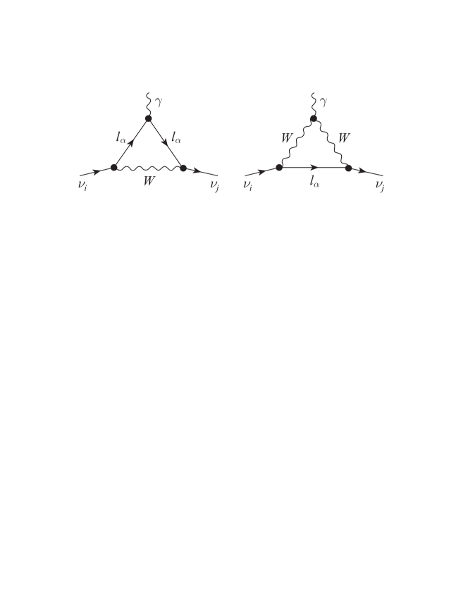
Figure 4: The one-loop Feynman diagrams (and their charge-conjugate counterparts) contributing to the EMDMs of the Majorana neutrinos, where $\alpha=e,\mu,\tau$ and $i,j=1,2,3$.

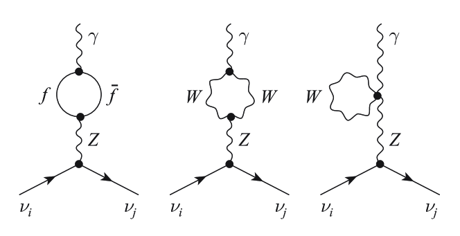
Figure 5: The one-loop $\gamma$-$Z$ self-energy diagrams (and their charge-conjugate counterparts) associated with the EMDMs of massive Majorana neutrinos, where $f$ denotes all the SM fermions and $i,j=1,2,3$.

Let us consider the radiative $\nu_{i}\to\nu_{j}+\gamma$ transition, whose electromagnetic vertex can be written as

$$\Gamma^{\mu}_{ij}(0)=\mu_{ij}\left(i\ \sigma^{\mu\nu}q_{\nu}\right)+\epsilon_{ij}\left(\sigma^{\mu\nu}q_{\nu}\gamma_{5}\right)\;$$ (56)

for a real photon satisfying the on-shell conditions $q^{2}=0$ and $q_{\mu}\varepsilon^{\mu}=0$. In Eq. (56) $\epsilon_{ij}$ and $\mu_{ij}$ are the electric and magnetic transition dipole moments of Majorana neutrinos, and their sizes can be calculated via the proper vertex diagrams in Fig. 4 (weak cc interactions). The $\gamma$-$Z$ self-energy diagrams in Fig. 5 (weak nc interactions) do not have any net contribution to $\epsilon_{ij}$ and $\mu_{ij}$, but we find that they play a very crucial role in eliminating the infinities because the divergent terms originating from Fig. 4 are unable to automatically cancel out in the presence of the seesaw-induced non-unitary effects (i.e., $R\neq{\bf 0}$ and $U\neq X$) unless those divergent terms originating from Fig. 5 are also taken into account. This observation is new. It implies that the non-unitary case under discussion is somewhat different from the unitary case (i.e., $R={\bf 0}$ and $U^{\dagger}U=X^{\dagger}X={\bf 1}$) discussed before in the literature [146, 147, 148, 149], where the Feynman diagrams in Fig. 5 are forbidden and the divergent terms arising from Fig. 4 can automatically cancel out.

After a careful calculation, we arrive at

$$\mu_{ij} = \frac{ieG_{\rm F}}{4\sqrt{2}\pi^{2}}\left(m_{i}+m_{j}\right)\sum_{\alpha}F_{\alpha}\text{Im}\left(U_{\alpha i}U^{*}_{\alpha j}\right)\;,$$

$$\epsilon_{ij} = \frac{eG_{\rm F}}{4\sqrt{2}\pi^{2}}\left(m_{i}-m_{j}\right)\sum_{\alpha}F_{\alpha}\text{Re}\left(U_{\alpha i}U^{*}_{\alpha j}\right)\;,$$ (57)

where

$$F_{\alpha}=\frac{3}{4}\left[\frac{2-\xi_{\alpha}}{1-\xi_{\alpha}}-\frac{2\xi_{\alpha}}{\left(1-\xi_{\alpha}\right)^{2}}+\frac{2\xi^{2}_{\alpha}\ln\xi_{\alpha}}{\left(1-\xi_{\alpha}\right)^{3}}\right]\;$$ (58)

with $\xi_{\alpha}\equiv m^{2}_{\alpha}/M^{2}_{W}$ (for $\alpha=e,\mu,\tau$) denotes the one-loop function. Although this result is formally the same as that obtained in the literature [146, 147, 148, 149], they are intrinsically different as the seesaw-induced non-unitary effects on $\mu_{ij}$ and $\epsilon_{ij}$ were not considered in the previous works. To see how important such non-unitary effects may be, let us make two analytical approximations. First, $F_{\alpha}\simeq 3\left(2-\xi_{\alpha}\right)/4$ holds to a good degree of accuracy for $\xi_{\alpha}\ll 1$. Second, $U=AX\simeq X-TX$ is also a good approximation for small non-unitary corrections to $X$, where [51]

$$X = \left(\begin{matrix}c_{12}c_{13}&\hat{s}^{*}_{12}c_{13}&\hat{s}^{*}_{13}\cr-\hat{s}_{12}c_{23}-c_{12}\hat{s}_{13}\hat{s}^{*}_{23}&c_{12}c_{23}-\hat{s}^{*}_{12}\hat{s}_{13}\hat{s}^{*}_{23}&c_{13}\hat{s}^{*}_{23}\cr\hat{s}_{12}\hat{s}_{23}-c_{12}\hat{s}_{13}c_{23}&-c_{12}\hat{s}_{23}-\hat{s}^{*}_{12}\hat{s}_{13}c_{23}&c_{13}c_{23}\cr\end{matrix}\right),$$

$$T = \left(\begin{matrix}\displaystyle\frac{1}{2}\sum^{6}_{k=4}s^{2}_{1k}&0&0\cr\displaystyle\sum^{6}_{k=4}\hat{s}_{1k}\hat{s}^{*}_{2k}&\displaystyle\frac{1}{2}\sum^{6}_{k=4}s^{2}_{2k}&0\cr\displaystyle\sum^{6}_{k=4}\hat{s}_{1k}\hat{s}^{*}_{3k}&\displaystyle\sum^{6}_{k=4}\hat{s}_{2k}\hat{s}^{*}_{3k}&\displaystyle\frac{1}{2}\sum^{6}_{k=4}s^{2}_{3k}\cr\end{matrix}\right)~{}$$ (59)

with $c_{ij}\equiv\cos\theta_{ij}$ and $\hat{s}_{ij}\equiv e^{i\delta_{ij}}\sin\theta_{ij}$ (here $\theta_{ij}$ and $\delta_{ij}$ are the mixing angles and CP-violating phases). Note that the light-heavy neutrino mixing angles $\theta_{ik}$ (for $i=1,2,3$ and $k=4,5,6$) are at most of ${\cal O}(0.1)$ [150], such that the deviation of $U$ from $X$ is at the percent level or much smaller. Then we obtain

$$\sum_{\alpha}F_{\alpha}\left(U_{\alpha i}U^{*}_{\alpha j}\right) \simeq -\frac{3}{2}\sum_{\alpha}\left[\left(X\right)_{\alpha i}\left(TX\right)^{*}_{\alpha j}+\left(TX\right)_{\alpha i}\left(X\right)^{*}_{\alpha j}\right]$$ (60)

$$-\frac{3}{4}\sum_{\alpha}\left[\xi_{\alpha}\left(X\right)_{\alpha i}\left(X\right)^{*}_{\alpha j}\right]\;.$$

The first and second terms on the right-hand side of this equation correspond to the non-unitary and unitary contributions, respectively. While the former is suppressed by $s^{2}_{ik}\lesssim{\cal O}(10^{-2})$ (for $i=1,2,3$ and $k=4,5,6$) hidden in $T$, the latter is suppressed by $\xi_{\alpha}\lesssim 4.9\times 10^{-4}$ (for $\alpha=e,\mu,\tau$) due to the GIM mechanism [151]. We therefore draw a generic conclusion that the seesaw-induced non-unitary effects on $\epsilon_{ij}$ and $\mu_{ij}$ can be comparable with or even larger than the standard (unitary) contributions.

In this case the rates of radiative $\nu_{i}\to\nu_{j}+\gamma$ decays are given by

$$\Gamma_{\nu_{i}\to\nu_{j}+\gamma} = \frac{\left(m^{2}_{i}-m^{2}_{j}\right)^{3}}{8\pi m^{3}_{i}}\left(|\mu_{ij}|^{2}+|\epsilon_{ij}|^{2}\right)$$ (61)

$$\simeq 5.3\times\left(1-\frac{m^{2}_{j}}{m^{2}_{i}}\right)^{3}\left(\frac{m_{i}}{{\rm 1~{}eV}}\right)^{3}\left(\frac{\mu_{\rm eff}}{\mu_{\rm B}}\right)^{2}{\rm s}^{-1}$$

with $\mu_{\rm eff}\equiv\sqrt{|\mu_{ij}|^{2}+|\epsilon_{ij}|^{2}}$ for $\nu_{i}\to\nu_{j}+\gamma$ being the effective EMDMs and $\mu_{\rm B}=e/(2m_{e})$ being the Bohr magneton. The size of $\Gamma_{\nu_{i}\to\nu_{j}+\gamma}$ can be experimentally constrained by observing no emission of the photons from solar $\nu_{e}$ and reactor $\overline{\nu}_{e}$ fluxes. More stringent constraints on $\mu_{\rm eff}$ come from the Supernova 1987A limit on neutrino decays and from the cosmological limit on distortions of the cosmic microwave background radiation (in particular, its infrared part): $\mu_{\rm eff}<{\rm a~{}few}\times 10^{-11}~{}\mu_{\rm B}$ [152, 153]. Now that more and more interest is being paid to the cosmic infrared background relevant to the radiative decays of massive neutrinos [142, 143, 144], it is desirable to evaluate $\mu_{\rm eff}$ and $\Gamma_{\nu_{i}\to\nu_{j}+\gamma}$ on a well-defined theoretical ground, such as the canonical seesaw mechanism under discussion.

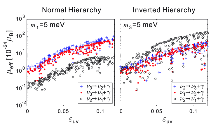
Figure 6: Illustration of the seesaw-induced non-unitary effects on $\mu_{\rm eff}$ for three active neutrinos. The standard (unitary) results correspond to $\varepsilon_{\rm uv}=0$, and their uncertainties come from the three unknown CP-violating phases of $X$.

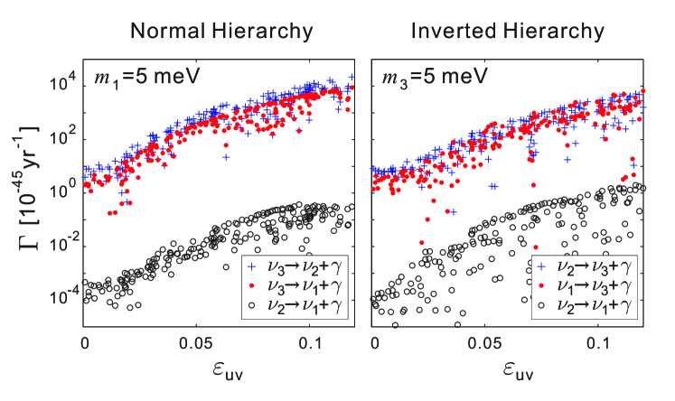
Figure 7: Illustration of the seesaw-induced non-unitary effects on $\Gamma_{\nu_{i}\to\nu_{j}+\gamma}$ for three active neutrinos. The standard (unitary) results correspond to $\varepsilon_{\rm uv}=0$, and their uncertainties come from the three unknown CP-violating phases of $X$.

6.2 Numerical Illustration

Figs. 6 and 7 illustrate the numerical results of the non-unitary effects on $\mu_{\rm eff}$ and $\Gamma_{\nu_{i}\to\nu_{j}+\gamma}$ respectively [141]. Note that in this numerical analysis those small active-sterile neutrino mixing angles in Eq. (59) are constrained by present experimental data [150] as follows:

$$T_{11}<5.5\times 10^{-3}\;,~{}~{}~{}~{}\left|T_{21}\right|<7.0\times 10^{-5}\;,$$

$$T_{22}<5.0\times 10^{-3}\;,~{}~{}~{}~{}\left|T_{31}\right|<1.6\times 10^{-2}\;,$$

$$T_{33}<5.0\times 10^{-3}\;,~{}~{}~{}~{}\left|T_{32}\right|<1.0\times 10^{-2}\;.$$ (62)

All $s_{ik}$ in $T$ (for $i=1,2,3$ and $k=4,5,6$) are positive or vanishing. The CP phases $\delta_{ik}$ are all allowed to vary from zero to $2\pi$, but they must satisfy the above constraints together with the relations $UU^{\dagger}+RR^{\dagger}={\bf 1}$ and $U\widehat{M}_{\nu}U^{T}+R\widehat{M}_{N}R^{T}={\bf 0}$. To assure that radiative corrections to the masses of three light neutrinos (via the one-loop self-energy diagrams involving the heavy neutrinos) are sufficiently small (e.g., smaller than $0.5$ meV) and stable, we simply assume that the masses of three heavy neutrinos are nearly degenerate [154, 155] and not more than ${\cal O}(1)$ TeV. This assumption implies that the results shown here are for a limited and safe parameter space of the TeV seesaw mechanism, but it is instructive enough to reveal the salient features of the non-unitary effects on the effective EMDMs $\mu_{\rm eff}(\nu_{i}\to\nu_{j}+\gamma)$ and the radiative decay rates $\Gamma_{\nu_{i}\to\nu_{j}+\gamma}$.

To present our numerical results in a convenient way, let us define

$$\varepsilon_{\rm uv}\equiv\left[\sum^{6}_{k=4}\left(s^{2}_{1k}+s^{2}_{2k}+s^{2}_{3k}\right)\right]^{1/2}\;,$$ (63)

which measures the overall strength of the unitarity violation of $U$, and $\varepsilon_{\rm uv}\in[0,0.15)$ is reasonably taken in our calculations. Namely, we allow each $s_{ik}$ (for $i=1,2,3$ and $k=4,5,6$) to vary in the range $0\leq s_{ik}<0.15$. The numerical dependence of $\mu_{\rm eff}(\nu_{i}\to\nu_{j}+\gamma)$ and $\Gamma_{\nu_{i}\to\nu_{j}+\gamma}$ on $\varepsilon_{\rm uv}$ is shown in Figs. 6 and 7, respectively. Some discussions are in order.

(1) Switching off the non-unitary effects (i.e., $\varepsilon_{\rm uv}=0$), we obtain the effective electromagnetic dipole moments

$$\mu_{\rm eff}\simeq\left\{\begin{array}[]{l}\left(0.8\sim 3.0\right)\times 10^{-25}~{}\mu_{\rm B}~{}~{}~{}~{}~{}~{}(\nu_{2}\to\nu_{1}+\gamma)\;,\\ \left(0.8\sim 1.5\right)\times 10^{-24}~{}\mu_{\rm B}~{}~{}~{}~{}~{}~{}(\nu_{3}\to\nu_{1}+\gamma)\;,\\ \left(1.1\sim 2.1\right)\times 10^{-24}~{}\mu_{\rm B}~{}~{}~{}~{}~{}~{}(\nu_{3}\to\nu_{2}+\gamma)\;,\end{array}\right.$$ (67)

for the normal mass hierarchy with $m_{1}\simeq 5$ meV; and

$$\mu_{\rm eff}\simeq\left\{\begin{array}[]{l}\left(0.01\sim 2.0\right)\times 10^{-24}~{}\mu_{\rm B}~{}~{}~{}~{}~{}(\nu_{2}\to\nu_{1}+\gamma)\;,\\ \left(0.8\sim 1.5\right)\times 10^{-24}~{}\mu_{\rm B}~{}~{}~{}~{}~{}~{}\;(\nu_{3}\to\nu_{1}+\gamma)\;,\\ \left(1.3\sim 2.0\right)\times 10^{-24}~{}\mu_{\rm B}~{}~{}~{}~{}~{}~{}\;(\nu_{3}\to\nu_{2}+\gamma)\;,\end{array}\right.$$ (71)

for the inverted mass hierarchy with $m_{3}\simeq 5$ meV, where the uncertainties mainly come from the unknown CP phases $\delta_{12}$, $\delta_{13}$ and $\delta_{23}$. Such standard (unitary) results are far below the observational upper bound on $\mu_{\rm eff}$ ($<$ a few $\times 10^{-11}~{}\mu_{\rm B}$ [152, 153]), but they serve as a good reference to the non-unitary effects on $\mu_{\rm eff}$ being explored.

(2) Figs. 6 and 7 clearly show that $\mu_{\rm eff}$ and $\Gamma_{\nu_{i}\to\nu_{j}+\gamma}$ can be maximally enhanced by a factor of ${\cal O}(10^{2})$ and a factor of ${\cal O}(10^{4})$, respectively, in particular when $\varepsilon_{\rm uv}$ approaches its upper limit as set by current experimental data. The magnitude of $\mu_{\rm eff}(\nu_{2}\to\nu_{1}+\gamma)$ may be strongly suppressed in the inverted neutrino mass hierarchy. The reason is rather simple: on the one hand, $m_{1}\simeq m_{2}$ holds in this case, and thus $\epsilon_{12}\propto(m_{2}-m_{1})$ must be very small; on the other hand, $\mu_{12}$ depends on ${\rm Im}(U_{\alpha 1}U^{*}_{\alpha 2})$, so it can also be very small when the CP-violating phases are around zero or $\pi$. This two-fold suppression becomes severer for the decay rate $\Gamma_{\nu_{2}\to\nu_{1}+\gamma}$, because it is proportional to $(m_{2}-m_{1})^{3}\mu^{2}_{\rm eff}(\nu_{2}\to\nu_{1}+\gamma)$.

(3) The results of $\mu_{\rm eff}$ and $\Gamma_{\nu_{i}\to\nu_{j}+\gamma}$ are sensitive to the absolute neutrino mass scale for both normal and inverted mass hierarchies. For instance, $\mu_{\rm eff}(\nu_{2}\to\nu_{1}+\gamma)$ and $\mu_{\rm eff}(\nu_{3}\to\nu_{1}+\gamma)$ get enhanced when $m_{1}$ changes from zero to 5 meV in the normal mass hierarchy; while $\mu_{\rm eff}(\nu_{1}\to\nu_{3}+\gamma)$ and $\mu_{\rm eff}(\nu_{2}\to\nu_{3}+\gamma)$ are enhanced when $m_{3}$ changes from zero to 5 meV in the inverted mass hierarchy. This kind of sensitivity is not so obvious if one only takes a look at the expressions of $\mu_{ij}$ and $\epsilon_{ij}$ in Eq. (57). The main reason is that a change of $m_{1}$ or $m_{3}$ requires some fine-tuning of the active-sterile neutrino mixing angles and CP-violating phases as dictated by the exact seesaw relation $U\widehat{M}_{\nu}U^{T}+R\widehat{M}_{N}R^{T}={\bf 0}$, leading to a possibly significant change of $\mu_{\rm eff}$. The dependence of $\Gamma_{\nu_{i}\to\nu_{j}+\gamma}$ on the absolute neutrino mass scale is somewhat more complicated, as one can see from Eq. (61).

(4) The CP-violating phases play a very important role in fitting both the exact seesaw relation and Eq. (62). If the heavy neutrino masses $M_{i}$ are not suppressed, then an appreciable value of $\varepsilon_{\rm uv}$ requires some fine cancellations in the matrix product $R\widehat{M}_{N}R^{T}$ such that sufficiently small $m_{i}$ can be obtained from $U\widehat{M}_{\nu}U^{T}=-R\widehat{M}_{N}R^{T}$. On the other hand, we remark that it is actually unnecessary to require $M_{i}$ to be around or above the electroweak scale. The seesaw-induced non-unitary effects on $\mu_{\rm eff}$ and $\Gamma_{\nu_{i}\to\nu_{j}+\gamma}$ can be significant even if one allows one, two or three heavy neutrinos to be relatively light (e.g., at the keV mass scale). Such sterile neutrinos are interesting in particle physics and cosmology. Note that it is easier to satisfy the exact seesaw relation with an appreciable value of $\varepsilon_{\rm uv}$ by arranging $M_{i}$ to lie in the keV, MeV or GeV range. This kind of low-scale seesaw scenarios [156] might be technically natural, but they have more or less lost the seesaw spirit. Of course, sufficiently large $M_{i}$ and sufficiently small $\theta_{ik}$ can always coexist to make the seesaw mechanism work in a natural way, but in this traditional case the non-unitary effects are too small to have any measurable consequences at low energies.

It is also worth pointing out that the seesaw-induced non-unitary effects on $\mu_{ij}$ and $\epsilon_{ij}$ are rather different from the case of making a naive assumption of the flavor mixing between three active neutrinos and a few light sterile neutrinos [39]. The latter can directly break the unitarity of the $3\times 3$ MNSP matrix $U$ and then lift the GIM suppression [151] associated with $\mu_{ij}$ and $\epsilon_{ij}$. This kind of non-unitary effects are not constrained by the seesaw relation, and thus they are more arbitrary and less motivated from the point of view of model building.

The effective electromagnetic dipole moments of three neutrinos and the rates of their radiative decays can be maximally enhanced by a factor of ${\cal O}(10^{2})$ and a factor of ${\cal O}(10^{4})$, respectively, no matter whether the seesaw scale is around or below the TeV energy scale. This observation is new and nontrivial, and it reveals an intrinsic and presumably important correlation between the electromagnetic properties of neutrinos and the origin of their masses. Such a correlation may even serve as a sensitive touch-stone for the highly-regarded seesaw mechanism.

7 SUMMARY

After the Daya Bay measurement of the smallest neutrino mixing angle $\theta_{13}$, it is natural to ask where we are standing and where we are expecting to go in neutrino physics. We have tried to answer these two questions from a phenomenological point of view in this review paper, although our answers are incomplete and full of conjectures. To be specific, we have given a fast overview of some fundamental neutrino properties and paid particular interest to the flavor issues of charged leptons and neutrinos, including the mass spectrum, flavor mixing pattern and CP violation. We have gone into details of possible lepton flavor structures by describing two useful phenomenological strategies and giving a number of typical examples. The impact of large $\theta_{13}$ on the running behaviors of other flavor mixing parameters has been discussed in the framework of the MSSM. We have also illustrated the seesaw-enhanced electromagnetic dipole moments of three Majorana neutrinos based on a viable TeV seesaw scenario.

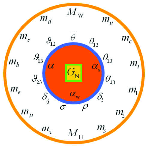
Figure 8: The Fritzsch-Xing plot for 29 fundamental parameters in Nature, describing four kinds of interactions ($G_{\rm N}$, $\alpha$, $\alpha_{\rm w}$ and $\alpha_{\rm s}$), six quark masses ($m_{u}$, $m_{c}$, $m_{t}$ and $m_{d}$, $m_{s}$, $m_{b}$), six lepton masses ($m_{e}$, $m_{\mu}$, $m_{\tau}$ and $m_{1}$, $m_{2}$, $m_{3}$), three quark flavor mixing angles ($\vartheta_{12}$, $\vartheta_{13}$ and $\vartheta_{23}$), three lepton flavor mixing angles ($\theta_{12}$, $\theta_{13}$ and $\theta_{23}$), two CP-violating phases in the quark sector ($\delta_{q}$ and $\overline{\theta}$), three CP-violating phases in the lepton sector ($\delta_{l}$, $\rho$ and $\sigma$), the Higgs mass $M_{\rm H}$ and the $W$-boson mass $M_{\rm W}$.

If only the SM particles are taken into account and the massive neutrinos are assumed to be the Majorana particles, we are then left with 29 fundamental parameters in Nature, as described by the so-called Fritzsch-Xing plot in Fig. 8. The determination of $\theta_{13}$ and $M_{\rm H}$ in 2012 is a milestone in particle physics. But the effective strong CP-violating phase $\overline{\delta}$ in the quark sector and the three weak CP-violating phases (i.e., $\delta_{l}$, $\rho$ and $\sigma$) in the lepton sector remain unknown. Moreover, the absolute mass scale of three neutrinos and their mass ordering have not been determined. We hope that various precision neutrino experiments can help pin down the relevant parameters in the lepton sector and then shed light on the flavor dynamics in the foreseeable future.

Of course, the picture in Fig. 8 may be too simple and too naive because we are not sure whether some of those “fundamental” parameters are really fundamental or not. New degrees of freedom, such as the sterile neutrinos or the supersymmetric particles, might be discovered and make the flavor sector much messier. If the underlying flavor theory is regarded as an animal, one has no idea whether it is a donkey or an elephant or something else. In this sense we are blind today and have to make a lot of experimental and theoretical efforts to identify its nose, eyes, ears, legs and so on in order to make sure what animal it is. The road behind has repeatedly told us that the road ahead is always challenging, but it is always exciting.

This review paper is essentially based on the plenary talk given by one of us (Z.Z.X.) at the SUSY 2012 conference. The work of S.L. is supported in part by the National Basic Research Program (973 Program) of China under Grant No. 2009CB824800, the National Natural Science Foundation of China under Grant No. 11105113 and the Fujian Provincial Natural Science Foundation under Grant No. 2011J05012. The work of Z.Z.X. is supported in part by the National Natural Science Foundation of China under grant No. 11135009.

References

- [1] F.P. An et al. (Baya Bay Collaboration), Phys. Rev. Lett. 108, 171803 (2012).
- [2] K. Abe et al. (T2K Collaboration), Phys. Rev. Lett. 107, 041801 (2011).
- [3] P. Adamson et al. (MINOS Collaboration), Phys. Rev. Lett. 107, 181802 (2011).
- [4] Y. Abe et al. (Double Chooz Collaboration), Phys. Rev. Lett. 108, 131801 (2012).
- [5] G. Aad et al. (ATLAS Collaboration), Phys. Lett. B 716, 1 (2012).
- [6] S. Chatrchyan et al. (CMS Collaboration), Phys. Lett. B 716, 30 (2012).
- [7] A. Einstein, Ann. Phys. 17, 891 (1905).
- [8] G. Feinberg, Phys. Rev. 159, 1089 (1967).
- [9] T. Adam et al. (OPERA Collaboration), arXiv:1109.4897 [hep-ex].
- [10] J. Alspector et al., Phys. Rev. Lett. 36, 837 (1976).
- [11] G.R. Kalbfleisch et al., Phys. Rev. Lett. 43, 1361 (1979).
- [12] P. Adamson et al. (MINOS Collaboration), Phys. Rev. D 76, 072005 (2007).
- [13] M. Antonello et al. (ICARUS Collaboration), Phys. Lett. B 713, 17 (2012).
- [14] M. Antonello et al., arXiv:1208.2629 [hep-ex].
- [15] P. Alvarez Sanchez et al. (Borexino Collaboration), Phys. Lett. B 716, 401 (2012).
- [16] N.Y. Agafonova et al. (LVD Collaboration), Phys. Rev. Lett. 109, 070801 (2012).
- [17] K. Hirata et al. (Kamiokande II Collaboration), Phys. Rev. Lett. 58, 1490 (1987).
- [18] M.J. Longo, Phys. Rev. D 36, 3276 (1987).
- [19] L. Stodolsky, Phys. Lett. B 201, 353 (1988).
- [20] P. Minkowski, Phys. Lett. B 67, 421 (1977).
- [21] T. Yanagida, in Proceedings of the Workshop on Unified Theory and the Baryon Number of the Universe, edited by O. Sawada and A. Sugamoto (KEK, Tsukuba, 1979), p. 95.
- [22] M. Gell-Mann, P. Ramond, and R. Slansky, in Supergravity, edited by P. van Nieuwenhuizen and D. Freedman (North Holland, Amsterdam, 1979), p. 315.
- [23] S.L. Glashow, in Quarks and Leptons, edited by M. Lvy et al. (Plenum, New York, 1980), p. 707.
- [24] R.N. Mohapatra and G. Senjanovic, Phys. Rev. Lett. 44, 912 (1980).
- [25] S. Dodelson and L.M. Widrow, Phys. Rev. Lett. 72, 17 (1994).
- [26] X.D. Shi and G.M. Fuller, Phys. Rev. Lett. 82, 2832 (1999)
- [27] A.D. Dolgov and S.H. Hansen, Astropart. Phys. 16, 339 (2002).
- [28] F. Bezrukov, H. Hettmansperger, and M. Lindner, Phys. Rev. D 81, 085032 (2010).
- [29] W. Liao, Phys. Rev. D 82, 073001 (2010).
- [30] Y.F. Li and Z.Z. Xing, Phys. Lett. B 695, 205 (2011).
- [31] M. Nemevsek, G. Senjanovic and Y. Zhang, JCAP 1207, 006 (2012).
- [32] Z.Z. Xing, Phys. Rev. D 68, 053002 (2003).
- [33] Z.Z. Xing, Int. J. Mod. Phys. A 19, 1 (2004).
- [34] W. Rodejohann, Int. J. Mod. Phys. E 20, 1833 (2011).
- [35] W. Rodejohann, arXiv:1206.2560 [hep-ph].
- [36] B.W. Lee and R. Shrock, Phys. Rev. D 16, 1444 (1977).
- [37] K. Fujikawa and R. Shrock, Phys. Rev. Lett. 45, 963 (1980).
- [38] A. Strumia and F. Vissani, hep-ph/0606054.
- [39] K.N. Abazajian et al., arXiv:1204.5379 [hep-ph].
- [40] M. Fukugita and T. Yanagida, Phys. Lett. B 174, 45 (1986).
- [41] A. Aguilar et al. (LSND Collaboration), Phys. Rev. D 64, 112007 (2001).
- [42] A.A. Aguilar-Arevalo et al. (MiniBooNE Collaboration), Phys. Rev. Lett. 105, 181801 (2010).
- [43] G. Mention et al., Phys. Rev. D 83, 073006 (2011).
- [44] J. Kopp, M. Maltoni, and T. Schwetz, Phys. Rev. Lett. 107, 091801 (2011).
- [45] C. Giunti and M. Laveder, Phys. Rev. D 84, 073008 (2011).
- [46] See, e.g., G. Mangano and P.D. Serpico, Phys. Lett. B 701, 296 (2011); and references therein.
- [47] J. Hamann et al., Phys. Rev. Lett. 105, 181301 (2010).
- [48] J. Hamann et al., JCAP 1109, 034 (2011).
- [49] E. Giusarma et al., Phys. Rev. D 83, 115023 (2011).
- [50] P. Bode, J.P. Ostriker, and N. Turok, Astrophys. J. 556, 93 (2001).
- [51] Z.Z. Xing, Phys. Rev. D 85, 013008 (2012).
- [52] Z. Maki, M. Nakagawa, and S. Sakata, Prog. Theor. Phys. 28, 870 (1962).
- [53] B. Pontecorvo, Sov. Phys. JETP 26, 984 (1968).
- [54] J. Beringer et al. (Particle Data Group), Phys. Rev. D 86, 010001 (2012).
- [55] G.L. Fogli et al., Phys. Rev. D 86, 013012 (2012).
- [56] M.C. Gonzalez-Garcia and M. Maltoni, Phys. Rept. 460, 1 (2008); and references therein.
- [57] S. Choubey, S.T. Petcov, and M. Piai, Phys. Rev. D 68, 113006 (2003).
- [58] L. Zhan, Y. Wang, J. Cao and L. Wen, Phys. Rev. D 78, 111103 (2008).
- [59] P.H. Frampton, S.L. Glashow, and T. Yanagida, Phys. Lett. B 548, 119 (2002).
- [60] For a review, see: W.L. Guo, Z.Z. Xing, and S. Zhou, Int. J. Mod. Phys. E 16, 1 (2007).
- [61] R. Friedberg and T.D. Lee, High Energy Phys. Nucl. Phys. 30, 591 (2006).
- [62] Z.Z. Xing, H. Zhang, and S. Zhou, Phys. Lett. B 641, 189 (2006).
- [63] S. Luo and Z.Z. Xing, Phys. Lett. B 646, 242 (2007).
- [64] Z.Z. Xing, Int. J. Mod. Phys. E 16, 1361 (2007).
- [65] C. Jarlskog, Phys. Rev. D 77, 073002 (2008).
- [66] C.S. Huang, T.J. Li, W. Liao, and S.H. Zhu, Phys. Rev. D 78, 013005 (2008).
- [67] S. Luo, Z.Z. Xing, and X. Li, Phys. Rev. D 78, 117301 (2008).
- [68] Z.Z. Xing and S. Zhou, Phys. Lett. B 666, 166 (2008).
- [69] C. Jarlskog, Phys. Rev. Lett. 55, 1039 (1985).
- [70] Z.Z. Xing, Nuovo Cim. A 109, 115 (1996)
- [71] Z.Z. Xing, J. Phys. G 23, 717 (1997).
- [72] Z.Z. Xing, arXiv:1210.1523 [hep-ph].
- [73] H. Fritzsch and Z.Z. Xing, Prog. Part. Nucl. Phys. 45, 1 (2000); and references therein.
- [74] Z.Z. Xing, Chin. Phys. C 36, 281 (2012).
- [75] H. Fritzsch and Z.Z. Xing, Phys. Rev. D 61, 073016 (2000).
- [76] Z.Z. Xing, H. Zhang, and S. Zhou, Phys. Rev. D 77, 113016 (2008).
- [77] Z.Z. Xing, H. Zhang, and S. Zhou, Phys. Rev. D 86, 013013 (2012).
- [78] H. Fritzsch and Z.Z. Xing, Phys. Lett. B 634, 514 (2006).
- [79] H. Fritzsch and Z.Z. Xing, Phys. Lett. B 682, 220 (2009).
- [80] H. Fritzsch, Phys. Lett. B 73, 317 (1978).
- [81] H. Fritzsch, Nucl. Phys. B 155, 189 (1979).
- [82] Z.Z. Xing, Phys. Lett. B 550, 178 (2002).
- [83] S. Zhou and Z.Z. Xing, Eur. Phys. J. C 38, 495 (2005);
- [84] H. Fritzsch, Z.Z. Xing, Y.L. Zhou, Phys. Lett. B 697, 357 (2011).
- [85] Z.Z. Xing, Phys. Lett. B 530, 159 (2002).
- [86] P.H. Frampton, S.L. Glashow, and D. Marfatia, Phys. Lett. B 536, 79 (2002).
- [87] Z.Z. Xing, Phys. Lett. B 539, 85 (2002).
- [88] For a systematic analysis, see: H. Fritzsch, Z.Z. Xing, and S. Zhou, JHEP 1109, 083 (2011).
- [89] C.D. Froggatt and H.B. Nielsen, Nucl. Phys. B 147, 277 (1979).
- [90] See, e.g., W. Grimus, A.S. Joshipura, L. Lavoura, and M. Tanimoto, Eur. Phys. J. C 36, 227 (2004).
- [91] H. Fritzsch and Z.Z. Xing, Phys. Lett. B 372, 265 (1996).
- [92] H. Fritzsch and Z.Z. Xing, Phys. Lett. B 440, 313 (1998).
- [93] G. Altarelli and F. Feruglio, Rev. Mod. Phys. 82, 2701 (2010).
- [94] L. Merlo, arXiv:1004.2211 [hep-ph].
- [95] F. Vissani, hep-ph/9708483.
- [96] V. Barger, S. Pakvasa, T.J. Weiler, and K. Whisnant, Phys. Lett. B 437, 107 (1998).
- [97] P.F. Harrison, D.H. Perkins, and W.G. Scott, Phys. Lett. B 530, 167 (2002).
- [98] Z.Z. Xing, Phys. Lett. B 533, 85 (2002).
- [99] P.F. Harrison and W.G. Scott, Phys. Lett. B 535, 163 (2002).
- [100] X.G. He and A. Zee, Phys. Lett. B 560, 87 (2003).
- [101] Y. Kajiyama, M. Raidal, and A. Strumia, Phys. Rev. D 76, 117301 (2007).
- [102] A slight variation of this golden-ratio mixing pattern has been discussed by W. Rodejohann, Phys. Lett. B 671, 267 (2009).
- [103] Z.Z. Xing, J. Phys. G 29, 2227 (2003).
- [104] C. Giunti, Nucl. Phys. B (Proc. Suppl.) 117, 24 (2003).
- [105] The name of this flavor mixing pattern was coined by C.H. Albright, A. Dueck, and W. Rodejohann, Eur. Phys. J. C 70, 1099 (2010).
- [106] Z.Z. Xing, Phys. Lett. B 696, 232 (2011).
- [107] W. Rodejohann, H. Zhang, and S. Zhou, Nucl. Phys. B 855, 592 (2012).
- [108] R. de Adelhart Toorop, F. Feruglio, and C. Hagedorn, Nucl. Phys. B 858, 437 (2012).
- [109] Z.Z. Xing, Phys. Rev. D 78, 011301 (2008).
- [110] S. Antusch, J. Kersten, M. Lindner, and M. Ratz, Phys. Lett. B 544, 1 (2002).
- [111] S. Antusch and M. Ratz, JHEP 0211, 010 (2002).
- [112] J.W. Mei and Z.Z. Xing, Phys. Rev. D 70, 053002 (2004).
- [113] J.W. Mei and Z.Z. Xing, Phys. Lett. B 623, 227 (2005).
- [114] J.W. Mei, Phys. Rev. D 71, 073012 (2005).
- [115] S. Luo and Z.Z. Xing, Phys. Lett. B 632, 341 (2006).
- [116] S. Luo and Z.Z. Xing, Phys. Lett. B 637, 279 (2006).
- [117] S. Goswami, S.T. Petcov, S. Ray, and W. Rodejohann, Phys. Rev. D 80, 053013 (2009).
- [118] T. Araki, C.Q. Geng, and Z.Z. Xing, Phys. Lett. B 699, 276 (2011).
- [119] T. Araki and C.Q. Geng, JHEP 1109, 139 (2011).
- [120] H. Zhang and S. Zhou, Phys. Lett. B 704, 296 (2011).
- [121] S. Luo and Z.Z. Xing, arXiv:1203.3118 [hep-ph].
- [122] Z.Z. Xing and S. Zhou, Phys. Lett. B 653, 278 (2007).
- [123] S. Zhou, arXiv:1205.0761 [hep-ph].
- [124] Z.Z. Xing, Chin. Phys. C 36, 101 (2012).
- [125] P.H. Chankowski and Z. Pluciennik, Phys. Lett. B 316, 312 (1993).
- [126] K.S. Babu, C.N. Leung, and J.T. Pantaleone, Phys. Lett. B 319, 191 (1993).
- [127] N. Haba, N. Okamura, and M. Sugiura, Prog. Theor. Phys. 103, 367 (2000).
- [128] S. Antusch et al., Phys. Lett. B 519, 238 (2001).
- [129] S. Antusch et al., Phys. Lett. B 525, 130 (2002).
- [130] S. Antusch, J. Kersten, M. Lindner, and M. Ratz, Nucl. Phys. B 674, 401 (2003).
- [131] S. Antusch et al., JHEP 0503, 024 (2005).
- [132] M. Lindner, M. Ratz, and M. A. Schmidt, JHEP 0509, 081 (2005).
- [133] Z.Z. Xing, Phys. Lett. B 633, 550 (2006).
- [134] Z.Z. Xing and H. Zhang, Commun. Theor. Phys. 48, 525 (2007).
- [135] S. Weinberg, Phys. Rev. Lett. 43, 1566 (1979).
- [136] S. Luo, J.W. Mei, and Z.Z. Xing, Phys. Rev. D 72, 053014 (2005).
- [137] For a brief review, see: Z.Z. Xing, Prog. Theor. Phys. Suppl. 180, 112 (2009); and references therein.
- [138] V. Tello, M. Nemevsek, F. Nesti, G. Senjanovic and F. Vissani, Phys. Rev. Lett. 106, 151801 (2011).
- [139] M. Nemevsek, F. Nesti, G. Senjanovic and V. Tello, arXiv:1112.3061 [hep-ph].
- [140] M. Nemevsek, G. Senjanovic and V. Tello, arXiv:1211.2837 [hep-ph].
- [141] Z.Z. Xing and Y.L. Zhou, Phys. Lett. B 715, 178 (2012).
- [142] See, e.g., A. Mirizzi, D. Montanino, and P. Serpico, Phys. Rev. D 76, 053007 (2007).
- [143] S. Matsuura et al., Astrophys. J. 737, 2 (2011).
- [144] S.H. Kim et al., J. Phys. Soc. Jap. 81, 024101 (2012).
- [145] Z.Z. Xing, Phys. Lett. B 660, 515 (2008).
- [146] R.E. Shrock, Nucl. Phys. B 206, 359 (1982).
- [147] P.B. Pal and L. Wolfenstein, Phys. Rev. D 25, 766 (1982).
- [148] B. Kayser, Phys. Rev. D 26, 1662 (1982).
- [149] J.F. Nieves, Phys. Rev. D 26, 3152 (1982).
- [150] S. Antusch et al., JHEP 0610, 084 (2006).
- [151] S.L. Glashow, J. Iliopoulos, and L. Maiani, Phys. Rev. D 2, 1285 (1970).
- [152] G.G. Raffelt, Phys. Rept. 320, 319 (1999).
- [153] C. Giunti and A. Studenikin, Phys. Atom. Nucl. 72, 2089 (2009).
- [154] A. Pilaftsis, Z. Phys. C 55, 275 (1992).
- [155] S. Zhou, PhD Thesis (Institute of High Energy Physics, Beijing, 2009).
- [156] A. de Gouvea, J. Jenkins, and N. Vasudevan, Phys. Rev. D 75, 013003 (2007).