On Achievable Schemes of Interference Alignment in Constant Channels via Finite Amplify-and-Forward Relays

Abstract

This paper elaborates on the achievable schemes of interference alignment in constant channels via finite amplify-and-forward (AF) relays. Consider $K$ sources communicating with $K$ destinations without direct links besides the relay connections. The total number of relays is finite. The objective is to achieve interference alignment for all user pairs to obtain half of their interference-free degrees of freedom. In general, two strategies are employed: coding at the edge and coding in the middle, in which relays show different roles. The contributions are that two fundamental and critical elements are captured to enable interference alignment in this network: channel randomness or relativity; subspace dimension suppression.

I Introduction

Since interference alignment (IA) is a new multiplexing gain maximizing technique [1] and relay is considered a cost-effective solution for coverage extension and capacity enhancement, recently many researchers have been investigating schemes to combine these two techniques [2, 3]. Various scenarios have been intensively studied, e.g. decode-and-forward relays [4, 5], multi-user broadcast channel [6], clustered relays [7], two-way relay selection [8]. Among all the scenarios, the model of multi-user peer-peer two-hop interference channel with amplify-and-forward relays without direct links has received increasing attention due to its wide application in practice [9, 10, 11, 12], which show that relays help the system to obtain higher degrees of freedom (DoF) in high signal-to-noise ratio (SNR) regime.

While peer-peer multi-user interference channel has been traditionally regarded as a challenging scenario due to channel inseparability [13], not to mention with relays in between. Furthermore, current relay networks are categorized into two main sets: one is that relays are auxiliary links in addition to direct links between both ends [2, 14, 15, 16, 17]; the other is that relays are the only connection path for end nodes without direct links [3]. In general, relay networks with direct links are well structured to construct IA. However, this work considers relay networks without direct links where relay generated equivalent channels are quite complicated and poorly structured [3, 18, 19]. In that case, many approaches are proposed, e.g. [3] requires an infinite number of relays to eliminate interference; [18] exploits ergodic nature in fading channels; [19] illustrates interference neutralization in a special $2\times 2\times 2$ network; [9] uses mean squared error (MSE) numerical method to minimize interference.

Three important features are highlighted in the scenario of this work: the number of relays is finite so that it is impossible to have the unpractical solution in [3] to eliminate interference with infinite number of relays; each node could only have single antenna to achieve IA; time-invariant channels are also available to achieve IA even with single antenna nodes [1]. This work borrows the two strategies generalized in multiple unicast problem [20], which are coding at the edge and coding in the middle. In the first strategy of coding at the edge, relays randomly construct equivalent channels while end nodes proceed with conventional interference alignment schemes. Compared with other research, the most unfavorable conditions are set in this work: all end and relay nodes are single antenna; all channels are time-invariant; relay number is set to be finite, e.g one or two. Max-flow-min-cut theorem is not directly applicable in this scenario. In the second strategy of coding in the middle, optimization techniques are applied to numerically approach interference alignment with all nodes set to be multi-antenna.

Our contributions are in two folds:

A new fact is unveiled that when the network has only one relay, Cadambe-Jafar scheme is not applicable in signal vector alignment; Motahari-Khandani scheme is not applicable in signal level alignment; asymmetric complex signaling is not applicable in phase alignment. The reason is that relay-emulated channels lose randomness or relativity. Then the problem is settled by two ways. On one hand, at least two relays are necessary to emulate qualified channels to generate randomness. On the other hand, to generate randomness still in the one-relay channel, space-time type of precoding methods are applicable at the edge; the conceptual idea of blind interference alignment is also applicable to fluctuate channels with the only one relay. By all these analysis and schemes, a novel unique role of relays in the network is revealed to overcome the channel randomness issue.

A novel solution is proposed for IA via relay coding based on a non-trivial application of existing rank constrained rank minimization (RCRM) method [21, 22]. Conventional optimization and numerical algorithms are non-convex or hard for interference alignment [23, 9, 5]. Since RCRM method is originally not for relay networks, the convexity is proved for the new application. This novel solution has three advantages: a) it considers DoF at high SNR by subspace dimension minimization while other numerical methods could only consider sum rate and mean squared error (MSE); b) it is universal to be conveniently applied to a number of scenarios, e.g. MIMO amplify-and-forward(AF) relay channel, MIMO two-way AF relay channel, MIMO Y channel, and MIMO multi-hop relay channel. c) actually conventional analytical and numerical solutions are hard to obtain for the mentioned scenarios, while this novel method accomplishes the design and is robust to poor conditions. Numerical results show its effectiveness.

II Problem Statement and Model Description

II-A Basic Model

Consider $K$ sources and $K$ destinations connected by $L$ relays as shown in Fig. 1. Direct links between end users are not available. All nodes are single antenna, denote the channel from source $i$ to relay $l$ as $\mathrm{h}_{li}$ and the channel from relay $l$ to destination $j$ as $\mathrm{f}_{jl}$. Denote the sets $\mathcal{K}=\{1,2,\ldots,K\}$, $\mathcal{L}=\{1,2,\ldots,L\}$, so that $i,j\in\mathcal{K}$, $l\in\mathcal{L}$. All channels are quasi-static, i.e. $\mathrm{h}_{li}$ and $\mathrm{f}_{jl}$ are scalar constants.

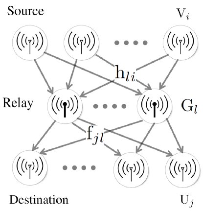
Figure 1: Basic model of sources, relays, and destinations

Time-extended MIMO scheme in [3] is used so that $T$ consecutive symbols form one signal and the relay coding matrix at $l$-th relay is

$$\mathrm{G}_{l}=\Big{[}\mathrm{g}_{l}(p,q)\Big{]}_{T\times T}$$ (1)

in which $\mathrm{g}_{l}(p,q)$ is the relay gain from the $q$-th time slot to the $p$-the time slot at the $l$-th relay. Then the received signal at $j$-th user can be written as

$$\mathrm{Y}_{j} =\Theta_{jj}\mathrm{V}_{j}\mathrm{X}_{j}+\sum_{i=1,i\neq j}^{K}\Theta_{ji}\mathrm{V}_{i}\mathrm{X}_{i}+\mathrm{Z}_{j}$$ (2)

$$\Theta_{ji}=\sum_{l=1}^{L}\mathrm{f}_{jl}\mathrm{G}_{l}\mathrm{h}_{li}$$ (3)

where $\mathrm{X}_{i}\in\mathbb{C}^{d\times 1}$ is the $d$ input streams at $i$-th source and $\mathrm{V}_{i}\in\mathbb{C}^{T\times d}$ is precoding matrix. $\mathrm{Z}_{j}\in\mathbb{C}^{T\times 1}$ is the noise at $j$-th receiver, and $\mathrm{Y}_{j}\in\mathbb{C}^{T\times 1}$. The equivalent channel matrix from the $i$-th source to the $j$-th destination is defined as $\Theta_{ji}$ for simplicity. The holistic system equation is also written as:

$$\left[\begin{aligned} &\mathrm{Y}_{1}\\ &\mathrm{Y}_{2}\\ &\ \ \vdots\\ &\mathrm{Y}_{K}\end{aligned}\right]=\sum_{l=1}^{L}\left[\begin{aligned} &\mathrm{f}_{1l}\mathrm{h}_{l1}\mathrm{G}_{l}\cdots\mathrm{f}_{1l}\mathrm{h}_{lK}\mathrm{G}_{l}\\ &\mathrm{f}_{2l}\mathrm{h}_{l1}\mathrm{G}_{l}\cdots\mathrm{f}_{2l}\mathrm{h}_{lK}\mathrm{G}_{l}\\ &\ \ \ \ddots\ \ \ \mathrm{f}_{jl}\mathrm{h}_{li}\mathrm{G}_{l}\ \ \ddots\\ &\mathrm{f}_{Kl}\mathrm{h}_{l1}\mathrm{G}_{l}\cdots\mathrm{f}_{Kl}\mathrm{h}_{lK}\mathrm{G}_{l}\end{aligned}\right]\left[\begin{aligned} &\mathrm{V}_{1}\mathrm{X}_{1}\\ &\mathrm{V}_{2}\mathrm{X}_{2}\\ &\ \ \ \vdots\\ &\mathrm{V}_{K}\mathrm{X}_{K}\end{aligned}\right]+\left[\begin{aligned} &\mathrm{Z}_{1}\\ &\mathrm{Z}_{2}\\ &\ \ \vdots\\ &\mathrm{Z}_{K}\end{aligned}\right]$$ (4)

II-B General Model

For more general cases, the model is illustrated in Fig. 2. Denote $K$ nodes on one end as ${I}_{1},{I}_{2},\cdots,{I}_{K}$; $L$ relay nodes in the middle as ${R}_{1},{R}_{2},\cdots,{R}_{L}$; $K$ nodes on the other end as ${J}_{1},\cdots,{J}_{K-1},{J}_{K}$. Define sets $\mathcal{K}=\{1,2,\ldots,K\}$, $\mathcal{L}=\{1,2,\ldots,L\}$. All channels are time-invariant. Assume all nodes have all channel knowledge to cooperate.

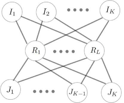
Figure 2: General model of sources, relays, destinations

In the case when all nodes are single antenna, denote $\mathrm{h}_{R_{l}I_{i}}$, $\mathrm{h}_{J_{j}R_{l}}$, as channels from $I_{i}$ to $R_{l}$, $R_{l}$ to $J_{j}$, respectively, where $i,j\in\mathcal{K}$, $l\in\mathcal{L}$, all channel coefficients are scalars. While in the case when all nodes are multiple antenna, denote $\mathrm{H}_{R_{l}I_{i}}$, $\mathrm{H}_{I_{i}R_{l}}$, $\mathrm{H}_{J_{j}R_{l}}$, $\mathrm{H}_{R_{l}J_{j}}$, as channels from $I_{i}$ to $R_{l}$, $R_{l}$ to $I_{i}$, $R_{l}$ to $J_{j}$, $J_{j}$ to $R_{l}$, respectively, where $i,j\in\mathcal{K}$, $l\in\mathcal{L}$, all channel coefficients are matrices.

III Characteristics of Amplify-and-Forward and Finite Relays

Before detailed design and analysis, this relay scenario needs to be characterized and some critical features should be exposed. First, the applicability of max-flow-min-cut theorem in this network is actually in doubt along with the amplify-and-forward scheme. Second, the number of relays, achievable DoF, and coding strategy are correlated in a complicated form.

III-A Amplify-and-Forward Scheme and Max-Flow-Min-Cut Theorem

A natural question arises here: Does max-flow-min-cut theorem still work in this IA relay network? Another similar question is: in a $K$-pair network with finite relays, what does the achievable DoF equal to? The answers to these two questions are quite nuanced actually.

Look into the $K$-pair network with $L$ relays. The first hop is a $K\times L$ MIMO link and the second hop is a $L\times K$ MIMO link. Conventionally, both the first and the second channel matrices only have a rank of $L$, which means that for the whole $K$-pair network, the minimum cut is $L$. However, the degrees of freedom for the network is not necessarily $L$. Consider the $K$-pair network regardless of the middle connections, so that there are potentially $K$ DoF for this equivalent network as long as with joint processing across the $K$ transmitters or receivers. The critical difference is that the intermediate relay nodes do not necessarily process data flows directly, and could act only as equivalent channels. In addition, instead of joint processing, a distributed manner such as interference alignment could still possibly achieve $K/2$ DoF. However, it is also important to highlight that when there are finite single-antenna relays, the equivalent channel may be rank deficient, which is discussed detailedly in the following parts.

DoF as in the signal processing model is not simply equal to capacity flow links as in network coding model. In the flow network model, each node has separate inputs and outputs, and each edge represents a separate link. While in amplify-and-forward relay networks, arbitrary flows could overlap through same relays, and links in each hop does not represent separate flows.Max-flow min-cut theorem is originally applied to wired networks with single-letter characterizations. A recent model for wireless relay networks is known as the linear deterministic relay network model with a max-flow min-cut result pertaining to it [24]. The algorithmic framework is introduced by Avestimehr, Diggavi and Tse, incorporating the key features of broadcasting and superposition. The signals are elements of a finite field and the interactions between the signals are assumed to be linear. This model is based on linking systems and the max-flow min-cut theorem is applicable with matroid intersection or partition.

Moreover, [20] shows that in a network with 3 unicast sessions each with min-cut of 1, whenever network alignment can achieve rate of 1/2 per session, there exists an alternative approach including routing, packing butterflies, random linear network coding, or other network coding strategies instead of alignment. However when there are more than 3 sessions, alignment is required to obtain the maximum rate as 1/2 the min-cut, while no other method can achieve it.

In summary, the max-flow min-cut theorem is not exactly available for this amplify-and-forward system, and DoF is not determined directly based on the number of relays. So that it is non-trivial to investigate new schemes in the amplify-and-forward strategy. Before further understanding and analyzing the DoF of this network, different situations need to be classified as following.

III-B Finite/Infinite Relays, DoF Limits, and Strategies

For the $K$-pair amplify-and-forward relay network, all the cases are roughly classified into three categories: when infinite relays are provided, full $K$ DoF is achievable, by using relay coding; when finite relays are provided, only fractional DoF is achievable as the number of users $K$ grows, by using conventional MIMO precoding approach; when a specific range of finite relays are provided, $K/2$ DoF is possible to be obtained, by using asymptotic interference alignment precoding approach. The details are shown in Table I and discussed as following.

Case	Relay Number	Target DoF	Coding	Channel	IA Scheme
1	Infinite	$K$	Relay Coding	Generic	N/A
2	Finite	$\frac{2}{K+1}$	Precoding	$\begin{aligned} &\ \ \text{Generic}\\ &\text{or Diagonal}\end{aligned}$	$\begin{aligned} &\ \ \ \text{Leakage}\\ &\text{Minimization}\end{aligned}$
3	$\begin{aligned} &\text{Specific}\\ &\text{Finite}\end{aligned}$	$K/2$	Precoding	Diagonal	Asymptotic

TABLE I: Classifications according to relay number, DoF Limits, and Strategies

III-B1 Infinite Relays, Full DoF, and Relay Coding

Consider the single antenna $K$-pair relay network in Fig. 1 with the system equation of (2) and the equivalent channel in (3). Let the interference at any receiver to be zero, and then the condition for $j$-th user should satisfy the following:

$$\ \ \ \ \ \ \mathrm{\Theta}_{ji}=\mathbf{0}\ \ \ \ \forall i\neq j$$ (5)

$$\text{i.e.}\ \ \sum_{l=1}^{L}\mathrm{f}_{jl}\mathrm{G}_{l}\mathrm{h}_{li}=\mathbf{0}\ \ \ \forall i\neq j$$

Equation (5) represents $K(K-1)$ matrix equations, equalling to $T^{2}K(K-1)$ linear equations. The matrices $\mathrm{G}_{1},\mathrm{G}_{2},\cdots,\mathrm{G}_{L}$ contain $LT^{2}$ variables. Generally, the equations are solvable when: $LT^{2}\geq T^{2}K(K-1)$, i.e. $L\geq K(K-1)$. It could be also interpreted as for each set of $L$ elements of $\{\mathrm{G}_{1}(l_{1},l_{2}),\mathrm{G}_{2}(l_{1},l_{2}),\cdots,\mathrm{G}_{L}(l_{1},l_{2})\}$ there are $K(K-1)$ equations. Therefore in this case, the network achieves $K$ DoF by only using the linear relay coding.

III-B2 Finite Relays, Fractional DoF, and Precoding

Consider the same network in Fig. 1. However, there’re only finite relays in this case. Instead of relay coding as above, a scheme of precoding on the equivalent channels is proposed, i.e. following the coding at the edge strategy [20]. Relays generate equivalent channels, and the $K$ transmitters and $K$ receivers only see the equivalent channels regardless of relays. Then conventional interference alignment methods could be used directly for all $K$ users [1], [23].

The relay gain matrices of (1) are randomly chosen to be in a generic form (full elements), so that $\mathrm{G}_{l}$ and corresponding $\mathrm{\Theta}_{ji}$ are equivalent to general MIMO channels. The leakage minimization algorithm of [23] is applicable to approach interference alignment. However, according to the feasibility condition in [25] for symmetric MIMO channels, the equivalent system in (2) must satisfy

$$T+T-d(K+1)\geq 0$$ (6)

So that each user obtains DoF bounded by $\frac{d}{T}=\frac{2}{K+1}$. Numerical results are shown in Fig. 3 in which three cases denoted by ‘Generic’ use the leakage minimization algorithm in [23] to achieve IA for different numbers of relays: relay number $L=1$, $L=5$ and no relay. Total user number $K=5$, and the time extension length $T=21$, and each user has $d=5$ streams.A MIMO network with 21 antennas for all nodes is set as a reference case. When the channels are generated by 1 relay or 5 relays, each user could obtain the same number of DoF as the reference MIMO channel case roughly as $2/(K+1)$.

III-B3 Specific Finite Relays, Half DoF, and Precoding

Although the feasibility condition in [25] limits the DoF in the constant MIMO channels, however there is still chance to achieve $K/2$ DoF for the network actually. The reason is that the relays are capable of flexibly constructing desired channel structures such as time-variant channels.

Manipulate relay gain matrices to be of diagonal structures as following:

$$\mathrm{G}_{l}=\mathrm{Diag}\{\mathrm{g}_{l}(1,1),\mathrm{g}_{l}(2,2),\cdots,\mathrm{g}_{l}(T,T)\}$$ (7)

where $\mathrm{Diag}\{\cdot\}$ is diagonal function which place all inputs on diagonal line of a matrix output. Then the equivalent channels are constructed in diagonal structure as well:

$$\mathrm{\Theta}_{ji}=\sum_{l=1}^{L}\mathrm{Diag}\{\mathrm{f}_{jl}{\mathrm{g}_{l}}(1,1)\mathrm{h}_{li},\mathrm{f}_{jl}\mathrm{g}_{l}(2,2)\mathrm{h}_{li},\cdots,\mathrm{f}_{jl}\mathrm{g}_{l}(T,T)\mathrm{h}_{li}\}$$ (8)

If we only deal with the relay constructed diagonal channels by using the conventional leakage minimization method as before, the DoF results would have no improvement as shown in Fig. 3. It shows three cases denoted by ‘Diagonal’, which indicate the same $2/(K+1)$ DoF curves as the equivalent generic MIMO channels where $K=5,T=21,d=5$. Observe that the relay number does not affect the algorithmic IA result either. Theoretically, there has been no conclusions so far on algorithmic IA feasibility of diagonal channels [25].

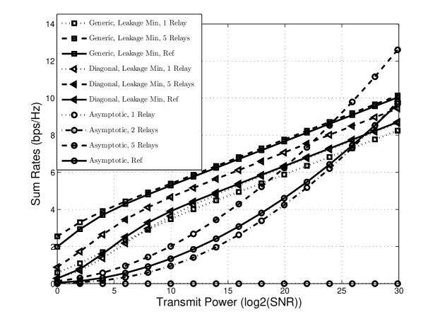
Figure 3: Coding on the edge with leakage minimization and asymptotic design, with different number of relays

However, if we deal with the relay constructed diagonal channels by using the analytical asymptotic design (Cadambe-Jafar scheme) for frequency selective channels [1], each user could approach $1/2$ DoF regardless of the number of $K$ users in the network. Take the 3-user network as an example to apply Cadambe-Jafar scheme in this relay network. The system equation (2) needs to be modified a little: let ${\mathrm{{V}}_{1}}\in\mathbb{C}^{T\times(n+1)}$, ${\mathrm{{V}}_{2}}\in\mathbb{C}^{T\times n}$, ${\mathrm{{V}}_{3}}\in\mathbb{C}^{T\times n}$, $T=2n+1\text{ }$, where $n$ is a positive integer. Thus DoF for the three users are not symmetric here and set as $\frac{n+1}{2n+1}$, $\frac{n}{2n+1}$, $\frac{n}{2n+1}$ respectively. When $n$ is large enough, each user could approach $1/2$ DoF. Design the aligned interference subspace at each user as following:

$$\mathrm{\Theta}_{12}\mathrm{V}_{2}=\mathrm{\Theta}_{13}\mathrm{{V}}_{3},\mathrm{\Theta}_{23}\mathrm{V}_{3}\prec\mathrm{\Theta}_{21}\mathrm{{V}}_{1},\mathrm{\Theta}_{32}\mathrm{V}_{2}\prec\mathrm{\Theta}_{31}\mathrm{{V}}_{1}$$ (9)

Then [1] proposed the following analytical design for each precoding matrix to satisfy (9):

$$\mathrm{{A}} =\mathrm{\Theta}_{12}\mathrm{\Theta}_{21}^{-1}\mathrm{\Theta}_{23}\mathrm{\Theta}_{32}^{-1}\mathrm{\Theta}_{31}\mathrm{\Theta}_{13}^{-1}$$ (10)

$$\mathrm{{V}}_{1} =[\mathrm{w}\ \mathrm{w}\mathrm{A}\ \mathrm{w}\mathrm{A}^{2}\ \cdots\ \mathrm{w}\mathrm{A}^{n}]$$

$$\mathrm{{V}}_{3} =\mathrm{\Theta}_{21}\mathrm{\Theta}_{23}^{-1}[\mathrm{w}\mathrm{A}\ \mathrm{w}\mathrm{A}^{2}\ \cdots\ \mathrm{w}\mathrm{A}^{n}]$$

$$\mathrm{{V}}_{2} =\mathrm{\Theta}_{31}\mathrm{\Theta}_{32}^{-1}[\mathrm{w}\ \mathrm{w}\mathrm{A}\ \cdots\ \mathrm{w}\mathrm{A}^{n-1}]$$

where $\mathrm{w}=[1\ 1\ \cdots\ 1]^{{\dagger}}\in\mathbb{C}^{(2n+1)\times 1}$. In this way, the three-user network could approach $3/2$ DoF eventually. It is important to highlight that this scheme could be extended to arbitrary $K$-user case. Then (9) and (10) are upgraded to a more complicated form accordingly [1]. The achievable multiplexing gain of the network becomes $\frac{(n+1)^{N}+(K-1)n^{N}}{(n+1)^{N}+n^{N}}$, where $N=(K-1)(K-2)-1$, $n$ is non-negative integer. As a result each user could approach $1/2$ DoF.

Numerical results are shown in Fig. 3. In the 3-user network, let $n=10$ so that the time extension length $T=21$. There are four cases: relay number $L=1$, $L=2$, $L=5$, and no relay. In addition, a case of frequency selective channel with 21 dimensions for all nodes is introduced as a reference. The four cases using the asymptotic design are denoted by ‘Asymptotic’. When the channels are generated by 2 relays or 5 relays, each user could obtain the same DoF as the reference frequency selective channel case. However, when the channels are generated by only 1 relay, each user obtains zero rate, and zero DoF, i.e. the interference alignment scheme fails.

The reason for the failure of the case of $L=1$ is investigated as following. For $L=1$ relay, (3) becomes:

$$\Theta_{ji}=f_{j1}\mathrm{G}_{1}h_{1i}$$ (11)

Notice $\mathrm{G}_{l}$ is diagonal as in (7), then the asymptotic design in (10) degenerates to the following form:

$$\alpha =f_{11}h_{12}(f_{21}h_{11})^{-1}f_{21}h_{13}(f_{31}h_{12})^{-1}f_{31}h_{11}(f_{11}h_{13})^{-1}$$ (12)

$$\mathrm{{A}} =\alpha\mathrm{I}_{T}$$

$$\mathrm{{V}}_{1} =[\mathrm{w}\ \alpha\mathrm{w}\ \alpha^{2}\mathrm{w}\ \cdots\ \alpha^{n}\mathrm{w}]$$

$$\mathrm{{V}}_{3} =f_{21}h_{11}(f_{21}h_{13})^{-1}[\alpha\mathrm{w}\ \alpha^{2}\mathrm{w}\ \cdots\ \alpha^{n}\mathrm{w}]$$

$$\mathrm{{V}}_{2} =f_{31}h_{11}(f_{31}h_{12})^{-1}[\mathrm{w}\ \alpha\mathrm{w}\ \cdots\ \alpha^{n-1}\mathrm{w}]$$

where $\alpha$ is scalar coefficient equal to 1, and $\mathrm{I}_{T}$ is an identity matrix. Observe in (12) the three precoding matrices $\mathrm{{V}}_{1}$, $\mathrm{{V}}_{2}$, $\mathrm{{V}}_{3}$ have only rank 1 because all $\Theta_{ji}$ are linear dependent to be eliminated, so that the asymptotic solution fails due to the lack of channel randomness or relativity in [1], which is the core idea of the IA mechanism. Similarly, in the $K$-user case, the asymptotic solution also fails when there is only 1 relay. Meanwhile recall the numerical result by leakage minimization algorithm in equivalent MIMO scheme, the achieved DoF is low but non-zero.

Comparing with the case of $L=2$, the relay generated diagonal channel in (8) becomes:

$$\Theta_{ji}=f_{j1}\mathrm{G}_{1}h_{1i}+f_{j2}\mathrm{G}_{2}h_{2i}$$ (13)

It needs to be proved that $\Theta_{ji}$ are not linear dependent to lose channel randomness with the following lemma.

Lemma 1

$\Theta_{ji}$ and $\Theta_{nm}$ are linear independent almost surely for arbitrary non-identical $(j,i)$ and $(n,m)$.

Proof: Assume

$\exists\beta_{1},\beta_{2}\in\mathbb{C}$. $\beta_{1},\beta_{2}\neq 0$, such that $\beta_{1}\Theta_{ji}+\beta_{2}\Theta_{nm}=\mathrm{0}$.

Expand and group by $\mathrm{G}_{1}$ and $\mathrm{G}_{2}$ to:

$(\beta_{1}f_{j1}h_{1i}+\beta_{2}f_{n1}h_{1m})\mathrm{G}_{1}+(\beta_{1}f_{j2}h_{2i}+\beta_{2}f_{n2}h_{2m})\mathrm{G}_{2}=\mathrm{0}$ .

$\mathrm{G}_{1}$ and $\mathrm{G}_{2}$ are arbitrary generic diagonal matrices, therefore almost surely the coefficients are zeros, i.e.

$(\beta_{1}f_{j1}h_{1i}+\beta_{2}f_{n1}h_{1m})=0,(\beta_{1}f_{j2}h_{2i}+\beta_{2}f_{n2}h_{2m})=0$.

Forming the ratio $-\frac{\beta_{1}}{\beta_{1}}$, so we have $\frac{f_{j1}h_{1i}}{f_{n1}h_{1m}}=\frac{f_{j2}h_{2i}}{f_{n2}h_{2m}}$.

Since $f_{j1},h_{1i},f_{n1},h_{1m},f_{j2},h_{2i},f_{n2},h_{2m}$ are all random independent scalars, the equality fails almost surely. So that $\beta_{1}$, $\beta_{2}$ do not exist almost surely. Then $\Theta_{ji}$ and $\Theta_{nm}$ are linearly independent almost surely.  $\square$

Notice ‘almost surely’ cases are recognized as successful interference alignment [1]. Lemma 1 shows that $\Theta_{12}\Theta_{21}^{-1}$,$\Theta_{23}\Theta_{32}^{-1}$, and $\Theta_{31}\Theta_{13}^{-1}$ are not scaled identity matrices, therefore their total product, $\mathrm{A}$, is not a scaled identity matrix almost surely considering channel relativity of these three terms. As a result the asymptotic design in (10) still works here, rather than degenerating to the form (12). In summary, Lemma 1 reveals that two or more relays can generate channel randomness or channel relativity in the equivalent channels with problems in (11) and (12) successfully prevented. Then the asymptotic design in (10) can be applied successfully.

IV Role of Relay in Precoding Scheme in Constant Channels

The above 3-user case reveals a critical issue for the constant channel to implement interference alignment. Therefore it is important to look into general $K$-user networks, as well as different class of IA schemes. In this section, for the general scenarios of relay networks, the model is shown in Fig. 2 : define nodes ${I}_{1},{I}_{2},\cdots,{I}_{K}$ as sources and ${J}_{1},\cdots,{J}_{K-1},{J}_{K}$ as destinations, whereas each $I_{k}$ communicates with each ${J}_{k}$ via relays ${R}_{1},{R}_{2},\cdots,{R}_{L}$. Relays are half-duplex so that the transmission procedure consists of two stages where relays forward data in the second stage. Interference alignment is designed with the following strategy: relays construct equivalent channels; source and destination nodes proceed precoding and zero-forcing, i.e. coding at the edge as [20] claimed. The objective is still to approach 1/2 due DoF (exclude duplex factor) for every user, which is quite difficult and non-trivial for a relay network under quasi-static channel condition. The work is published in [26] and submitted in [27].

IV-A Time-extended Signal Vector Alignment

The most common approach to implement IA in this network is the time-extended MIMO scheme as in [3], where $T$ consecutive symbols form one signal vector and IA is designed in the vector space. The above example of 3-user network as in equations (7) and (8) exactly constructs the relay gain matrix $\mathrm{G}_{l}$ and equivalent channels $\Theta_{ji}$ with this time-extended MIMO approach. Therefore, it is important to extend the design to arbitrary $K$-user networks, and look into the same issue caused by constant channels with single relay in the network.

$\mathrm{G}_{l}$ and $\Theta_{ji}$ could be diagonal or generic. If they are generic, it is equivalent to MIMO channel constrained by feasibility conditions [25], so that each user could only approach $2/(K+1)$ DoF. If they are diagonal, the channel is equivalent to a frequency selective channel in [1, 28], then the asymptotic design of Cadambe-Jafar scheme could be applied. Notice [28] has the same core design structure as [1], so that the design of [28] is illustrated here for a general $K$-pair relay network as in the following form:

$$\mathrm{{\Phi}}_{ji} =\mathrm{\Theta}_{j1}^{-1}\mathrm{\Theta}_{ji}\mathrm{\Theta}_{1i}^{-1}\mathrm{\Theta}_{13}\hskip 8.53581pt\forall j,i\in\mathcal{K}\setminus\{1\}$$ (14)

$$\mathrm{{V}}_{3} =\left\{\mathrm{{\Phi}}_{23}^{-1}\prod_{(j,i)\in\mathcal{A}}\left(\mathrm{{\Phi}}_{23}^{-1}\mathrm{{\Phi}}_{ji}\right)^{n_{ji}}\cdot\mathbf{1}_{T}\ \Big{|}\sum_{(j,i)\in\mathcal{A}}n_{ji}\leq n^{*}\right\}$$ (15)

$$\mathrm{{V}}_{1} =\left\{\prod_{(j,i)\in\mathcal{A}}\left(\mathrm{{\Phi}}_{23}^{-1}\mathrm{{\Phi}}_{ji}\right)^{n_{ji}}\cdot\mathbf{1}_{T}\ \Big{|}\sum_{(j,i)\in\mathcal{A}}n_{ji}\leq n^{*}+1\right\}$$

$$\mathrm{{V}}_{i} =\mathrm{\Theta}_{1i}^{-1}\mathrm{\Theta}_{13}\mathrm{V_{3}}\hskip 8.53581pt\forall i\in\mathcal{K}\setminus\{1,3\}$$

where $\mathrm{V}_{i}\in\mathbb{C}^{T\times d_{i}}$ is the precoding matrix for arbitrary source $I_{i},i\neq 1,3$, which contains $d_{i}$ input streams. $\mathcal{A}=\left\{(j,i)\ |\ j,i\in\mathcal{K}\setminus\{1\},j\neq i,(j,i)\neq(2,3)\right\}$. $\mathbf{1}_{T}\in\mathbb{C}^{T\times 1}$ is the all one vector, $n^{*}$ is integer. Notice $T=\binom{n^{*}+N+1}{N}+\binom{n^{*}+N}{N}$ and $N=(K-1)(K-2)-1$. $\mathrm{{V}}_{1}$ has a dimension of $T\times\binom{n^{*}+N+1}{N}$; $\mathrm{{V}}_{i}$ has a dimension of $T\times\binom{n^{*}+N}{N}$, $\forall i\neq 1$. So that each user could approach $1/2$ DoF when $n^{*}$ is large for arbitrary $K$.

IV-A1 The case when the network has single relay, $L=1$

However, in the special case when $L=1$, this scheme does not work. The reason is easily shown in the equations (3) and (14) as following:

$$\mathrm{{\Phi}}_{ji}\cdot\mathbf{1}_{T}=(\mathrm{h}_{J_{j}R_{1}}\mathrm{G}_{1}\mathrm{h}_{R_{1}I_{1}})^{-1}(\mathrm{h}_{J_{j}R_{1}}\mathrm{G}_{1}\mathrm{h}_{R_{1}I_{i}})$$ (16)

$$\hskip 39.83385pt\cdot(\mathrm{h}_{J_{1}R_{1}}\mathrm{G}_{1}\mathrm{h}_{R_{1}I_{1}})^{-1}(\mathrm{h}_{J_{1}R_{1}}\mathrm{G}_{1}\mathrm{h}_{R_{1}I_{3}})\cdot\mathbf{1}_{T}$$

$$\hskip 14.22636pt=\mathrm{h}_{J_{j}R_{1}}^{-1}\mathrm{h}_{R_{1}I_{1}}^{-1}\mathrm{h}_{J_{j}R_{1}}\mathrm{h}_{R_{1}I_{i}}\mathrm{h}_{J_{1}R_{1}}^{-1}\mathrm{h}_{R_{1}I_{1}}^{-1}\mathrm{h}_{J_{1}R_{1}}\mathrm{h}_{R_{1}I_{3}}\cdot\mathbf{1}_{T}$$

Apply (LABEL:Phi-1R) to the precoding solutions of (15), then we could observe column subspace of $\mathrm{{V}}_{i},\forall i\in\mathcal{K}$ in (15) collapses to one dimensional space parallel to $\mathbf{1}_{T}$. It means the signal subspace of $\mathrm{{V}}_{i}$ degenerates so that all the transmissions fail to obtain DoF. The following remark is summarized.

Remark 1

For the equivalent channels generated by single relay, interference alignment is not feasible to approach 1/2 DoF for every user by using existing asymptotic designs of [28, 1].

IV-A2 The case when the network has at least two relays, $L\geq 2$

While for the case of $L\geq 2$, asymptotic IA scheme could be much likely applied to obtain $K/2$ DoF of this network for arbitrary $K$. As a primitive investigation, set $L=2$. The key is to prove that the column subspace of $\mathrm{{V}}_{i},\forall i\in\mathcal{K}$ in (15) almost surely maintains its rank. First, we need to look at the core elements $\mathrm{{\Phi}}_{23}^{-1}\mathrm{{\Phi}}_{ji}$ which constitute $\mathrm{{V}}_{i}$. The objective is to prove all the $\mathrm{{\Phi}}_{23}^{-1}\mathrm{{\Phi}}_{ji}$ terms are linear independent. Then the expanded form is as in equation (LABEL:Phi-2R) and proved through the following three lemmas:

$$\mathrm{{\Phi}}_{23}^{-1}\mathrm{{\Phi}}_{ji}=\frac{(\mathrm{h}_{J_{2}R_{1}}\mathrm{G}_{1}\mathrm{h}_{R_{1}I_{1}}+\mathrm{h}_{J_{2}R_{2}}\mathrm{G}_{2}\mathrm{h}_{R_{2}I_{1}})}{(\mathrm{h}_{J_{j}R_{1}}\mathrm{G}_{1}\mathrm{h}_{R_{1}I_{1}}+\mathrm{h}_{J_{j}R_{2}}\mathrm{G}_{2}\mathrm{h}_{R_{2}I_{1}})}\bullet$$ (17)

$$\frac{(\mathrm{h}_{J_{j}R_{1}}\mathrm{G}_{1}\mathrm{h}_{R_{1}I_{i}}+\mathrm{h}_{J_{j}R_{2}}\mathrm{G}_{2}\mathrm{h}_{R_{2}I_{i}})(\mathrm{h}_{J_{1}R_{1}}\mathrm{G}_{1}\mathrm{h}_{R_{1}I_{3}}+\mathrm{h}_{J_{1}R_{2}}\mathrm{G}_{2}\mathrm{h}_{R_{2}I_{3}})}{(\mathrm{h}_{J_{2}R_{1}}\mathrm{G}_{1}\mathrm{h}_{R_{1}I_{3}}+\mathrm{h}_{J_{2}R_{2}}\mathrm{G}_{2}\mathrm{h}_{R_{2}I_{3}})(\mathrm{h}_{J_{1}R_{1}}\mathrm{G}_{1}\mathrm{h}_{R_{1}I_{i}}+\mathrm{h}_{J_{1}R_{2}}\mathrm{G}_{2}\mathrm{h}_{R_{2}I_{i}})}$$

Lemma 2

$\mathrm{G}_{1}^{3}\mathbf{1}_{T}$, $\mathrm{G}_{1}^{2}\mathrm{G}_{2}\mathbf{1}_{T}$, $\mathrm{G}_{1}\mathrm{G}_{2}^{2}\mathbf{1}_{T}$, $\mathrm{G}_{2}^{3}\mathbf{1}_{T}$ are linear independent almost surely.

Proof: Let $\mathrm{G}_{1}^{-1}\mathrm{G}_{2}=\mathrm{Diag}\{\lambda_{1},\cdots,\lambda_{T}\}$. $\mathrm{Diag}\{\cdot\}$ denotes the function to generate a diagonal matrix with all elements in the set. Suppose the lemma is false, then $(\mathrm{G}_{1}^{-1}\mathrm{G}_{2})^{3}\mathbf{1}_{T}$, $(\mathrm{G}_{1}^{-1}\mathrm{G}_{2})^{2}\mathbf{1}_{T}$, $\mathrm{G}_{1}^{-1}\mathrm{G}_{2}\mathbf{1}_{T}$, $\mathbf{1}_{T}$ are linear dependent. So that there exist non-zero $\alpha_{1},\alpha_{2},\alpha_{3},\alpha_{4}$ satisfying the element-wise equations of $\alpha_{1}\lambda_{t}^{3}+\alpha_{2}\lambda_{t}^{2}+\alpha_{3}\lambda_{t}+\alpha_{4}=0$, $\forall t=1,\ldots,T$. Since $\mathrm{G}_{1},\mathrm{G}_{2},\lambda_{1},\cdots,\lambda_{T}$ are random generated independent parameters, and rank-3 polynomials could not have $T$ non-identical roots almost surely, so it proves the lemma is true almost surely.  $\square$

Lemma 3

$\mathrm{{\Phi}}_{23}^{-1}\mathrm{{\Phi}}_{ji}\mathbf{1}_{T}$ and $\mathrm{{\Phi}}_{23}^{-1}\mathrm{{\Phi}}_{nm}\mathbf{1}_{T}$ are linear independent almost surely for arbitrary non-identical $(j,i),(n,m)\in\mathcal{A}$, where $\mathcal{A}=\left\{(j,i)\ |\ j,i\in\mathcal{K}\setminus\{1\},j\neq i,(j,i)\neq(2,3)\right\}$.

Proof:

Suppose $\exists\text{ non-zero }\beta_{a},\beta_{b}$ satisfying $\beta_{a}\mathrm{{\Phi}}_{23}^{-1}\mathrm{{\Phi}}_{ji}\mathbf{1}_{T}+\beta_{b}\mathrm{{\Phi}}_{23}^{-1}\mathrm{{\Phi}}_{nm}\mathbf{1}_{T}=\mathbf{0}_{T}$, where $\mathbf{0}_{T}\in\mathbb{C}^{T\times 1}$ denotes an all-zero vector. Derived from (14), the following equation is obtained:

$$\beta_{a}\mathrm{\Theta}_{ji}\mathrm{\Theta}_{n1}\mathrm{\Theta}_{1m}\mathbf{1}_{T}+\beta_{b}\mathrm{\Theta}_{nm}\mathrm{\Theta}_{j1}\mathrm{\Theta}_{1i}\mathbf{1}_{T}=\mathbf{0}_{T}$$ (18)

By using (3) with (18), further we have equation (LABEL:expand-2).

$$(\beta_{a}\mathrm{h}_{J_{j}R_{1}}\mathrm{h}_{R_{1}I_{i}}\mathrm{h}_{J_{n}R_{1}}\mathrm{h}_{R_{1}I_{1}}\mathrm{h}_{J_{1}R_{1}}\mathrm{h}_{R_{1}I_{m}}+\beta_{b}\mathrm{h}_{J_{n}R_{1}}\mathrm{h}_{R_{1}I_{m}}\mathrm{h}_{J_{j}R_{1}}\mathrm{h}_{R_{1}I_{1}}\mathrm{h}_{J_{1}R_{1}}\mathrm{h}_{R_{1}I_{i}})\cdot\mathrm{G}_{1}^{3}\mathbf{1}_{T}$$ (19)

$$+[\beta_{a}(\mathrm{h}_{J_{j}R_{1}}\mathrm{h}_{R_{1}I_{i}}\mathrm{h}_{J_{n}R_{1}}\mathrm{h}_{R_{1}I_{1}}\mathrm{h}_{J_{1}R_{2}}\mathrm{h}_{R_{2}I_{m}}+\mathrm{h}_{J_{j}R_{1}}\mathrm{h}_{R_{1}I_{i}}\mathrm{h}_{J_{n}R_{2}}\mathrm{h}_{R_{2}I_{1}}\mathrm{h}_{J_{1}R_{1}}\mathrm{h}_{R_{1}I_{m}}+$$

$$\hskip 25.60747pt\mathrm{h}_{J_{j}R_{2}}\mathrm{h}_{R_{2}I_{i}}\mathrm{h}_{J_{n}R_{1}}\mathrm{h}_{R_{1}I_{1}}\mathrm{h}_{J_{1}R_{1}}\mathrm{h}_{R_{1}I_{m}})+\beta_{b}(\mathrm{h}_{J_{n}R_{1}}\mathrm{h}_{R_{1}I_{m}}\mathrm{h}_{J_{j}R_{1}}\mathrm{h}_{R_{1}I_{1}}\mathrm{h}_{J_{1}R_{2}}\mathrm{h}_{R_{2}I_{i}}$$

$$\hskip 14.22636pt+\mathrm{h}_{J_{n}R_{1}}\mathrm{h}_{R_{1}I_{m}}\mathrm{h}_{J_{j}R_{2}}\mathrm{h}_{R_{2}I_{1}}\mathrm{h}_{J_{1}R_{1}}\mathrm{h}_{R_{1}I_{i}}+\mathrm{h}_{J_{n}R_{2}}\mathrm{h}_{R_{2}I_{m}}\mathrm{h}_{J_{j}R_{1}}\mathrm{h}_{R_{1}I_{1}}\mathrm{h}_{J_{1}R_{1}}\mathrm{h}_{R_{1}I_{i}})]\cdot\mathrm{G}_{1}^{2}\mathrm{G}_{2}\mathbf{1}_{T}$$

$$+[\beta_{a}(\mathrm{h}_{J_{j}R_{1}}\mathrm{h}_{R_{1}I_{i}}\mathrm{h}_{J_{n}R_{2}}\mathrm{h}_{R_{2}I_{1}}\mathrm{h}_{J_{1}R_{2}}\mathrm{h}_{R_{2}I_{m}}+\mathrm{h}_{J_{j}R_{2}}\mathrm{h}_{R_{2}I_{i}}\mathrm{h}_{J_{n}R_{1}}\mathrm{h}_{R_{1}I_{1}}\mathrm{h}_{J_{1}R_{2}}\mathrm{h}_{R_{2}I_{m}}+$$

$$\hskip 25.60747pt\mathrm{h}_{J_{j}R_{2}}\mathrm{h}_{R_{2}I_{i}}\mathrm{h}_{J_{n}R_{2}}\mathrm{h}_{R_{2}I_{1}}\mathrm{h}_{J_{1}R_{1}}\mathrm{h}_{R_{1}I_{m}})+\beta_{b}(\mathrm{h}_{J_{n}R_{1}}\mathrm{h}_{R_{1}I_{m}}\mathrm{h}_{J_{j}R_{2}}\mathrm{h}_{R_{2}I_{1}}\mathrm{h}_{J_{1}R_{2}}\mathrm{h}_{R_{2}I_{i}}$$

$$\hskip 14.22636pt+\mathrm{h}_{J_{n}R_{2}}\mathrm{h}_{R_{2}I_{m}}\mathrm{h}_{J_{j}R_{1}}\mathrm{h}_{R_{1}I_{1}}\mathrm{h}_{J_{1}R_{2}}\mathrm{h}_{R_{2}I_{i}}+\mathrm{h}_{J_{n}R_{2}}\mathrm{h}_{R_{2}I_{m}}\mathrm{h}_{J_{j}R_{2}}\mathrm{h}_{R_{2}I_{1}}\mathrm{h}_{J_{1}R_{1}}\mathrm{h}_{R_{1}I_{i}})]\cdot\mathrm{G}_{1}\mathrm{G}_{2}^{2}\mathbf{1}_{T}$$

$$+(\beta_{a}\mathrm{h}_{J_{j}R_{2}}\mathrm{h}_{R_{2}I_{i}}\mathrm{h}_{J_{n}R_{2}}\mathrm{h}_{R_{2}I_{1}}\mathrm{h}_{J_{1}R_{2}}\mathrm{h}_{R_{2}I_{m}}+\beta_{b}\mathrm{h}_{J_{n}R_{2}}\mathrm{h}_{R_{2}I_{m}}\mathrm{h}_{J_{j}R_{2}}\mathrm{h}_{R_{2}I_{1}}\mathrm{h}_{J_{1}R_{2}}\mathrm{h}_{R_{2}I_{i}})\cdot\mathrm{G}_{2}^{3}\mathbf{1}_{T}$$

$$=\mathbf{0}_{T}$$

In (LABEL:expand-2), since $\mathrm{G}_{1}^{3}\mathbf{1}_{T}$, $\mathrm{G}_{1}^{2}\mathrm{G}_{2}\mathbf{1}_{T}$, $\mathrm{G}_{1}\mathrm{G}_{2}^{2}\mathbf{1}_{T}$, $\mathrm{G}_{2}^{3}\mathbf{1}_{T}$ are actually four independent $T$-dimensional bases, then all their coefficients must be zero. We obtain another four linear equations about $\beta_{a}$, $\beta_{b}$, with coefficients composed of $\mathrm{h}_{J_{j}R_{1}},\mathrm{h}_{R_{1}I_{i}},\mathrm{h}_{J_{j}R_{2}},\mathrm{h}_{R_{2}I_{i}}$, which are all random independent scalar values of the channels. Therefore the solutions of $\beta_{a},\beta_{b}$ are zero almost surely, which contradicts the initial non-zero assumption. So that it proves the lemma.

$\square$

Lemma 4

All vectors in $\{\mathrm{{\Phi}}_{23}^{-1}\mathrm{{\Phi}}_{ji}\mathbf{1}_{T},(j,i)\in\mathcal{A}\}$ are linear independent almost surely, where $\mathcal{A}=\left\{(j,i)\ |\ j,i\in\mathcal{K}\setminus\{1\},j\neq i,(j,i)\neq(2,3)\right\}$.

Proof:

The procedure is similar to Lemma 3. Only notice that the set contains $N$ vectors. The new equation corresponding to (18) has degree of $2N-1$ over $\Theta_{ji}$. Expand to a new equation corresponding to (LABEL:expand-2), similarly there are totally $2N$ $T$-dimensional bases such as $\mathrm{G}_{1}^{2N}\mathbf{1}_{T},\mathrm{G}_{1}^{2N-1}\mathrm{G}_{2}^{1}\mathbf{1}_{T}$ etc. Then there are $2N$ linear equations about $N$ variables $\beta_{1},\ldots,\beta_{N}$, which are forced to be zero. So that the independency is proved.  $\square$

Finally, in addition, consider the linear independency of the exponentiation terms of $\mathrm{{\Phi}}_{23}^{-1}\mathrm{{\Phi}}_{ji}\mathbf{1}_{T}$ in the precoders $\mathrm{V}_{i},\forall i\in\mathcal{K}$ in (15). Because the signal dimension $T$ is large enough to afford the number of bases in space, so that all $\mathrm{V}_{i},\forall i\in\mathcal{K}$ are possibly well-conditioned to implement interference alignment. However, it needs further rigorous proof in our future work.

In summary, the comparison of the cases $L=1$ and $L\geq 2$ in signal vector space illustrates that in single antenna constant relay channels, single relay is not able to provide channel randomness or relativity which is the key to interference alignment, while at least two relays are necessary to provide this feature to approach 1/2 DoF (excluding duplex factor) for every user.

IV-B Number-Based Signal Level Alignment

Besides signal vector alignment for single antenna constant channels, there is another major class of schemes called signal level interference alignment. There are several approaches to investigate signal level alignment, including lattice coding, deterministic models, and number theory. Among these approaches, IA on the number domain is a very novel and canonical method. While our focus in the following work is to show, in relay connected constant channels, in a similar manner to vector alignment scheme, how level alignment would also face the applicability issue of existing designs when there is only one relay and the issue solved when there are at least two relays.

IV-B1 Basic Concept and Design Procedure

At first, signal level could be viewed on the rational number scale which represents infinite fractional DoF [29]. Then Khintchine-Groshev theorem also reveals that the field of real numbers is rich enough to be equivalent to vector space to design IA. Furthermore, [30, Theorem 7] uses a generalized version of Khintchin-Groshev theorem to extend the designs to complex channels. In real channels, DoF is defined as $d_{\mathrm{Real}}=\lim_{P\rightarrow\infty}\frac{C_{\mathrm{sum}}}{1/2\log_{2}(P)}$ while in complex channel DoF is defined as $d_{\mathrm{Complex}}=\lim_{P\rightarrow\infty}\frac{C_{\mathrm{sum}}}{\log_{2}(P)}$ where $C_{\mathrm{sum}}$ is sum capacity and $P$ is transmission power.

By using this Motahari-Khandani scheme in [29, 30], $K$-user single antenna constant channels could approach $K/2$ DoF. Since the objective in this work is to study the role of relays, the core structure and procedure of IA are briefly described in a complex channel setting.

Define $\mathbf{u}_{k}=[u_{k}^{(1)}u_{k}^{(2)}\cdots u_{k}^{(d_{k})}]$ as the number of $d_{k}$ datastreams sent from node $I_{k}$ to node $J_{k}$, $k\in\mathcal{K}$. $u_{k}^{(m)}\in(-Q,Q)_{\mathbb{Z}},1\leq m\leq d_{k}$, i.e. belongs to an integer constellation. Each datastream is multiplied by a number $\nu_{k}^{(m)}\in\mathbb{C}$, which is called a modulation pseudo-vector serving as distinct directions. In order to satisfy the power constraint and control the minimum distance of the received constellation, transmission signals should be scaled with a constant $\lambda$.

In the meanwhile, each relay node $R_{l}$ generates a random gain to be a rational number $g_{l}\in\mathbb{Q}$ and the equivalent channel from $I_{i}$ to $J_{k}$ is as following:

$$\theta_{ki}=\sum_{l=1}^{L}\mathrm{h}_{J_{k}R_{l}}\cdot{g}_{l}\cdot\mathrm{h}_{R_{l}I_{i}}$$ (20)

Then the received signal at destination node $J_{k}$ is:

$$y_{k}=\lambda\theta_{kk}\sum_{m=1}^{d_{k}}\nu_{k}^{(m)}u_{k}^{(m)}+\sum_{i=1,i\neq k}^{K}\lambda\theta_{ki}\sum_{m=1}^{d_{i}}\nu_{i}^{(m)}u_{i}^{(m)}$$ (21)

According to [29, 30], the structure design of pseudo-vectors $\nu_{k}^{(m)}$ on number domain is similar to the design of $\mathrm{V}_{i}$ in vector space of [28], however there exists notable difference as well. In this design, all $\nu_{k}^{(m)},1\leq m\leq d_{k}$ belong to a set $\mathcal{B}_{\nu_{k}}$:

$$\mathcal{B}_{\nu_{k}} =\left\{\prod_{j=1}^{K}\prod_{i=1,j\neq i}^{K}\theta_{ji}^{\alpha_{ji}}\Big{|}\begin{aligned} &0\leq\alpha_{ji}\leq n-1\ \ \ i=k,j\neq k\\ &0\leq\alpha_{ji}\leq n\ \ \ \ \ \ \ \ \text{Otherwise}\end{aligned}\right\}$$ (22)

$n$ is integer, so that the number of streams $d_{k}=|\mathcal{B}_{\nu_{k}}|=n^{K-1}(n+1)^{(K-1)^{2}}$.

For destination node $J_{k}$, the received signal space of (21) contains desired signal subspace formed by $\theta_{kk}\mathcal{B}_{\nu_{k}}$ and interference subspace formed by $\theta_{ki}\mathcal{B}_{\nu_{i}},i\neq k$. Observe all the interference subspaces overlap to the same set of $\mathcal{B}_{\nu_{k}}^{\prime}$:

$$\mathcal{B}_{\nu_{k}}^{\prime} =\left\{\prod_{j=1}^{K}\prod_{i=1,j\neq i}^{K}\theta_{ji}^{\alpha_{ji}}\Big{|}0\leq\alpha_{ji}\leq n\right\}$$ (23)

So that $|\mathcal{B}_{\nu_{k}}^{\prime}|=(n+1)^{K(K-1)}$. Meanwhile the desired signal subspace $\theta_{kk}\mathcal{B}_{\nu_{k}}$ and interference subspace $\mathcal{B}_{\nu_{k}}^{\prime}$ are distinct. According to [29, Theorem 6], the total DoF is $\frac{Kn^{K-1}(n+1)^{(K-1)^{2}}}{n^{K-1}(n+1)^{(K-1)^{2}}+(n+1)^{K(K-1)}+1}$, which approaches $K/2$ when $n$ is large.

IV-B2 Issue in the Three-User Special Case

In the three-user case, there is a special form of design in [29, Definition 1] presented as following:

$$\hskip 22.76219pty_{1}=\vartheta_{1}\cdot x_{1}+x_{2}+x_{3}+z_{1}$$ (24)

$$\hskip 22.76219pty_{2}=\vartheta_{2}\cdot x_{2}+x_{1}+x_{3}+z_{2}$$

$$\hskip 22.76219pty_{3}=\vartheta_{3}\cdot x_{3}+x_{1}+\vartheta_{0}\cdot x_{2}+z_{3}$$

$$\vartheta_{0}=\frac{\theta_{13}\theta_{21}\theta_{32}}{\theta_{12}\theta_{23}\theta_{31}},\vartheta_{1}=\frac{\theta_{11}\theta_{12}\theta_{23}}{\theta_{12}\theta_{21}\theta_{13}},\vartheta_{2}=\frac{\theta_{22}\theta_{13}}{\theta_{12}\theta_{23}},\vartheta_{3}=\frac{\theta_{33}\theta_{12}\theta_{21}}{\theta_{12}\theta_{23}\theta_{31}}$$

So that user 1 has the transmit directions $\{1,\vartheta_{0},\vartheta_{0}^{2},\ldots,\vartheta_{0}^{n}\}$, user 2 has the directions of $\{1,\vartheta_{0},\ldots,\vartheta_{0}^{n-1}\}$, and user 3 has the directions of $\{1,\vartheta_{0},\ldots,\vartheta_{0}^{n-1}\}$.

$\bullet$ If the network has only one relay, $L=1$, according to (20) and (24):

$$\vartheta_{0}=\frac{\mathrm{h}_{J_{1}R_{1}}\mathrm{h}_{R_{1}I_{3}}\mathrm{h}_{J_{2}R_{1}}\mathrm{h}_{R_{1}I_{1}}\mathrm{h}_{J_{3}R_{1}}\mathrm{h}_{R_{1}I_{2}}\cdot{g}_{1}^{3}}{\mathrm{h}_{J_{1}R_{1}}\mathrm{h}_{R_{1}I_{2}}\mathrm{h}_{J_{2}R_{1}}\mathrm{h}_{R_{1}I_{3}}\mathrm{h}_{J_{3}R_{1}}\mathrm{h}_{R_{1}I_{1}}\cdot{g}_{1}^{3}}=1$$ (25)

Then the encoding set $\{1,\vartheta_{0},\vartheta_{0}^{2},\ldots,\vartheta_{0}^{n}\}$ used by all three users collapses. The scheme of [29, 30] is not applicable to this case to support normal transmission with interference alignment.

$\bullet$If the network has two relays, $L=2$, IA scheme is applicable as proved by the following lemma:

Lemma 5

$\vartheta_{0}\neq 1$ holds almost surely, for random independent parameters $\mathrm{h}_{J_{j}R_{1}}$, $\mathrm{h}_{J_{j}R_{2}}$, $\mathrm{h}_{R_{1}I_{i}}$, $\mathrm{h}_{R_{2}I_{i}}$, $g_{1}$, $g_{2}$, where $i,j\in\mathcal{K}$.

Proof:

Suppose $\vartheta_{0}=1$, from (20) and (24), we have ${\theta_{13}\theta_{21}\theta_{32}}-{\theta_{12}\theta_{23}\theta_{31}}=0$, and expand it to the equation (LABEL:number-base-3user-vartheta-double).

$$(\mathrm{h}_{J_{1}R_{1}}\mathrm{h}_{R_{1}I_{3}}\mathrm{h}_{J_{2}R_{1}}\mathrm{h}_{R_{1}I_{1}}\mathrm{h}_{J_{3}R_{1}}\mathrm{h}_{R_{1}I_{2}}-\mathrm{h}_{J_{1}R_{1}}\mathrm{h}_{R_{1}I_{2}}\mathrm{h}_{J_{2}R_{1}}\mathrm{h}_{R_{1}I_{3}}\mathrm{h}_{J_{3}R_{1}}\mathrm{h}_{R_{1}I_{1}})\cdot g_{1}^{3}$$ (26)

$$+[(\mathrm{h}_{J_{1}R_{1}}\mathrm{h}_{R_{1}I_{3}}\mathrm{h}_{J_{2}R_{1}}\mathrm{h}_{R_{1}I_{1}}\mathrm{h}_{J_{3}R_{2}}\mathrm{h}_{R_{2}I_{2}}+\mathrm{h}_{J_{1}R_{1}}\mathrm{h}_{R_{1}I_{3}}\mathrm{h}_{J_{2}R_{2}}\mathrm{h}_{R_{2}I_{1}}\mathrm{h}_{J_{3}R_{1}}\mathrm{h}_{R_{1}I_{2}}+$$

$$\hskip 25.60747pt\mathrm{h}_{J_{1}R_{2}}\mathrm{h}_{R_{2}I_{3}}\mathrm{h}_{J_{2}R_{1}}\mathrm{h}_{R_{1}I_{1}}\mathrm{h}_{J_{3}R_{1}}\mathrm{h}_{R_{1}I_{2}})-(\mathrm{h}_{J_{1}R_{1}}\mathrm{h}_{R_{1}I_{2}}\mathrm{h}_{J_{2}R_{1}}\mathrm{h}_{R_{1}I_{3}}\mathrm{h}_{J_{3}R_{2}}\mathrm{h}_{R_{2}I_{1}}$$

$$\hskip 14.22636pt+\mathrm{h}_{J_{1}R_{1}}\mathrm{h}_{R_{1}I_{2}}\mathrm{h}_{J_{2}R_{2}}\mathrm{h}_{R_{2}I_{3}}\mathrm{h}_{J_{3}R_{1}}\mathrm{h}_{R_{1}I_{1}}+\mathrm{h}_{J_{1}R_{2}}\mathrm{h}_{R_{2}I_{2}}\mathrm{h}_{J_{2}R_{1}}\mathrm{h}_{R_{1}I_{3}}\mathrm{h}_{J_{3}R_{1}}\mathrm{h}_{R_{1}I_{1}})]\cdot g_{1}^{2}g_{2}$$

$$+[(\mathrm{h}_{J_{1}R_{1}}\mathrm{h}_{R_{1}I_{3}}\mathrm{h}_{J_{2}R_{2}}\mathrm{h}_{R_{2}I_{1}}\mathrm{h}_{J_{3}R_{2}}\mathrm{h}_{R_{2}I_{2}}+\mathrm{h}_{J_{1}R_{2}}\mathrm{h}_{R_{2}I_{3}}\mathrm{h}_{J_{2}R_{1}}\mathrm{h}_{R_{1}I_{1}}\mathrm{h}_{J_{3}R_{2}}\mathrm{h}_{R_{2}I_{2}}+$$

$$\hskip 25.60747pt\mathrm{h}_{J_{1}R_{2}}\mathrm{h}_{R_{2}I_{3}}\mathrm{h}_{J_{2}R_{2}}\mathrm{h}_{R_{2}I_{1}}\mathrm{h}_{J_{3}R_{1}}\mathrm{h}_{R_{1}I_{2}})-(\mathrm{h}_{J_{1}R_{1}}\mathrm{h}_{R_{1}I_{2}}\mathrm{h}_{J_{2}R_{2}}\mathrm{h}_{R_{2}I_{3}}\mathrm{h}_{J_{3}R_{2}}\mathrm{h}_{R_{2}I_{1}}$$

$$\hskip 14.22636pt+\mathrm{h}_{J_{1}R_{2}}\mathrm{h}_{R_{2}I_{2}}\mathrm{h}_{J_{2}R_{1}}\mathrm{h}_{R_{1}I_{3}}\mathrm{h}_{J_{3}R_{2}}\mathrm{h}_{R_{2}I_{1}}+\mathrm{h}_{J_{1}R_{2}}\mathrm{h}_{R_{2}I_{2}}\mathrm{h}_{J_{2}R_{2}}\mathrm{h}_{R_{2}I_{3}}\mathrm{h}_{J_{3}R_{1}}\mathrm{h}_{R_{1}I_{1}})]\cdot g_{1}g_{2}^{2}$$

$$+(\mathrm{h}_{J_{1}R_{2}}\mathrm{h}_{R_{2}I_{3}}\mathrm{h}_{J_{2}R_{2}}\mathrm{h}_{R_{2}I_{1}}\mathrm{h}_{J_{3}R_{2}}\mathrm{h}_{R_{2}I_{2}}-\mathrm{h}_{J_{1}R_{2}}\mathrm{h}_{R_{2}I_{2}}\mathrm{h}_{J_{2}R_{2}}\mathrm{h}_{R_{2}I_{3}}\mathrm{h}_{J_{3}R_{2}}\mathrm{h}_{R_{2}I_{1}})\cdot g_{2}^{3}$$

$$=0$$

In equation (LABEL:number-base-3user-vartheta-double), since $\{g_{1}^{3},g_{1}^{2}g_{2},g_{1}g_{2}^{2},g_{2}^{3}\}$ are independent number bases with measure of one, the corresponding coefficients must be all zeros. Observe $g_{1}^{3}$ and $g_{2}^{3}$ in (LABEL:number-base-3user-vartheta-double), their coefficients are indeed 0; while observe $g_{1}^{2}g_{2}$ and $g_{1}g_{2}^{2}$, their coefficients are non-zero with measure one, because of random selected parameters of $\mathrm{h}_{J_{j}R_{1}}$, $\mathrm{h}_{J_{j}R_{2}}$, $\mathrm{h}_{R_{1}I_{i}}$, $\mathrm{h}_{R_{2}I_{i}}$. As a result, it proves that $\vartheta_{0}\neq 1$.

$\square$

In summary, the comparison of the cases $L=1$ and $L=2$ shows that single relay is not able to provide channel randomness or relativity in the signal level alignment on number domain, while two relays are capable of provide this feature to approach 1/2 due DoF for every user.

IV-B3 Issue in the $K$-User General Case

Extend the study of the three-user case to the general $K$-user case.

$\bullet$If the network has only one relay, $L=1$, according to (20) and (22), the set $\mathcal{B}_{\nu_{k}}$ is presented in an equal form of set $\mathcal{B}_{\nu_{k}}^{L1}$:

$$\mathcal{B}_{\nu_{k}}^{L1} =\left\{\prod_{j=1}^{K}\prod_{i=1,j\neq i}^{K}(\mathrm{h}_{J_{j}R_{1}}\cdot{g}_{1}\cdot\mathrm{h}_{R_{1}I_{i}})^{\alpha_{ji}}\Big{|}\begin{aligned} &0\leq\alpha_{ji}\leq n-1\ i=k,j\neq k\\ &0\leq\alpha_{ji}\leq n\ \ \ \ \ \ \text{Otherwise}\end{aligned}\right\}$$ (27)

Counting the cardinality $|\mathcal{B}_{\nu_{k}}^{L1}|$ is complicated so that it is natural to think of attain an upperbound by relaxing and expanding the set $\mathcal{B}_{\nu_{k}}^{L1}$ to a new set $\bar{\mathcal{B}}_{\nu_{k}}^{L1}$. $\mathcal{B}_{\nu_{k}}^{L1}\subset\bar{\mathcal{B}}_{\nu_{k}}^{L1}$:

$$\bar{\mathcal{B}}_{\nu_{k}}^{L1} =\left\{\big{(}\prod_{j\in\mathcal{K}}\mathrm{h}_{J_{j}R_{1}}^{\tau_{j}}\big{)}\cdot\big{(}{g}_{1}^{\gamma}\big{)}\cdot\big{(}\prod_{i\in\mathcal{K}}\mathrm{h}_{R_{1}I_{i}}^{\varsigma_{i}}\big{)}\Big{|}\begin{aligned} &0\leq\gamma\leq nK^{2},0\leq\tau_{j},\varsigma_{i}\leq nK\\ &\sum_{j\in\mathcal{K}}\tau_{j}=\gamma,{\sum_{i\in\mathcal{K}}\varsigma_{i}}=\gamma\end{aligned}\right\}$$ (28)

Notice that $\mathcal{B}_{\nu_{k}}^{L1}\subset\bar{\mathcal{B}}_{\nu_{k}}^{L1}$, so that $|\mathcal{B}_{\nu_{k}}^{L1}|<|\bar{\mathcal{B}}_{\nu_{k}}^{L1}|$. Further loose the set by:

$$\mathcal{C}_{\gamma}=\{(\tau_{1},\tau_{2},\ldots,\tau_{K})|0\leq\tau_{j}\leq nK,\forall j\in\mathcal{K},\sum_{j\in\mathcal{K}}\tau_{j}=\gamma\}$$ (29)

$$\mathcal{D}_{\gamma}=\{(\tau_{1},\tau_{2},\ldots,\varsigma_{K})|0\leq\varsigma_{i}\leq nK,\forall i\in\mathcal{K},\sum_{i\in\mathcal{K}}\varsigma_{i}=\gamma\}$$

$$|\bar{\mathcal{B}}_{\nu_{k}}^{L1}|\leq\sum_{\gamma=0}^{nK^{2}}{|\mathcal{C}_{\gamma}|\cdot|\mathcal{D}_{\gamma}|}<\sum_{\gamma=0}^{nK^{2}}(nK+1)^{K}\cdot(nK+1)^{K}$$

Compare with the original due cardinality of (22):

$$\frac{|\mathcal{B}_{\nu_{k}}^{L1}|}{n^{K-1}(n+1)^{(K-1)^{2}}}<\frac{(nK^{2}+1)(nK+1)^{2K}}{n^{K-1}(n+1)^{(K-1)^{2}}}\xrightarrow[]{n\rightarrow\infty,K\rightarrow\infty}0$$ (30)

It reveals that in equivalent channels generated by single relay, $L=1$, the encoding set $\mathcal{B}_{\nu_{k}}$ degenerates to negligible size for large $n$ and $K$, i.e. Motahari-Khandani scheme [29, 30] is not applicable in this case to support normal transmission with interference alignment.

$\bullet$If the network has at least two relays, $L\geq 2$, we have similar conclusions as lemma 5 such that the precoding set are greatly expanded with independent elements to support normal transmission with interference alignment. It also needs further comprehensive validation and rigorous proof with exact requisite conditions.

IV-C Asymmetric Complex Signaling Alignment

Asymmetric complex signaling alignment is categorized into a class of phase alignment. It is proposed by Jafar as an effective measure to solve the problem of obtaining high DoF in constant interference channels [31]. However, the work in this thesis investigates if it is applicable to the relay generated equivalent interference channel.

It has been conjectured by H$\o$st, Madsen and Nosratinia that complex Gaussian interference channels with single antenna nodes and constant channel coefficients have only one degree-of-freedom regardless of the number of users [32]. Intuitively, this conjecture indicates the optimality of orthogonal medium access such as TDMA where each user is assigned a fraction of DoF and the sum DoF is equal to one. Original interference alignment [1, 33] provided a powerful tool to achieve $K/2$ DoF for $K$-user interference channels, only under the condition of time-varying or frequency-selective channel coefficients. However, in single antenna constant channels, it was not known if H$\o$st-Madsen-Nosratinia conjecture is right until the appearance of asymmetric complex signaling method.

By using asymmetric complex signal inputs, Jafar shows that at least 1.2 DoF are achievable on the complex 3-user interference channel with constant channel coefficients [31], without any assumption of time-variations/frequency-selectivity used in prior work. In conventional wireless systems only circularly symmetric complex Gaussian random variables are typically used in order to maximize entropy, while in asymmetric complex signaling the inputs are chosen to be complex but not circularly symmetric. For example, in an specific case of phase alignment, each transmitter uses only real valued Gaussian inputs, and ensures that interference at each receiver aligns in the imaginary dimension when the desired signal is in the real dimension of the complex space. This idea could be extended to general values of channel coefficients thereafter.

Detailed introduction is omitted here scheme, while the basic model and conclusion is briefly presented. First, each received complex signal is expressed in real values as following (noise is ignored for simplicity):

$$\left[\begin{aligned} \mathrm{Re}\{\mathrm{Y}_{i}\}\\ \mathrm{Im}\{\mathrm{Y}_{i}\}\end{aligned}\right]=\sum_{j=1}^{K}|\mathrm{H}_{ij}|\underbrace{\left[\begin{aligned} &\cos(\phi_{ij})\ -&\sin(\phi_{ij})\\ &\sin(\phi_{ij})\ &\cos(\phi_{ij})\end{aligned}\right]}_{\text{Defined as }U(\phi_{ij})}\left[\begin{aligned} \mathrm{Re}\{\mathrm{X}_{j}\}\\ \mathrm{Im}\{\mathrm{X}_{j}\}\end{aligned}\right]$$ (31)

where the complex output $\mathrm{Y}_{i}$ and complex input $\mathrm{X}_{j}$ are split into scalar counterparts of real values, and the complex scalar channel $\mathrm{H}_{ij}$ is expressed by its amplitude $|\mathrm{H}_{ij}|$ and a transformation matrix $U(\phi)$, which is a rotation matrix defined with the following properties:

$$U(\phi)^{-1} =U(-\phi)$$ (32)

$$U(\phi)U(\theta) =U(\theta)U(\phi)$$

$$U(\phi)U(\theta) =U(\phi+\theta)$$

With the new formulation, it is proved that the 3 user complex Gaussian interference channel with constant coefficients achieves 1.2 degrees-of-freedom if all of the following conditions are satisfied [31, Theorem 2]:

$$\phi_{J_{1}I_{3}}+\phi_{J_{2}I_{1}}-\phi_{J_{2}I_{3}}-\phi_{J_{1}I_{1}}\ \neq 0\ \mod{(\pi)}$$ (33)

$$\phi_{J_{1}I_{2}}+\phi_{J_{3}I_{1}}-\phi_{J_{3}I_{2}}-\phi_{J_{1}I_{1}}\ \neq 0\ \mod{(\pi)}$$

$$\phi_{J_{2}I_{1}}+\phi_{J_{3}I_{2}}-\phi_{J_{3}I_{1}}-\phi_{J_{2}I_{2}}\ \neq 0\ \mod{(\pi)}$$

$$\phi_{J_{2}I_{3}}+\phi_{J_{1}I_{2}}-\phi_{J_{1}I_{3}}-\phi_{J_{2}I_{2}}\ \neq 0\ \mod{(\pi)}$$

$$\phi_{J_{3}I_{2}}+\phi_{J_{1}I_{3}}-\phi_{J_{1}I_{2}}-\phi_{J_{3}I_{3}}\ \neq 0\ \mod{(\pi)}$$

$$\phi_{J_{3}I_{1}}+\phi_{J_{2}I_{3}}-\phi_{J_{2}I_{1}}-\phi_{J_{3}I_{3}}\ \neq 0\ \mod{(\pi)}$$

where $I_{1}$, $I_{2}$, $I_{3}$ are transmitter nodes and $J_{1}$, $J_{2}$, $J_{3}$ are receiver nodes. Notice the coditions of (33) are naturally satisfied almost surely for general 3-user networks. However, consider the relay networks as in Fig. 2, if there is only one relay, then the equivalent channel phase from transmitter $I_{i}$ to receiver $J_{j}$ is equal to the sum of phases from transmitter $I_{i}$ to relay $R_{1}$ and from relay $R_{1}$ to receiver $J_{j}$:

$$\phi_{J_{j}I_{i}}=\phi_{R_{1}I_{i}}+\phi_{J_{j}R_{1}}\ \mod{(\pi)}$$ (34)

Therefore, check the conditions of (33) again with (34), and it is easy to find out the following new results which make the design no longer available:

$$\phi_{J_{1}I_{3}}+\phi_{J_{2}I_{1}}-\phi_{J_{2}I_{3}}-\phi_{J_{1}I_{1}}\ =0\ \mod{(\pi)}$$ (35)

$$\phi_{J_{1}I_{2}}+\phi_{J_{3}I_{1}}-\phi_{J_{3}I_{2}}-\phi_{J_{1}I_{1}}\ =0\ \mod{(\pi)}$$

$$\phi_{J_{2}I_{1}}+\phi_{J_{3}I_{2}}-\phi_{J_{3}I_{1}}-\phi_{J_{2}I_{2}}\ =0\ \mod{(\pi)}$$

$$\phi_{J_{2}I_{3}}+\phi_{J_{1}I_{2}}-\phi_{J_{1}I_{3}}-\phi_{J_{2}I_{2}}\ =0\ \mod{(\pi)}$$

$$\phi_{J_{3}I_{2}}+\phi_{J_{1}I_{3}}-\phi_{J_{1}I_{2}}-\phi_{J_{3}I_{3}}\ =0\ \mod{(\pi)}$$

$$\phi_{J_{3}I_{1}}+\phi_{J_{2}I_{3}}-\phi_{J_{2}I_{1}}-\phi_{J_{3}I_{3}}\ =0\ \mod{(\pi)}$$

Similar to the time-extended signal vector scheme and the number-based signal level scheme, the remark for complex phase alignment is concluded:

Remark 2

For single antenna constant channels, if the $K$-pair users are connected by only one relay, then asymmetric complex signaling scheme would not work to obtain more than one DoF in this relay generated equivalent channel.

V Solvement of Single Relay Issue in Precoding Scheme in Constant Channels

Previous analysis shows that single relay is not capable of providing channel randomness to support interference alignment schemes by precoding at transmitters. However, in this section, we look into possible alternative solutions in the scenarios only with single relay. In order to address this issue, a natural strategy is to transform the role of multiple ($L\geq 2$) relays to the role of multiple ($L\geq 2$) time slots scenario with one relay.

As a primitive investigation, at first the following part only looks into the case when there are only two separate network statuses. In particular, the case is equivalent to either having two relays, i.e. $L=2$, or dividing the whole transmission period into $L=2$ parts. Suppose the transmission period starts from time slot 1 to time slot $T$ (set $T$ as even). To divide all the $T$ time slots into $L=2$ parts, just think of the channel statuses at odd time slots as one virtual network with one virtual relay; then think of the channel statuses at even time slots as another virtual network with another virtual relay; add these two classes of statuses correspondingly to form a virtual network with two relays. Then the equivalent channel as shown in previous equation (8) is presented as:

$$\mathrm{\Theta}_{ji}= \mathrm{Diag}\{\mathrm{f}_{jl}^{[1]}{\mathrm{g}_{l}}(1,1)\mathrm{h}_{li}^{[1]},\mathrm{f}_{jl}^{[3]}\mathrm{g}_{l}(3,3)\mathrm{h}_{li}^{[3]},\cdots,\mathrm{f}_{jl}^{[T-1]}\mathrm{g}_{l}(T-1,T-1)\mathrm{h}_{li}^{[T-1]}\}$$ (36)

$$+ \mathrm{Diag}\{\mathrm{f}_{jl}^{[2]}{\mathrm{g}_{l}}(2,2)\mathrm{h}_{li}^{[2]},\mathrm{f}_{jl}^{[4]}\mathrm{g}_{l}(4,4)\mathrm{h}_{li}^{[4]},\cdots,\mathrm{f}_{jl}^{[T]}\mathrm{g}_{l}(T,T)\mathrm{h}_{li}^{[T]}\}$$

In (36), actually $l=1$ because there is actually one relay. $\mathrm{h}_{li}^{[t]}$ represents the channel from source node $i$ to relay node $l$ at the time slot $t$, and $\mathrm{f}_{jl}^{[t]}$ represents the channel from relay node $l$ to destination node $j$ at the time slot $t$.

Notice that an issue arises here. Because the channels are constant in all $T$ time slots, so that $\mathrm{h}_{li}^{[1]}=\mathrm{h}_{li}^{[2]}=\cdots=\mathrm{h}_{li}^{[T]}$ and $\mathrm{f}_{jl}^{[1]}=\mathrm{f}_{jl}^{[2]}=\cdots=\mathrm{f}_{jl}^{[T]}$. Then the above equivalent channel (36) becomes:

$$\mathrm{\Theta}_{ji}= \mathrm{f}_{jl}^{[1]}\mathrm{h}_{li}^{[1]}\mathrm{Diag}\{{\mathrm{g}_{l}}(1,1),\mathrm{g}_{l}(3,3),\cdots,\mathrm{g}_{l}(T-1,T-1)\}$$ (37)

$$+ \mathrm{f}_{jl}^{[1]}\mathrm{h}_{li}^{[1]}\mathrm{Diag}\{{\mathrm{g}_{l}}(2,2),\mathrm{g}_{l}(4,4),\cdots,\mathrm{g}_{l}(T,T)\}$$

$$\triangleq \mathrm{f}_{jl}^{[1]}\mathrm{h}_{li}^{[1]}\mathrm{Diag}\{g(1),g(2),\cdots,g(T/2)\}$$

Observe the final combined result in (37) and find that the channel is equivalent to previous case of (11) which has only single relay. In this case, it has been proved interference alignment is definitely not applicable at all.

Therefore, to artificially emulate the case of two relays where the channels should show randomness, two solutions are proposed in the following two parts. One is by using switchable antenna for the relay node in the middle, so that each time after the antenna is switched all the corresponding channels change together in a random manner; the other is to proceed fluctuation precoding scheme for both end nodes at the edge with double-layered symbol extensions, so that each time the precoding gains change all the channels change randomly as well.

V-A Antenna-Switching Coding in the Middle

The solution of antenna-switching coding is inspired by the idea of reconfigurable antenna and blind interference alignment. Reconfigurable antenna is an emerging technology, changing its characteristics by switching geometrical-metallic segments to create pre-determined independent modes in every time slot [34]. Each distinct configuration is a different mode. This technology is recently introduced to the research of blind interference alignment [35], which utilizes reconfigurable antenna to manipulate the channel directly to create channel fluctuation patterns that are exploited by the transmitter.

Therefore, the relay $R_{l}$ ($l=1$) is set as a reconfigurable antenna and it has two modes which operate for odd time slots and even time slots respectively. An important feature is that channels change between odd time slots and even time slots, i.e. $\mathrm{h}_{li}^{[1]}\neq\mathrm{h}_{li}^{[2]}$ and $\mathrm{f}_{jl}^{[1]}\neq\mathrm{f}_{jl}^{[2]}$ while $\mathrm{h}_{li}^{[1]}=\mathrm{h}_{li}^{[3]}=\cdots=\mathrm{h}_{li}^{[T-1]}$, $\mathrm{h}_{li}^{[2]}=\mathrm{h}_{li}^{[4]}=\cdots=\mathrm{h}_{li}^{[T]}$ and $\mathrm{f}_{jl}^{[1]}=\mathrm{f}_{jl}^{[3]}=\cdots=\mathrm{f}_{jl}^{[T-1]}$ and $\mathrm{f}_{jl}^{[2]}=\mathrm{f}_{jl}^{[4]}=\cdots=\mathrm{f}_{jl}^{[T]}$. Then the above equivalent channel (36) becomes:

$$\mathrm{\Theta}_{ji}= \mathrm{f}_{jl}^{[1]}\mathrm{h}_{li}^{[1]}\mathrm{Diag}\{{\mathrm{g}_{l}}(1,1),\mathrm{g}_{l}(3,3),\cdots,\mathrm{g}_{l}(T-1,T-1)\}$$ (38)

$$+ \mathrm{f}_{jl}^{[2]}\mathrm{h}_{li}^{[2]}\mathrm{Diag}\{{\mathrm{g}_{l}}(2,2),\mathrm{g}_{l}(4,4),\cdots,\mathrm{g}_{l}(T,T)\}$$

Since it could not be further combined, so that it is equivalent to the case with two relays in equation (13). Interference alignment is much likely to be applied in this case. However, regarding DoF, there is an additional factor $1/2$ due to the double-layered symbol extension. Thus the $K$-pair network could approach $K/4$ (excluding duplex factor) DoF with one single antenna relay on condition that IA is finally successful. Notice the DoF is still scalable regarding $K$.

V-B Antenna-Fluctuating Coding at the Edge

The above antenna-switching solution has an extra requirement of the antenna being physically reconfigured. While in this part, a simple but effective solution is proposed to directly proceed coding at the end nodes, instead of the relay. Let each source node $i$ has an additional random gain of $\alpha_{i}^{[t]}$ at the time slot $t$; and each destination node $j$ has an additional random gain of $\beta_{j}^{[t]}$ at the time slot $t$. Then the equivalent channel (36) becomes:

$$\mathrm{\Theta}_{ji}= \mathrm{Diag}\{\beta_{j}^{[1]}\mathrm{f}_{jl}^{[1]}{\mathrm{g}_{l}}(1,1)\mathrm{h}_{li}^{[1]}\alpha_{i}^{[1]},\beta_{j}^{[3]}\mathrm{f}_{jl}^{[3]}\mathrm{g}_{l}(3,3)\mathrm{h}_{li}^{[3]}\alpha_{i}^{[3]},$$ (39)

$$\hskip 170.71652pt\cdots,\beta_{j}^{[T-1]}\mathrm{f}_{jl}^{[T-1]}\mathrm{g}_{l}(T-1,T-1)\mathrm{h}_{li}^{[T-1]}\alpha_{i}^{[T-1]}\}$$

$$+ \mathrm{Diag}\{\beta_{j}^{[2]}\mathrm{f}_{jl}^{[2]}{\mathrm{g}_{l}}(2,2)\mathrm{h}_{li}^{[2]}\alpha_{i}^{[2]},\beta_{j}^{[4]}\mathrm{f}_{jl}^{[4]}\mathrm{g}_{l}(4,4)\mathrm{h}_{li}^{[4]}\alpha_{i}^{[4]},$$

$$\hskip 213.39566pt\cdots,\beta_{j}^{[T]}\mathrm{f}_{jl}^{[T]}\mathrm{g}_{l}(T,T)\mathrm{h}_{li}^{[T]}\alpha_{i}^{[T]}\}$$

Similarly, let $\alpha_{i}^{[1]}\neq\alpha_{i}^{[2]}$ and $\beta_{j}^{[1]}\neq\beta_{j}^{[2]}$, while $\alpha_{i}^{[1]}=\alpha_{i}^{[3]}=\cdots\alpha_{i}^{[T-1]}$, $\alpha_{i}^{[2]}=\alpha_{i}^{[4]}=\cdots\alpha_{i}^{[T]}$ and $\beta_{j}^{[1]}=\beta_{j}^{[3]}=\cdots=\beta_{j}^{[T-1]}$, $\beta_{j}^{[2]}=\beta_{j}^{[4]}=\cdots=\beta_{j}^{[T]}$. Besides, because channels are constant, $\mathrm{h}_{li}^{[1]}=\mathrm{h}_{li}^{[2]}=\cdots=\mathrm{h}_{li}^{[T]}$ and $\mathrm{f}_{jl}^{[1]}=\mathrm{f}_{jl}^{[2]}=\cdots=\mathrm{f}_{jl}^{[T]}$. So that (39) becomes:

$$\mathrm{\Theta}_{ji}= \beta_{j}^{[1]}\mathrm{f}_{jl}^{[1]}\mathrm{h}_{li}^{[1]}\alpha_{i}^{[1]}\mathrm{Diag}\{{\mathrm{g}_{l}}(1,1),\mathrm{g}_{l}(3,3),\cdots,\mathrm{g}_{l}(T-1,T-1)\}$$ (40)

$$+ \beta_{j}^{[2]}\mathrm{f}_{jl}^{[1]}\mathrm{h}_{li}^{[1]}\alpha_{i}^{[2]}\mathrm{Diag}\{{\mathrm{g}_{l}}(2,2),\mathrm{g}_{l}(4,4),\cdots,\mathrm{g}_{l}(T,T)\}$$

Then it is also equivalent to the case with two relays in equation (13). Interference alignment is much likely to be applied in this case. Also, the $K$-pair network could only approach $K/4$ (excluding duplex factor) DoF which is scalable regarding $K$ on condition IA is finally successful. Notice that in this solution reconfigurable antenna is not required. Simple coding at the edge could generate channel randomness to apply IA schemes.

VI Numerical Relay Coding Scheme aiming at DoF

Although the analytical design could approach $K/2$ DoF, it is very complicated to implement and requires very large dimensions in signal subspaces so that it is not quite practical. Thus, in the following part, a numerical method is proposed for the relay coding, corresponding to the strategy of coding in the middle [20].

Relay coding and optimization methods have been studied in a lot of works. However, all the methods take rates as direct objectives. While concerning the high SNR region, in term of DoF, a novel idea is naturally considered to optimize the achievable DoF directly with relay coding. However, it is necessary to find an appropriate tool to support the design. Therefore, in this work, it is proposed to utilize a powerful tool called rank constrained rank minimization (RCRM) [21, 22]. While RCRM method is originally used to design the precoding scheme to achieve interference alignment in general $K$-user interference channels. So the previous solution is not applicable to the relay coding problem in our scenario.

In this work, the contributions are two-fold: first, the RCRM formulation [21] is transformed to a novel problem (47) regarding new decision variables of $\mathrm{G}_{l}$, and it is proved that its convexity is maintained to proceed numerical algorithms; second, along with a variety of extensions of this scenario, a general relay coding algorithm is presented to solve such kind of problems in a universal practicable way.

VI-A Interference Alignment by Rank Constrained Rank Minimization (RCRM)

Consider the model in Fig. 1 with all nodes equipped with single antenna. $K$ sources communicate with $K$ destinations via $L$ relays. Time-extended MIMO scheme is used with a period time of $T$. The relay coding matrix is $\mathrm{G}_{l}$ as in (1). Then the equivalent channel $\Theta_{ji}$ is shown in (3), composed of $\mathrm{G}_{l}$. Each user has $d$ streams in the scheme, so that $\mathrm{V}_{i}\in\mathbb{C}^{T\times d}$ is the precoding matrix at source $i$; $\mathrm{G}_{l}\in\mathbb{C}^{T\times T}$; $\mathrm{U}_{j}\in\mathbb{C}^{T\times d}$ is the receive filter matrix at destination $j$. Then each receiver $j$ linearly processes the received signal by zero-forcing. The received interference and signal should satisfy the following conditions:

$$\mathrm{U}_{j}^{{\dagger}}\mathrm{\Theta}_{ji}\mathrm{V}_{i} =\mathbf{0}_{d\times d}\qquad i\neq j$$ (41)

$$\mathrm{rank}(\mathrm{U}_{j}^{{\dagger}}\mathrm{\Theta}_{jj}\mathrm{V}_{j}) =d$$

Define interference and signal subspace respectively for receiver $j$:

$$\mathcal{J}_{j}(\{\mathrm{V}_{i}\}_{i\neq j}^{K},\{\mathrm{G}_{l}\}_{l=1}^{L},\mathrm{U}_{j}) \triangleq\mathrm{U}_{j}^{{\dagger}}[\{\mathrm{\Theta}_{ji}\mathrm{V}_{i}\}_{i\neq j}^{K}]$$ (42)

$$\mathcal{S}_{j}(\mathrm{V}_{j},\{\mathrm{G}_{l}\}_{l=1}^{L},\mathrm{U}_{j}) \triangleq\mathrm{U}_{j}^{{\dagger}}\mathrm{\Theta}_{jj}\mathrm{V}_{j}$$

where $\mathrm{J}_{j}(\{\mathrm{V}_{i}\}_{i\neq j}^{K},\{\mathrm{G}_{l}\}_{l=1}^{L},\mathrm{U}_{j})$ gathers all interference observed at the $j$-th destination and $\mathrm{S}_{j}(\mathrm{V}_{j},\{\mathrm{G}_{l}\}_{l=1}^{L},\mathrm{U}_{j})$ gathers the desired signal from the $j$-th source. However, compared with original problem in [21], notice in our work, the formulation (42) contains $\mathrm{G}_{l}$ as new variables through the equivalent channel $\Theta_{ji}$ as in (3), in addition to prior variables $\mathrm{V}_{i}$ and $\mathrm{U}_{j}$.

The conventional method of IA to approach zero-forcing conditions in (41) is the interference leakage minimization algorithm [23]. While the idea of [21, 22] indicates that, instead of leakage minimization, the conditions of (41) could be dealt with directly as a rank problem as following:

$$\mathrm{rank}(\mathcal{J}_{j}(\{\mathrm{V}_{i}\}_{i\neq j}^{M},\{\mathrm{G}_{l}\}_{l=1}^{L},\mathrm{U}_{j}))=0$$ (43)

$$\mathrm{rank}(\mathcal{S}_{j}(\mathrm{V}_{j},\{\mathrm{G}_{l}\}_{l=1}^{L},\mathrm{U}_{j}))=d$$

Then the problem (43) is further formulated as a rank constrained rank minimization as following:

minimize $$\sum_{j=1}^{K}\mathrm{rank}(\mathcal{J}_{j})$$ (44)

s.t. : $$\mathrm{rank}(\mathcal{S}_{j})=d,\quad\forall j\in\mathcal{K}$$

The problem (44) guarantees that the interference subspaces collapse to the smallest possible dimension, under the constraints of the desired signal subspaces to have full ranks. While minimizing the sum of ranks of the interference matrices is equivalent to maximizing the sum desired DoF of the network.

Since the objection function in (44) is nonconvex, [21] proposes a tight convex approximation regarding $\mathcal{J}_{j}$:

$$\overline{\mathrm{conv}}(\sum_{j=1}^{K}\mathrm{rank}(\mathcal{J}_{j})) =\frac{1}{\mu}\sum_{j=1}^{K}\|\mathcal{J}_{j}\|_{*}$$ (45)

$$=\frac{1}{\mu}\sum_{j=1}^{K}\sum_{n=1}^{d}\sigma_{n}(\mathcal{J}_{j})$$

where $\overline{\mathrm{conv}}(\cdot)$ denotes convex envelope of a function, and $\|\cdot\|_{*}=\sum_{n=1}^{d}\sigma_{n}(\cdot)$ is the nuclear form of a matrix, which accounts for the sum of the largest $d$ singular values. $\mu$ is a constant satisfying $\mu\geq\max_{j\in\mathcal{K}}\sigma_{1}(\mathcal{J}_{j})$.

Since the constraints in (44) is also non-convex feasible set, [21] provides an approximation of convex set regarding $\mathcal{S}_{j}$:

$$\lambda_{\mathrm{min}}(\mathcal{S}_{j})>\epsilon$$ (46)

$$\mathcal{S}_{j}\succeq 0_{d\times d}$$

where $\lambda_{\mathrm{min}}(\mathcal{S}_{j})$ is the minimum eigenvalue of $\mathcal{S}_{j}$ and $\epsilon$ is a small positive constant. and $\mathcal{S}_{j}\succeq 0_{d\times d}$ denotes the matrix is hermitian positive semidefinite.

With the above convex approximations (45) and (46), the non-convex problem in (44) is relaxed to a total convex optimization [36]. (45) suppresses interference spaces to the smallest dimension, while (46) guarantees desired signal subspaces. It is equivalent to maximizing DoF of the network. Then the original coding design problem is formulated as a rank constrained rank minimization problem as following:

minimize $$\sum_{j=1}^{K}\|\mathrm{\mathcal{J}}_{j}\|_{*}$$ (47)

s.t. : $$\lambda_{\mathrm{min}}(\mathcal{S}_{j})>\epsilon,$$

$$\mathcal{S}_{j}\succeq 0_{d\times d},\qquad\forall j\in\mathcal{K}$$

Notice that the optimization problem of (47) is convex regarding the variables $\mathrm{\mathcal{J}}_{j}$ and $\mathcal{S}_{j}$. In the general IA problems as in [21], it is also convex regarding variables $\mathrm{V}_{i}$ and $\mathrm{U}_{j}$. While for relay networks, it is not still guaranteed if it is convex for the relay coding variables $\Theta_{ji}$ and $\mathrm{G}_{l}$.

VI-B Design of Novel Relay Coding with RCRM in Time-Extended Single Antenna Channels

Compared with [21], hereby we specify three groups of decision variables $\mathrm{G}_{l}$, $\mathrm{V}_{i}$, $\mathrm{U}_{i}$ in the optimization problem (47). In the following part, (47) is to be proved to be convex regarding decision variables $\mathrm{G}_{l}$, as well as original convexity of $\mathrm{V}_{i}$ and $\mathrm{U}_{i}$ already indicated in [21]. The key of the proof relies on the affine relationship between new variables and the objective function and constraints, which are shown in lemma 6 and lemma 7 respectively as following.

Lemma 6

The objective function (45) is convex regarding variables $\{\mathrm{G}_{l}\}_{l=1}^{L}$ .

Proof: [36, §3.2.2] indicates the operation of composition with an affine mapping preserves convexity or concavity of functions. Suppose a function $f:\mathbb{R}^{n}\rightarrow\mathbb{R}$, and a matrix $A\in\mathbb{R}^{n\times m}$, and a vector $b\in\mathbb{R}^{n}$. Define a function $g:\mathbb{R}^{m}\rightarrow\mathbb{R}$ by $g(x)=f(Ax+b)$, with $\mathbf{dom}\,g=\{x|Ax+b\in\mathbf{dom}\,f\}$, where $x\in\mathbb{R}^{m}$ and $\mathbf{dom}$ denotes the domain. Then if $f$ is convex, so is $g$.

Extract all $T^{2}L$ elements from all $\mathrm{G}_{l}$ as $\mathcal{G}\in\mathbb{C}^{T^{2}L\times 1}$, and extract all $d(K-1)dK$ elements from all $\mathcal{J}_{j}$ as one vector $\mathcal{E}\in\mathbb{C}^{d^{2}(K-1)K\times 1}$. According to (3) and (42), we obtain that $\mathcal{E}=\mathcal{A}\mathcal{G}$, where $\mathcal{A}\in\mathbb{C}^{d^{2}(K-1)K\times T^{2}L}$ is composed of elements from $\{\mathrm{U}_{j}\}$, $\{\mathrm{V}_{i}\}$, $\{f_{jl}\}$, $\{h_{li}\}$. Since $\mathcal{E}$, $\mathcal{A}$ and $\mathcal{G}$ are in the complex domain, they could be transformed into $\mathcal{E}_{\mathbb{R}}$, $\mathcal{A}_{\mathbb{R}}$ and $\mathcal{G}_{\mathbb{R}}$ in the real domain by simple matrix operations. Then $\mathcal{E}_{\mathbb{R}}=\mathcal{A}_{\mathbb{R}}\mathcal{G}_{\mathbb{R}}$, where $\mathcal{G}_{\mathbb{R}}\in\mathbb{C}^{2T^{2}L\times 1}$, $\mathcal{E}_{\mathbb{R}}\in\mathbb{C}^{2d^{2}(K-1)K\times 1}$, $\mathcal{A}_{\mathbb{R}}\in\mathbb{C}^{2d^{2}(K-1)K\times 2T^{2}L}$. Thus, $\mathcal{E}_{\mathbb{R}}$ is an affine mapping from $\mathcal{G}_{\mathbb{R}}$. [21] concludes (45) is convex regarding $\mathcal{E}_{\mathbb{R}}$, therefore (45) is also convex regarding $\mathcal{G}_{\mathbb{R}}$, i.e. regarding $\{\mathrm{G}_{l}\}_{l=1}^{L}$.  $\square$

Lemma 7

The feasible set (46) is convex regarding variables $\{\mathrm{G}_{l}\}_{l=1}^{L}$.

Proof: [36, §2.3] indicates that affine function preserves convexity of sets, or allows us to construct convex sets from others. $S\subseteq\mathbb{R}^{n}$ is a convex set. If the function $f:\mathbb{R}^{k}\rightarrow\mathbb{R}^{n}$ is affine, i.e. $f(x)=Ax+b$, where $A\in\mathbb{R}^{n\times k}$, $x\in\mathbb{R}^{k\times 1}$ and $b\in\mathbb{R}^{n}$, then the inverse image of $S$ under $f$: $f^{-1}(S)=\{x|f(x)\in S\}$, is convex.

Similar to lemma 6, extract elements from $\{\mathrm{S}_{j}\}$, $\{\mathrm{G}_{l}\}$ as $\mathcal{S}_{\mathbb{R}}$, $\mathcal{G}_{\mathbb{R}}$ in the real domain. According to (3) and (42), $\mathcal{S}_{\mathbb{R}}=\mathcal{B}_{\mathbb{R}}\mathcal{G}_{\mathbb{R}}$, where $\mathcal{B}_{\mathbb{R}}$ is composed of elements from $\{\mathrm{U}_{j}\}$, $\{\mathrm{V}_{i}\}$, $\{f_{jl}\}$, $\{h_{li}\}$. [21] concludes that feasible set of $\mathcal{S}_{\mathbb{R}}$ under constraint (46) is convex, so that $\mathcal{G}_{\mathbb{R}}$ feasible set as the inverse image of $\mathcal{S}_{\mathbb{R}}$ is also convex, i.e. $\{\mathrm{G}_{l}\}_{l=1}^{L}$ feasible set is convex.  $\square$

VI-B1 Numerical Results for the Single Antenna Network

Thus lemma 8 and lemma 9 prove that (47) is a typical convex optimization regarding $\{\mathrm{G}_{l}\}_{l=1}^{L}$. So that it is convenient to use the software tool CVX to proceed the numerical results [37]. To compare the effects of precoding at the edge and relay coding in the middle, 8 different cases are simulated with configurations shown in Table II.

Case	1	2	3	4	5	6	7	8
K	3	3	3	3	3	4	4	4
L	5	5	5	5	5	5	5	10
T	10	10	10	10	10	10	15	10
d	4	4	4	4	4	2	4	4
Process	1	2	3	4	5	2	2	2

TABLE II: Configurations of different simulation cases for relay coding

In Table II, five different processes are provided in the comparison as well. Process 1 is set as a reference, where the relay coding matrices $\{\mathrm{G}_{l}\}$, precoding and zero-forcing matrices $\{\mathrm{V}_{i}\}$ and $\{\mathrm{U}_{j}\}$ are randomly generated. While in process 2, only $\{\mathrm{V}_{i}\}$ and $\{\mathrm{U}_{j}\}$ are randomly generated, relay coding matrices $\mathrm{G}_{l}$ are designed by solving the RCRM problem (47) with CVX [37]. Process 3 is on the contrary, where $\{\mathrm{G}_{l}\}$ are randomly generated, while $\mathrm{V}_{i}$ and $\mathrm{U}_{j}$ are solved by using the conventional leakage minimization algorithm of interference alignment [23], on the equivalent channels $\Theta_{ji}$ as in (3). Process 4 performs the leakage minimization algorithm to optimize $\mathrm{V}_{i}$ and $\mathrm{U}_{j}$ additionally on the basis of Process 2. Process 5 applies the RCRM method to optimize relay coding $\{\mathrm{G}_{l}\}$ additionally on the basis of Process 3.

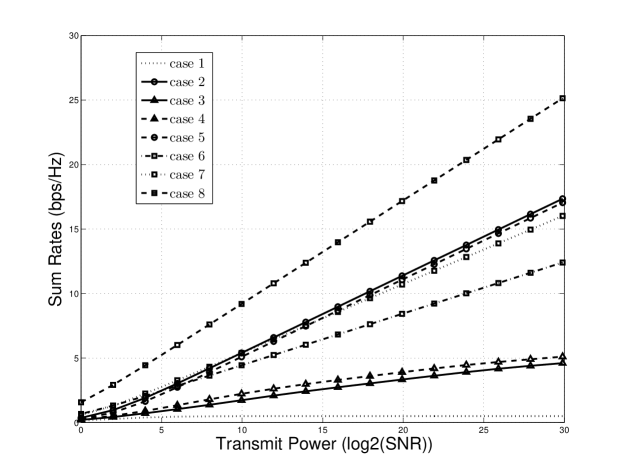
Figure 4: Numerical Results of the RCRM method in Time-Extended Single Antenna Channels (8 cases configured as in Table II)

Numerical results for the above 8 cases in Table II are illustrated in Fig. 4. Case 1 shows an equivalent interference channel as in (2) without any interference alignment design, so that the sum rate deteriorates in high SNR and the achieved DoF is 0. Case 2 shows that process 2 uses the rank minimization method to design $\{\mathrm{G}_{l}\}$ to achieve IA and obtain DoF. Case 3 shows that process 3 uses the leakage minimization method to design $\mathrm{V}_{i}$, $\mathrm{U}_{j}$ to achieves IA as well, but obtaining lower DoF. Case 4 attempts to additionally optimize $\mathrm{V}_{i}$, $\mathrm{U}_{j}$ by leakage minimization on the basis of process 2, however the DoF is reduced to the same level of process 3. The reason is the IA structure formed by relay coding using rank minimization is destroyed, due to the inseparable inter-relationships of relay coding variables as shown in (42). Case 5 shows that process 5 takes an additional step to optimize $\{\mathrm{G}_{l}\}$ using rank minimization method on the basis of process 3. Notice the DoF rises to the same level of process 2, which means the step of relay coding plays the key role in achieving interference alignment. Finally, compare the cases 6, 7 and 8 with case 2. Case 6 shows that when the number of users increase from 3 to 4, interference alignment is no longer feasible. So that less concurrent streams are allowed, i.e. $d$ is reduced from $4$ to $d=2$ to resume IA. Case 7 shows that when the number of users increase to 4, while maintaining the same number of streams as case 2, IA could be still feasible if we increase the time extension length from $T=10$ to $T=15$. However the DoF is yet not increased along with the number of streams, because time extension should be considered resulting in $\text{DoF}=d/T$. So that in case 8, in order to obtain the same number of DoF per user as in case 2, the issue is settled by increasing the number of relays from $L=5$ to $L=10$.

VI-C Applying Novel Relay Coding to Diverse General MIMO Relay Channels

The novel application of rank constrained rank minimization (RCRM) method is proved to be very effective in the relay coding of the $K$-pair time-extended single antenna networks. Furthermore, it is natural to think of extending this idea to more general and realistic scenarios. Network with all nodes equipped with multiple antennas (i.e. MIMO networks) are usually investigated in other works [9, 5]. It is in general hard to design beamforming to mitigate and align interference with conventional optimization techniques. For example, the end-to-end sum-rate maximization problem is non-convex and NP-hard, and implicit MSE(minimum square error) metric and the interference pricing method are considered to obtain sub-optimal solutions [9, 5]. RCRM method is a promising efficient approach to deal with such MIMO interference channels [21, 22]. It is yet non-trivial to apply the RCRM method to MIMO interference channels with relays, where the convexity for relay coding is an issue. Anyhow, the novel approach to apply RCRM in MIMO relay networks provides an simple accessible way.

The following work focuses on general MIMO relay networks without any time symbol extensions. Although it is usually infeasible for MIMO networks to obtain 1/2 DoF for every user by interference alignment [25], the idea of suppressing interference subspace dimension could be still used to obtain high DoF, which captures the key value of interference alignment at high SNR. While RCRM method provides such a measure to minimize the subspace dimension to obtain suboptimal DoF through convex approximation [21, 22]. The RCRM method is non-trivially extended in this work to apply to relay-connected MIMO networks. So that relay coding is involved and designed along with precoding at source and destination nodes, which reflects the strategy of coding in the middle [20].

Moreover, this novel design is further found to be naturally applicable to a wide range of typical relay networks, which are originally hard to analyze and solve. These scenarios include MIMO relay channel, MIMO two-way relay channel, MIMO Y channel, and MIMO multi-hop relay channel.

VI-C1 MIMO Relay Channel

MIMO relay channel exactly means a two-hop interference channel with half-duplex relays and a two-stage transmission procedure. Consider the model in Fig. 2. There are $K$ sources denoted from $I_{1}$ to $I_{K}$; $K$ destinations denoted from $J_{1}$ to $J_{K}$; $L$ relays denoted from $R_{1}$ to $R_{L}$. All nodes are set to be equipped with multiple antennas. $I_{i}$ has $M_{\xi}$ antennas, $\forall i\in\mathcal{K}$; $R_{l}$ has $M_{\chi}$ antennas, $\forall l\in\mathcal{L}$; $J_{j}$ has $M_{\omega}$ antennas, $\forall j\in\mathcal{K}$. All the channels are constant. $\mathrm{H}_{R_{l}I_{i}}$ and $\mathrm{H}_{J_{j}R_{l}}$ as channels from $I_{i}$ to $R_{l}$ and from $R_{l}$ to $J_{j}$ respectively. $\mathrm{H}_{R_{l}I_{i}}\in\mathbb{C}^{M_{\chi}\times M_{\xi}}$ and $\mathrm{H}_{J_{j}R_{l}}\in\mathbb{C}^{M_{\omega}\times M_{\chi}}$. Then the equivalent channel $\Theta_{ji}\in\mathbb{C}^{M_{\omega}\times M_{\xi}}$ is expressed as:

$$\Theta_{ji}=\sum_{l=1}^{L}\mathrm{H}_{J_{j}R_{l}}\mathrm{G}_{l}\mathrm{H}_{R_{l}I_{i}}$$ (48)

For each user $k$, $I_{k}$ transmits $d$ streams to $J_{k}$. So that set $\mathrm{V}_{i}\in\mathbb{C}^{M_{\xi}\times d}$ as the precoding matrix at source $I_{i}$; $\mathrm{G}_{l}\in\mathbb{C}^{M_{\chi}\times M_{\chi}}$ as the network coding matrix at relay $R_{l}$; $\mathrm{U}_{j}\in\mathbb{C}^{M_{\omega}\times d}$ as the receive filter matrix at destination $J_{j}$.

The procedure to apply RCRM method in this MIMO relay network is the same as above in the time-extended single antenna network. The objective function and feasible set are in the same expressions of (45) and (46). The final problem is also in the expression of (47). It is necessary to prove the convexity of the problem in MIMO relay networks by following lemma 8 and lemma 9.

Lemma 8

The objective function (45) for MIMO relay networks is convex regarding $\{\mathrm{G}_{l}\}_{l=1}^{L}$.

Proof: [36, §3.2.2] indicates the operation of composition with an affine mapping preserves convexity or concavity of functions. Suppose $f:\mathbb{R}^{n}\rightarrow\mathbb{R}$, $A\in\mathbb{R}^{n\times m}$, and $b\in\mathbb{R}^{n}$. Define $g:\mathbb{R}^{m}\rightarrow\mathbb{R}$ as $g(x)=f(Ax+b)$, with $\mathbf{dom}g=\{x|Ax+b\in\mathbf{dom}f\}$. Then if $f$ is convex, so is $g$.

Extract all ${M_{\chi}}^{2}L$ elements from all $\mathrm{G}_{l}$ as $\mathcal{G}\in\mathbb{C}^{{M_{\chi}}^{2}L\times 1}$; extract all $d(K-1)dK$ elements from all $\mathcal{J}_{j}$ as $\mathcal{F}\in\mathbb{C}^{d^{2}(K-1)K\times 1}$. According to (48) and (42), obtain that $\mathcal{F}=\mathcal{W}\mathcal{G}$, where $\mathcal{W}\in\mathbb{C}^{d^{2}(K-1)K\times{M_{\chi}}^{2}L}$ is composed of elements from $\{\mathrm{U}_{j}\}$, $\{\mathrm{V}_{i}\}$, $\{\mathrm{H}_{J_{j}R_{l}}\}$, $\{\mathrm{H}_{R_{l}I_{i}}\}$. Express $\mathcal{F}$, $\mathcal{W}$, $\mathcal{G}$ in complex domain to equivalent $\mathcal{F}_{\mathbb{R}}$, $\mathcal{W}_{\mathbb{R}}$ (transformation via matrix operations), $\mathcal{G}_{\mathbb{R}}$ in real domain, so that $\mathcal{F}_{\mathbb{R}}=\mathcal{W}_{\mathbb{R}}\mathcal{G}_{\mathbb{R}}$, where $\mathcal{G}_{\mathbb{R}}\in\mathbb{C}^{2{M_{\chi}}^{2}L\times 1}$, $\mathcal{F}_{\mathbb{R}}\in\mathbb{C}^{2d^{2}(K-1)K\times 1}$, $\mathcal{W}_{\mathbb{R}}\in\mathbb{C}^{2d^{2}(K-1)K\times 2{M_{\chi}}^{2}L}$. So $\mathcal{F}_{\mathbb{R}}$ is an affine mapping from $\mathcal{G}_{\mathbb{R}}$. [21] concludes (45) is convex regarding $\mathcal{F}_{\mathbb{R}}$, therefore (45) is also convex regarding $\mathcal{G}_{\mathbb{R}}$, i.e. regarding $\{\mathrm{G}_{l}\}_{l=1}^{L}$.  $\square$

Lemma 9

The feasible set (46) for MIMO relay networks is convex regarding $\{\mathrm{G}_{l}\}_{l=1}^{L}$.

Proof: [36, §2.3] indicates that affine functions preserve convexity of sets, or allow us to construct convex sets from others. $S\subseteq\mathbb{R}^{n}$ is a convex set. If $f:\mathbb{R}^{k}\rightarrow\mathbb{R}^{n}$ is affine, i.e. $f(x)=Ax+b$, where $A\in\mathbb{R}^{n\times k}$ and $b\in\mathbb{R}^{n}$, the inverse image of $S$ under $f$: $f^{-1}(S)=\{x|f(x)\in S\}$, is convex.

Similar to Lemma 8, extract elements from $\{\mathcal{S}_{j}\}$, $\{\mathrm{G}_{l}\}$ as $\mathcal{F}_{\mathbb{R}}$, $\mathcal{G}_{\mathbb{R}}$ in real domain. According to (48) and (42), $\mathcal{F}_{\mathbb{R}}=\mathcal{W}_{\mathbb{R}}\mathcal{G}_{\mathbb{R}}$, where $\mathcal{F}_{\mathbb{R}}$ is composed of elements from $\{\mathrm{U}_{j}\}$, $\{\mathrm{V}_{i}\}$, $\{\mathrm{H}_{J_{j}R_{l}}\}$, $\{H_{R_{l}I_{i}}\}$. [21] concludes that feasible set of $\mathcal{F}_{\mathbb{R}}$ under constraint (46) is convex, so that the feasible set of $\mathcal{G}_{\mathbb{R}}$ as the inverse image of $\mathcal{S}_{\mathbb{R}}$ is also convex, i.e. the feasible set of $\{\mathrm{G}_{l}\}_{l=1}^{L}$ is convex.

$\square$

Iterative RCRM algorithm for MIMO relay networks: Since lemma 8 and lemma 9 prove that (47) is a typical convex optimization regarding $\{\mathrm{G}_{l}\}$ for MIMO relay network, as well as regarding $\{\mathrm{U}_{j}\}$ and $\{\mathrm{V}_{i}\}$. Then the optimization problem could be proceeded in an iterative manner, regarding $\{\mathrm{V}_{i}\}$, $\{\mathrm{G}_{l}\}$, $\{\mathrm{U}_{j}\}$, until convergence. At every step, the objective function (45) is non-increasing so that convergence is guaranteed. Compared with the algorithms relating to mean squared error (MSE) and sum rate as in [9], this algorithm directly optimizes DoF for high SNR for the MIMO relay network.

VI-C2 MIMO Two-Way Relay Channel

Consider the $K$-pair two-way (bidirectional) relay MIMO interference channel as in [38]. The model is also as shown in Fig. 2. All $I_{k}$ and $J_{k}$ nodes are both sources and destinations, i.e. each $I_{k}$ exchanges data with its partner node $J_{k}$ via intermediate relaying nodes $R_{1},R_{2},\ldots,R_{L}$. The whole procedure are three steps: uplink, forward, downlink. In uplink step, all end nodes $I_{k}$ and $J_{k}$ simultaneously transmit data towards relay nodes $R_{1},R_{2},\ldots,R_{L}$; in forward step, relay node $R_{l}$ filters its received signal $\mathrm{Y}_{R_{l}}$ through a forwarding filter $\mathrm{G}_{l}$; in downlink step, relay nodes $R_{1},R_{2},\ldots,R_{L}$ broadcast network-coded combined signal to all end nodes $I_{k}$ and $J_{k}$. Denote $\mathrm{H}_{R_{l}I_{i}}$, $\mathrm{H}_{I_{i}R_{l}}$, $\mathrm{H}_{J_{j}R_{l}}$ and $\mathrm{H}_{R_{l}J_{j}}$ as channels from $I_{i}$ to $R_{l}$, $R_{l}$ to $I_{i}$, $R_{l}$ to $J_{j}$ and $J_{j}$ to $R_{l}$, respectively. $\mathrm{H}_{R_{l}I_{i}}\in\mathbb{C}^{M_{\chi}\times M_{\xi}}$, $\mathrm{H}_{I_{i}R_{l}}\in\mathbb{C}^{M_{\xi}\times M_{\chi}}$, $\mathrm{H}_{J_{j}R_{l}}\in\mathbb{C}^{M_{\omega}\times M_{\chi}}$, $\mathrm{H}_{R_{l}J_{j}}\in\mathbb{C}^{M_{\chi}\times M_{\omega}}$. Although it does not affect our scheme, notice the downlink channel is reciprocal to the uplink channel, i.e. $\mathrm{H}_{R_{l}I_{i}}=\mathrm{H}_{I_{i}R_{l}}^{{\dagger}}$, $\mathrm{H}_{J_{j}R_{l}}=\mathrm{H}_{R_{l}J_{j}}^{{\dagger}}$.

Then the received signals $\mathrm{Y}_{J_{k}}$ and $\mathrm{Y}_{I_{k}}$ at $J_{k}$ and $I_{k}$ after self interference cancellation (also ignore noise term) are presented as:

$$\mathrm{Y}_{J_{k}} =\sum_{l=1}^{L}\mathrm{H}_{J_{k}R_{l}}\mathrm{G}_{l}\big{(}\sum_{i=1}^{K}\mathrm{H}_{R_{l}I_{i}}\mathrm{V}_{I_{i}}\mathrm{X}_{I_{i}}+\sum_{j=1,j\neq k}^{K}\mathrm{H}_{R_{l}J_{j}}\mathrm{V}_{J_{j}}\mathrm{X}_{J_{j}}\big{)}$$ (49)

$$=\Phi_{J_{k}I_{k}}\mathrm{V}_{I_{k}}\mathrm{X}_{I_{k}}+\sum_{i=1,i\neq k}^{K}\Phi_{J_{k}I_{i}}\mathrm{V}_{I_{i}}\mathrm{X}_{I_{i}}+\sum_{j=1,j\neq k}^{K}\Phi_{J_{k}J_{j}}\mathrm{V}_{J_{j}}\mathrm{X}_{J_{j}}$$

where $$\ \ \Phi_{J_{k}I_{i}}=\sum_{l=1}^{L}\mathrm{H}_{J_{k}R_{l}}\mathrm{G}_{l}\mathrm{H}_{R_{l}I_{i}}\ \ \text{and}\ \ \Phi_{J_{k}J_{j}}=\sum_{l=1}^{L}\mathrm{H}_{J_{k}R_{l}}\mathrm{G}_{l}\mathrm{H}_{R_{l}J_{j}}$$

$$\mathrm{Y}_{I_{k}} =\sum_{l=1}^{L}\mathrm{H}_{I_{k}R_{l}}\mathrm{G}_{l}\big{(}\sum_{i=1,i\neq k}^{K}\mathrm{H}_{R_{l}I_{i}}\mathrm{V}_{I_{i}}\mathrm{X}_{I_{i}}+\sum_{j=1}^{K}\mathrm{H}_{R_{l}J_{j}}\mathrm{V}_{J_{j}}\mathrm{X}_{J_{j}}\big{)}$$

$$=\Phi_{I_{k}J_{k}}\mathrm{V}_{J_{k}}\mathrm{X}_{J_{k}}+\sum_{i=1,i\neq k}^{K}\Phi_{I_{k}I_{i}}\mathrm{V}_{I_{i}}\mathrm{X}_{I_{i}}+\sum_{j=1,j\neq k}^{K}\Phi_{I_{k}J_{j}}\mathrm{V}_{J_{j}}\mathrm{X}_{J_{j}}$$

where $$\ \ \Phi_{I_{k}I_{i}}=\sum_{l=1}^{L}\mathrm{H}_{I_{k}R_{l}}\mathrm{G}_{l}\mathrm{H}_{R_{l}I_{i}}\ \ \text{and}\ \ \ \Phi_{I_{k}J_{j}}=\sum_{l=1}^{L}\mathrm{H}_{I_{k}R_{l}}\mathrm{G}_{l}\mathrm{H}_{R_{l}J_{j}}$$

(49) shows the model is equivalent to $2K$ users transmitting in pairs, and there are $(2K)^{2}$ equivalent channels between transmitters and receivers which are $\{\Phi_{J_{k}I_{i}}\}$, $\{\Phi_{J_{k}J_{j}}\}$, $\{\Phi_{I_{k}I_{i}}\}$, $\{\Phi_{I_{k}J_{j}}\}$. The coding procedure is just the same as the case of MIMO relay networks. We could obtain the same RCRM problem for MIMO two-way relay networks as in (47), which is proved to be a convex optimization through the following similar lemmas.

Lemma 10

For MIMO two-way relay networks as in (49), the corresponding rank minimization objective function (45) is convex regarding $\{\mathrm{G}_{l}\}_{l=1}^{L}$ .

Proof: Proof is similar to lemma 8.  $\square$

Lemma 11

For MIMO two-way relay networks as in (49), the corresponding rank constrained feasible set (46) is convex regarding $\{\mathrm{G}_{l}\}_{l=1}^{L}$.

Proof: Proof is similar to lemma 9.  $\square$

VI-C3 MIMO Y Channel

Consider MIMO Y channel as in [39]. The model is also illustrated by Fig. 2. The network only has three user nodes which are set as $I_{1}$, $I_{2}$, $I_{3}$, and one relay node set as $R_{1}$. Each user intends to convey independent messages for the other two users via the relay, while receiving two independent messages from the other two users. The transmission has two phases. First phase is the multiple-access channel (MAC) phase, when all users transmit to the relay; second phase is the broadcast (BC) phase, when the relay generates new transmitting signals and send to all users. Denote $\mathrm{V}_{I_{i}}^{[I_{k}]}$ and $\mathrm{X}_{I_{i}}^{[I_{k}]}$ as the precoding matrix and input data from $I_{i}$ to $I_{k}$.

Then the received signals $\mathrm{Y}_{I_{k}}$ at $I_{k}$ after self interference cancellation and $\mathrm{Y}_{R_{1}}$ at $R_{1}$ (both ignore noise terms) are:

$$\mathrm{Y}_{R_{1}}=\mathrm{H}_{R_{1}I_{1}}\big{(}\mathrm{V}_{I_{1}}^{[I_{2}]}\mathrm{X}_{I_{1}}^{[I_{2}]}+\mathrm{V}_{I_{1}}^{[I_{3}]}\mathrm{X}_{I_{1}}^{[I_{3}]}\big{)}$$ (50)

$$\hskip 25.60747pt+\mathrm{H}_{R_{1}I_{2}}\big{(}\mathrm{V}_{I_{2}}^{[I_{3}]}\mathrm{X}_{I_{2}}^{[I_{3}]}+\mathrm{V}_{I_{2}}^{[I_{1}]}\mathrm{X}_{I_{2}}^{[I_{1}]}\big{)}$$

$$\hskip 25.60747pt+\mathrm{H}_{R_{1}I_{3}}\big{(}\mathrm{V}_{I_{3}}^{[I_{1}]}\mathrm{X}_{I_{3}}^{[I_{1}]}+\mathrm{V}_{I_{3}}^{[I_{1}]}\mathrm{X}_{I_{3}}^{[I_{1}]}\big{)}$$

$$\mathrm{Y}_{I_{k}}=\mathrm{H}_{I_{k}R_{1}}\mathrm{G}_{1}\mathrm{Y}_{R_{1}}$$

so that:

$$\mathrm{Y}_{I_{1}}=\big{(}\mathrm{H}_{I_{1}R_{1}}\mathrm{G}_{1}\mathrm{H}_{R_{1}I_{2}}\big{)}\mathrm{V}_{I_{2}}^{[I_{1}]}\mathrm{X}_{I_{2}}^{[I_{1}]}+\big{(}\mathrm{H}_{I_{1}R_{1}}\mathrm{G}_{1}\mathrm{H}_{R_{1}I_{3}}\big{)}\mathrm{V}_{I_{3}}^{[I_{1}]}\mathrm{X}_{I_{3}}^{[I_{1}]}$$

$$\mathrm{Y}_{I_{2}}=\big{(}\mathrm{H}_{I_{2}R_{1}}\mathrm{G}_{1}\mathrm{H}_{R_{1}I_{3}}\big{)}\mathrm{V}_{I_{3}}^{[I_{2}]}\mathrm{X}_{I_{3}}^{[I_{2}]}+\big{(}\mathrm{H}_{I_{2}R_{1}}\mathrm{G}_{1}\mathrm{H}_{R_{1}I_{1}}\big{)}\mathrm{V}_{I_{1}}^{[I_{2}]}\mathrm{X}_{I_{1}}^{[I_{2}]}$$

$$\mathrm{Y}_{I_{3}}=\big{(}\mathrm{H}_{I_{3}R_{1}}\mathrm{G}_{1}\mathrm{H}_{R_{1}I_{1}}\big{)}\mathrm{V}_{I_{1}}^{[I_{3}]}\mathrm{X}_{I_{1}}^{[I_{3}]}+\big{(}\mathrm{H}_{I_{3}R_{1}}\mathrm{G}_{1}\mathrm{H}_{R_{1}I_{2}}\big{)}\mathrm{V}_{I_{2}}^{[I_{3}]}\mathrm{X}_{I_{2}}^{[I_{3}]}$$

(50) shows the model is equivalent to $6$ pairs of users transmitting on $36$ equivalent channels. We could obtain the same RCRM problem as in (47) for MIMO Y channel. It is proved to be convex through the following similar lemmas.

Lemma 12

For the MIMO Y channel as in (50), the corresponding rank minimization objective function (45) is convex regarding $\{\mathrm{G}_{l}\}_{l=1}^{L}$ .

Proof: Proof is similar to lemma 8.  $\square$

Lemma 13

For the MIMO Y channel as in (50), the corresponding rank constrained feasible set (46) is convex regarding $\{\mathrm{G}_{l}\}_{l=1}^{L}$.

Proof: Proof is similar to lemma 9.  $\square$

Compared with [39], the analytical signal space alignment and network-coding-aware interference nulling beamforming scheme is complicated to be implemented and hard to adapt to changes of structure. While this RCRM method is a direct solution to form efficient and robust coding.

VI-C4 MIMO Multi-hop Relay Channel

Consider MIMO interference channels with multi-hop relays as in [3, 18]. The model in Fig. 2 needs to be modified. There are $M$ layers of parallel relaying nodes between sources and destinations in the network. Denote the $m$-th layer’s nodes as $R_{1,m},R_{2,m},\ldots,R_{L,m}$, and the corresponding filter matrices are $\mathrm{G}_{1,m},\mathrm{G}_{2,m},\ldots,\mathrm{G}_{L,m}$. The channels are denoted as $\mathrm{H}_{J_{j}R_{l,M}}$ from $M$-th layer of relays to destination $J_{j}$, $\mathrm{H}_{R_{l,m}R_{l,m-1}}$ from $(m-1)$-th layer of relays to $m$-th layer of relays, $\mathrm{H}_{R_{l,1}I_{i}}$ from source $I_{i}$ to $1$-st layer of relays.

For simplicity, only assume there are two layers of relays. $\mathrm{G}_{q,1}$ is the filter at $q$-th relay in first layer and $\mathrm{G}_{p,2}$ is the filter at $p$-th relay in second layer. $\mathrm{H}_{R_{q,1}I_{i}}$, $\mathrm{H}_{R_{p,2}R_{q,1}}$, and $\mathrm{H}_{J_{j}R_{p,2}}$ are channels from source $I_{i}$ to relay $R_{q,1}$, from relay $R_{q,1}$ to relay $R_{p,2}$, and from relay $R_{p,2}$ to destination $J_{j}$. Then the received signal $\mathrm{Y}_{J_{j}}$ at $J_{j}$ is:

$$\mathrm{Y}_{J_{j}} =\sum_{p=1}^{L}\mathrm{H}_{J_{j}R_{p,2}}\mathrm{G}_{p,2}\sum_{q=1}^{L}\mathrm{H}_{R_{p,2}R_{q,1}}\mathrm{G}_{q,1}\sum_{i=1}^{K}\mathrm{H}_{R_{q,1}I_{i}}\mathrm{V}_{I_{i}}\mathrm{X}_{I_{i}}$$ (51)

The equivalent channel from $I_{i}$ to $J_{j}$ is:

$\Phi_{J_{j}I_{i}}=\sum_{p=1}^{L}\mathrm{H}_{J_{j}R_{p,2}}\mathrm{G}_{p,2}\sum_{q=1}^{L}\mathrm{H}_{R_{p,2}R_{q,1}}\mathrm{G}_{q,1}\mathrm{H}_{R_{q,1}I_{i}}$

Iterative algorithms layer by layer: At each step, choose one layer of relays as the coding variables, then we could obtain the same RCRM problem as in (47). The whole algorithm is convergent, since the objective function maintains the same all the time. It is proved to be a convex optimization problem through following similar lemmas.

Lemma 14

For the MIMO interference channels with multi-hop relays as in (51), the corresponding rank minimization objective function (45) is convex regarding $\{\mathrm{G}_{l,m}\}_{(l,m)=(1,1)}^{(L,M)}$.

Proof: Proof is similar to lemma 8.  $\square$

Lemma 15

For the MIMO interference channels with multi-hop relays as in (51), the corresponding rank constrained feasible set (46) is convex regarding $\{\mathrm{G}_{l,m}\}_{(l,m)=(1,1)}^{(L,M)}$.

Proof: Proof is similar to lemma 9.  $\square$

In summary, MIMO interference channels with multi-hop relays are generally hard to have either analytical or numerical solutions [3, 18]. While this novel RCRM based algorithm provides a robust and universal solution.

VI-C5 Numerical Results for Diverse MIMO Relay Networks

All the numerical results are shown in Fig. 5. The above four scenarios of MIMO relay channel, MIMO two-way relay channel, MIMO Y channel and MIMO multi-hop channel are denoted as case 1, case 2, case 3, and case 4, respectively. Configure the four cases as shown in Table III. In case 3, ’1$\times$2’ means 2 separate streams at one user in the MIMO Y channel. In case 4, ’3$\times$2’ means 2 layers of relays (3 relay in each layer) in the multi-hop relay network.

Case	$K$	$L$	$M_{\xi}$	$M_{\chi}$	$M_{\omega}$	d
1	3	3	10	5	10	2
2	3	3	10	10	10	2
3	3	1	10	10	10	1$\times$2
4	3	3$\times$2	10	5	10	2

TABLE III: Configurations of 4 cases of MIMO relay networks

Simulation has been done with the software tool CVX [37]. In Fig. 5, ’Ref’ means random coding as a reference for the 4 kinds of MIMO relay networks, which obviously obtain 0 DoF. While ’Opt’ means results with the IA coding design, which shows that DoF is well obtained. So that the novel application of RCRM method in relay networks successfully implements interference alignment in typical scenarios. Case 2 has the largest DoF because it has bidirectional transmissions. In case 3, MIMO Y channel transmits 2 datastreams for each user, however there is only 1 DoF for each virtual port. In case 4, multi-hop relays relaxe the requirements for individual relays in each layer to maitain high DoF. In summary, this novel relay coding design successfully implements interference alignment in above relay-involved scenarios as a effective universal solution.

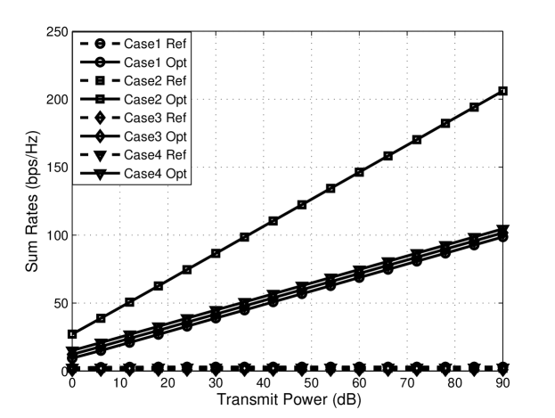
Figure 5: Rates of 4 cases of MIMO relay networks (4 cases as configured in Table III before and after relay coding optimization)

VII Conclusion

This work considers two strategies in which a finite number of relays can be employed to achieve IA in a $K$-pair interference network. In the coding-at-the-edge strategy, in the single antenna constant channel, relays can be used with time extension techniques to produce equivalent channels where standard IA schemes are applicable. However, at least two relays are proved to be required to produce channel randomness, which is a necessity for all kinds of IA schemes to be achievable. Novel precoding schemes with double-layered symbol extensions could also be used to investigate the issue of constant channels. In the coding-in-the-middle strategy, as a universal numerical approach for diverse general MIMO networks with relays, relay coding can be designed as an optimization problem to minimize the rank of the interference subspace. Efficient and robust algorithms are proposed.

References

• [1] V. Cadambe and S. Jafar, “Interference alignment and degrees of freedom of the K-user interference channel,” IEEE Transactions on Information Theory, vol. 54, no. 8, pp. 3425–3441, Aug. 2008.
• [2] V. R. Cadambe and S. A. Jafar, “Can feedback, cooperation, relays and full duplex operation increase the degrees of freedom of wireless networks ?” in IEEE International Symposium on Information Theory, Toronto, Canada, July 2008, pp. 1263–1267.
• [3] S. W. Jeon, S. Y. Chung, and S. A. Jafar. (2009, October) Degrees of freedom of multi-source relay networks. arXiv:0910.3275v1.
• [4] M. Plainchault, N. Gresset, and G. R. B. Othman, “Interference relay channel with precoded dynamic decode and forward protocols,” in IEEE Global Communications Conference (GLOBECOM), Houston, TX, USA, December 2011.
• [5] K. T. Trung and R. W. H. Jr., “Relay beamforming using interference pricing for the two-hop interference channel,” in IEEE Global Communications Conference (GLOBECOM), Houston, TX, USA, December 2011.
• [6] R. Wang and M. Tao, “Linear precoding designs for amplify-and-forward multiuser two-way relay systems,” in IEEE Global Communications Conference (GLOBECOM), Houston, TX, USA, December 2011.
• [7] C. Wang, H. Farhadi, and M. Skoglund, “On the degrees of freedom of parallel relay networks,” in IEEE Global Communications Conference (GLOBECOM), Miami, Florida, USA, December 2010.
• [8] B. Bai, W. Chen, K. B. Letaief, and Z. Cao, “Optimal relay selection and channel allocation for multi-user analog two-way relay systems,” in IEEE Global Communications Conference (GLOBECOM), Houston, TX, USA, December 2011.
• [9] K. T. Truong and R. W. H. Jr., “Interference alignment for multiple-antenna amplify-and-forward relay interference channel,” in 46th Annual Asilomar Conference on Signals, Systems, and Computers, Pacific Grove, California, USA, November 2011.
• [10] R. S. Ganesan, T. Weber, and A. Klein, “Interference alignment in multi-user two way relay networks,” in IEEE Vehicular Technology Conference (VTC), Yokohama, May 2011.
• [11] C. Huang, M. Zeng, and S. Cui, “Achievable rates of two-hop interference networks with conferencing relays,” in IEEE Global Communications Conference (GLOBECOM), Houston, TX, USA, December 2011.
• [12] D.-S. Jin, J. S. No, and D. J. Shin, “Interference alignment aided by relays for the quasi-static X channel,” in IEEE International Symposium on Information Theory (ISIT), St. Petersburg, Russia, August 2011, pp. 2652–2656.
• [13] B. Nazer, M. Gastpar, S. A. Jafar, and S. Vishwanath, “Ergodic interference alignment,” in IEEE International Symposium on Information Theory (ISIT), 28 2009-July 3 2009, pp. 1769–1773.
• [14] H. Ning, C. Ling, and K. K. Leung, “Relay-aided interference alignment: feasibility conditions and algorithm,” in IEEE International Symposium on Information Theory (ISIT), Austin, Texas, U.S.A., June 2010, pp. 390–394.
• [15] B. Nourani, S. A. Motahari, and A. K. Khandani, “Relay-aided interference alignment for the quasi-static X channel,” in IEEE International Symposium on Information Theory (ISIT), Seoul, Korea, July 2009, pp. 1764–1768.
• [16] ——, “Relay-aided interference alignment for the quasi-static interference channel,” in IEEE International Symposium on Information Theory, Austin, Texas, USA, June 2010, pp. 405–409.
• [17] S. Chen and R. S. Cheng, “Achieve the degrees of freedom of K-user MIMO interference channel with a MIMO relay,” in IEEE Global Communications Conference (GLOBECOM), Miami, Florida, USA, December 2010.
• [18] S.-W. Jeon, S.-Y. Chung, and S. A. Jafar, “Degrees of freedom region of a class of multi-source Gaussian relay networks,” IEEE Transactions on Information Theory, vol. 57, no. 5, pp. 3032–3044, May 2011.
• [19] T. Gou, S. A. Jafar, S. W. Jeon, and S. Y. Chung. (2010, December) Aligned interference neutralization and the degrees of freedom of the 2x2x2 interference channel. arXiv:1012.2350v1.
• [20] A. Ramakrishnan, A. Das, H. Maleki, A. Markopoulou, S. Jafar, and S. Vishwanath, “Network coding for three unicast sessions: Interference alignment approaches,” in 48th Annual Allerton Conference on Communication, Control, and Computing, Allerton, USA, September 2010, pp. 1054–1061.
• [21] D. S. Papailiopoulos and A. G. Dimakis. (2010, December) Interference alignment as a rank constrained rank minimization. arXiv:1010.0476v2.
• [22] ——, “Interference alignment as a rank constrained rank minimization,” in IEEE Global Communications Conference, Miami, USA, December 2010.
• [23] K. Gomadam, V. Cadambe, and S. Jafar, “Approaching the capacity of wireless networks through distributed interference alignment,” in IEEE Global Telecommunications Conference, 30 2008-Dec. 4 2008, pp. 1–6.
• [24] A. S. Avestimehr, S. N. Diggavi, and D. N. C. Tse, “A deterministic approach to wireless relay networks,” Oct 2007. [Online]. Available: http://arxiv.org/abs/0710.3777
• [25] C. M. Yetis, T. Gou, S. A. Jafar, and A. H. Kayran, “On feasibility of interference alignment in MIMO interference networks,” IEEE Transactions on Signal Processing, vol. 58, no. 9, pp. 4771–4782, September 2010.
• [26] H. Zhou, D. Wilcox, T. Ratnarajah, and M. Sellathurai, “Single antenna interference alignment for finite relay networks,” in 19th International Conference on Systems, Signals and Image Processing (IWSSIP), Vienna, Austria, April 2012.
• [27] H. Zhou, T. Ratnarajah, M. Sellathurai, and D. Wilcox, “On achievable schemes of interference alignment in constant channels via finite amplify-and-forward relays,” 2012, to be submitted.
• [28] S. W. Choi, S. A. Jafar, and S.-Y. Chung, “On the beamforming design for efficient interference alignment,” IEEE Communications Letters, vol. 13, no. 11, pp. 847–649, November 2009.
• [29] A. S. Motahari, S. Oveis-Gharan, M.-A. Maddah-Ali, and A. K. Khandani. (2009, November) Real interference alignment: exploiting the potential of single antenna systems. arXiv:0908.2282v2. [Online]. Available: http://arxiv.org/abs/0908.2282v2
• [30] M. A. Maddah-Ali. (2009, October) On the degrees of freedom of the compound mimo broadcast channels with finite states. arXiv:0909.5006.
• [31] V. Cadambe, S. A. Jafar, and C. Wang, “Interference alignment with asymmetric complex signaling - settling the Høst-Madsen-Nosratinia conjecture,” IEEE Transactions on Information Theory, vol. 56, no. 9, pp. 4552–4565, September 2010.
• [32] A. Høst-Madsen and A. Nosratinia, “The multiplexing gain of wireless networks,” in International Symposium on Information Theory, Sept. 2005, pp. 2065–2069.
• [33] V. R. Cadambe and S. A. Jafar, “Interference alignment and spatial degrees of freedom for the K user interference channel,” in IEEE International Conference on Communications, May 2008, pp. 971–975.
• [34] B. A. Cetiner, N. Biyikli, B. S. Yildirim, and Y. Damgaci, “Nano-electromechanical switches for reconfigurable antennas,” Microwave and Optical Technology Letters, vol. 52, no. 1, pp. 64–69, November 2009.
• [35] T. Gou, C. Wang, and S. A. Jafar, “Aiming perfectly in the dark-blind interference alignment through staggered antenna switching,” IEEE Transactions on Signal Processing, vol. 59, no. 6, pp. 2734–2744, June 2011.
• [36] S. Boyd and L. Vandenberghe, Convex optimization.   Cambridge University Press, 2004.
• [37] M. Grant and S. Boyd. (2009, June) Cvx: Matlab software for disciplined convex programming. http://stanford.edu/ boyd/cvx.
• [38] T. K. Akino, M. O. Pun, and P. Orlik, “Network-coded interference alignment in K-pair bidirectional relaying channels,” in IEEE International Conference on Communications (ICC), Kyoto, Japan, June 2011.
• [39] N. Lee, J. bu Lim, and J. Chun, “Degrees of freedom of the MIMO Y channel: signal space alignment for network coding,” IEEE Transactions on Information Theory, vol. 56, no. 7, July 2010.