Correcting gene expression data when neither the unwanted variation nor the factor of interest are observed

Abstract

When dealing with large scale gene expression studies, observations are commonly contaminated by unwanted variation factors such as platforms or batches. Not taking this unwanted variation into account when analyzing the data can lead to spurious associations and to missing important signals. When the analysis is unsupervised, e.g. when the goal is to cluster the samples or to build a corrected version of the dataset — as opposed to the study of an observed factor of interest — taking unwanted variation into account can become a difficult task. The unwanted variation factors may be correlated with the unobserved factor of interest, so that correcting for the former can remove the latter if not done carefully. We show how negative control genes and replicate samples can be used to estimate unwanted variation in gene expression, and discuss how this information can be used to correct the expression data or build estimators for unsupervised problems. The proposed methods are then evaluated on three gene expression datasets. They generally manage to remove unwanted variation without losing the signal of interest and compare favorably to state of the art corrections.

1 Introduction

Over the last few years, microarray-based gene expression studies involving a large number of samples have been carried out (Cardoso et al., 2007; Cancer Genome Atlas Research Network, 2008), with the hope to help understand or predict some particular factors of interest like the prognosis or the subtypes of a cancer. Such large gene expression studies are often carried out over several years, may involve several hospitals or research centers and typically contain some unwanted variation (UV) factors. These factors can arise from technical elements such as batches, different technical platforms or laboratories, or from biological signals which are unrelated to the factor of interest of the study such as heterogeneity in ages or different ethnic groups. They can easily lead to spurious associations. When looking for genes which are differentially expressed between two subtypes of cancer, the observed differential expression of some genes could actually by caused by laboratories if laboratories are partially confounded with subtypes. When doing clustering to identify new subgroups of the disease, one may actually identify any of the UV factors if their effect on gene expression is stronger than the subgroup effect. If one is interested in predicting prognosis, one may actually end up predicting whether the sample was collected at the beginning or at the end of the study because better prognosis patients were accepted at the end of the study. In this case, the classifier obtained would have little value for predicting the prognosis of new patients outside the study. Similar problems arise when doing a meta-analysis, i.e., when trying to combine several smaller studies rather than working on a large heterogeneous study : in a dataset resulting from the merging of several studies the strongest effect one can observe is generally related to the membership of samples to different studies.

A very important objective is therefore to remove these UV factors without losing the factor of interest. The problem can be more or less difficult depending on what is actually considered to be observed and what is not. If both the factor of interest and all the UV factors (say technical batches or different countries) are known, the problem essentially boils down to a linear regression : the expression of each gene is decomposed as an effect of the factor of interest plus an effect of the unwanted variation factor. When the variance of each gene is assumed to be different within each batch, this leads to so-called location and scale adjustments such as used in dChip (Li and Wong, 2003). Johnson et al. (2007) shrink the unwanted variation and variance of all genes within each batch using an empirical Bayes method. This leads to the widely used ComBat method which generally give good performances in this case. Walker et al. (2008) propose a version of ComBat which uses replicate samples to estimate the batch effect. When replicate samples are available an alternative to centering, known as ratio-based method (Luo et al., 2010) is to remove the average of the replicate samples within each batch rather than the average of all samples. Assuming that the factor of interest is associated with the batch, this should ensure that centering the batches does not remove the signal associated with the factor of interest. Note that this procedure is closely related to some of the methods we introduce in this paper.

Of course there is always a risk that some unknown factors also influence the gene expression. Furthermore it is sometimes better when tackling the problem with linear models to consider UV factors which are actually known as unknown. Their effect may be strongly non-linear because they don’t affect all samples the same way or because they interact with other factors, in which cases modeling them as known may give poor results. When the UV factors are modeled as unknown, the problem becomes more difficult because one has to estimate UV factors along with their effects on the genes and that many estimates may explain the data equally well while leading to very different conclusions. ICE (Kang et al., 2008) models unwanted variation as the combination of an observed fixed effect and an unobserved random effect. The covariance of the random effect is taken to be the covariance of the gene expression matrix. The risk of this approach is that some of the signal associated with the signal of interest may be lost because it is included in the covariance of the gene expression matrix. SVA (Leek and Storey, 2007) addresses the problem by first estimating the effect of the factor of interest on each gene then doing factor analysis on the residuals, which intuitively can give good results as long as the UV factors are not too correlated with the factor of interest. Teschendorff et al. (2011) propose a variant of SVA where the factor analysis step is done by independent component analysis (Hyvärinen, 2001) instead of SVD. The same model as Leek and Storey (2007) is considered in a recent contribution of Gagnon-Bartsch and Speed (2012) coined RUV-2, which proposes a general framework to correct for UV in microarray data using negative control genes. These genes are assumed not to be affected by the factor of interest and used to estimate the unwanted variation component of the model. They apply the method to several datasets in an extensive study and show its very good behavior for differential analysis, in particular comparable performances to state of the art methods such as ComBat (Johnson et al., 2007) or SVA (Leek and Storey, 2007). Sun et al. (2012) recently proposed LEAPS, which estimates the parameters of a similar model in two steps : first the effect of unwanted variation is estimated by SVD on the data projected along the factor of interest, then the unwanted variation factors responsible for this effect and the effect of the factor of interest are estimated jointly using an iterative coordinate descent scheme. A sparsity-inducing penalty is added to the effect of the factor of interest in order to make the model identifiable. Yang et al. (2012) adopt a related approach : they also use the sparsity-inducing penalty, do not have the projection step and relax the rank constraint to a trace constraint which makes the problem jointly convex in the unwanted variation and effect of the factor of interest. Listgarten et al. (2010) model the unwanted variation as a random effect term, like ICE. The covariance of the random effect is estimated by iterating between a maximization of the likelihood of the factor of interest (fixed effect) term for a given estimate of the covariance and a maximization of the likelihood of the covariance for a given estimate of the fixed effect term. This is also shown to yield better results than ICE and SVA.

Finally when the factor of interest is not observed, the problem is even more difficult. It can occur if one is interested in unsupervised analyses such as PCA or clustering. Suppose indeed that one wants to use a large study to identify new cancer subtypes. If the study contains several technical batches, includes different platforms or different labs or any unknown factor, the samples may cluster according to one of these factors hence defeating the purpose of using a large set of samples to identify more subtle subtypes. One may also simply want to “clean” a large dataset from its UV without knowing in advance which factors of interest will be studied. Accordingly in the latter case, any knowledgeable person may want to start form the raw data and use the factor of interest once it becomes known to remove UV. Alter et al. (2000); Nielsen et al. (2002) use SVD on gene expression to identify the UV factors without requiring the factor of interest, Price et al. (2006) do so using axes of principal variance observed on SNP data. These approaches may work well in some cases but relies on the prior belief that all UV factors explain more variance than any factor of interest. Furthermore it will fail if the UV factors are too correlated with the factor of interest. If the factor of interest is not observed but the unwanted variation factor is assumed to be an observed batch, an alternative approach is to project the data along the batch factors, equivalently to center the data by batch. This is conceptually similar to using one of the location and scale adjustment methods such as Li and Wong (2003) or Johnson et al. (2007) without specifying the factor of interest. Benito et al. (2004); Marron et al. (2007) propose a distance weighted discrimination (DWD) method which uses a supervised learning algorithm to finds a hyperplane separating two batches and project the data on this hyperplane. As with the dChip and ComBat approaches, assuming that the unwanted variation is a linear function of the observed batch may fail if other unwanted variation factors affect gene expression or if the effect of the batch is a more complicated — possibly non-linear — function, or involves interaction with other factors. In addition, like the SVD approach, these projections may subsequently lead to poor estimation of the factor of interest if it is correlated with the batch effect : if one of the batches contains most of one subtype and the second batch contains most of the other subtype the projection step removes a large part of the subtype signal. Finally, Oncomine (Rhodes et al., 2004b, a, 2007) regroups a large number of gene expression studies which are processed by median centering and normalizing the standard deviation to one for each array. This processing does not explicitly take into account a known unwanted variation factor or try to estimate it. It removes scaling effects, e.g. if one dataset or part of a dataset has larger values than others, but it does not correct for multivariate behaviors such as the linear combination of some genes is larger for some batch. On the other hand, it does not run the risk to remove biological signal of this form.

The contribution of Gagnon-Bartsch and Speed (2012) suggests that negative controls can be used to estimate and remove efficiently sources of unwanted variation. Our objective here is to propose ways to improve estimation in the unsupervised case, i.e, when the factor of interest is not observed. We use a random effect to model unwanted variation. As we discuss in the paper, this choice is crucial to obtain good estimators when the factor of interest is not observed. In this context, two main difficulties arise :

• In the regression case, and assuming the covariance of the random term is known, introducing such a random term simply turns the ordinary least square problem into a generalized least square one for which a closed form solution is also available. For some unsupervised estimation problems — such as clustering — dealing with the random effects can be more difficult : the dedicated algorithm — such as $k$-means — may not apply or adapt easily to the adding of a random effect term. Our first contribution is to discuss general ways of adapting dedicated algorithms to the presence of a random effect term.

• As always when using random effects, a major difficulty is to estimate the covariance of the random term. Following Gagnon-Bartsch and Speed (2012), we can use negative control genes to estimate this covariance, but this amounts to assuming that the expression of these genes is really not influenced by the factor of interest. A second contribution of this paper is to propose new ways to estimate the unwanted variation factors using replicate arrays. Replicate arrays correspond to the same biological sample, but typically differ for some unwanted variation factors. For example in a dataset involving two platforms, some samples could be hybridized on the two platforms. More generally in a large study, some control samples or mixtures of RNAs may be re-hybridized at several times of the study, under different conditions. We still don’t know what the factor of interest is, but we know it takes the same value for all replicates of the same sample. Changes among these replicates are therefore only caused by unwanted variation factors, and we intend to use this fact to help identify and remove this unwanted variation.

A third contribution of this paper is to assess how various correction methods, including the ones we introduce, perform in an unsupervised estimation task on three gene expression datasets subject to unwanted variation. We show that the proposed methods generally allow us to solve the unsupervised estimation problem, with no explicit knowledge of the unwanted variation factors.

Section 2 recalls the model and estimators used in Gagnon-Bartsch and Speed (2012). Section 3 presents our methods addressing the case where the factor of interest is unobserved using a random effect term. We first make the assumption that the unwanted variation factors, or equivalently the covariances of the random terms are known. Section 4 discusses how estimation of this unwanted variation factor can be improved. In Section 5, the performance of the proposed methods are illustrated on three gene expression datasets : the gender data of Vawter et al. (2004) which were already used to evaluate the RUV-2 method of Gagnon-Bartsch and Speed (2012), the TCGA glioblastoma data (Cancer Genome Atlas Research Network, 2008) and MAQC-II data from rat liver and blood (Lobenhofer et al., 2008; Fan et al., 2010). We finish with a discussion in Section 6.

Notation

For any matrix $A\in\mathbb{R}^{m,n}$, $\|A\|_{F}\stackrel{{\scriptstyle\Delta}}{{=}}\left(\sum_{i=1}^{m}\sum_{j=1}^{n}a_{ij}^{2}\right)^{\frac{1}{2}}$ denotes the Frobenius norm of $A$. In addition for a positive definite matrix $B\in\mathbb{R}^{m,m}$ we define $\|A\|_{B}\stackrel{{\scriptstyle\Delta}}{{=}}\|B^{-\frac{1}{2}}A\|_{F}$. We refer to the problem where the factor of interest is observed as the supervised problem, and to the problem where it is unobserved as the unsupervised problem.

2 Existing fixed effect estimators : RUV-2 and naive RUV-2

The RUV (Removal of Unwanted Variation) model used by Gagnon-Bartsch and Speed (2012) was a linear model, with one term representing the effect of the factors of interest on gene expression and another term representing the effect of the unwanted variation factors :

$$Y=X\beta+W\alpha+\varepsilon,$$ (1)

with $Y\in\mathbb{R}^{m\times n}$, $X\in\mathbb{R}^{m\times p}$, $\beta\in\mathbb{R}^{p\times n}$, $W\in\mathbb{R}^{m\times k}$, $\alpha\in\mathbb{R}^{k\times n}$ and $\varepsilon\in\mathbb{R}^{m\times n}$. $Y$ is the observed matrix of expression of $n$ genes for $m$ samples, $X$ represents the $p$ factors of interest, $W$ the $k$ unwanted variation factors and $\varepsilon$ some noise, typically $\varepsilon_{j}\sim\mathcal{N}(0,\sigma^{2}_{\varepsilon}I_{m}),\,j=1,\ldots,n$. Both $\alpha$ and $\beta$ are modeled as fixed, i.e., non-random (Robinson, 1991).

A similar model was also used in Leek and Storey (2007) and Listgarten et al. (2010). The latter used a mixed effect model where $\alpha$ was random. All these methods addressed the supervised problem, i.e., the case where $X$ is an observed factor of interest and the goal is to estimate its effect $\beta$ knowing that some other factors influence gene expression. They differ in the way parameters $\beta$ and $W\alpha$ are estimated. For the sake of clarity, we now recall the approach of Gagnon-Bartsch and Speed (2012) from which our unsupervised estimators are derived.

2.1 Supervised RUV-2

The method of Gagnon-Bartsch and Speed (2012) exploits the fact that some genes are known to be negative controls, i.e., not to be affected by the factor of interest. Formally we suppose that $\beta_{c}=0$ where $\beta_{c}$ is the restriction of $\beta$ to its column in some index $c$ denoting the negative control genes.

The objective in Gagnon-Bartsch and Speed (2012) is to test the hypothesis that $\beta_{j}=0$ for each gene $j$ in order to identify differentially expressed genes. They use an intuitive two-step algorithm coined RUV-2 to estimate $W\alpha$ and $\beta$ :

1. Use the columns of $Y$ corresponding to control genes

   $$Y_{c}=W\alpha_{c}+\varepsilon_{c},$$ (2)

   to estimate $W$. Assuming iid noise $\varepsilon_{j}\sim\mathcal{N}(0,\sigma^{2}_{\varepsilon}I_{m}),\,j\in c$, the $(W\alpha_{c})$ matrix maximizing the likelihood of (2) is $\operatorname*{arg\,min}_{W\alpha_{c},\textrm{rank}W\alpha_{c}\geq k}\|Y_{c}-W\alpha_{c}\|_{F}^{2}$. By the Eckart-Young theorem (Eckart and Young, 1936), this argmin is reached for $\widehat{W\alpha_{c}}=U\Lambda_{k}V^{\top}$, where $Y_{c}=U\Lambda V^{\top}$ is the singular value decomposition (SVD) of $Y_{c}$ and $\Lambda_{k}$ is the diagonal matrix with the $k$ largest singular values as its $k$ first entries and $0$ on the rest of the diagonal. We can for example use $\hat{W}_{2}=U\Lambda_{k}$.

2. Plug $\hat{W}_{2}$ back in the model (1) and do a regression to get $\hat{\alpha},\hat{\beta}$. Assuming iid noise $\varepsilon_{j}\sim\mathcal{N}(0,\sigma^{2}_{\varepsilon}I_{m}),\,j=1,\ldots,n$, this estimates $(\alpha,\beta)$ by maximizing the likelihood of (1) after doing a plug-in of $\hat{W}_{2}$.

The hypothesis $\beta_{j}=0$ can be tested using the regression model in step 2. More generally, RUV-2 can yield a corrected expression matrix $\tilde{Y}=Y-\hat{W}_{2}\hat{\alpha}$.

2.2 Naive unsupervised RUV-2

If we assume that in addition $X$ is not specified, a simple approach discussed in Gagnon-Bartsch and Speed (2012) and called naive RUV-2 can be used to remove $W\alpha$. This is to find an estimate of $W$, e.g. doing factor analysis on control genes as in RUV-2, and then simply project the data in the orthogonal space of $\hat{W}_{2}$. More precisely,

1. As in RUV-2, use the columns of $Y$ corresponding to control genes to estimate $W$ by maximizing the likelihood of (2) : $\hat{W}_{2}=U\Lambda_{k}$.

2. Estimate $\alpha$ by doing a full regression of $Y$ against $\hat{W}_{2}$ : $\hat{\alpha}=(\hat{W}_{2}^{\top}\hat{W}_{2})^{-1}\hat{W}_{2}^{\top}Y$. This amounts to maximizing the likelihood of (1) after plugging in $\hat{W}_{2}$ and taking $X\beta=0$.

3. Once $W$ and $\alpha$ are estimated, $\hat{W}_{2}\hat{\alpha}$ can be removed from $Y$. The relevant unsupervised procedure to estimate $X\beta$ (clustering algorithm, PCA…) can be applied to the corrected expression matrix $Y-\hat{W}_{2}\hat{\alpha}$.

This approach is referred to as naive RUV-2 in Gagnon-Bartsch and Speed (2012) and is expected to work well as long as $X$ and $W$ are not too correlated. We study two directions that should improve estimation when $X$ and $W$ are not expected to be orthogonal. The first one in Section 3 is to use a random $\alpha$ version of (1). The second one in Section 4 is to explore new estimators of the unwanted variation factors $W$. We expect our estimators of $X\beta$ to be more sensitive to the quality of the estimated unwanted variation than in the supervised case : since $X$ is not observed anymore there is a higher risk of removing the factor of interest from $Y$ by including it in $\hat{W}_{2}$.

3 Random $\alpha$ model for unsupervised estimation

The supervised RUV-2 and naive RUV-2 estimators presented in Section 2 model both the variation caused by the factor of interest and the unwanted variation as a fixed effect. Modelling $\alpha$ as a random quantity leads to smoother corrections which can give better estimates of $\beta$ in the supervised case. This is the model chosen by Listgarten et al. (2010), and if we use control genes to estimate $W$ as discussed in Section 2 this leads to a random $\alpha$ version of RUV-2 (Gagnon-Bartsch et al., 2012). We find that random $\alpha$ models can be especially helpful when $X$ is unobserved. This section discusses random $\alpha$ based estimation of $X\beta$, how it can be done and why it can work better than the fixed $\alpha$ model of naive RUV-2. We start by introducing the random $\alpha$ model in the case where $X$ is observed.

3.1 Supervised random $\alpha$ model

If one endows the columns of $\alpha$ with a normal distribution $\alpha_{j}\stackrel{{\scriptstyle iid}}{{\sim}}\mathcal{N}(0,\sigma_{\alpha}^{2}I_{k}),\,j=1,\ldots,n$, then (1) can be re-written

$$Y=X\beta+\tilde{\varepsilon},$$ (3)

where $\tilde{\varepsilon}_{j}\sim\mathcal{N}(0,\Sigma),\,j=1,\ldots,n$ for $\Sigma\stackrel{{\scriptstyle\Delta}}{{=}}\sigma_{\alpha}^{2}WW^{\top}+\sigma^{2}_{\varepsilon}I_{m}$. The maximum likelihood estimator of $\beta$ when $\Sigma$ is known is called the generalized least square estimator (Robinson, 1991; Freedman, 2005) and is given by :

$$\hat{\beta}=\operatorname*{arg\,min}_{\beta}\|Y-X\beta\|^{2}_{\Sigma}=(X^{\top}\Sigma^{-1}X)^{-1}X^{\top}\Sigma^{-1}Y,$$ (4)

In this sense the random $\alpha$ versions of RUV discussed in Gagnon-Bartsch et al. (2012) are generalized least square estimators made feasible by appropriate estimators of $\Sigma$.

Estimator (4) leads to a smoother correction of the unwanted variations because the scaling by $\Sigma^{-1}$ only shrinks directions of $Y$ which correspond to unwanted variation proportionally to the amount of variance observed in this direction. By contrast in the fixed effect version of RUV-2, the regression step against $(X,W)$ fits as much signal as possible on every unwanted variation direction regardless how much variance was actually observed along this direction in the control genes.

Using the posterior likelihood of model (1) with prior $\alpha_{j}\sim\mathcal{N}(0,\sigma_{\alpha}^{2}I_{k}),\,j=1,\ldots,n$, we obtain a well known (Robinson, 1991) equivalent formulation of estimator (4) :

$$\hat{\beta}=\operatorname*{arg\,min}_{\beta}\min_{\alpha}\left\{\|Y-X\beta-W\alpha\|^{2}_{F}+\frac{\sigma_{\varepsilon}^{2}}{\sigma_{\alpha}^{2}}\|\alpha\|_{F}^{2}\right\}.$$ (5)

In the supervised case this equivalence only serves to highlight the relationship between (4) and the fixed effect estimator since both (4) and (5) can be solved in closed form. In the unsupervised case, (4) can become hard to solve and we will use a similar identity to help maximize the likelihood.

3.2 Unsupervised random $\alpha$ model

We now consider an unsupervised version of (3). $X$ is not observed anymore and becomes a parameter : we want to estimate $X\beta$. This makes the estimation problem more difficult for several reasons. First, this obviously increases the number of parameters to be estimated. Second, this may introduce a product $X\beta$ in the objective, making it non-convex in $(X,\beta)$ — unless the problem can be formulated in terms of the $X\beta$ matrix as a parameter. Third, this may lead to the introduction of discrete constraints which make the resulting optimization problem even harder. Finally as we discussed in Section 1, existing algorithms which were designed to overcome these three difficulties may not adapt easily to non identity covariance matrices $\Sigma$, even in the case where this matrix is known.

Typical unsupervised estimation problems include clustering, where $X$ is constrained to be a membership matrix and $\beta$ is a real matrix whose rows are the cluster centers, PCA where $X\beta$ is only constrained to have a low rank, and sparse dictionary learning (Mairal et al., 2010) where the $\ell_{2}$ norm of the columns of $X$ are constrained to be $1$ and the $\ell_{1}$ norm of $\beta$ is penalized. We first consider the estimation of $X\beta$ assuming that $\Sigma$ is known. Estimation of $\Sigma$ is discussed in Section 4.

3.2.1 Optimization

A direct approach could be to solve the maximum likelihood equation of (3) for $X\beta$ :

$$\min_{X\beta\in\mathcal{M}}\|Y-X\beta\|_{\Sigma}^{2},$$ (6)

where $\mathcal{M}$ is a set of matrices which depends on the unsupervised problem. Solving (6) is difficult in general because of the structure of $\mathcal{M}$ which can be discrete, or at least non-convex. Dedicated algorithms often exist for the case where $\Sigma=I_{m}$, but do not always generalize to non-spherical $\Sigma$. The purpose of this section is to reformulate (6) to make it solvable using the dedicated $\Sigma=I_{m}$ algorithm.

We first discuss why (6) is difficult in the specific case of clustering to fix the ideas. In this case the problem can be stated as :

$$\min_{X\in\mathcal{C},\,\beta\in\mathbb{R}^{k\times n}}\|Y-X\beta\|_{\Sigma}^{2},$$ (7)

where $\mathcal{C}$ denotes the set of cluster membership matrices

$$\mathcal{C}\stackrel{{\scriptstyle\Delta}}{{=}}\bigg{\{}M\in\{0,1\}^{m\times k},\sum_{j=1}^{k}M_{i,j}=1,i=1,\ldots,m\bigg{\}}.$$

Problem (7) corresponds to a non-spherical version of the $k$-means objective. It is hard because $\mathcal{C}$ is discrete, and because the objective is not jointly convex in $(X,\beta)$. The $k$-means algorithm (Hastie et al., 2001) finds a local minimum in the case where $\Sigma=I_{m}$ by iterating between fixing $\beta$ to minimize (7) with respect to $X$ and fixing $X$ to minimize with respect to $\beta$. However this classical algorithm cannot be simply adapted to solve (7) with a general $\Sigma$ because when fixing $\beta$ the solution for the rows of $X$ are coupled by $\Sigma$ whereas for the diagonal $\Sigma$ of $k$-means they are independent, and simply amount to assigning each sample to the cluster whose current center is the closest. A workaround is to estimate $X$ by iteratively solving (7) for each row — keeping $\beta$ and the other rows fixed. It is also possible to relax $\mathcal{C}$ by constraining the elements of $X$ to be in $[0,1]$ instead of $\{0,1\}$, and solve in $X$ using a projected gradient descent. We observed empirically that for a fixed $\Sigma$ this approach does well at minimizing the objective, but that the solution can be very sensitive to mediocre estimates of $\Sigma$. Instead we use a reformulation of (6) which allows us to use the algorithm for $\Sigma=I_{m}$.

The following proposition allows us to remove the $\Sigma$ in problem (6) at the expense of introducing a particular correction term :

Proposition 1.

Let $R\in\mathbb{R}^{m\times n},\,W\in\mathbb{R}^{m\times k},\,\nu>0$, then

$$\min_{\alpha\in\mathbb{R}^{k\times n}}\left\{\|R-W\alpha\|^{2}_{F}+\nu\|\alpha\|^{2}_{F}\right\}=\|R\|^{2}_{S(W,\nu)},$$ (8)

where $S(W,\nu)\stackrel{{\scriptstyle\Delta}}{{=}}\nu^{-1}\left(WW^{\top}+\nu I_{m}\right)$.

This identity can be thought of as recapitulating normal Bayesian regression : the left hand side is the negative posterior log likelihood of $R_{j}|\alpha_{j}\stackrel{{\scriptstyle iid}}{{\sim}}\mathcal{N}(W\alpha_{j},I)$ with prior $\alpha_{j}\stackrel{{\scriptstyle iid}}{{\sim}}\mathcal{N}(0,\nu^{-1}I)$, summed over all columns $j$. Using a Bayesian argument, this can also be written as the negative posterior log likelihood of the $\alpha_{j}|R_{j}$. The $\alpha_{j}|R_{j}$ term disappears by minimization over $\alpha_{j}$ and the remaining prior $R_{j}$ term is the right hand side of (8), with covariance $S(W,\nu)$ being the sum of the covariance of the conditional mean $\textrm{Cov}[\mathbb{E}[R_{j}|\alpha_{j}]]=\textrm{Cov}[W\alpha_{j}]=\nu^{-1}WW^{\top}$ and the mean of the conditional variance $\mathbb{E}[\textrm{Cov}[R_{j}|\alpha_{j}]]=I$. The identity can also be verified by simply carrying the optimization over $\alpha$ on the left hand side, as detailed in Appendix A.

We now detail how this identity can be used to solve (6) given a positive definite covariance matrix $\Sigma$. Defining $W=U\left(\Lambda-\nu I\right)^{-\frac{1}{2}}U^{\top}$, where $\Sigma=U\Lambda U^{\top}$ is the spectral decomposition of $\Sigma$ and for any $\nu$ smaller than the smallest eigenvalue of $\Sigma$, we obtain $S(W,\nu)=\Sigma$. Setting $R=Y-X\beta$, the right hand side of (8) becomes the objective of (6), which we need to solve for $X\beta$ in order to solve our unsupervised estimation problem — but can be difficult as we illustrated with the clustering example (7). Proposition (8) suggests that we can instead solve :

$$\min_{X\beta\in\mathcal{M}}\,\min_{\alpha\in\mathbb{R}^{k\times n}}\left\{\|Y-W\alpha-X\beta\|^{2}_{F}+\nu\|\alpha\|^{2}_{F}\right\},$$ (9)

which generalizes (5) to the case where $X$ is not observed. In the supervised case, closed form solutions were available for both (5) and (4). Now that $X$ is unobserved Proposition 1 implies that the formulations (6) and (9) are still minimized by the same set of $X\beta$, but no closed form is available for either of them in general. However the $X\beta$ part of (9) involves $\min_{X\beta\in\mathcal{M}}\|\tilde{Y}-X\beta\|^{2}_{F}$ on a corrected matrix $\tilde{Y}\stackrel{{\scriptstyle\Delta}}{{=}}Y-W\alpha$. The (9) formulation may therefore be minimized numerically provided that a dedicated algorithm, such as $k$-means for clustering, is available to solve $\min_{X\beta\in\mathcal{M}}\|\tilde{Y}-X\beta\|^{2}_{F}$, and regardless how difficult it is to minimize numerically $\|Y-X\beta\|^{2}_{\Sigma}$ for general $\Sigma$ under the constraints $\mathcal{M}$.

Note that more generally, defining $W=U\left(\Lambda-\xi I\right)^{-\frac{1}{2}}U^{\top}$ for $\xi<\nu$ , we obtain $S(W,\nu)=\Sigma+(\nu-\xi)I$, i.e., a ridged version of $\Sigma$. In practice as discussed in Section 4, we use various estimators of $\Sigma$. In all cases, this estimator is based on a limited amount of data which can give it a high variance and make it poorly conditioned. For these two reasons, ridging is a good thing and in practice we use $\xi=0$ and some $\nu>0$ which we choose using a heuristic we propose in Section 5.

A joint solution for $(X\beta,\alpha)$ is generally not available for (9). A first naive solution is to set $X\beta=0$, maximize over $\alpha$, and then apply the relevant unsupervised estimation procedure, e.g., $k$-means to $Y-W\alpha$. More generally a possible way of maximizing the likelihood of $X\beta$ is to alternate between a step of optimization over $\alpha$ for a given $X\beta$, which corresponds to a ridge regression problem, and a step of optimization over $X\beta$ for a given $\alpha$ using the relevant unsupervised estimation procedure for $\Sigma=I_{m}$. Each step decreases the objective $\|Y-X\beta-W\alpha\|_{F}+\nu\|\alpha\|_{F}^{2}$, and even if this procedure does not converge in general to the maximum likelihood of $X\beta$, it may yield better estimates than the naive version.

Finally note that Proposition 1 only holds for $\nu>0$. For $\nu=0$ the objective on the left hand side of (8) is the joint negative log-likelihood of the fixed effect model (1). Fixing $X\beta=0$ and optimizing over $\alpha$ in this case yields the naive RUV-2 algorithm of Gagnon-Bartsch and Speed (2012). However it still makes sense to optimize the joint likelihood of $(X\beta,\alpha)$ by a similar iterative scheme. In this case the step where we optimize over $\alpha$ becomes an ordinary linear regression.

3.2.2 Benefit of random $\alpha$ for unsupervised estimation

If $W$ is estimated as in RUV-2, the naive method of setting $X\beta=0$, maximizing over $\alpha$ and applying the relevant unsupervised estimation procedure yields a random-$\alpha$ version of naive RUV-2, i.e., one in which the regression step is replaced by a ridge regression. The benefit of this procedure compared to naive RUV-2 may not be obvious, as the only technical difference is to replace an ordinary regression by a ridge regression. But since $\alpha$ is estimated with $X\beta=0$, the difference can be important if $X$ and $W$ are correlated. Figure 1 shows an example of such a case. The left panel represents genes for $m=2$. Red dots are control genes, gray ones are regular genes. The largest unwanted variation $W_{1}$ has some correlation with the factor of interest $X$. In naive RUV-2 with $k=1$, the correction projects the samples in the orthogonal space of $W_{1}$, which can remove a lot of the signal coming from the factor of interest. This is illustrated on the center panel which shows the data corrected by naive RUV-2, i.e., by projecting the genes on the orthogonal space of $W_{1}$. The projection removes all effect coming from $W_{1}$ but also reduces a lot the association of genes with $X$. Note that this is true regardless of the amount of variance actually caused by $W_{1}$ : the result would be the same with an almost spherical unwanted variation $\|W_{1}\|\simeq\|W_{2}\|$ because once $W$ is identified, the projection step of naive RUV-2 does not take into account any variance information. On the other hand, the projection does not account at all for the unwanted variation along $W_{2}$. By contrast, the random $\alpha$ correction shown on the right panel of Figure 1 takes the variance into account. The ridge regression only removes a limited amount of signal along each UV direction, proportional to the amount of variance that was observed in the control genes. In the extreme case where $W_{1}$ is equal to $X$, the projection of RUV-2 removes all association of the genes with $X$. Provided that the amount of variance along $W_{1}$ is correctly estimated, the random $\alpha$ model only removes the variation caused by $W_{1}$, leaving the actual association of the genes with $X$.

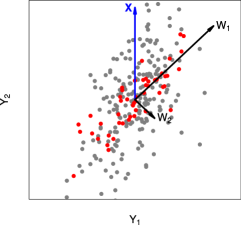
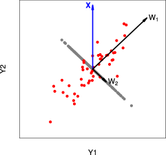
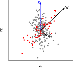
Figure 1: Naive RUV-2 (fixed $\alpha$) and random $\alpha$ based corrections, with $m=2$.

To summarize, given an estimate of $W$, we consider either a fixed or a random $\alpha$ model to estimate $X\beta$. For each of these we have either the naive option of estimating $\alpha$ for $X\beta=0$ or to minimize the joint likelihood of $(X\beta,\alpha)$ by iterating between the estimation of $X\beta$ and $\alpha$. The naive fixed $\alpha$ procedure corresponds to the naive RUV-2 of Gagnon-Bartsch and Speed (2012). We expect the other alternatives to lead to better estimates of $X\beta$.

3.3 Correlation on samples vs correlation on genes

In model (3) we arbitrarily chose to endow $\alpha$ with a distribution, which is equivalent to introducing an $m\times m$ covariance matrix $\Sigma$ on the rows of the $Y-X\beta$ residuals. If we choose instead to model the rows of $W$ as iid normal vectors with spherical covariance, we introduce a $n\times n$ covariance matrix $\Sigma^{\prime}$ on the columns of the $Y-X\beta$ residuals. In the supervised case and if we consider a random $\beta$ as well, the maximum a posteriori estimator of $\beta$ incorporates the prior encoded in $\Sigma^{\prime}$ by shrinking the $\beta_{j}$ of positively correlated genes towards the same value and enforcing a separation between the $\beta_{j}$ of negatively correlated genes. This approach was used in Desai and Storey (2012). As an example if $\alpha\in\mathbb{R}^{1\times n}$ is a constant vector, i.e., if $\Sigma^{\prime}$ is a constant matrix with an additional positive value on its diagonal, the maximum a posteriori estimator of $\beta$ boils down to the “multi-task learning” estimator (Evgeniou et al., 2005; Jacob et al., 2009) detailed in Appendix B. This model as is does not deal with any unwanted variation factor which may affect the samples. Using two noise terms in the regression model, one with correlation on the samples and the other one on the genes would lead to the same multi-task penalty shrinking some $\beta_{j}$ together, but with a $\|.\|^{2}_{\Sigma}$ loss instead of the regular Frobenius loss discussed in Appendix B.

Note that this discussion assumes $\Sigma^{\prime}$ is known and used to encode some prior on the residuals of the columns of $Y-X\beta$. If however $\Sigma^{\prime}$ needs to be estimated, and estimation is done using the empirical covariance of $Y-X\beta$, the estimators of $\beta$ derived from (3) and from the model with an $n\times n$ covariance $\Sigma^{\prime}$ on the $Y-X\beta$ residuals become very similar, the only difference being that in one case the estimator of $\alpha|W,Y-X\beta$ is shrinked and in the other case the estimator of $W|\alpha,Y-X\beta$ is shrinked.

4 Estimation of $W$

When $X$ is observed it is usual to introduce the classical mixed effect or generalized least square regression (Robinson, 1991; Freedman, 2005) for a fixed covariance $\Sigma$ first and to discuss the practical estimation in a second step. Similarly for each of the options discussed in Section 3, we rely on a particular estimate of $W$. A common approach coined feasible generalized least squares (FGLS) in the regression case (Freedman, 2005) is to start with an ordinary least squares step to estimate $\beta$ and then use some estimator of the covariance on $Y-X\beta$. Listgarten et al. (2010) used a similar approach to estimate their covariance matrix. An alternative is to use the restricted maximum likelihood (REML) estimator which corrects for the fact that the same data are used to estimate the mean $X\beta$ and the covariance, whereas the empirical covariance matrix maximizes the covariance assuming $X\beta$ is known. Listgarten et al. (2010) mention that they tried both ML and REML but that this did not make a difference in practice.

In this section, we discuss estimation procedures for $W$ which are relevant in the case where $X$ is not observed. As a general comment, recall that fixed $\alpha$ models such as naive RUV-2 require $\textrm{rank}(W)<\textrm{rank}(Y)$ otherwise the entire $Y$ is removed by the regression step, but random $\alpha$ models allow $\textrm{rank}(W)\geq\textrm{rank}(Y)$ because they lead to penalized regressions.

So far, we considered the estimate $\hat{W}_{2}$ used in supervised RUV-2, which relies on the SVD of the expression matrix restricted to its control genes. This estimate was shown to lead to good performance in supervised estimation (Gagnon-Bartsch and Speed, 2012). Unsupervised estimation of $X\beta$ may be more sensitive to the influence of the factor of interest $X$ on the control genes : in the case of fixed $\alpha$ models, if the estimated $W$ is very correlated with $X$ in the sense of the canonical correlation analysis (Hotelling, 1936), i.e., if there exists a linear combination of the columns of $X$ which has high correlation with a linear combination of the columns of $W$, then most of the association of the genes with $X$ will be lost by the correction. Random $\alpha$ models are expected to be less sensitive to the correlation of $W$ with $X$ but could be more sensitive to poor estimates of the variance carried by each direction of unwanted variation.

This suggests that unsupervised estimation methods could benefit from better estimates of $W$. We present two directions that could lead to such estimators.

4.1 Using replicates

We first consider “control samples” for which the factor of interest $X$ is $0$. In practice, one way of obtaining such control samples is to use replicate samples, i.e., samples that come from the same tissue but which were hybridized in two different settings, say across time or platform. The profile formed by the difference of two such replicates should therefore only be influenced by unwanted variation – those whose levels differ between the two replicates. In particular, the $X$ of this difference should be $0$. More generally when there are more than two replicates, one may take all pairwise differences or the differences between each replicate and the average of the other replicates. We will denote by $d$ the indices of these artificial control samples formed by differences of replicates, and we therefore have $X^{d}=0$ where $X^{d}$ are the rows of $X$ indexed by $d$.

4.1.1 Unsupervised estimation of $W\alpha$

A first intuition is that such samples could be used to identify $\alpha$ the same way Gagnon-Bartsch and Speed (2012) used control genes to estimate $W$. Therefore, we start by presenting how control samples can be used to estimate $W\alpha$ in an unsupervised fashion, and then discuss how the procedure yields a new estimator of $W$. We consider the following algorithm :

• Use the rows of $Y$ corresponding to control samples

  $$Y^{d}=W^{d}\alpha+\varepsilon^{d},$$ (10)

  to estimate $\alpha$. Assuming iid noise $\varepsilon_{j}\sim\mathcal{N}(0,\sigma^{2}_{\varepsilon}I_{m}),\,j=1,\ldots,n$, the $(W^{d}\alpha)$ matrix maximizing the likelihood of (10) is $\operatorname*{arg\,min}_{W^{d}\alpha,\textrm{rank}W^{d}\alpha\geq k}\|Y^{d}-W^{d}\alpha\|_{F}^{2}$. By the same argument used in Section 2 for the first step of RUV-2, this argmin is reached for $\hat{W^{d}\alpha}=PE_{k}Q^{\top}$, where $Y^{d}=PEQ^{\top}$ is the singular value decomposition (SVD) of $Y^{d}$ and $E_{k}$ is the diagonal matrix with the $k$ largest singular values as its $k$ first entries and $0$ on the rest of the diagonal. We can use $\hat{\alpha}=E_{k}Q^{\top}$.

• Plugging $\hat{\alpha}$ in (2), the maximum likelihood of $W$ is now solved by a linear regression, $\hat{W}=Y_{c}\hat{\alpha}^{\top}_{c}(\hat{\alpha}_{c}\hat{\alpha}_{c}^{\top})^{-1}$.

• Once $W$ and $\alpha$ are estimated, $\hat{W}\hat{\alpha}$ can be removed from $Y$.

$X$ is not required in this procedure which in itself constitutes an unsupervised correction for $Y$.

4.1.2 Comparison of the two estimators of $W$

This procedure also yields an estimator of $W$, which can be plugged in any of the procedures we discussed in Section 3. The estimator $\hat{W}_{2}$ we considered so far was obtained using the first left singular vectors of the control genes $Y_{c}$, which can also be thought of as a regression of the control genes on their first right singular vectors, i.e., the main variations $E_{k}Q^{\top}$ observed in the control genes. By contrast the estimator that we discuss here is obtained by a regression of the control genes against the main variations observed in the control genes for the control samples formed by differences of replicates. Assuming our control genes happen to be influenced by the factor of interest $X$, i.e., $\beta_{c}\neq 0$, the estimator of $W$ solely based on control genes may have more association with $X$ than it should, whereas the one using differences of replicate samples should not be affected. On the other hand, restricting ourselves to the variation observed in differences of replicates may be too restrictive because we don’t capture unwanted variation when no replicates are available.

To make things more precise, let us assume that the control genes are actually influenced by the factor of interest $X$ and that $\beta_{c}\sim\mathcal{N}(0,\sigma_{\beta_{c}}^{2})$. In this case we have $\mathbb{E}[Y_{c}Y_{c}^{\top}]=XX^{\top}\sigma_{\beta_{c}}^{2}+WW^{\top}\sigma_{\alpha}^{2}+I_{m}\sigma_{\varepsilon}^{2}$, so if we use $Y_{c}$ to estimate $W$ or $\Sigma$ as we do for $\hat{W}_{2}$ the estimate will be biased towards $X$. Let us now consider the estimator $\hat{W}_{r}$ obtained by the replicate based procedure. To simplify the analysis we assume that $k=d$ and therefore $\hat{\alpha}=Y^{d}$ in the procedure described in Section 4.1.1. Consequently $\hat{W}\hat{\alpha}=Y_{c}(Y_{c}^{d})^{\top}\left(Y_{c}^{d}(Y_{c}^{d})^{\top}\right)^{-1}Y^{d}$. Define $\hat{W}_{r}\stackrel{{\scriptstyle\Delta}}{{=}}Y_{c}(Y_{c}^{d})^{\top}\left(Y_{c}^{d}(Y_{c}^{d})^{\top}\right)^{-\frac{1}{2}}$. Assuming $X^{d}$ is indeed equal to $0$ we can develop :

$$\hat{W}_{r}=(X\beta_{c}+W\alpha_{c}+\varepsilon_{c})(W^{d}\alpha_{c}+\varepsilon_{c}^{d})^{\top}\left(W^{d}\alpha_{c}\alpha_{c}^{\top}(W^{d})^{\top}+W^{d}\alpha_{c}(\varepsilon_{c}^{d})^{\top}+\varepsilon_{c}^{d}\alpha_{c}^{\top}(W^{d})^{\top}+\varepsilon_{c}^{d}(\varepsilon_{c}^{d})^{\top}\right)^{-\frac{1}{2}}.$$

We now make some heuristic asymptotic approximations in order to get a sense of the behavior of $\hat{W}_{r}$. $\alpha_{c}\alpha_{c}^{\top}$ and $\varepsilon_{c}^{d}(\varepsilon_{c}^{d})^{\top}$ are Wishart variables which by the central limit theorem are close to $cI_{m}\sigma_{\alpha}^{2}$ and $cI_{m}\sigma_{\varepsilon}^{2}$ respectively if the number of control genes is large enough regardless how good the control genes are, i.e., how small $\sigma_{\beta_{c}}$ is. In addition dot products between independent multivariate normal variables are close to $0$ in high dimension so we approximate $\beta_{c}\alpha_{c}^{\top},\beta_{c}\varepsilon_{c}^{\top}$ and $\alpha_{c}\varepsilon_{c}^{\top}$ by $0$. The approximations involving $\beta_{c}$ depend in part how good the control genes are, but can still be valid for larger $\sigma_{\beta_{c}}$ if the number of control gene is large enough. We further assume that $\sigma_{\varepsilon}\ll\sigma_{\alpha}$ and that the control samples are independent from the samples for which we estimate $W$ and ignore the $cI_{m}\sigma_{\varepsilon}^{2}$ and $\varepsilon_{c}(\varepsilon_{c}^{d})^{\top}$ terms. Implementing all these approximations yields $\hat{W}_{r}\simeq\sigma_{\alpha}c^{\frac{1}{2}}W(W^{d})^{\top}\left(W^{d}(W^{d})^{\top}\right)^{\frac{1}{2}}$. Writing $W^{d}=A\Delta B^{\top}$ for the SVD of $W^{d}$, we obtain $\hat{W}_{r}\simeq\sigma_{\alpha}c^{\frac{1}{2}}WB_{r}A_{r}^{\top}$, where $r$ is the rank of $W^{d}$ and $A_{r},B_{r}$ contain the first $r$ columns of $A$ and $B$ respectively. This suggests that if $W^{d}$ has rank $k$ $\hat{W}_{r}$ is a good estimator of $W$ in the sense that it is not biased towards $X$ even if the control genes are influenced by $X$. If $W^{d}$ is column rank deficient, the $B_{r}$ mapping can delete or collapse unwanted variation factors in $\hat{W}_{r}$. The effect is easier to observe on the estimator of $\Sigma$ : $\hat{W}_{r}\hat{W}_{r}^{\top}\simeq\sigma^{2}_{\alpha}cWB_{r}B_{r}^{\top}W^{\top}$. Consider for example the following case with $3$ unwanted variation factors and $3$ replicate samples with unwanted variation $(1,0,3)$, $(0,1,3)$ and $(1,1,3)$. The $W^{d}$ and corresponding $B_{r}B_{r}^{\top}$ obtained by taking differences between replicates $(1,2)$, $(1,3)$ and $(3,2)$ are

$$W^{d}=\left(\begin{array}[]{c c c}1&-1&0\\ 0&-1&0\\ 1&0&0\end{array}\right)\qquad\textrm{ and }\qquad B_{r}B_{r}^{\top}=\left(\begin{array}[]{c c c}1&0&0\\ 0&1&0\\ 0&0&0\end{array}\right),$$

so the $B_{r}B_{r}^{\top}$ factor removes the third factor from the estimate of $\Sigma$. This is because the $3$ replicates have the same value for the third factor. Similarly if two factors are perfectly correlated on the replicate samples, e.g., the first two factors for $(1,1,0)$, $(0,0,1)$ and $(1,1,1)$, the $W^{d}$ and corresponding $B_{r}B_{r}^{\top}$ for the same differences between replicates $(1,2)$, $(1,3)$ and $(3,2)$ are

$$W^{d}=\left(\begin{array}[]{c c c}1&1&-1\\ 0&0&-1\\ 1&1&0\end{array}\right)\qquad\textrm{ and }\qquad B_{r}B_{r}^{\top}=\left(\begin{array}[]{c c c}1/2&1/2&0\\ 1/2&1/2&0\\ 0&0&1\end{array}\right),$$

which collapses the first two factors into an average factor and leaves the third one unchanged.

Finally, another option in the context of random $\alpha$ models is to combine the control gene based and replicate based estimators of $W$ by concatenating them. In terms of $\Sigma$, this amounts to summing the two estimators of the covariance matrix. This may help if, as in our first example, some factors are missing from $\hat{W}_{r}$ because all pairs of replicates have the same value for these factors. In this case, combining it with $\hat{W}_{2}$ could lead two an estimate containing less $X$ but still containing all the unwanted variation factors.

4.2 Using residuals

We already mentioned that in the case where $X$ is observed, a common way of estimating $W$ known as FGLS is to first do an ordinary regression of $Y$ against $X$, then compute the empirical covariance on the residuals $Y-X\hat{\beta}$. The estimators of $W$ that we discussed work around the estimation of $X\beta$ by using genes for which $\beta$ is known to be $0$ or samples for which $X$ is known to be $0$. Once we start estimating $X\beta$, e.g., by iterating over $X\beta$ and $\alpha$ as described at the end of Section 3 we can use a form of FGLS and re-estimate $W$ using $Y-\hat{X\beta}$. If the current estimator of $X\beta$ is correct, this amounts to making all the genes control genes, and all the samples control samples.

4.3 Using a known $W$

Finally in some cases we may want to consider that $W$ is observed. For example, if the dataset contains known technical batches, involves different platforms or labs, $W$ could encode these factors instead of being estimated from the data. In particular if the corresponding $W$ is a partition of the samples, then naively estimating $\alpha$ by regression using $X\beta=0$ and removing $W\hat{\alpha}$ from $Y$ corresponds to mean-centering the groups defined by $W$. In most cases however, this procedure or its shrunken equivalent doesn’t yield good estimates of $X\beta$. This was also observed by Gagnon-Bartsch and Speed (2012) in the supervised case. One reason is that this $W$ only accounts for known unwanted variation when other unobserved factors can influence the gene expression. The other one is that this approach leads to a linear correction for the unwanted variation in the representation used in $W$. If we know that gene expression is affected by the temperature of the scanner, setting a column of $W$ to be this temperature leads to a linear correction whereas the effect of the temperature may be quadratic, or involve interactions with other factors. In this case, estimating $W$ implicitly allows us to do a non-linear correction because the estimated $W$ could fit any non-linear representation of the observed unwanted variation which actually affects gene expression.

5 Result

We now evaluate our unsupervised unwanted variation correction methods on several microarray gene expression datasets. We focus on clustering, a common unsupervised analysis performed on gene expression data (Speed, 2003) typically to identify subtypes of a disease (Perou et al., 2000). Note that the proposed method is in no way restricted to clustering, which is simply used here to assess how well each correction did at removing unwanted variation without damaging the signal of interest.

Because of the unsupervised nature of the task, it is often difficult to determine whether the partition obtained by one method is better than the partition obtained by another method. We adopt the classical strategy of turning supervised problems into unsupervised ones : for each of the three datasets we consider in this section, a particular grouping of the samples is known and considered to be the factor of interest which must be recovered. Of course, the correction methods are not allowed to use this known grouping structure.

In order to quantify how close each clustering gets to the objective partition, we adopt the following squared distance (Bach and Harchaoui, 2007) between two given partitions $\mathcal{C}=(c_{1},...,c_{k})$ and $\mathcal{C}^{\prime}=(c^{\prime}_{1},...,c^{\prime}_{k})$ of the samples into $k$ clusters :

$$d(\mathcal{C},\mathcal{C}^{\prime})=k-\sum_{i,j=1}^{k}\frac{|c_{i}\cap c^{\prime}_{j}|^{2}}{|c_{i}||c^{\prime}_{j}|}.$$ (11)

This score ranges between $0$ when the two partitionings are equivalent, and $k-1$ when the two partitions are completely different. To give a visual impression of the effect of the corrections on the data, we also plot the data in the space spanned by the first two principal components, as PCA is known to be a convex relaxation of $k$-means (Zha et al., 2001). For each of the correction methods that we evaluate, we apply the correction method to the expression matrix $Y$ and then estimate the clustering using a $k$-means algorithm.

In addition to the methods we introduced in Sections 3 and 4 of this paper, we consider as baselines :

• An absence of correction,

• A centering of the data by level of the known unwanted variation factors.

• The naive RUV-2 procedure of Gagnon-Bartsch and Speed (2012).

Centering of the data by level of the known unwanted variation factors means that if several unwanted variation factors are expected to affect gene expression, we center each group of samples having the same value for all of the unwanted variation factors. Of course this implies that unwanted variation factors are known and this may not correct the effect of unobserved factors.

On each dataset, we evaluate three basic correction methods : the unsupervised replicate-based procedure described in Section 4.1.1, the random $\alpha$ model with $\hat{W}=\hat{W}_{2}$ and the random $\alpha$ model with $\hat{W}$ combining $\hat{W}_{2}$ and $\hat{W}_{r}$. For each of these three methods, we also evaluate an iterative version which alternates between estimating $\alpha$ using a ridge regression and estimating $X\beta$ using the sparse dictionary learning technique of (Mairal et al., 2010). The sparse dictionary estimator finds $(X,\beta)$ minimizing the objective :

$$\frac{1}{2}\|(Y-\widehat{W\alpha})-X\beta\|_{F}^{2}+\lambda\|\beta\|_{1},$$

under the constraint that $X\beta$ has rank $p$ and the columns of $X$ have norm $1$. The problem is not jointly convex in $(X,\beta)$ so there is no guarantee of obtaining a global minimizer. For the iterative methods, we also re-estimate $W$ using the $Y-\widehat{X\beta}$ residuals as discussed in Section 4.2 every $10$ iterations. Many other methods are possible such as iterative fixed $\alpha$ (for different estimators of $W$), random $\alpha$ using the $\hat{W}_{r}$ estimator introduced in Section 4.1.1 with or without iterations, with or without updating $W$, or replacing the sparse dictionary estimator by other matrix decomposition matrix techniques such as convex relaxations of $k$-means. We restrict ourselves to just the set of methods mentioned for the sake of clarity and because we think they illustrate the benefit of the different options that we discuss in this paper.

Some of the methods require the user to choose some hyper-parameters : the ranks $k$ of $W\alpha$ and $p$ of $X\beta$, the ridge $\nu$ and the strength $\lambda$ of the $\ell_{1}$ penalty on $\beta$. In order to decrease the risk of overfitting and to give good rules of thumb for application of these methods to new data, we tried to find relevant heuristics to fix these hyperparameters and to use them consistently on the three benchmarks. Some methods may have given better performances on some of these datasets for different choices of the hyperparameters. We discuss empirical robustness of the methods to their hyperparameters for each dataset. The rank $k$ of $W\alpha$ was chosen to be close to $m/4$, or to the number of replicate samples when the latter was smaller than the former. For methods using $p$, we chose $p=k$. For random $\alpha$ models, we use $k=m$ : the model is regularized by the ridge $\nu$. We do not combine it with a regularization of the rank. Since $\nu$ is a ridge parameter acting on the eigenvalues of $W^{\top}W$, we chose it to be $\sigma_{1}(W^{\top}W)\times 10^{-3}$, where $\sigma_{1}(A)$ is the largest eigenvalue of a positive semidefinite matrix $A$. Special care must be taken for the iterative methods : their naive counterparts use $X\beta=0$ and therefore minimize $\|Y-W\alpha\|_{F}^{2}$, whereas the iterative estimators minimize $\|Y-X\beta-W\alpha\|_{F}^{2}$ which can lead to corrections of smaller norm $\|W\alpha\|_{F}$. In order to make them comparable, we choose $\lambda$ such that $\|W\alpha\|_{F}$ is close to the one obtained with the non-iterative algorithm.

All experiments were done using R. For the experiments using sparse dictionary algorithms, we used the SPAMS software  developed by the first author of Mairal et al. (2010) under GPL license and for which an R interface is available.

5.1 Gender data

We first consider a 2004 dataset of patients with neuropsychiatric disorders. This dataset was published by Vawter et al. (2004) in the context of a gender study : the objective was to study differences in gene expression between male and female patients affected by these neuropsychiatric disorders. It was already used in Gagnon-Bartsch and Speed (2012) to study the performances of RUV-2 : the number of genes from the X and Y chromosomes which were found significantly expressed between male and female patients was used to assess how much each correction method helped. This gender study is an interesting benchmark for methods aiming at removing unwanted variation as it expected to be affected by several technical and biological factors : two microarray platforms, three different labs, three tissue localizations in the brain. Most of the $10$ patients involved in the study had samples taken from the anterior cingulate cortex (a), the dorsolateral prefontal cortex (d) and the cerebellar hemisphere (c). Most of these samples were sent to three independent labs : UC Irvine (I), UC Davis (D) and University of Michigan, Ann Arbor (M). Gene expression was measured using either HGU-95A or HGU-95Av2 Affymetrix arrays with $12,600$ shared between the two platforms. Six of the $10\times 3\times 3$ combinations were missing, leading to $84$ samples. We use as control genes the same $799$ housekeeping probesets which were used in Gagnon-Bartsch and Speed (2012). We use all possible differences between any two samples which are identical up to the brain region or the lab, leading to $106$ differences. Note that using all these replicates leads to non-iid data in the replicate based methods : each sample is dependent on all the differences in which it is involved. The discussion in Section 4.1.2 suggests that this could bias the estimation of $W$. However we seem to obtain reasonable results for this dataset. As a pre-processing, we also center the samples per array type.

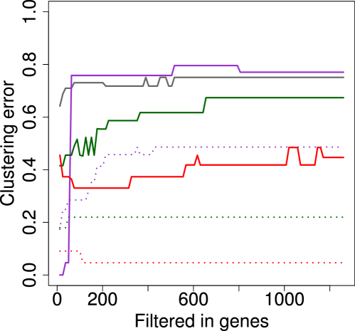
Figure 2: Clustering error against number of genes selected (based on variance) before clustering. Gray line : naive RUV-2, purple lines : replicate-based corrections, green lines : random $\alpha$ model using $\hat{W}_{2}$, red lines : random $\alpha$ model using a combination of $\hat{W}_{2}$ and $\hat{W}_{r}$. Full lines : no iteration, dotted lines : with iterations.

Since most genes are not affected by gender, and because $k$-means is known to be sensitive to noise in high dimension, clustering by gender gives better results in general when removing genes with low variance before applying $k$-means. For each of the methods assessed, we therefore try clustering after filtering different numbers of genes based on their variance on the corrected. Figure 2 shows the clustering error (11) for the methods against the number of genes retained. The uncorrected and mean-centering cases are not displayed to avoid cluttering the plot, but give values above $0.95$ for all numbers of genes retained. Figure 3 shows the samples in the space of the first two principal components in these two cases, keeping the $1260$ genes with highest variance. On the uncorrected data (left panel), it is clear that the samples first cluster by lab which is the main source of variance, then by brain region which is the second main source of variance. This explains why the clustering on uncorrected data is far away from a clustering by gender. Mean-centering samples by region-lab (right panel) removes all clustering per brain region or lab, but doesn’t make the samples cluster by gender. The gray line of Figure 2 shows the performance of naive RUV-2 for $k=20$. Since naive RUV-2 is a radical correction which removes all variance along some directions, it is expected to be more sensitive to the choice of $k$. The estimation is damaged by using $k=40$ (clustering error $0.99$). Using $k=5$ also degrades the performances, except when very few genes are kept.

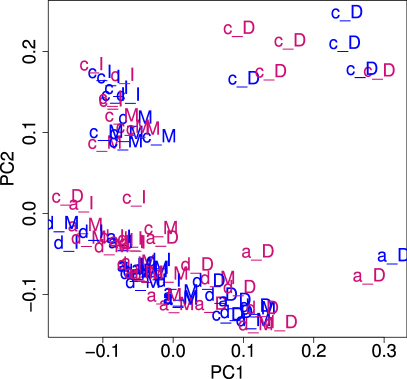
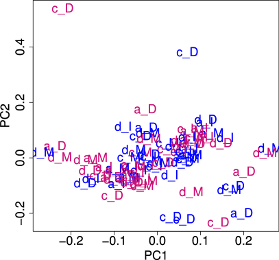
Figure 3: Samples of the gender study represented in the space of their first two principal components before correction (left panel) and after centering by lab plus brain region (right panel). Blue samples are males, pink samples are females. The labels indicate the laboratory and brain region of each sample. The capital letter is the laboratory, the lowercase one is the brain region.

The purple lines of Figure 2 represent the replicate-based corrections. The solid line shows the performances of the non-iterative method described in Section 4.1.1. Its performances are similar to the ones of naive RUV-2 in this case, except when very few genes are selected and the replicate-based method leads to a perfect clustering by gender. As for the naive RUV-2 correction, using a $k$ too large damages the performances. However, the replicate-based correction is more robust to overestimation of $k$ : using $k=40$ only leads to a $0.83$ error. This is also true for the other benchmarks, and can be explained by the fact that the correction is restricted to the variations observed among the contrasts of replicate samples which are less likely to contain signal of interest.

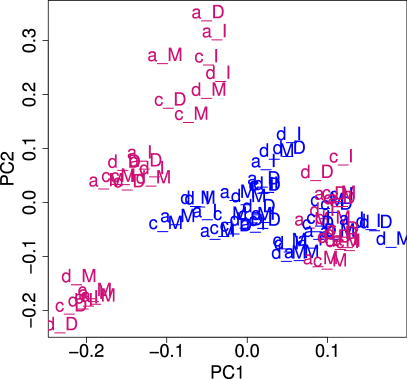
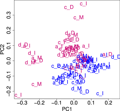
Figure 4: Using replicates. Left: no iteration, right: with iterations

The iterative version in dotted line leads to much better clustering except again when very few genes are selected. Figure 4 shows the samples in the space of the first two principal components after applying the non-iterative (left panel) and iterative (right panel) replicate-based method. The correction shrinks the replicates together, leading to a new variance structure, more driven by gender although not separating perfectly males and females. One may wonder whether this shrinking gives a better partition structure than clustering each region-lab separately, e.g. clustering only the samples taken from the cerebellar hemisphere and sent to UC Irvine. This actually leads to clustering errors higher than $0.89$ for all region-lab pairs, even when keeping only few genes based on their variance.

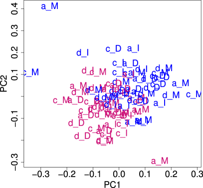
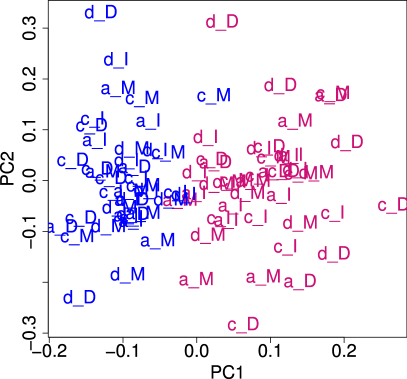
Figure 5: Random alpha with control genes only. Left: no iteration, right: with iterations

The green lines of Figure 2 correspond to the random $\alpha$ based corrections using the estimate of $W$ computed on control genes only. The solid line shows the results for the non-iterative method. Note that in this case, the $\nu=\sigma_{1}(W^{\top}W)\times 10^{-3}$ is not optimal, as larger $\nu$ lead to much lower clustering errors. This correction yields good results on this dataset, as illustrated by the reasonably good separation obtained in the space of the first two principal components after correction on the left panel of Figure 5. Note that the variance $\|W\alpha\|_{F}^{2}$ removed by the random $\alpha$ correction is larger that the one removed by naive RUV-2 and the replicate-based procedure. However the advantage of ridge RUV-2 does not come from its doing more deflation, it is rather a handicap here. As we discussed, random $\alpha$ with a larger penalty $\nu$, and therefore a smaller $\|W\alpha\|_{F}$, leads to better results. If we increase $k$ for the naive and replicate based procedures to get similar $\|W\alpha\|$ as the random $\alpha$ correction, we obtain clustering scores of $0.99$ and $0.83$ respectively.

In order for the random $\alpha$ correction to work, it is crucial to have a good estimate of $\Sigma$ or equivalently a good estimate $W$ with the information of how much variance is caused by unwanted variation along each direction. As a consequence, it is crucial in the unsupervised case, even more than in the supervised case, to have good control genes. This is probably why the random $\alpha$ based correction works well on gender data : few genes are actually influenced by gender so in particular the housekeeping genes contain little signal related to the factor of interest. The dotted green line of Figure 2 corresponds to the random $\alpha$ based corrections with iterations plus sparsity, which in this case leads to lower clustering errors. Here again, sparsity works well because lots of genes are not affected by gender. As a sanity check, we tried adding random genes to the control genes used in non-iterative methods but this did not lead to a clear improvement.

Finally, the red lines of Figure 2 correspond to the random $\alpha$ estimators using a combination $\hat{W}_{2}$ and $\hat{W}_{r}$. The full line corresponds to the non-iterative method, and shows that combining the two estimators of $W$ leads to a better correction than the two other methods which each rely on only one of these estimators. Recall however that the purple line uses $\hat{W}_{r}$ in a fixed $\alpha$ model, and therefore illustrates the improvement brought by using replicates to estimate $W$, compared to the gray line which only uses negative control genes. Using $\hat{W}_{r}$ with a random $\alpha$ model (not shown) leads to better performances than $\hat{W}_{2}$. Combining the estimators further improves the performances, although not by much. As for the previous methods, adding iterations to better estimate $\alpha$ improves the quality of the correction.

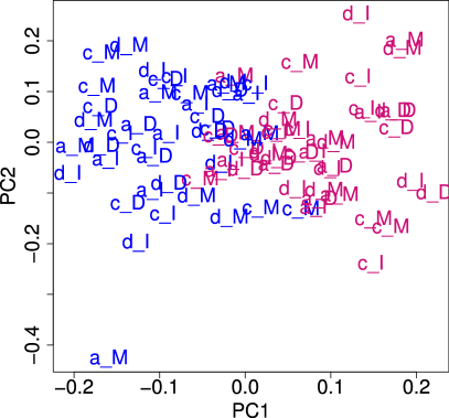
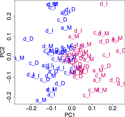
Figure 6: Random alpha with control genes only. Left: no iteration, right: with iterations

We also repeated the same experiment without centering the samples by array type. The performances were essentially the same as in the non-centered case for all methods, except that replicate based corrections do not work anymore and give clustering error $1$ for all numbers of filtered genes. This is expected since we don’t have replicates for array types and the replicate-based method has no way to correct for something which does not vary across the replicates. Using control genes however allows us to identify and remove the array type effect.

5.2 TCGA glioblastoma data

5.2.1 Data

We now illustrate the performances of our method on the gene expression array data generated in the TCGA project for glioblastoma (GBM) tumors (Cancer Genome Atlas Research Network, 2008). These tumors were studied in detail in Verhaak et al. (2010). For each of the $460$ samples, gene expression was measured on three different platforms : Affymetrix HT-HG-U133A Genechips at the Broad Institute, Affymetrix Human Exon 1.0 ST Genechips at Lawrence Berkeley Laboratory and Agilent 244K arrays at University of North Carolina. Verhaak et al. (2010) selected $200$ tumors and $2$ normal samples from the dataset based on sample quality criterions and filtered $1740$ genes based on their coherence among the three platforms and their variability within each platform. The expression values from the three platforms were then merged using factor analysis. They identified four GBM subtypes by clustering analysis on this restricted dataset : Classical, Mesenchymal, Proneural and Neural. We study these $202$ samples across the three platforms, keeping all the $11861$ genes in common across the three platforms. Among these $202$ samples, $173$ were identified by Verhaak et al. (2010) as “core” samples : they were good representers of each subtypes. $38$ of them are Classical, $56$ Mesenchymal, $53$ Proneural and $26$ Neural.

5.2.2 Design

For the purpose of the experiment, we study how well a particular correction allows us to recover the correct label of the $147$ Classical, Mesenchymal and Proneural tumors, leaving the other ones aside. Our objective is to recover the correct subtypes using a $k$-means with $3$ clusters. We consider two settings. In the first one, we use a full design with all $147$ samples from $3$ platforms. In the second one we build a confounding setting in which we only keep the Classical samples on Affymetrix HT-HG-U133A arrays, the Mesenchymal samples on Affymetrix Human Exon arrays and the Proneural samples on Agilent 244K arrays. In each case, we use $5$ randomly selected samples that we keep for all $3$ platforms and use as replicates. We do not use other samples as replicates even in the full design when all samples could potentially be used as replicates. Among the $5$ selected samples one was Neural, two Proneural, and two were not assigned a subtype. The results presented are qualitatively robust to the choice of these replicates.

In the confounded design, a correction which simply removes the platform effect is likely to also lose all the subtype signal because it is completely confounded with the platform, up to the replicate samples. The reason why we only keep $3$ subtypes is to allow such a total confounding of the subtypes with the $3$ platforms. However in this design, applying no correction at all is likely to yield a good clustering by subtype because we expect the platform signal to be very strong. A good correction method should therefore perform well in both the confounded and the full design. In the full design, the platform effect is orthogonal to the subtype effect so we expect the correction to be easier. Of course in this case, the uncorrected data is expected to cluster by platform which this time is very different from the clustering by subtype since each sample is present on each platform.

5.2.3 Result

Method	Full	Confounding
No correction	$2$	$0$
Mean-centering	$0.3$	$1.93$
Ratio method	$0.31$	$0.79$
Naive RUV-2	$2$	$0$
Random $\alpha$	$0.21$	$1.5$
+ iterations	$0.15$	$1$
Replicate based	$0.2$	$0.61$
+ iterations	$0.17$	$0.16$
Combined	$1.3$	$1.2$
+ iterations	$1.3$	$1$

Table 1: Clustering error of TCGA GBM data with full and confounded designs for various correction methods. Since there are $3$ clusters, errors range between $0$ and $2$.

Table 1 shows the clustering error obtained for each correction method on the two designs. Recall that since there are $3$ clusters, clustering errors range between $0$ and $2$. Most of the plots of the corrected data in the space spanned by the first two principal components are deferred to appendix C. As expected, the uncorrected data give a maximal error on the full design and $0$ in the presence of confounding. This is because, as seen on Figure 7, the uncorrected data cluster by platform which in the full design are orthogonal to the subtypes and in the second design are confounded with subtypes. For similar reasons, centering the data by platform works well in the full design but fails when there is confounding because removing the platform effect removes most of the subtype effect. When replicates are available, a variant of mean centering is to remove the average of replicate samples from each platform. This is known as the ratio method (Luo et al., 2010) and does improve on regular mean-centering in the presence of confounding. A disadvantage of this method is that it amounts to considering that $W$ is a partition of the data by batch (in this case by platform) whereas as discussed in Section 4.3 the actual unwanted variation may be a non linear function of the batch, possibly involving other factors. Note that we do not explicitly assess the ratio method for the other benchmarks because all samples are used as replicates so the ratio methods becomes equivalent to mean centering.

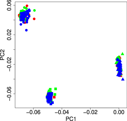
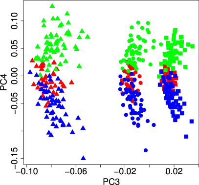
Figure 7: Uncorrected full design GBM data in the space of their first four principal components. Left panel : PC 1 and 2, right panel : PC 3 and 4. Colors denote subtypes, shapes denote platforms.

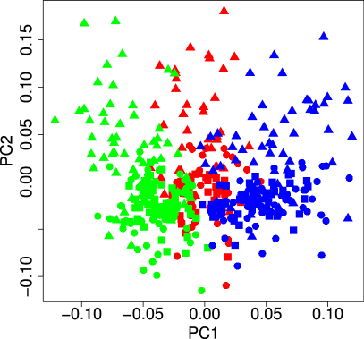
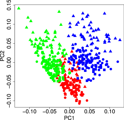
Figure 14: GBM full design random $\alpha$ with and without iterations. Colors represent subtypes, shapes represent platforms.

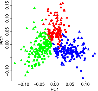
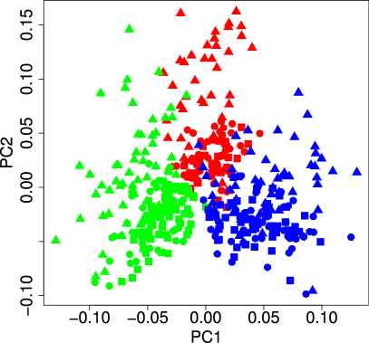
Figure 15: GBM full design replicate-based with and without iterations. Colors represent subtypes, shapes represent platforms.

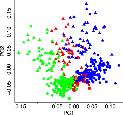
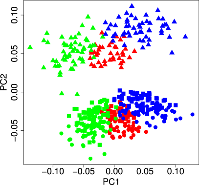
Figure 16: GBM full design combined with and without iterations. Colors represent subtypes, shapes represent platforms.

Naive RUV-2 gives a maximal error in the full design, $0$ otherwise. This result is actually caused by the fact that naive RUV-2 is extremely sensitive to the choice of $k$. Since the total number of differences formed on the $15$ replicates is $10$, we use $k=2$ as a default for naive RUV-2 and the replicate based procedure. In the full design, the platform effect is contained in the first three principal components of the control gene matrix $Y_{c}$ and the fourth principal component contains the subtype effect. This can clearly be seen on Figure 7. Removing only one or two directions of variance leaves too much platform effect. Removing a third one ($k=3$) gives a small error of $0.15$ and removing a fourth one gives an error of $1.83$. When the platform is confounded with the subtype, removing one or two components leads to a perfect clustering by subtype because the third principal component still contains platform/subtype signal. Removing more does not allow us to recover a clustering by subtype. So if we used $k=3$ instead of $k=2$, the result would be inverted : good for the full design, bad in the presence of confounding. The random $\alpha$ model works well in the full design, less so in the presence of confounding, as illustrated on Figure 14 and 17 respectively. While it was reasonably robust to the choice of the ridge parameter $\nu$ on the gender data, it is more sensitive on this one. Using $\nu=\sigma_{1}(W^{\top}W)\times 5.10^{-2}$ instead of $10^{-3}$ does not remove enough platform effect and leads to an error of $2$ on the full design, $0$ in the presence of confounding. Using a smaller factor of $5.10^{-4}$ leads to an error of $0.27$ ($1.65$ with confounding), and $10^{-4}$ to an error of $1.94$ ($1.98$ with confounding). Because the correction made by the random $\alpha$ model is softer than the one of the fixed $\alpha$ naive RUV-2, using $\nu=\sigma_{1}(W^{\top}W)\times 10^{-3}$ allows us to recover subtype signal in both designs. The sensitivity to $\nu$ is likely to be caused by the large difference of magnitude between $\sigma_{1}(W^{\top}W)$ and the next eigen values : the first one represents $98\%$ of the total variance. This is to be expected in most cases in presence of a strong technical batch effect. In both designs, using iterating between estimation of $X\beta$ using sparse dictionary learning and estimation of $\alpha$ using ridge regression further improves the performances. The replicate-based correction gives good results for both designs, as illustrated on Figure 15 and 18. Like for the gender data, it seems to be robust to the choice of $k$. For $k=10$ it gives errors $0.2$ and $0.53$ in the first and second design respectively. Here again, adding iterations on $(X\beta,\alpha)$ improves the quality of the correction in each case. Finally the combined method gives a clustering error of $1.3$ and $1.2$ in the first and second design respectively. This is not a very good performance but the method still manages to retain some of the factor of interest and does so consistently in the presence and in the absence of confounding. The corresponding corrected data are shown in Figure 16 and 19 for the full and confounded design respectively. Iterations improve the performance in the confounding design and do not change the result in the full design. Figure 16 suggests that for the full design, the problem comes from the fact that the correction does not remove all of the platform effect.

Note that, as with the gender data, the difference observed between the correction methods cannot be only explained by the fact that some of them remove more variance than others. For example in the full design, naive RUV-2, the replicate based procedure and the random $\alpha$ correction lead to similar $\|W\alpha\|_{F}$ but to very different performances : naive RUV-2 fails to remove enough platform signal whereas the other corrections remove enough of it for the arrays to cluster by subtype. In the confounding design, both naive RUV-2 and the replicate based procedure lead to similar $\|W\alpha\|_{F}$ and similar performances. The random $\alpha$ correction leads to a larger $\|W\alpha\|_{F}$ which explains its poor behavior. Estimating what amount of variance should be removed is part of the problem, so it would not be correct to conclude that the random $\alpha$ correction works as well as the others in this case. It is however interesting to check whether the problem of a particular method is its removing too much or not enough variance or whether it is a qualitative problem.

5.3 MAQC-II data

We finally assess our correction methods on a gene expression dataset which was generated in the context of the MAQC-II project (Shi et al., 2010). The study was done on rats and the objective was to assess hepatotoxicity of $8$ drugs. For each drug, three time points were done for three different doses. For each of these $8\times 3\times 3$ combinations, $4$ animals were tested for a total of $288$ animals. For each animal, one blood and one liver sample were taken. Gene expression in blood and in the liver were measured using Agilent arrays and gene expression in the liver was also measured using Affymetrix arrays. The Agilent arrays were loaded using the marray R package. Each array was loess normalized, dye swaps were averaged and each gene was then assigned the median log ratio of all probesets corresponding to the gene. The Affymetrix arrays were normalized using the gcrma R package. Each gene was then assigned the median log ratio of all probesets corresponding to the gene. For this experiment we retain samples from all platforms and tissues for the highest dose of each drug and for the last two time points $24$ hours and $48$ hours. Most of these drugs are not supposed to be effective for the earlier time points. This leads to a set of $186$ arrays that we restrict to the $9502$ genes which are common to all platforms. Each sample has a replicate for each tissue and platform, but there is no replicate against the time effect. For control genes, we used the same list of housekeeping genes as for the other datasets but converted to their rat orthologs, leading to $210$ control genes.

The interest of this complex design is obvious for the purpose of this paper : the resulting dataset contains a large number of arrays measuring gene expression influenced by the administered drug which we consider to be our factor of interest and by numerous unwanted variation factors. Array type, tissue, time and dose are likely to influence gene expression, preventing the arrays from clustering by drug. This clustering problem is much harder than the gender and glioblastoma ones. First of all, the drug signal may not be as strong as the gender which at least for a few genes is expected to be very clear or as the glioblastoma subtypes which were defined on the same dataset. Second and maybe more important, it is an $8$-class clustering problem, which is intrinsically harder than $2$- or $3$-class clusterings. Finally as we discuss in Section 5.4, the control genes for this dataset do not behave as expected.

Method	Error
No correction	$5.9$
Mean-centering	$5.1$
Naive RUV-2	$6.6$
Random $\alpha$	$4.7$
+ iteration	$5.4$
Replicate based	$2.8$ – $3.8$
+ iterations	$2.8$ – $3.8$
Combined	$5.7$
+ iterations	$5.7$

Table 2: Clustering error of MAQC-II data for various correction methods.

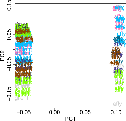
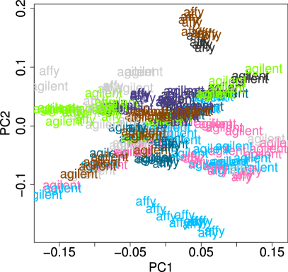
Figure 8: Samples of the MAQC-II study represented in the space of their first two principal components before correction (left panel) and after centering by tissue and platform region (right panel). Each color represents a different drug. The labels indicate the platform of each sample.

The errors obtained after applying each correction are displayed in Table 2. Recall that for this dataset, we are trying to recover a partition in $8$ classes corresponding to the $8$ drugs of the study so the maximum clustering error is $7$. The left panel of Figure 8 represents the uncorrected samples in the space of the first two principal components. The first principal components is clearly driven by the presence of two different types of arrays. The clustering error in this case is $5.9$. Centering by platform-tissue, i.e. centering separately the Affymetrix arrays, the Agilent liver and the Agilent blood, the data points do not cluster by platform anymore but just like for the gender data this does not lead to a clear clustering by drug. This can be seen on the right panel of Figure 8. The resulting clustering error is $5.1$. The naive RUV-2 correction doesn’t lead to any improvement compared to the uncorrected data, leading to an error of $6.6$. The random $\alpha$ estimator hardly improves the performances, and its iterative variant even increases a little the error. Figure 9 shows that these methods lead to a better organization of the samples by drug, but still far from a clean clustering. The replicate-based method leads to better performances. Even though we do $200$ runs of $k$-means to minimize the within sum of square objective, different occurrences of the $200$ runs lead to different clusterings with close objectives. We choose to indicate the range of clustering errors given by these different clusterings ($2.8$–$3.8$). The iterative version of the estimator gives the same range of errors. Figure 10 shows that these corrections indeed lead to a better organization of the samples by drugs in the space spanned by the first two principal components, but fails to correct the time effect against which no replicate is available. Finally the combined method gives poor performances. Figure 11 shows that it does not correct enough and that the data still cluster by platform. Increasing the magnitude of the correction by using a smaller ridge $\nu$ removes the platform effect but still doesn’t lead to a good clustering by drug. As it can be seen on Figure 11, the iterative version of the estimator leads to a very similar and equally poor estimate. The deflation $\|W\alpha\|_{F}$ obtained by the naive RUV-2 and replicate based procedures are larger than the one obtained by the random $\alpha$ correction, but this is not the reason for the replicate based procedure to work better than the random $\alpha$ correction : the former is quite robust to changes in $k$ and the latter does not improve when changing $\nu$.

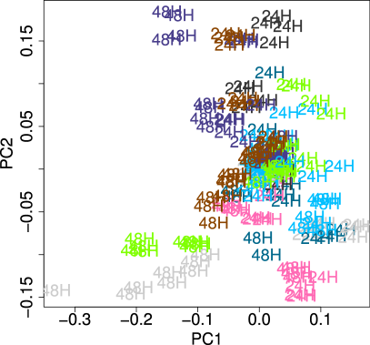
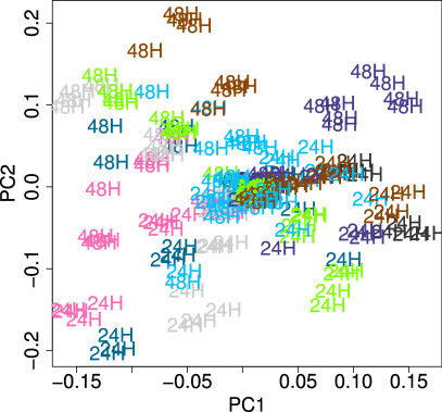
Figure 9: Samples of the MAQC-II study represented in the space of their first two principal components after applying the random $\alpha$ correction (left panel) and its iterative variant (right panel). Each color represents a different drug. The labels indicate the time of each sample.

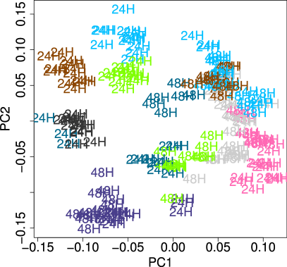
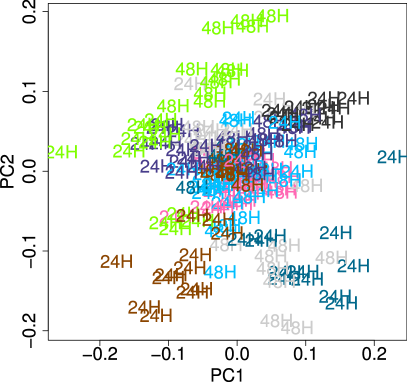
Figure 10: Samples of the MAQC-II study represented in the space of their first two principal components after applying the replicate-based correction (left panel) and its iterative variant (right panel). Each color represents a different drug. The labels indicate the time of each sample.

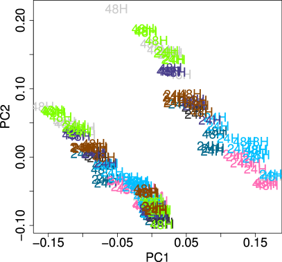
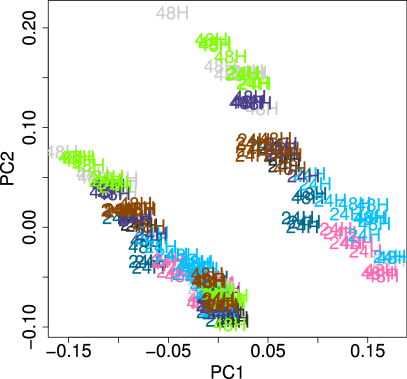
Figure 11: Samples of the MAQC-II study represented in the space of their first two principal components after applying the combined correction (left panel) and its iterative variant (right panel). Each color represents a different drug. The labels indicate the time of each sample.

5.4 Benefit of control genes

We have assumed so far that control genes had little association with $X$ and allowed proper estimation for the methods we introduced. In this section, we assess this hypothesis on our three benchmarks. Table 3 reproduces the results on the first two benchmarks of the non-iterative methods that we considered and which make use of control genes. In addition for each method and each of our first two benchmarks, we show the performance of the same method using all genes as control genes. For the gender data, we give the clustering error when filtering in $1260$ genes, which correspond to the last point of Figure 2.

Method	Gender control	Gender all genes	GBM 1 control	GBM 1 all genes	GBM 2 control	GBM 2 all genes
Naive RUV-2	$0.75$	$0.92$	$2$	$1.52$	$0$	$0.93$
Replicate-based	$0.77$	$0.77$	$0.2$	$0.25$	$0.61$	$0.37$
Random $\alpha$	$0.67$	$0.99$	$0.21$	$0.24$	$1.5$	$1.8$
Combined	$0.45$	$0.54$	$1.3$	$1.3$	$1.2$	$1.8$

Table 3: Clustering error of gender and glioblastoma data with full (1) or confounded (2) designs for various correction methods relying on control genes using either all genes or control genes.

The results of MAQC-II data are not presented in Table 3 but the result of each method is the same whether we use our control genes or all the genes for this dataset. Overall, we can see that some methods are affected by the use of control genes on the gender data, but using all the genes only mildly affects the performances of most methods on the GBM dataset, and as we said do not affect the performances on the MAQC-II dataset at all. This suggests that the genes that we used as control genes were indeed less affected by the factor of interest for the gender data but were not for the glioblastoma and MAQC-II data. This is consistent with the fact that methods which rely heavily on the control genes like naive RUV-2 and random $\alpha$ are very sensitive to the amplitude of the correction for the glioblastoma dataset and do not work for the MAQC-II dataset. As one may expect from the discussion of Section 4.1.2, methods using replicates, i.e., the replicate-based one introduced in Section 4.1.1 and the combined one seem less affected than methods that solely rely on control genes, even on the gender dataset. Remember that our replicate-based procedure estimates $W$ by regressing the control genes $Y_{c}$ against the variations observed among constrasts of replicates which can make it robust to the fact that control genes are affected by the factor of interest.

In order to verify the fact that the control genes used for the gender data are good control genes whereas the ones used for the other datasets are not good control genes, we show the CCA of all control genes and all non-control genes with the factor of interest $X$ as a boxplot for each dataset on Figure 12. Interestingly, the control genes used in the gender data are typically more associated with $X$ than the non-control genes whereas the opposite is observed for the glioblastoma and MAQC-II datasets. This seems to contradict the fact that control genes help identifying $W$ in the gender data and does not in the two others. Since $W$ is essentially estimated using PCA on $Y_{c}$ which is a multivariate procedure, we represent the first canonical correlation of $X$ with the eigen space corresponding to the $k$ first eigenvectors as a function of $k$ on Figure 13. It is clear from the figure that for the gender dataset the eigen space built using control genes has a smaller association with $X$ than the one built using non-control genes whereas this is much less clear for the two other datasets.

Figure 12: boxplot of the CCA of control and non-control genes with the factor of interest $X$ for the gender (left panel), glioblastoma (center panel) and MAQC-II (right panel) datasets.

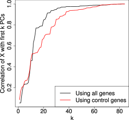
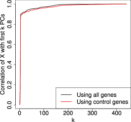
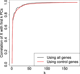
Figure 13: First canonical correlation of the factor of interest $X$ with the space spanned by the $k$ first eigenvectors of the empirical covariance computed on control genes (in red) and non-control genes (in black) against $k$ for the gender (left panel), glioblastoma (center panel) and MAQC-II (right panel) datasets.

To conclude, the case of gender data suggests that when good control genes are available they do help estimate and remove unwanted variation, especially for estimators which do not use replicate samples. The notion of good control samples seems to have more to do with the fact that the directions of maximum variance among these genes are not associated with $X$ than with individual univariate association of the genes with $X$. When control genes are as associated as the other genes with $X$, methods using replicate samples still give reasonable estimates and other methods become either ineffective or very sensitive to the amplitude of the correction.

6 Discussion

We proposed methods to estimate and remove unobserved unwanted variation from gene expression data when the factor of interest is also unobserved. In particular, this allows us to recover biological signal by clustering on datasets which are affected by various types of batch effects. The methods we introduced generalized the ideas of Gagnon-Bartsch and Speed (2012) and used two types of controls : negative control genes, which are assumed not to be affected by the factor of interest and can therefore be used to estimate the structure of unwanted variation, and replicate samples, whose differences are by construction not affected by the factor of interest. Differences of replicate samples can therefore also be used to estimate unwanted variation.

On three gene expression benchmarks, we verified that when good negative control genes were available, the correction techniques that used these negative controls were able to successfully estimate and remove unwanted variation, leading to the expected clustering of the samples according to the factor of interest. When the negative control genes are affected by the factor of interest, these techniques become less efficient, but replicate-based methods are successful at removing unwanted variation with respect to which replicates are available. Correcting for unwanted variation with respect to which replicates are given may sound less useful, because it implies that the unwanted variation is an observed factor such as a batch or a platform. However, even in this case, our techniques which estimate the unwanted variation factor outperform methods which use the known factor. This can be explained by the fact that the actual factor affecting the samples may be a non-linear function of the observed factor. In addition, replicates with respect to an observed unwanted variation factor may embed unknown unwanted variation. This suggests that when both types of controls are available, replicate based correction is a safer option, as it removes some unwanted variation and in the worst case scenario leaves some other unwanted variation in the data. Negative control gene based methods can remove more unwanted variation but run the risk to remove some signal of interest if the control genes were actually affected by the factor of interest. While the quality of negative control genes did affect the relative ranking of the two families of techniques, both gave reasonable performances on the first two benchmarks, indicating that they could be helpful on real data for this difficult estimation problem.

For both families of methods, we also proposed iterative versions of the techniques, which alternate between solving an unsupervised estimation problem for a fixed estimate of the unwanted variation, and estimating unwanted variation using the current estimate of the signal of interest. This approach often improved the latter estimate and never damaged the performances.

When the objective is to do clustering, the correction may benefit from more appropriate surrogates than the sparse dictionary learning problem. Better techniques to choose the hyperparameter $\nu$ for the random $\alpha$ based methods could also improve the performances.

Appendix A Proof of Proposition $1$

The left hand side of (8) is a standard ridge regression and has a closed form solution :

$$\alpha^{*}\stackrel{{\scriptstyle\Delta}}{{=}}\operatorname*{arg\,min}_{\alpha\in\mathbb{R}^{k\times n}}\left\{\|R-W\alpha\|^{2}_{F}+\nu\|\alpha\|^{2}_{F}\right\}=\left(W^{\top}W+\nu I_{k}\right)^{-1}W^{\top}R,$$

so for any $R\in\mathbb{R}^{k\times n}$,

$$\min_{\alpha\in\mathbb{R}^{k\times n}}\left\{\|R-W\alpha\|^{2}_{F}+\nu\|\alpha\|^{2}_{F}\right\}=\left\|\left(I_{m}-W\left(W^{\top}W+\nu I_{k}\right)^{-1}W^{\top}\right)R\right\|^{2}_{F}$$

$$+\nu\left\|\left(W^{\top}W+\nu I_{k}\right)^{-1}W^{\top}R\right\|^{2}_{F}$$

$$= \textrm{\bf tr }R^{\top}\biggl{(}I_{m}-2W\left(W^{\top}W+\nu I_{k}\right)^{-1}W^{\top}+W\left(W^{\top}W+\nu I_{k}\right)^{-1}W^{\top}W\left(W^{\top}W+\nu I_{k}\right)^{-1}W^{\top}$$

$$+\nu W\left(W^{\top}W+\nu I_{k}\right)^{-2}W^{\top}\biggr{)}R,$$

where we used the fact that $\|A\|_{F}^{2}=\textrm{\bf tr }A^{\top}A$. This is $\textrm{\bf tr }R^{\top}\left(I_{m}+WBW^{\top}\right)R$ with :

$$B \stackrel{{\scriptstyle\Delta}}{{=}}\left(W^{\top}W+\nu I_{k}\right)^{-1}W^{\top}W\left(W^{\top}W+\nu I_{k}\right)^{-1}+\nu\left(W^{\top}W+\nu I_{k}\right)^{-2}-2\left(W^{\top}W+\nu I_{k}\right)^{-1}$$

$$=\left(W^{\top}W+\nu I_{k}\right)^{-1}\left(W^{\top}W\left(W^{\top}W+\nu I_{k}\right)^{-1}+\nu\left(W^{\top}W+\nu I_{k}\right)^{-1}-2I_{k}\right)$$

$$=\left(W^{\top}W+\nu I_{k}\right)^{-1}\left(\left(W^{\top}W+\nu I_{k}\right)\left(W^{\top}W+\nu I_{k}\right)^{-1}-2I_{k}\right)$$

$$=-\left(W^{\top}W+\nu I_{k}\right)^{-1},$$

so

$$\min_{\alpha\in\mathbb{R}^{k\times n}}\left\{\|R-W\alpha\|^{2}_{F}+\nu\|\alpha\|^{2}_{F}\right\} =\textrm{\bf tr }R^{\top}\left(I_{m}-W\left(W^{\top}W+\nu I_{k}\right)^{-1}W^{\top}\right)R$$

$$=\|R\|^{2}_{S(W,\nu)}.$$

Appendix B Estimator of $\beta$ for a particular $\Sigma^{\prime}$ defined on the columns of the residuals

We consider the following model :

$$Y=X\beta+\tilde{\varepsilon},$$ (12)

where $Y,\tilde{\varepsilon}\in\mathbb{R}^{m\times n}$, $X\in\mathbb{R}^{m\times p}$, $\beta\in\mathbb{R}^{p\times n}$. We further assume that each row of $\tilde{\varepsilon}$ is distributed as $\mathcal{N}(0,\Sigma^{\prime})$ where $\Sigma^{\prime}\in\mathbb{R}^{n\times n}$ is a covariance matrix. Note that this is different from (3) where the $m\times m$ covariance was defined on the rows of $\tilde{\varepsilon}$.

(12) is equivalent to

$$Y=X\beta+W\alpha+\varepsilon,$$ (13)

where each column $W_{j}$ of $W$ is such that $W_{j}\stackrel{{\scriptstyle iid}}{{\sim}}\mathcal{N}(0,\sigma_{W}^{2}I_{m})$, $\varepsilon_{ij}\stackrel{{\scriptstyle iid}}{{\sim}}\mathcal{N}(0,\sigma^{2})$ and $\alpha\in\mathbb{R}^{k\times n}$ for some $k\leq m$ is such that $\alpha^{\top}\alpha+\sigma^{2}I_{m}=\Sigma^{\prime}$.

Assume $k=1$ and $\alpha=\mathbf{1}^{\top}$, where $\mathbf{1}$ is the all-one vector in $\mathbb{R}^{n}$. Then $\Sigma^{\prime}=\sigma^{2}I_{n}+\mathbf{1}\mathbf{1}^{\top}$, i.e. a constant matrix plus some additional constant on the diagonal. In this special case, $W$ is a single standard normal column vector and (13) can be written :

$$Y =X\beta+W\alpha+\varepsilon$$

$$=X\beta+W\mathbf{1}^{\top}+\varepsilon$$

$$=X\left(\beta+(X^{\top}X)^{-1}X^{\top}W\mathbf{1}^{\top}\right)+\varepsilon+R,$$

where $R$ is the projection of $W\mathbf{1}^{\top}$ to the orthogonal space of $X$. We can disregard it because a noise orthogonal to $X$ has no effect on a regression against $X$. Denoting $V\stackrel{{\scriptstyle\Delta}}{{=}}(X^{\top}X)^{-1}X^{\top}W\mathbf{1}^{\top}$, we see that (12) with this particular covariance is equivalent to assuming $Y=Xb+\varepsilon$, where $b=\beta+V$. Each column of $V$ is equal to $v=(X^{\top}X)^{-1}X^{\top}W$, i.e., to the projection of $W$ on $X$. If $\beta$ is assumed to be non-random and we estimate it by maximum likelihood we recover the regular OLS : $\beta+V$ is not identifiable. If we add a normal prior on $\beta$, the MAP equation is :

$$\max_{\beta,v}L(\beta,v|X,Y) \propto\max_{\beta,v}L(X,Y|\beta,v)p(\beta)p(v)$$ (14)

$$=\max_{\beta,v}\left\{\log L(X,Y|\beta,v)+\log p(\beta)+\log p(v)\right\}$$ (15)

$$=\min_{\beta,v}\|Y-X(\beta+V)\|_{F}^{2}+\lambda\|\beta\|^{2}_{F}+\nu\|v\|^{2}_{F},$$ (16)

where $\lambda,\nu$ depend on the prior variances of $\beta$ and $\alpha$. Then plugging $b=\beta+V$ and denoting its columns by $b_{i}$,

$$\min_{\beta,v}\left\{\|Y-X(\beta+V)\|_{F}^{2}+\lambda\|\beta\|^{2}_{F}+\nu\|v\|^{2}_{F}\right\}$$

$$=\min_{b,v}\left\{\|Y-Xb\|_{F}^{2}+\lambda\sum_{i=1}^{n}\|b_{i}-v\|^{2}_{F}+\nu\|v\|^{2}_{F}\right\}$$

$$=\min_{b}\left\{\|Y-Xb\|_{F}^{2}+\lambda\min_{v}\left(\sum_{i=1}^{n}\|b_{i}-v\|^{2}_{F}+\frac{\nu}{\lambda}\|v\|^{2}_{F}\right)\right\}$$

$$=\min_{b}\left\{\|Y-Xb\|_{F}^{2}+\lambda\sum_{i=1}^{n}\|b_{i}-\bar{b}\|^{2}_{F}+\nu\|\bar{b}\|^{2}_{F}\right\},$$

where $\bar{b}\stackrel{{\scriptstyle\Delta}}{{=}}\operatorname*{arg\,min}_{v}\left(\sum_{i=1}^{n}\|b_{i}-v\|^{2}_{F}+\frac{\nu}{\lambda}\|v\|^{2}_{F}\right)$ is a shrinked average of the $b_{i}$. The first equality is replacing $\beta+V$ by $b$ and $\beta$ by $b-V$. The second equality is moving the $\min_{v}$ to the part which depends on $v$. The last equality carries out the minimization over $v$.

Adding a block structure to $\Sigma^{\prime}$, or equivalently rows to $\alpha$ which are $1$ for some genes and $0$ for others, leads to an additional regularizer which penalizes the sum of squares among the $\beta_{i}$ within each block.

Appendix C PCA plots for the GBM data

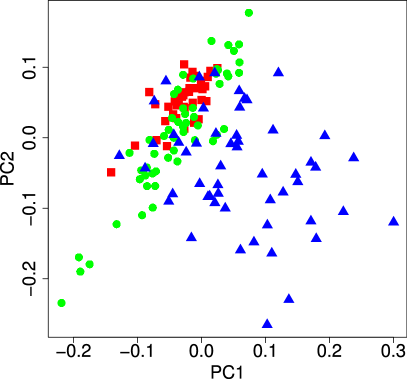
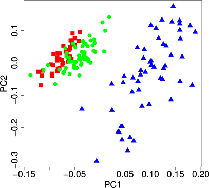
Figure 17: GBM confounded design random $\alpha$ with and without iterations. Colors represent subtypes, shapes represent platforms.

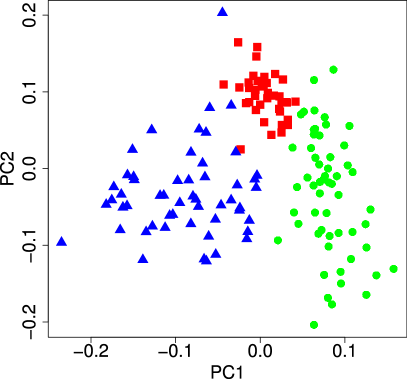
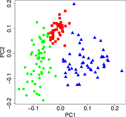
Figure 18: GBM confounded design replicate-based with and without iterations. Colors represent subtypes, shapes represent platforms.

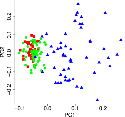
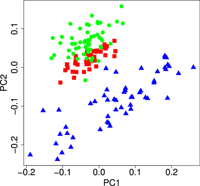
Figure 19: GBM confounded design combined with and without iterations. Colors represent subtypes, shapes represent platforms.

References

- Alter et al. (2000) O. Alter, P. O. Brown, and D. Botstein. Singular value decomposition for genome-wide expression data processing and modeling. Proc Natl Acad Sci U S A, 97(18):10101–10106, Aug 2000.
- Bach and Harchaoui (2007) F. Bach and Z. Harchaoui. Diffrac: a discriminative and flexible framework for clustering. In NIPS, 2007.
- Benito et al. (2004) M. Benito, J. Parker, Q. Du, J. Wu, D. Xiang, C. M. Perou, and J. S. Marron. Adjustment of systematic microarray data biases. Bioinformatics, 20(1):105–14, Jan 2004.
- Cancer Genome Atlas Research Network (2008) Cancer Genome Atlas Research Network. Comprehensive genomic characterization defines human glioblastoma genes and core pathways. Nature, 455(7216):1061–1068, Oct 2008. URL http://dx.doi.org/10.1038/nature07385.
- Cardoso et al. (2007) F. Cardoso, M. Piccart-Gebhart, L. Van’t Veer, E. Rutgers, and TRANSBIG Consortium. The MINDACT trial: the first prospective clinical validation of a genomic tool. Molecular oncology, 1(3):246–251, December 2007. ISSN 1878-0261. URL http://dx.doi.org/10.1016/j.molonc.2007.10.004.
- Desai and Storey (2012) K. H. Desai and J. D. Storey. Cross-dimensional inference of dependent high-dimensional data. Journal of the American Statistical Association, 107(497):135–151, 2012.
- Eckart and Young (1936) C. Eckart and G. Young. The approximation of one matrix by another of lower rank. Psychometrika, 1(3):211–218, September 1936. ISSN 0033-3123. URL http://dx.doi.org/10.1007/BF02288367.
- Evgeniou et al. (2005) T. Evgeniou, C. Micchelli, and M. Pontil. Learning multiple tasks with kernel methods. J. Mach. Learn. Res., 6:615–637, 2005. URL http://jmlr.csail.mit.edu/papers/volume6/evgeniou05a.
- Fan et al. (2010) X. Fan, E. K. Lobenhofer, M. Chen, W. Shi, J. Huang, J. Luo, J. Zhang, S. J. Walker, T.-M. Chu, L. Li, R. Wolfinger, W. Bao, R. S. Paules, P. R. Bushel, J. Li, T. Shi, T. Nikolskaya, Y. Nikolsky, H. Hong, Y. Deng, Y. Cheng, H. Fang, L. Shi, and W. Tong. Consistency of predictive signature genes and classifiers generated using different microarray platforms. Pharmacogenomics J, 10(4):247–257, Aug 2010. URL http://dx.doi.org/10.1038/tpj.2010.34.
- Freedman (2005) D. Freedman. Statistical Models: Theory And Practice. Cambridge University Press, 2005. ISBN 9780521854832. URL http://books.google.com/books?id=hmt1tFDdFqEC.
- Gagnon-Bartsch et al. (2012) J. Gagnon-Bartsch, L. Jacob, and T. P. Speed. Removing unwanted variation from high dimensional data with negative controls. Technical report, UC Berkeley, 2012. In preparation.
- Gagnon-Bartsch and Speed (2012) J. A. Gagnon-Bartsch and T. P. Speed. Using control genes to correct for unwanted variation in microarray data. Biostatistics, 13(3):539–552, July 2012. ISSN 1468-4357. URL http://dx.doi.org/10.1093/biostatistics/kxr034.
- Hastie et al. (2001) T. Hastie, R. Tibshirani, and J. Friedman. The elements of statistical learning: data mining, inference, and prediction. Springer, 2001.
- Hotelling (1936) H. Hotelling. Relation between two sets of variates. Biometrika, 28:322–377, 1936.
- Hyvärinen (2001) A. Hyvärinen. Independent component analysis. Neural Computing Surveys, 2, 2001.
- Jacob et al. (2009) L. Jacob, F. Bach, and J.-P. Vert. Clustered multi-task learning: A convex formulation. In Advances in Neural Information Processing Systems 21, pages 745–752. MIT Press, 2009. URL http://books.nips.cc/papers/files/nips21/NIPS2008_0680.pdf.
- Johnson et al. (2007) W. E. Johnson, C. Li, D. Biostatistics, C. Biology, and A. Rabinovic. Adjusting batch effects in microarray expression data using empirical bayes methods. Biostatistics, 1(8):118–127, 2007.
- Kang et al. (2008) H. M. Kang, C. Ye, and E. Eskin. Accurate discovery of expression quantitative trait loci under confounding from spurious and genuine regulatory hotspots. Genetics, 180(4):1909–1925, Dec 2008. URL http://dx.doi.org/10.1534/genetics.108.094201.
- Leek and Storey (2007) J. T. Leek and J. D. Storey. Capturing heterogeneity in gene expression studies by surrogate variable analysis. PLoS Genet, 3(9):1724–1735, Sep 2007. URL http://dx.doi.org/10.1371/journal.pgen.0030161.
- Li and Wong (2003) C. Li and W. H. Wong. The analysis of gene expression data: methods and software, chapter DNA-Chip Analyzer (dChip), pages 120–141. Springer, New York, 2003.
- Listgarten et al. (2010) J. Listgarten, C. Kadie, E. E. Schadt, and D. Heckerman. Correction for hidden confounders in the genetic analysis of gene expression. Proc Natl Acad Sci U S A, 107(38):16465–16470, Sep 2010. URL http://dx.doi.org/10.1073/pnas.1002425107.
- Lobenhofer et al. (2008) E. K. Lobenhofer, T. J. Auman, P. E. Blackshear, G. A. Boorman, P. R. Bushel, M. L. Cunningham, J. M. Fostel, K. Gerrish, A. N. Heinloth, R. D. Irwin, D. E. Malarkey, A. B. Merrick, S. O. Sieber, C. J. Tucker, S. M. Ward, R. E. Wilson, P. Hurban, R. W. Tennant, and R. S. Paules. Gene expression response in target organ and whole blood varies as a function of target organ injury phenotype. Genome Biology, 9:R100+, June 2008. ISSN 1465-6906. URL http://dx.doi.org/10.1186/gb-2008-9-6-r100.
- Luo et al. (2010) J. Luo, M. Schumacher, A. Scherer, D. Sanoudou, D. Megherbi, T. Davison, T. Shi, W. Tong, L. Shi, H. Hong, C. Zhao, F. Elloumi, W. Shi, R. Thomas, S. Lin, G. Tillinghast, G. Liu, Y. Zhou, D. Herman, Y. Li, Y. Deng, H. Fang, P. Bushel, M. Woods, and J. Zhang. A comparison of batch effect removal methods for enhancement of prediction performance using MAQC-II microarray gene expression data. The pharmacogenomics journal, 10(4):278–291, August 2010. ISSN 1473-1150. URL http://dx.doi.org/10.1038/tpj.2010.57.
- Mairal et al. (2010) J. Mairal, F. Bach, J. Ponce, and G. Sapiro. Online learning for matrix factorization and sparse coding. Journal of Machine Learning Research, 11:19–60, 2010.
- Marron et al. (2007) J. S. Marron, M. Todd, and J. Ahn. Distance weighted discrimination. Journal of the American Statistical Association, 102:1267–1271, 2007.
- Nielsen et al. (2002) T. O. Nielsen, R. B. West, S. C. Linn, O. Alter, M. A. Knowling, J. X. O’Connell, S. Zhu, M. Fero, G. Sherlock, J. R. Pollack, P. O. Brown, D. Botstein, and M. van de Rijn. Molecular characterisation of soft tissue tumours: a gene expression study. Lancet, 359(9314):1301–1307, Apr 2002. URL http://dx.doi.org/10.1016/S0140-6736(02)08270-3.
- Perou et al. (2000) C. M. Perou, T. Sørlie, M. B. Eisen, M. van de Rijn, S. S. Jeffrey, C. A. Rees, J. R. Pollack, D. T. Ross, H. Johnsen, L. A. Akslen, O. Fluge, A. Pergamenschikov, C. Williams, S. X. Zhu, P. E. Lønning, A. L. Børresen-Dale, P. O. Brown, and D. Botstein. Molecular portraits of human breast tumours. Nature, 406(6797):747–752, Aug 2000. URL http://dx.doi.org/10.1038/35021093.
- Price et al. (2006) A. L. Price, N. J. Patterson, R. M. Plenge, M. E. Weinblatt, N. A. Shadick, and D. Reich. Principal components analysis corrects for stratification in genome-wide association studies. Nat Genet, 38(8):904–909, Aug 2006. URL http://dx.doi.org/10.1038/ng1847.
- Rhodes et al. (2004a) D. R. Rhodes, J. Yu, K. Shanker, N. Deshpande, R. Varambally, D. Ghosh, T. Barrette, A. Pandey, and A. M. Chinnaiyan. Large-scale meta-analysis of cancer microarray data identifies common transcriptional profiles of neoplastic transformation and progression. Proc Natl Acad Sci U S A, 101(25):9309–9314, Jun 2004a. URL http://dx.doi.org/10.1073/pnas.0401994101.
- Rhodes et al. (2004b) D. R. Rhodes, J. Yu, K. Shanker, N. Deshpande, R. Varambally, D. Ghosh, T. Barrette, A. Pandey, and A. M. Chinnaiyan. Oncomine: a cancer microarray database and integrated data-mining platform. Neoplasia, 6(1):1–6, 2004b.
- Rhodes et al. (2007) D. R. Rhodes, S. Kalyana-Sundaram, V. Mahavisno, R. Varambally, J. Yu, B. B. Briggs, T. R. Barrette, M. J. Anstet, C. Kincead-Beal, P. Kulkarni, S. Varambally, D. Ghosh, and A. M. Chinnaiyan. Oncomine 3.0: genes, pathways, and networks in a collection of 18,000 cancer gene expression profiles. Neoplasia, 9(2):166–180, Feb 2007.
- Robinson (1991) G. K. Robinson. That BLUP is a Good Thing: The Estimation of Random Effects. Statistical Science, 6(1):15–32, 1991. ISSN 08834237. URL http://dx.doi.org/10.2307/2245695.
- Shi et al. (2010) L. Shi, G. Campbell, W. D. Jones, F. Campagne, Z. Wen, S. J. Walker, Z. Su, T.-M. Chu, F. M. Goodsaid, L. Pusztai, J. D. Shaughnessy, A. Oberthuer, R. S. Thomas, R. S. Paules, M. Fielden, B. Barlogie, W. Chen, P. Du, M. Fischer, C. Furlanello, B. D. Gallas, X. Ge, D. B. Megherbi, W. F. Symmans, M. D. Wang, J. Zhang, H. Bitter, B. Brors, P. R. Bushel, M. Bylesjo, M. Chen, J. Cheng, J. Cheng, J. Chou, T. S. Davison, M. Delorenzi, Y. Deng, V. Devanarayan, D. J. Dix, J. Dopazo, K. C. Dorff, F. Elloumi, J. Fan, S. Fan, X. Fan, H. Fang, N. Gonzaludo, K. R. Hess, H. Hong, J. Huan, R. A. Irizarry, R. Judson, D. Juraeva, S. Lababidi, C. G. Lambert, L. Li, Y. Li, Z. Li, S. M. Lin, G. Liu, E. K. Lobenhofer, J. Luo, W. Luo, M. N. McCall, Y. Nikolsky, G. A. Pennello, R. G. Perkins, R. Philip, V. Popovici, N. D. Price, F. Qian, A. Scherer, T. Shi, W. Shi, J. Sung, D. Thierry-Mieg, J. Thierry-Mieg, V. Thodima, J. Trygg, L. Vishnuvajjala, S. J. Wang, J. Wu, Y. Wu, Q. Xie, W. A. Yousef, L. Zhang, X. Zhang, S. Zhong, Y. Zhou, S. Zhu, D. Arasappan, W. Bao, A. B. Lucas, F. Berthold, R. J. Brennan, A. Buness, J. G. Catalano, C. Chang, R. Chen, Y. Cheng, J. Cui, W. Czika, F. Demichelis, X. Deng, D. Dosymbekov, R. Eils, Y. Feng, J. Fostel, S. Fulmer-Smentek, J. C. Fuscoe, L. Gatto, W. Ge, D. R. Goldstein, L. Guo, D. N. Halbert, J. Han, S. C. Harris, C. Hatzis, D. Herman, J. Huang, R. V. Jensen, R. Jiang, C. D. Johnson, G. Jurman, Y. Kahlert, S. A. Khuder, M. Kohl, J. Li, L. Li, M. Li, Q.-Z. Li, S. Li, Z. Li, J. Liu, Y. Liu, Z. Liu, L. Meng, M. Madera, F. Martinez-Murillo, I. Medina, J. Meehan, K. Miclaus, R. A. Moffitt, D. Montaner, P. Mukherjee, G. J. Mulligan, P. Neville, T. Nikolskaya, B. Ning, G. P. Page, J. Parker, R. M. Parry, X. Peng, R. L. Peterson, J. H. Phan, B. Quanz, Y. Ren, S. Riccadonna, A. H. Roter, F. W. Samuelson, M. M. Schumacher, J. D. Shambaugh, Q. Shi, R. Shippy, S. Si, A. Smalter, C. Sotiriou, M. Soukup, F. Staedtler, G. Steiner, T. H. Stokes, Q. Sun, P.-Y. Tan, R. Tang, Z. Tezak, B. Thorn, M. Tsyganova, Y. Turpaz, S. C. Vega, R. Visintainer, J. von Frese, C. Wang, E. Wang, J. Wang, W. Wang, F. Westermann, J. C. Willey, M. Woods, S. Wu, N. Xiao, J. Xu, L. Xu, L. Yang, X. Zeng, J. Zhang, L. Zhang, M. Zhang, C. Zhao, R. K. Puri, U. Scherf, W. Tong, R. D. Wolfinger, and M. A. Q. C. Consortium. The microarray quality control (maqc)-ii study of common practices for the development and validation of microarray-based predictive models. Nat Biotechnol, 28(8):827–838, Aug 2010.
- Speed (2003) T. Speed. Statistical Analysis of Gene Expression Microarray Data. Interdisciplinary Statistics. Chapman & Hall/CRC, 2003. ISBN 9781584883272. URL http://books.google.com/books?id=uQRqRxBAPcsC.
- Sun et al. (2012) Y. Sun, N. Zhang, and A. Owen. Multiple hypothesis testing adjusted for latent variables, with an application to the agemap gene expression data. The Annals of Applied Statistics, 2012.
- Teschendorff et al. (2011) A. E. Teschendorff, J. Zhuang, and M. Widschwendter. Independent surrogate variable analysis to deconvolve confounding factors in large-scale microarray profiling studies. Bioinformatics, 27(11):1496–1505, 2011. URL http://dblp.uni-trier.de/db/journals/bioinformatics/bioinformatics27.ht%ml#TeschendorffZW11.
- Vawter et al. (2004) M. P. Vawter, S. Evans, P. Choudary, H. Tomita, J. Meador-Woodruff, M. Molnar, J. Li, J. F. Lopez, R. Myers, D. Cox, S. J. Watson, H. Akil, E. G. Jones, and W. E. Bunney. Gender-specific gene expression in post-mortem human brain: localization to sex chromosomes. Neuropsychopharmacology, 29(2):373–384, February 2004. ISSN 0893-133X. URL http://dx.doi.org/10.1038/sj.npp.1300337.
- Verhaak et al. (2010) R. G. W. Verhaak, K. A. Hoadley, E. Purdom, V. Wang, Y. Qi, M. D. Wilkerson, C. R. Miller, L. Ding, T. Golub, J. P. Mesirov, G. Alexe, M. Lawrence, M. O’Kelly, P. Tamayo, B. A. Weir, S. Gabriel, W. Winckler, S. Gupta, L. Jakkula, H. S. Feiler, J. G. Hodgson, C. D. James, J. N. Sarkaria, C. Brennan, A. Kahn, P. T. Spellman, R. K. Wilson, T. P. Speed, J. W. Gray, M. Meyerson, G. Getz, C. M. Perou, D. N. Hayes, and C. G. A. R. Network. Integrated genomic analysis identifies clinically relevant subtypes of glioblastoma characterized by abnormalities in pdgfra, idh1, egfr, and nf1. Cancer Cell, 17(1):98–110, Jan 2010.
- Walker et al. (2008) W. L. Walker, I. H. Liao, D. L. Gilbert, B. Wong, K. S. Pollard, C. E. McCulloch, L. Lit, and F. R. Sharp. Empirical bayes accomodation of batch-effects in microarray data using identical replicate reference samples: application to rna expression profiling of blood from duchenne muscular dystrophy patients. BMC Genomics, 9:494, 2008. URL http://dx.doi.org/10.1186/1471-2164-9-494.
- Yang et al. (2012) C. Yang, L. Wang, S. Zhang, and H. Zhao. Accounting for non-genetic factors by low-rank representation and sparse regression for eqtl mapping, 2012. Techreport.
- Zha et al. (2001) H. Zha, X. He, C. Ding, H. Simon, and M. Gu. Spectral relaxation for k-means clustering. In NIPS 2001, pages 1057–1064. MIT Press, 2001.