Camassa–Holm type equations for axisymmetric Poiseuille pipe flows

Abstract.

We present a study of the nonlinear dynamics of a disturbance to the laminar state in non-rotating axisymmetric Poiseuille pipe flows. The associated Navier-Stokes equations are reduced to a set of coupled generalized Camassa-Holm type equations. These support singular inviscid travelling waves with wedge-type singularities, the so called peakons, which bifurcate from smooth solitary waves as their celerity increase. In physical space they correspond to localized/periodic toroidal vortices or vortexons. The inviscid vortexon is similar to the nonlinear neutral structures found by Walton (2011) [1] and it may be a precursor to puffs and slugs observed at transition, since most likely it is unstable to non-axisymmetric disturbances.

1.  Introduction

Transition to turbulence in non-rotating pipe flows is triggered by finite-amplitude perturbations [2] since the laminar Hagen–Poiseuille flow is believed to be linearly stable to periodic or localized infinitesimal perturbations for all Reynolds numbers $\mathrm{Re}$ (see, for example, [3]). The coherent structures observed at the transitional stage are in the form of localized patches known as puffs and slug structures [4, 5]. Puffs are spots of vorticity localized near the pipe axis surrounded by laminar flow. The associated vorticity field is locally three-dimensional with a non negligible axisymmetric or toroiodal component as observed in experiments [4]. Slugs develop along the streamwise direction, while expanding through the entire cross-section of the pipe, and they are concentrated near the wall. Previous theoretical studies tried to relate slug flows to quasi inviscid solutions of the Navier–Stokes (NS) equations for non-rotating pipe flows. In particular, for non-axisymmetric pipe flows Smith & Bodonyi (1982) [6] revealed the existence of nonlinear neutral structures localized near the pipe axis (centre modes) in the form of inviscid travelling waves of small but finite amplitude, which are unstable equilibrium states (see [7]). More recently, Walton (2011) [1] found the axisymmetric analogue of Smith and Bodony’s modes. Such inviscid axisymmetric structures are similar to the slugs of vorticity that have been observed in both experiments [4] and numerical simulations [8]. Thus, they may play a role in pipe flow transition as precursors to puffs and slugs.

Recently Fedele (2012) [9] investigated the dynamics of non-rotating axisymmetric pipe flows in terms of travelling waves of nonlinear wave equations. He showed that, at high Reynolds numbers, the dynamics of small but finite long-wave perturbations of the laminar flow obey a coupled system of nonlinear Korteweg-de Vries-type (KdV) equations. These set of equations generalize the one-component KdV model derived by Leibovich [10, 11, 12] to study propagation of waves along the core of concentrated vortex flows (see also [13]) and vortex breakdown [14]. Fedele’s coupled KdV equations support inviscid soliton and periodic wave solutions in the form of toroidal vortex tubes, hereafter referred to as vortexons, which are similar to the inviscid nonlinear neutral centre modes found by Walton (2011) [1]. Note that nonlinear dispersive wave equations arise in similar studies of the dynamics of Blasius flows, which at high Reynolds numbers is described by a Benjamin-Davis-Acrivos (BDA) integro-differential equation [15]. This supports soliton structures that explain the formation of spikes observed in boundary-layer transition [16].

In this paper, we extend the previous analysis in [9] and show that the axisymmetric NS equations for non-rotating pipe flows can be reduced to a set of generalized coupled Camassa-Holm equations [17] that support inviscid traveling waves. Finally, the intepretation of the associated vortical structures is discussed.

2.  Camassa-Holm type equations for axisymmetric pipe flows

Consider the axisymmetric motion of an incompressible fluid in a pipe of circular cross section of radius $R$ driven by an imposed uniform pressure gradient. Define a cylindrical coordinate system $(z,r,\theta)$ with the $z$-axis along the streamwise direction, and $(u,v,w)$ as the radial, azimuthal and streamwise velocity components. The time, radial and streamwise lengths as well as velocities are rescaled with $T$, $R$ and $U_{0}$ respectively. Here, $T=R/U_{0}$ is a convective time scale and $U_{0}$ is the maximum laminar flow velocity. A cylindrical divergence-free axisymmetric velocity field is given in terms of a Stokes streamfunction $\Psi(r,z,t)$ as

$$u=-\frac{1}{r}\frac{\partial\,\Psi}{\partial\/z},\qquad w=\frac{1}{r}\frac{\partial\,\Psi}{\partial\/r}.$$

To study the nonlinear dynamics of a perturbation superimposed on the laminar base flow $W_{0}(r)=1-r^{2}$, $\Psi$ is decomposed as

$$\Psi=\Psi_{0}+\psi,$$ (2.1)

where $\Psi_{0}={\textstyle{1\over 2}}r^{2}\bigl{(}1-{\textstyle{1\over 2}}r^{2}\bigr{)}$ represents the stream function of the laminar flow $W_{0}$, and $\psi$ that of the disturbance. The curl of the NS equations yields the following nonlinear equation for $\psi$ [18]:

$$\partial_{t}\mathsf{L}\psi+W_{0}\partial_{z}\mathsf{L}\psi-\frac{1}{\mathrm{Re}}\mathsf{L}^{2}\psi=\mathcal{N}(\psi),$$ (2.2)

where the nonlinear differential operator

$$\mathcal{N}(\psi)=-r^{-1}\partial_{r}\psi\partial_{z}\mathsf{L}\psi+r^{-1}\partial_{z}\psi\partial_{r}\mathsf{L}\psi-2r^{-2}\partial_{z}\psi\mathsf{L}\psi,$$

the linear operator

$$\mathsf{L}=\mathcal{L}+\partial_{zz},\qquad\mathcal{L}=\partial_{rr}-r^{-1}\partial_{r}\equiv r\partial_{r}\left(r^{-1}\partial_{r}\right),$$

and $\mathrm{Re}$ is the Reynolds number based on $U_{0}$ and $R$. The boundary conditions for (2.2) reflect the boundedness of the flow at the centerline of the pipe and the no-slip condition at the wall, that is

$$\partial_{r}\psi=\partial_{z}\psi=0\quad\mbox{ at }r=1.$$

Drawing from [9], the solution of (2.2) can be given in terms of a complete set of orthonormal basis $\{\phi_{j}(r)\}$ as

$$\psi(r,z,t)=\sum_{j=1}^{J}\phi_{j}(r)B_{j}(z,t),$$ (2.3)

where $B_{j}$ is the amplitude of the radial eigenfunctions $\phi_{j}$ that satisfy the Boundary Value Problem (BVP) (see [19, 9])

$$\mathcal{L}^{2}\phi_{j}=-\lambda_{j}^{2}\mathcal{L}\phi_{j}$$

with boundary conditions

$$\frac{1}{r}\phi_{j}<\infty,\quad r^{-1}\partial_{r}\phi_{j}<\infty\quad\mbox{ as } \quad r\rightarrow+0,$$ (2.4)

$$\phi_{j}=\partial_{r}\phi_{j}=0\quad\mbox{ at } \quad r=1.$$ (2.5)

The positive eigenvalues $\lambda_{j}$ are the roots of $J_{2}(\lambda_{j})=0$, where $J_{2}(r)$ are the Bessel functions of the first kind of second order (see [20]). The corresponding eigenfunctions

$$\phi_{n}=c_{n}\left[r^{2}-\frac{rJ_{1}\left(\lambda_{n}r\right)}{J_{1}\left(\lambda_{n}\right)}\right],$$

form a complete and orthonormal set with respect to the inner product

$$\left\langle\varphi_{1},\varphi_{2}\right\rangle=-\int\limits_{0}^{1}\varphi_{1}\;\mathcal{L}\varphi_{2}\frac{\mathrm{d}r}{r}=\int\limits_{0}^{1}\partial_{r}\varphi_{1}\partial_{r}\varphi_{2}\frac{\mathrm{d}r}{r}.$$

For the first two least stable modes $\lambda_{1}\approx 5.136$ and $\lambda_{2}\approx 8.417$, respectively. Since $\phi_{j}$ satisfies the pipe flow boundary conditions (2.4) and (2.5) a priori, so does $\psi$ of (2.3). A Galerkin projection of (2.2) onto the Hilbert space $\mathcal{S}$ spanned by $\{\phi_{j}\}_{j=1}^{N}$ yields a set of coupled generalized Camassa–Holm (CH) equations [17]

$$\partial_{t}B_{j}+c_{jm}\partial_{z}B_{m}+\beta_{jm}\partial_{zzz}B_{m}+\alpha_{jm}\partial_{zzt}B_{m}+N_{jnm}(B_{n},B_{m})+\frac{\lambda_{j}^{2}}{\mathrm{Re}}B_{j}=0,\quad j=1,\dots,N,$$ (2.6)

where the nonlinear tensor operator

$$N_{jnm}(B_{n},B_{m})=F_{jnm}B_{n}\partial_{z}B_{m}+G_{jnm}\partial_{z}B_{n}\partial_{zz}B_{m}+H_{jnm}B_{n}\partial_{zzz}B_{m}.$$

The tensors $c_{jm},$ $\beta_{jm}$, $\alpha_{jm}$, $F_{jnm}$, $G_{jnm}$, $H_{jnm}$ are given in Appendix ‣ Camassa–Holm type equations for axisymmetric Poiseuille pipe flows and summation over repeated indices is implicitly assumed. Note that CH type equations arise also as a regularized model of the 3-D NS equations (see [21, 22, 23, 24]), the so called Navier-Stokes-alpha model. Similarly to this, the truncated CH model (2.6) inhibits creation and excitation of smaller scales associated to higher damped modes $j>N$, since these are neglected.

3.  Singular Vortexons: CH Peakons

Consider the inviscid version of the special case of the uncoupled CH equations

$$\partial_{t}B_{j}+c_{jj}\partial_{z}B_{j}+\beta_{jj}\partial_{zzz}B_{j}+\alpha_{jj}\partial_{zzt}B_{j}+\mathcal{N}_{j}(B_{j})=0,$$ (3.1)

where

$$\mathcal{N}_{j}(B_{j})=F_{jjj}B_{j}\partial_{z}B_{j}+G_{jjj}\partial_{z}B_{j}\partial_{zz}B_{j}+H_{jjj}B_{j}\partial_{zzz}B_{j},$$

and no implicit summation over repeated indices. These support exponentially shaped singular solutions,the so called peakons, of the form

$$B_{j}(z,t)=a_{j}\mathrm{e}^{-s_{j}\left|z-V_{j}t\right|},$$ (3.2)

where

$$a_{j}=\frac{V_{j}\alpha_{jj}-\beta_{jj}}{H_{jjj}},\qquad V_{j}=\frac{c_{jj}+\beta_{jj}s_{j}^{2}}{1+\alpha_{jj}s_{j}^{2}},\qquad s_{j}^{2}=-\frac{F_{jjj}}{G_{jjj}+H_{jjj}}.$$ (3.3)

Numerical computations revealed that ${s_{j}^{2}>0}$ and the peakon arises as a special balance between the linear dispersion terms $\partial_{zzz}B_{j}$, $\partial_{zzt}B_{j}$ and their nonlinear counterpart $B_{j}\partial_{zzz}B_{j}$ in (3.1). These three terms are interpreted in distributional sense because they give rise to Dirac delta functions that must vanish by properly chosing the amplitude $a_{j}$, thus satisfying the differential equation (3.1) in the sense of distributions. The associated streamfunction $\psi_{j}^{(p)}$ is given by

$$\psi_{j}^{(p)}(r,z,t)=a_{j}\mathrm{e}^{-s_{j}^{2}\left|z-V_{j}t\right|}\phi_{j}(r).$$

The peakon (3.2) bifurcates from a regular solitary wave as the celerity increases above the dimensionless peakon speed $V_{j}$ in (3.3) (normalized with respect to maximum laminar velocity $U_{0}$). For example, for the least stable eigenmode $B_{1}$ ($\lambda_{1}\approx 5.136$), $V_{1}\approx 0.63$. Figure 1 shows a regular soliton at speed $V=0.60$ computed using the Petviashili method (see [25, 26, 27, 28, 29]). A peakon bifurcates as the speed increases above $V_{1}$ and it is shown in Figure 2. The vortical structure (streamlines) of the perturbation associated to the regular and singular solitons are shown in the top panel of Figures 3 and 4, respectively. These correspond to localized toroidal vortices that wrap around the pipe axis (centre vortexons). In particular, the vortexon associated to a peakon has discontinuous radial velocity $u$ across $z-ct=0$ (see top panel of Figure 3), but continuous streamwise velocity $w$ since the mass flux through the pipe is conserved. As a result, a sheet of azimuthal vorticity is advected at speed $V_{1}$. At the centre ($z-ct=0$) the profile of the streamwise velocity $W_{0}+w$ of the perturbed flow (laminar base flow plus a vortexon) is shown in the bottom panels of Figures 3 and 4 for the singular and regular vortexons respectively. Their effect is to slowdown the faster laminar flow near the core of the pipe by advecting the slower flow at the wall toward the pipe axis. Similar vortexons are also found numerically for the three-component CH equations (2.6) using the Petviashili method, but these results will be discussed elsewhere.

Finally we note that, as for the original CH equation [17], viscous dissipation rules out the emergence of peakons and only smooth vortexons appear in the dynamics. As $\mathrm{Re}\to\infty$, a vortexon of amplitude $\sim\mathcal{O}(\mathrm{Re}^{-2.5})$ eventually decays due to viscous effects on the longer time scale $t\sim\mathcal{O}(\mathrm{Re}^{6.25})$ (see [9]). As a result, under the axisymmetric dynamics the soliton structures can be assumed to behave inviscidly on shorter time scales. Thus, before they decay vortexons may be prone to instability due to non-axisymmetric perturbations (see, for example, [7]).

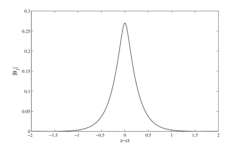
Figure 1. Regular solitary wave obtained numerically by the Petviashili method (dimensionless velocity $V=0.60$).

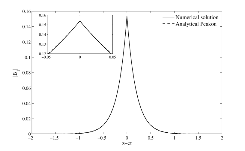
Figure 2. Analytical CH peakon (solid line) and numerical solution (dashed line) obtained by the Petviashili method (dimensionless velocity $V_{1}\approx 0.63$).

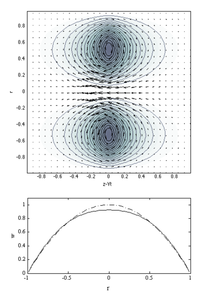
Figure 3. Regular vortexon: (top) streamlines of the perturbation and (bottom) velocity profiles of the perturbed (solid) and laminar (dash) flows.

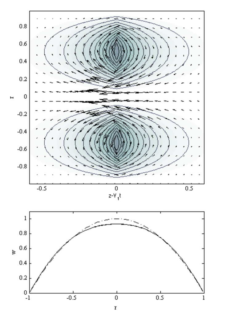
Figure 4. Singular vortexon: (top) streamlines of the perturbation and (bottom) velocity profiles of the perturbed (solid) and laminar (dash) flows.

4.  Conclusions

We investigated the nonlinear dynamics of a disturbance to the laminar state in non-rotating axisymmetric Poiseuille pipe flows. The associated Navier-Stokes equations are projected onto the function space spanned by a finite set of the first few least stable Stokes eigenmodes. The eigenmode amplitudes depend upon both the streamwise direction and time and satisfy a truncated set of coupled generalized CH equations. For the uncoupled equations we found analytically special inviscid travelling waves with wedge-type singularities, viz. peakons, which bifurcate from regular solitary waves as their celerity increase above a well defined threshold. In physical space peakons correspond to localized toroidal vortical structures with discontinuous radial velocities that wrap around the pipe axis (singular centre vortexons). Clearly, the inviscid singular vortexon could be an artifact of the Galerkin truncation of the axisymmetric Euler equations. However, it may be an approximation of singular solutions of the axisymmetric Euler equations (see, for example, [30]) and susceptible to Kelvin-Helmholtz type instability mechanisms. We point out that the inviscid centre vortexon is similar to the neutral mode identified by Walton (2011) [1] and to the inviscid axisymmetric slug structure proposed by Smith et al. (1990) [31]. They may play a role in pipe flow transition as precursors to puffs and slugs, since most likely they are prone to instability by non-axisymmetric disturbances (see [7]).

$$c_{jm}=-\int\limits_{0}^{1}W_{0}\phi_{j}\mathcal{L}\phi_{m}\;r^{-1}\,\mathrm{d}r,\quad\alpha_{jm}=-\int\limits_{0}^{1}\phi_{j}\phi_{m}\;r^{-1}\,\mathrm{d}r,\quad\beta_{jm}=-\int\limits_{0}^{1}W_{0}\phi_{j}\phi_{m}r^{-1}\,\mathrm{d}r,$$

$$F_{jnm}=-\int\limits_{0}^{1}\phi_{j}\left[\partial_{r}\phi_{n}\mathcal{L}\phi_{m}-\partial_{r}\left(\mathcal{L}\phi_{n}\right)\phi_{m}+2r^{-1}\mathcal{L}\phi_{n}\phi_{m}\right]r^{-2}\,\mathrm{d}r,$$

$$H_{jnm}=-\int\limits_{0}^{1}\phi_{j}\phi_{m}\partial_{r}\phi_{n}r^{-2}\,\mathrm{d}r,\quad G_{jnm}=-\int\limits_{0}^{1}\phi_{j}\left[-\phi_{m}\partial_{r}\phi_{n}+2r^{-1}\phi_{n}\phi_{m}\right]r^{-2}\,\mathrm{d}r.$$

References

- [1] A. G. Walton. The stability of developing pipe flow at high Reynolds number and the existence of nonlinear neutral centre modes. J. Fluid Mech., 684:284–315, September 2011.
- [2] B. Hof, A. Juel, and T. Mullin. Scaling of the Turbulence Transition Threshold in a Pipe. Phys. Rev. Lett., 91(24):244502, December 2003.
- [3] P. G. Drazin and W. H. Reid. Hydrodynamic Stability. Cambridge University Press, Cambridge, 2 edition, 2004.
- [4] I. J. Wygnanski and F. H. Champagne. On transition in a pipe. Part 1. The origin of puffs and slugs and the flow in a turbulent slug. J. Fluid Mech., 59(02):281–335, March 1973.
- [5] I. Wygnanski, M. Sokolov, and D. Friedman. On transition in a pipe. Part 2. The equilibrium puff. J. Fluid Mech., 69(02):283–304, March 1975.
- [6] F. T. Smith and R. J. Bodonyi. Amplitude-Dependent Neutral Modes in the Hagen-Poiseuille Flow Through a Circular Pipe. Proc. R. Soc. Lond. A, 384(1787):463–489, December 1982.
- [7] A. G. Walton. The stability of nonlinear neutral modes in Hagen-Poiseuille flow. Proc. R. Soc. Lond. A, 461(2055):813–824, March 2005.
- [8] A. Willis and R. Kerswell. Coherent Structures in Localized and Global Pipe Turbulence. Phys. Rev. Lett., 100(12):124501, March 2008.
- [9] F. Fedele. Travelling waves in axisymmetric pipe flows. Fluid Dynamics Research, 44(4):45509, August 2012.
- [10] S. Leibovich. Axially-symmetric eddies embedded in a rotational stream. J. Fluid Mech., 32(03):529–548, March 1968.
- [11] S. Leibovich. Wave motion and vortex breakdown. In AIAA PAPER 69-645, page 10, 1969.
- [12] S. Leibovich. Weakly non-linear waves in rotating fluids. J. Fluid Mech., 42(04):803–822, March 1970.
- [13] D. J. Benney. Long non-linear waves in fluid flows. J. Math. Phys., 45:52–63, 1966.
- [14] S. Leibovich. Vortex stability and breakdown - Survey and extension. AIAA Journal, 22(9):1192–1206, September 1984.
- [15] O. S. Ryzhov. Solitons in Transitional Boundary Layers. AIAA Journal, 48(2):275–286, 2010.
- [16] Y. S. Kachanov, O. S. Ryzhov, and F. T. Smith. Formation of solitons in transitional boundary layers: theory and experiment. J. Fluid Mech., 251:273–297, April 1993.
- [17] R. Camassa and D. Holm. An integrable shallow water equation with peaked solitons. Phys. Rev. Lett., 71(11):1661–1664, 1993.
- [18] N. Itoh. Nonlinear stability of parallel flows with subcritical Reynolds numbers. Part 2. Stability of pipe Poiseuille flow to finite axisymmetric disturbances. J. Fluid Mech., 82(03):469–479, April 1977.
- [19] F. Fedele, D. L. Hitt, and R. D. Prabhu. Revisiting the stability of pulsatile pipe flow. Eur. J. Mech. B/Fluids, 24(2):237–254, March 2005.
- [20] M. Abramowitz and I. A. Stegun. Handbook of Mathematical Functions. Dover Publications, 1972.
- [21] S. Chen, C. Foias, D. D. Holm, E. Olson, E. S. Titi, and S. Wynne. The Camassa-Holm equations and turbulence in pipes and channels. Phys. D, 133:49–65, 1999.
- [22] J. A. Domaradzki and D. Holm. Navier-Stokes-alpha model: LES equations with nonlinear dispersion. In B Geurts, editor, Modern Simulation Strategies for Turbulent Flow, pages 107–122. 2001.
- [23] C. Foias, D. D. Holm, and E. S. Titi. The Navier-Stokes-alpha model of fluid turbulence. Phys. D, 152-153:505–519, May 2001.
- [24] C. Foias, D. D. Holm, and E. S. Titi. The Three Dimensional Viscous Camassa-Holm Equations, and Their Relation to the Navier-Stokes Equations and Turbulence Theory. J. Dynam. Diff. Eqns., 14(1):1–35, 2002.
- [25] D. Pelinovsky and Y. A. Stepanyants. Convergence of Petviashvili’s iteration method for numerical approximation of stationary solutions of nonlinear wave equations. SIAM J. Num. Anal., 42:1110–1127, 2004.
- [26] T. I. Lakoba and J. Yang. A generalized Petviashvili iteration method for scalar and vector Hamiltonian equations with arbitrary form of nonlinearity. J. Comp. Phys., 226:1668–1692, 2007.
- [27] F. Fedele and D. Dutykh. Hamiltonian form and solitary waves of the spatial Dysthe equations. JETP Lett., 94(12):840–844, October 2011.
- [28] F. Fedele and D. Dutykh. Solitary wave interaction in a compact equation for deep-water gravity waves. JETP Letters, 95(12):622–625, August 2012.
- [29] F. Fedele and D. Dutykh. Special solutions to a compact equation for deep-water gravity waves. J. Fluid Mech, page 15, 2012.
- [30] G. L. Eyink. Dissipative anomalies in singular Euler flows. Phys. D, 237(14-17):1956–1968, August 2008.
- [31] F. T. Smith, D. J. Doorly, and A. P. Rothmayer. On Displacement-Thickness, Wall-Layer and Mid-Flow Scales in Turbulent Boundary Layers, and Slugs of Vorticity in Channel and Pipe Flows. Proc. R. Soc. Lond. A, 428(1875):255–281, April 1990.