Classical FEM-BEM coupling methods:
nonlinearities, well-posedness, and adaptivity

Abstract

We consider a (possibly) nonlinear interface problem in 2D and 3D, which is solved by use of various adaptive FEM-BEM coupling strategies, namely the Johnson-Nédélec coupling, the Bielak-MacCamy coupling, and Costabel’s symmetric coupling. We provide a framework to prove that the continuous as well as the discrete Galerkin solutions of these coupling methods additionally solve an appropriate operator equation with a Lipschitz continuous and strongly monotone operator. Therefore, the coupling formulations are well-defined, and the Galerkin solutions are quasi-optimal in the sense of a Céa-type lemma. For the respective Galerkin discretizations with lowest-order polynomials, we provide reliable residual-based error estimators. Together with an estimator reduction property, we prove convergence of the adaptive FEM-BEM coupling methods. A key point for the proof of the estimator reduction are novel inverse-type estimates for the involved boundary integral operators which are advertized. Numerical experiments conclude the work and compare performance and effectivity of the three adaptive coupling procedures in the presence of generic singularities.

1 Introduction

1.1 Model problem

Let $\Omega\subseteq\mathbb{R}^{d}$ ($d=2,3$) be a bounded Lipschitz domain with polyhedral boundary $\Gamma:=\partial\Omega$ and normal vector $\mathbf{\nu}$. For given data $(f,u_{0},\phi_{0})\in L^{2}(\Omega)\times H^{1/2}(\Gamma)\times H^{-1/2}(\Gamma)$, we consider the nonlinear interface problem

$$-\operatorname{div}(\mathfrak{A}\nabla u) =f \quad\text{in }\Omega,$$ (1a)

$$-\Delta u^{\rm ext} =0 \quad\text{in }\Omega^{\rm ext},$$ (1b)

$$u-u^{\rm ext} =u_{0} \quad\text{on }\Gamma,$$ (1c)

$$(\mathfrak{A}\nabla u-\nabla u^{\rm ext})\cdot\mathbf{\nu} =\phi_{0} \quad\text{on }\Gamma,$$ (1d)

$$u^{\rm ext} =\mathcal{O}(\left\lvert x\right\rvert^{-1}) \quad\text{as }\left\lvert x\right\rvert{}\rightarrow\infty.$$ (1e)

As usual, these equations are understood in the weak sense, i.e. we seek for a solution $(u,u^{\rm ext})\in H^{1}(\Omega)\times H_{\rm loc}^{1}(\Omega^{\rm ext})$, with $H_{\rm loc}^{1}(\Omega^{\rm ext})=\{v\,|\,v\in H^{1}(K)\,,K\subseteq\overline{\Omega^{\rm ext}}\,\text{ compact}\}$, and $\Omega^{\rm ext}:=\mathbb{R}^{d}\backslash\overline{\Omega}$. It is well-known that problem (1) admits a unique solution in 3D. In 2D, the given data have to fulfill the compatibility condition

$$\langle f\hskip 1.42262pt,1\rangle_{\Omega}+\langle\phi_{0}\hskip 1.42262pt,1\rangle_{\Gamma}=0,$$ (2)

to ensure the right behaviour of the solution at infinity. Moreover, in 2D we assume $\operatorname{diam}(\Omega)<1$ to ensure ellipticity of the simple-layer potential $\mathfrak{V}$ defined below. The assumptions on the strongly monotone operator $\mathfrak{A}:\mathbb{R}^{d}\rightarrow\mathbb{R}^{d}$ will be given in Section 2.2. We denote by $H^{1/2}(\Gamma)$ the trace space of $H^{1}(\Omega)$ and by $H^{-1/2}(\Gamma)$ its dual space. For simplicity, we will write $u$ for the trace of a function $u\in H^{1}(\Omega)$, if the meaning is clear.

1.2 Coupling of FEM and BEM

Because of the presence of the unbounded exterior domain $\Omega^{\rm ext}$ in (1b), it is numerically attractive to represent $u^{\rm ext}$ in terms of certain integral operators. This leads to a contribution on the coupling boundary $\Gamma$ instead of the exterior domain $\Omega^{\rm ext}$. For the interior domain $\Omega$ in (1a), the (possible) nonlinearity of $\mathfrak{A}$ as well as the (possible) inhomogeneity $f\neq 0$ favours the use of a finite element approach. This led to the development of certain coupling procedures, and we focus on the Johnson-Nédélec coupling [19], the Bielak-MacCamy coupling [8], and Costabel’s symmetric coupling [13] in the following. All of these approaches lead to a variational formulation

$$b(\mathbf{u},\mathbf{v})=\mathfrak{L}(\mathbf{v})\text{ for all }\mathbf{v}\in\mathcal{H}:=H^{1}(\Omega)\times H^{-1/2}(\Gamma)$$ (3)

with unknown solution $\mathbf{u}\in\mathcal{H}$, which is in a certain sense equivalent to (1). We equip $\mathcal{H}$ with the norm

$$\lVert\mathbf{v}\rVert_{\mathcal{H}}^{2}=\lVert v\rVert_{H^{1}(\Omega)}^{2}+\lVert\psi\rVert_{H^{-1/2}(\Gamma)}^{2}$$ (4)

for $\mathbf{v}=(v,\psi)\in\mathcal{H}$. Here, $b(\cdot,\cdot)$ is a continuous form on $\mathcal{H}\times\mathcal{H}$ which is linear in the second argument, and $\mathfrak{L}(\cdot)$ is a linear and continuous functional on $\mathcal{H}$. The original works [8; 19; 13] focussed on linear $\mathfrak{A}$ and hence bilinear $b(\cdot,\cdot)$, and proved existence and uniqueness of the solution $\mathbf{u}\in\mathcal{H}$ of (3). In the framework of the symmetric coupling well-posedness for nonlinear $\mathfrak{A}$ has first been considered in the pioneering work [12].

For the Galerkin discretization, one considers a finite-dimensional and hence closed subspace $\mathcal{H}_{\ell}$ of $\mathcal{H}$ and seeks $\mathbf{U}_{\ell}\in\mathcal{H}_{\ell}$ such that

$$b(\mathbf{U}_{\ell},\mathbf{V}_{\ell})=\mathfrak{L}(\mathbf{V}_{\ell})\quad\text{for all }\mathbf{V}_{\ell}\in\mathcal{H}_{\ell}.$$ (5)

For linear $\mathfrak{A}$, existence and uniqueness of the Galerkin solution $\mathbf{U}_{\ell}\in\mathcal{H}_{\ell}$ for the symmetric coupling is already found in [13]. Moreover, Galerkin solutions are quasi-optimal in the sense of the Céa-type lemma

$$\lVert\mathbf{u}-\mathbf{U}_{\ell}\rVert_{\mathcal{H}}\leq C_{\mbox{\rm\scriptsize C\'{e}a}}\min_{\mathbf{V}_{\ell}\in\mathcal{H}_{\ell}}\lVert\mathbf{u}-\mathbf{V}_{\ell}\rVert_{\mathcal{H}},$$ (6)

where the constant $C_{\mbox{\rm\scriptsize C\'{e}a}}>0$ depends only on the geometry and on $\mathfrak{A}$, but is independent of the given data, the continuous solution $\mathbf{u}$, and the Galerkin solution $\mathbf{U}_{\ell}$. The analysis of the symmetric coupling has been generalized to nonlinear $\mathfrak{A}$ in [12], but the proof required the underlying mesh to be sufficiently fine, i.e. the maximal mesh-size had to be sufficiently small. Finally, for the nonsymmetric coupling strategies from [8; 19] and even linear problems, the analysis relied on the compactness of a certain integral operator $\mathfrak{K}$ involved. However, this compactness restricted the coupling boundary to be smooth instead of piecewise polynomial.

Only very recently, Sayas [23] proved that the Johnson-Nédélec coupling is equivalent to an elliptic problem, independently of the compactness of $\mathfrak{K}$. For linear $\mathfrak{A}$, more precisely the Yukawa or the Laplace equation, he thus derived that the variational formulation (3) as well as the discrete formulation (5) admit unique solutions and that the discrete solutions are quasi-optimal in the sense of (6). His analysis has been simplified by Steinbach [26]. For quite general linear $\mathfrak{A}$, the latter work introduces a stabilized bilinear form

$$\widetilde{b}(\widetilde{\mathbf{u}},\mathbf{v}):=b(\widetilde{\mathbf{u}},\mathbf{v})+\sigma(\widetilde{\mathbf{u}},\mathbf{v})$$ (7)

which is proved to be elliptic provided the smallest eigenvalue of $\mathfrak{A}$ is larger than $1/4$. Up to some algebraic pre-/postprocessing, the solution $\mathbf{u}$ of (3) coincides with the solution $\widetilde{\mathbf{u}}\in\mathcal{H}$ of

$$\widetilde{b}(\widetilde{\mathbf{u}},\mathbf{v})=\widetilde{\mathfrak{L}}(\mathbf{v})\quad\text{for all }\mathbf{v}\in\mathcal{H},$$ (8)

i.e. $\mathbf{u}=\widetilde{\mathbf{u}}+\mathbf{u}_{0}$. Steinbach thus proposed to approximate the unique solution of (8) by some Galerkin solution $\widetilde{\mathbf{U}}_{\ell}\in\mathcal{H}_{\ell}$ and to obtain an approximation of $\mathbf{u}$ by $\widetilde{\mathbf{U}}_{\ell}+\mathbf{u}_{0}$. One drawback of this method is, however, that the computation of the stabilization $\sigma(\cdot,\cdot)$ as well as of the (constant) offset $\mathbf{u}_{0}$ requires the (numerical) solution of an additional integral equation $\mathfrak{V}\phi_{\rm eq}=1$. Firstly, this might lead to artificial error contributions from generic singularities of $\phi_{\rm eq}$. Secondly, the first Strang lemma comes into play which imposes the assumption that the underlying (boundary) mesh is sufficiently fine.

Finally, we mention the recent work [16], where for the (linear) Yukawa equation ellipticity of the bilinear form $b(\cdot,\cdot)$ is proved for both the Johnson-Nédélec coupling as well as the Bielak-MacCamy coupling.

1.3 A posteriori error estimation

A posteriori error analysis aims to provide computable quantities $\varrho_{\ell}$ which measure the Galerkin error $\lVert\mathbf{u}-\mathbf{U}_{\ell}\rVert_{\mathcal{H}}$ from above (reliability) and below (efficiency). The local information provided by $\varrho_{\ell}$ can then be used to refine the mesh locally, where the Galerkin error appears to be large. For the symmetric coupling, a posteriori error estimation was initiated by [12] for 2D and is well-established since then, cf. e.g. [10; 20; 27] and the references therein. To the best of our knowledge, only residual-based error estimators provide unconditional upper bounds. On the other hand, for this type of estimators the lower bounds still require the mesh to be globally quasi-uniform although efficiency is also observed empirically on locally refined meshes [9]. For the Johnson-Nédélec coupling and the 2D Laplacian, different types of a posteriori error estimators have recently been provided and compared in [5].

1.4 Contributions of current work

Adapting the results and proofs of [16; 23; 26], we present a framework which allows us to prove existence and uniqueness of the three coupling procedures for certain nonlinear $\mathfrak{A}$. Roughly speaking, the idea is as follows: Each form $b(\mathbf{u},\mathbf{v})$ on $\mathcal{H}$ which is linear in $\mathbf{v}$, induces a nonlinear operator $\mathfrak{B}:\mathcal{H}\to\mathcal{H}^{*}$, where $\mathcal{H}^{*}$ denotes the dual space of $\mathcal{H}$. Then, the variational formulation (3) is rewritten in operator formulation

$$\mathfrak{B}\mathbf{u}=\mathfrak{L}.$$ (9)

For each coupling, we introduce an appropriate stabilization $\sigma(\cdot,\cdot)$ and consider the nonlinear operator $\widetilde{\mathfrak{B}}$ induced by $\widetilde{b}(\cdot,\cdot)$ from (7). This is done in a way which ensures equivalence

$$\mathfrak{B}\mathbf{u}=\mathfrak{L}\quad\Longleftrightarrow\quad\widetilde{\mathfrak{B}}\mathbf{u}=\widetilde{\mathfrak{L}}.$$ (10)

Under appropriate assumptions on $\mathfrak{A}$, the operator $\widetilde{\mathfrak{B}}$ is Lipschitz continuous and strongly monotone (or: elliptic). Therefore, the continuous operator formulation $\widetilde{\mathfrak{B}}\mathbf{u}=\widetilde{\mathfrak{L}}$ as well as its Galerkin formulation admit unique solutions $\mathbf{u}\in\mathcal{H}$ resp. $\mathbf{U}_{\ell}\in\mathcal{H}_{\ell}$ which also solve (3) resp. (5) and satisfy the Céa-type estimate (6). For the Johnson-Nédélec coupling and the Bielak-MacCamy coupling, our analysis requires that the ellipticity constant $c_{\rm ell}>0$ of $\mathfrak{A}$ is larger than $1/4$, which reflects the same restriction as for the linear case in [26]. For the symmetric coupling, we avoid any restriction on $c_{\rm ell}>0$. We thus obtain the same results as in [12], but without any restriction on the mesh-size and with a much simpler proof. We stress that, unlike the approach of [26], the stabilized variant is only employed for theoretical reasons to guarantee unique solvability of the non-stabilized equations.

Finally, for lowest-order piecewise polynomials, we derive residual-based a posteriori error estimators which provide reliable upper bounds for the respective Galerkin errors. For the Bielak-MacCamy coupling, we adapt the arguments from our recent preprint [4] to prove that the usual adaptive algorithm drives the residual error estimator to zero.

1.5 Outline

We start with a preliminary Section 2 which collects the precise assumptions on $\mathfrak{A}$, the integral operators $\mathfrak{V}$, $\mathfrak{K}$, and $\mathfrak{W}$ involved, as well as the notation used in the remainder of the paper. Section 3 then considers the Bielak-MacCamy coupling. We sketch the derivation of the coupling equations and prove existence and uniqueness of the continuous as well as of the Galerkin formulation as outlined above. Finally, we state and prove a residual-based a posteriori error estimator. In Section 4 and Section 5, the same is done for the Johnson-Nédélec coupling as well as for Costabel’s symmetric coupling. However, for the sake of brevity and since the proofs are very similar to that of the Bielak-MacCamy coupling, we only sketch the details. Emphasis is laid, however, on the fact that no restriction on the ellipticity constant $c_{\rm ell}>0$ of $\mathfrak{A}$ is imposed in the case of the symmetric coupling. Section 6 states the usual adaptive mesh-refining algorithm. Using the concept of estimator reduction and recent results of [4], convergence of $\mathbf{U}_{\ell}$ to $\mathbf{u}$ is proved as $\ell\to\infty$, where $\ell$ denotes the step counter of the adaptive loop. A final Section 7 provides some numerical experiments. Emphasis is laid on the comparison of the three coupling procedures with respect to accuracy and computational time. Moreover, we numerically investigate the restriction $c_{\rm ell}>1/4$ in case of the Johnson-Nédélec and Bielak-MacCamy coupling. Finally, we see that the proposed adaptive schemes are much superior to the usual approach, where the mesh is only uniformly refined.

2 Preliminaries

2.1 Boundary integral operators

Throughout, $\mathfrak{K}$ denotes the double-layer potential with adjoint $\mathfrak{K}^{\dagger}$, $\mathfrak{V}$ denotes the simple-layer potential, and $\mathfrak{W}$ the hypersingular operator. With the fundamental solution of the Laplacian

$$G(z):=\begin{cases}-\tfrac{1}{2\pi}\log\left\lvert z\right\rvert&\quad\text{for }z\in\mathbb{R}^{2}\backslash\{0\},\\ \frac{1}{4\pi}\frac{1}{\left\lvert z\right\rvert}&\quad\text{for }z\in\mathbb{R}^{3}\backslash\{0\},\end{cases}$$

these integral operators formally read as follows,

$$(\mathfrak{V}\varphi)(x) =\int_{\Gamma}G(x-y)\varphi(y)\,d\Gamma_{y},$$

$$(\mathfrak{K}\varphi)(x) =\int_{\Gamma}\partial_{\mathbf{\nu}(y)}G(x-y)\varphi(y)\,d\Gamma_{y},$$

$$(\mathfrak{W}\varphi)(x) =-\partial_{\mathbf{\nu}(x)}\int_{\Gamma}\partial_{\mathbf{\nu}(y)}G(x-y)\varphi(y)\,d\Gamma_{y},$$

for $x\in\Gamma$ and with $\partial_{\mathbf{\nu}(y)}$ denoting the normal derivative at $y\in\Gamma$. By continuous extension, we obtain bounded linear operators

$$\begin{split}\mathfrak{V}&\in L(H^{-1/2}(\Gamma);H^{1/2}(\Gamma)),\\ \mathfrak{K}&\in L(H^{1/2}(\Gamma);H^{1/2}(\Gamma)),\\ \mathfrak{K}^{\dagger}&\in L(H^{-1/2}(\Gamma);H^{-1/2}(\Gamma)),\\ \mathfrak{W}&\in L(H^{1/2}(\Gamma);H^{-1/2}(\Gamma)).\end{split}$$ (11)

Finally, we stress the ellipticity of the simple-layer potential $\langle\phi\hskip 1.42262pt,\mathfrak{V}\phi\rangle_{\Gamma}\gtrsim\lVert\phi\rVert_{H^{-1/2}(\Gamma)}^{2}$. Together with symmetry and continuity of $\mathfrak{V}$, this implies norm equivalence $\langle\phi\hskip 1.42262pt,\mathfrak{V}\phi\rangle_{\Gamma}\simeq\lVert\phi\rVert_{H^{-1/2}(\Gamma)}^{2}$. For further properties of the integral operators, the reader is referred to the literature, e.g. the monographs [18; 21; 22; 25].

2.2 Strongly monotone operators

An operator $\widetilde{\mathfrak{B}}:\mathcal{H}\to\mathcal{H}^{*}$ is Lipschitz continuous provided that there is a constant $C_{\rm Lip}>0$ such that

$$\|\widetilde{\mathfrak{B}}\mathbf{u}-\widetilde{\mathfrak{B}}\mathbf{v}\|_{\mathcal{H}^{*}}\leq C_{\rm Lip}\lVert\mathbf{u}-\mathbf{v}\rVert_{\mathcal{H}}$$ (12)

holds for all $\mathbf{u},\mathbf{v}\in\mathcal{H}$, where $\|\cdot\|_{\mathcal{H}^{*}}$ denotes the usual norm on the dual space $\mathcal{H}^{*}$. With $\langle\cdot\hskip 1.42262pt,\cdot\rangle$ the duality brackets on $\mathcal{H}^{*}\times\mathcal{H}$, the operator $\widetilde{\mathfrak{B}}$ is strongly monotone provided that there is a constant $C_{\rm ell}>0$ such that

$$\langle\widetilde{\mathfrak{B}}\mathbf{u}-\widetilde{\mathfrak{B}}\mathbf{v}\hskip 1.42262pt,\mathbf{u}-\mathbf{v}\rangle\geq C_{\rm ell}\,\lVert\mathbf{u}-\mathbf{v}\rVert_{\mathcal{H}}^{2}$$ (13)

holds for all $\mathbf{u},\mathbf{v}\in\mathcal{H}$. We refer to [29, Section 25.4] for the following standard results on strongly monotone operators: Under (12)–(13), the operator $\widetilde{\mathfrak{B}}$ is bijective, and the inverse $\widetilde{\mathfrak{B}}^{-1}$ is Lipschitz continuous with Lipschitz constant $1/C_{\rm ell}$. Consequently, for every $\widetilde{\mathfrak{L}}\in\mathcal{H}^{*}$, there is a unique $\mathbf{u}\in\mathcal{H}$ with

$$\langle\widetilde{\mathfrak{B}}\mathbf{u}\hskip 1.42262pt,\mathbf{v}\rangle=\widetilde{\mathfrak{L}}(\mathbf{v})\quad\text{for all }\mathbf{v}\in\mathcal{H},$$ (14)

and $\mathbf{u}$ depends Lipschitz continuously on $\widetilde{\mathfrak{L}}$. Moreover, for every closed subspace $\mathcal{H}_{\ell}$ of $\mathcal{H}$, there is a unique $\mathbf{U}_{\ell}\in\mathcal{H}_{\ell}$ such that

$$\langle\widetilde{\mathfrak{B}}\mathbf{U}_{\ell}\hskip 1.42262pt,\mathbf{V}_{\ell}\rangle=\widetilde{\mathfrak{L}}(\mathbf{V}_{\ell})\quad\text{for all }\mathbf{V}_{\ell}\in\mathcal{H}_{\ell}.$$ (15)

Finally, $\mathbf{U}_{\ell}$ depends also Lipschitz continuously on $\widetilde{\mathfrak{L}}$, and there holds the Céa-type quasi-optimality (6), where $C_{\mbox{\rm\scriptsize C\'{e}a}}=C_{\rm Lip}/C_{\rm ell}$.

Remark 1

Provided that the discrete spaces $\mathcal{H}_{\ell}$ satisfy

$$\mathcal{H}_{\ell}\subseteq\mathcal{H}_{\ell+1}\text{ for all }\ell\geq 0\quad\text{and}\quad\overline{\mbox{$\bigcup_{\ell=0}^{\infty}$}\mathcal{H}_{\ell}}=\mathcal{H},$$ (16)

the quasi-optimality (6) implies convergence $\mathbf{U}_{\ell}\to\mathbf{u}$ of the Galerkin solutions as $\ell\to\infty$. In practice, the conditions (16) are satisfied if the underlying meshes are successively refined and the corresponding mesh-sizes tend to zero everywhere.

To apply the framework of strongly monotone operators to the FEM-BEM coupling formulations presented in Section 3, 4, and 5, we have to make some assumptions on the coefficient function $\mathfrak{A}:\mathbb{R}^{d}\rightarrow\mathbb{R}^{d}$. Firstly, we consider $\mathfrak{A}$ to be Lipschitz continuous, i.e. there exists a constant $c_{\rm lip}$ such that

$$|\mathfrak{A}y-\mathfrak{A}z|\leq c_{\rm lip}|y-z|$$ (17)

holds for all $y,z\in\mathbb{R}^{d}$. Integrating the square of (17), one obtains

$$\lVert\mathfrak{A}\nabla v-\mathfrak{A}\nabla w\rVert_{L^{2}(\Omega)}^{2}\leq c_{\rm lip}^{2}\lVert\nabla v-\nabla w\rVert_{L^{2}(\Omega)}^{2}$$ (18)

for all $v,w\in H^{1}(\Omega)$. Secondly, we assume $\mathfrak{A}$ to be strongly monotone in the following sense: There exists a constant $c_{\rm ell}>0$ such that there holds

$$c_{\rm ell}\lVert\nabla v-\nabla w\rVert_{L^{2}(\Omega)}^{2}\leq\langle\mathfrak{A}\nabla v-\mathfrak{A}\nabla w\hskip 1.42262pt,\nabla v-\nabla w\rangle_{\Omega}$$ (19)

for all $v,w\in H^{1}(\Omega)$. Here, $\langle\cdot\hskip 1.42262pt,\cdot\rangle_{\Omega}$ denotes the $L^{2}(\Omega)$-scalar product, i.e. $\langle v\hskip 1.42262pt,w\rangle_{\Omega}=\int_{\Omega}vw\,dx$. Similarly, we shall write $\langle\cdot\hskip 1.42262pt,\cdot\rangle_{\Gamma}$ for the $L^{2}(\Gamma)$-scalar product which is extended by continuity to the duality bracket between $H^{1/2}(\Gamma)$ and $H^{-1/2}(\Gamma)$.

Remark 2

We stress that conditions (18) and (19) are sufficient for solvability considerations, see Sections 3.2–3.3, 4.2–4.3, and 5.2–5.3. Anyhow, in our a posteriori analysis we need that $\mathfrak{A}$ is pointwise Lipschitz continuous (17).

Remark 3

As far as existence and uniqueness of continuous solution $\mathbf{u}$ and discrete solution $\mathbf{U}_{\ell}$ from (14)–(15) is concerned, our analysis only requires that the induced operator $\widetilde{\mathfrak{B}}$ is strictly monotone, i.e.

$$\langle\widetilde{\mathfrak{B}}\mathbf{u}\!-\!\widetilde{\mathfrak{B}}\mathbf{v}\hskip 1.42262pt,\mathbf{u}\!-\!\mathbf{v}\rangle>0\text{ for all }\mathbf{u},\mathbf{v}\in\mathcal{H}\text{ with }\mathbf{u}\neq\mathbf{v},$$ (20)

i.e. (13) is replaced by (20). Then, the Browder-Minty theorem applies and, in particular, proves weak convergence $\mathbf{U}_{\ell}\rightharpoonup\mathbf{u}$ in $\mathcal{H}$ as $\ell\to\infty$ under assumption (16). In this framework, however, the Céa-type estimate (6) cannot hold in general and a posteriori error estimates can hardly been derived. Therefore, we leave the details to the reader. However, we stress that (20) holds if the nonlinearity $\mathfrak{A}$ satisfies

$$0<\langle\mathfrak{A}\nabla v-\mathfrak{A}\nabla w\hskip 1.42262pt,\nabla v-\nabla w\rangle_{\Omega}$$ (21)

for all $v,w\in H^{1}(\Omega)$ with $\nabla v\neq\nabla w$ instead of (19).

2.3 Discrete spaces

In Sections 3–5, the model problem (1) is reformulated as variational equality (3) in the Hilbert space $\mathcal{H}:=H^{1}(\Omega)\times H^{-1/2}(\Gamma)$. For the respective discretizations, let $\mathcal{T}_{\ell}$ be a regular triangulation of $\Omega$ and let $\mathcal{E}_{\ell}^{\Gamma}$ be a regular triangulation of $\Gamma$, where regularity is understood in the sense of Ciarlet. We approximate a function $u\in H^{1}(\Omega)$ by continuous, $\mathcal{T}_{\ell}$-piecewise affine functions on $\Omega$. For a function $\phi\in H^{-1/2}(\Gamma)$, we use $\mathcal{E}_{\ell}^{\Gamma}$-piecewise constant functions, i.e. our discrete spaces read $\mathcal{H}_{\ell}:=\SS^{1}(\mathcal{T}_{\ell})\times\mathcal{P}^{0}(\mathcal{E}_{\ell}^{\Gamma})\subseteq\mathcal{H}$.

Let $\mathcal{E}_{\ell}^{\Omega}$ denote the set of all interior faces, i.e. for $E\in\mathcal{E}_{\ell}^{\Omega}$ there exist unique elements $T^{+},T^{-}$ with $E=T^{+}\cap T^{-}$. We define the patch of $E\in\mathcal{E}_{\ell}^{\Omega}$ by $\omega_{\ell,E}:=T^{+}\cup T^{-}$. Furthermore, we define the local mesh-width function $h_{\ell}$ by

$$h_{\ell}(\tau):=\begin{cases}\lvert\tau\rvert^{1/d}&\quad\text{for }\tau\in\mathcal{T}_{\ell},\\ \lvert\tau\rvert^{1/(d-1)}&\quad\text{for }\tau\in\mathcal{E}_{\ell}^{\Omega}\cup\mathcal{E}_{\ell}^{\Gamma},\end{cases}$$

where $\lvert\cdot\rvert$ denotes the volume resp. surface measure. A triangulation $\mathcal{T}_{\ell}$ is called $\gamma$-shape regular, if there holds

$$\sigma(\mathcal{T}_{\ell}):=\max\limits_{T\in\mathcal{T}_{\ell}}\frac{\operatorname{diam}(T)^{d}}{|T|}\leq\gamma.$$ (22)

Analogously we call $\mathcal{E}_{\ell}^{\Gamma}$ $\gamma$-shape regular, if

$$\sigma(\mathcal{E}_{\ell}^{\Gamma}):=\max\limits_{E\in\mathcal{E}_{\ell}^{\Gamma}}\frac{\operatorname{diam}(E)^{2}}{|E|}\leq\gamma,$$ (23)

for $d=3$. For $d=2$, the $\gamma$-shape regularity of $\mathcal{E}_{\ell}^{\Gamma}$ reads

$$\sigma(\mathcal{E}_{\ell}^{\Gamma}):=\max\limits_{E\neq E^{\prime}}\left\{\frac{\left\lvert E^{\prime}\right\rvert}{\left\lvert E\right\rvert}\,\middle|\,E^{\prime}\cap E\neq\emptyset\right\}\leq\gamma.$$ (24)

The definition of $h_{\ell}$ and shape regularity implies equivalence $\operatorname{diam}(\tau)\simeq h_{\ell}(\tau)\simeq h_{\ell}(\tau^{\prime})$ for all $\tau,\tau^{\prime}\in\mathcal{T}_{\ell}$ resp. $\tau,\tau^{\prime}\in\mathcal{E}_{\ell}^{\Gamma}$ with $\tau\cap\tau^{\prime}\neq\emptyset$, where the hidden constants depend only on $\gamma$.

Remark 4

(i) We stress that $\mathcal{T}_{\ell}$ and $\mathcal{E}_{\ell}^{\Gamma}$ are formally independent triangulations of $\Omega$ and $\Gamma$, respectively. For the numerical implementation, however, we restrict to the case that $\mathcal{E}_{\ell}^{\Gamma}$ is the restriction $\mathcal{T}_{\ell}|_{\Gamma}$ of $\mathcal{T}_{\ell}$ on the boundary, which indeed is a regular triangulation of $\Gamma$. In this case, we finally remark that $\gamma$-shape regularity of $\mathcal{T}_{\ell}$ also implies $\widetilde{\gamma}$-shape regularity of $\mathcal{E}_{\ell}^{\Gamma}:=\mathcal{T}_{\ell}|_{\Gamma}$.
(ii) In 2D, the radiation condition (1e) of $u^{\rm ext}$ can also be adapted to $u^{\rm ext}(x)=a\log|x|+\mathcal{O}(1)$ for $x\rightarrow\infty$ and fixed $a\in\mathbb{R}$. In this case, the compatibility condition (2) can be dropped. The analysis of the following sections still holds true for that case.

3 Bielak-MacCamy coupling

We can reformulate problem (1) with the help of the Bielak-MacCamy FEM-BEM coupling, which first appeared in [8]. This section is build up as follows: Firstly, we give a short sketch of the derivation of the Bielak-MacCamy coupling equations. Then, we investigate well-posedness of their continuous and discrete formulations. And last, we derive an residual-based error estimator for the Bielak-MacCamy coupling method.

3.1 Derivation of Bielak-MacCamy coupling

The first Green’s formula for the interior part (1a) reads

$$\langle\mathfrak{A}\nabla u\hskip 1.42262pt,\nabla v\rangle_{\Omega}-\langle\mathfrak{A}\nabla u\cdot\mathbf{\nu}\hskip 1.42262pt,v\rangle_{\Gamma}=\langle f\hskip 1.42262pt,v\rangle_{\Omega}$$ (25)

for all $v\in H^{1}(\Omega)$. We plug in the jump condition (1d) for the normal derivative and obtain

$$\langle\mathfrak{A}\nabla u\hskip 1.42262pt,\nabla v\rangle_{\Omega}\!-\!\langle\nabla u^{\rm ext}\cdot\mathbf{\nu}\hskip 1.42262pt,v\rangle_{\Gamma}=\langle f\hskip 1.42262pt,v\rangle_{\Omega}\!+\!\langle\phi_{0}\hskip 1.42262pt,v\rangle_{\Gamma}.$$ (26)

For the exterior solution $u^{\rm ext}$ of (1b), we make an indirect potential ansatz with the simple-layer potential

$$u^{\rm ext}=\widetilde{\mathfrak{V}}\phi\quad\text{in }\Omega^{\rm ext},$$ (27)

where the integral operator $\widetilde{\mathfrak{V}}$ is defined as $\mathfrak{V}$, but is now evaluated in $\Omega^{\rm ext}$ instead of $\Gamma$. We stress that the density $\phi\in H^{-1/2}(\Gamma)$ is unknown. Then, we use properties of the simple-layer potential operator: Firstly, by use of the continuity of the simple-layer potential in $\mathbb{R}^{d}$, i.e. $\widetilde{\mathfrak{V}}\phi=\mathfrak{V}\phi$ on $\Gamma$, and the trace jump condition (1c), we see

$$-u+\mathfrak{V}\phi=-u_{0}\quad\text{on }\Gamma.$$ (28)

Secondly, we use the jump condition of the exterior conormal derivative of the simple-layer potential to see

$$\nabla u^{\rm ext}\cdot\mathbf{\nu}=\partial_{\mathbf{\nu}}^{\rm ext}\widetilde{\mathfrak{V}}\phi=-(\tfrac{1}{2}-\mathfrak{K}^{\dagger})\phi.$$ (29)

Plugging the last equation into (26) and supplementing the system with the variational formulation of (28), we end up with the variational formulation of the Bielak-MacCamy coupling: Find $\mathbf{u}=(u,\phi)\in\mathcal{H}$ such that

$$\langle\mathfrak{A}\nabla u\hskip 1.42262pt,\nabla v\rangle_{\Omega}+\langle(\tfrac{1}{2}-\mathfrak{K}^{\dagger})\phi\hskip 1.42262pt,v\rangle_{\Gamma} =\langle f\hskip 1.42262pt,v\rangle_{\Omega}+\langle\phi_{0}\hskip 1.42262pt,v\rangle_{\Gamma},$$

$$-\langle\psi\hskip 1.42262pt,u\rangle_{\Gamma}+\langle\psi\hskip 1.42262pt,\mathfrak{V}\phi\rangle_{\Gamma} =-\langle\psi\hskip 1.42262pt,u_{0}\rangle_{\Gamma},$$ (30)

holds for all $\mathbf{v}=(v,\psi)\in\mathcal{H}$.

From now on, let $\mathcal{X}_{\ell}$ be a closed subspace of $H^{1}(\Omega)$ and $\mathcal{Y}_{\ell}$ be a closed subspace of $H^{-1/2}(\Gamma)$. We define $\mathcal{H}_{\ell}:=\mathcal{X}_{\ell}\times\mathcal{Y}_{\ell}$. Note that the entire space $\mathcal{H}=\mathcal{H}_{\ell}$ is a valid choice, and hence the following analysis applies to both, the continuous formulation (30) and the Galerkin discretization. In the latter case, $\mathbf{u}\in\mathcal{H}$ in (30) is replaced by $\mathbf{U}_{\ell}\in\mathcal{H}_{\ell}$, and $\mathbf{v}\in\mathcal{H}$ is replaced by arbitrary $\mathbf{V}_{\ell}\in\mathcal{H}_{\ell}$.

3.2 Stabilization

We define the linear form $b_{{\rm bmc}}:\mathcal{H}\times\mathcal{H}\rightarrow\mathbb{R}$ for any $\mathbf{u}=(u,\phi),\mathbf{v}=(v,\psi)\in\mathcal{H}$ by

$$\begin{split}b_{{\rm bmc}}(\mathbf{u},\mathbf{v}):=\langle\mathfrak{A}\nabla u\hskip 1.42262pt,\nabla v\rangle_{\Omega}&+\langle(\tfrac{1}{2}-\mathfrak{K}^{\dagger})\phi\hskip 1.42262pt,v\rangle_{\Gamma}\\ &-\langle\psi\hskip 1.42262pt,u\rangle_{\Gamma}+\langle\psi\hskip 1.42262pt,\mathfrak{V}\phi\rangle_{\Gamma}.\end{split}$$ (31)

Note that $b_{{\rm bmc}}(\cdot,\cdot)$ is only linear in the second argument. Furthermore, we define linear functionals $a_{1}$ and $a_{2}$ on $H^{1}(\Omega)$ and $H^{-1/2}(\Gamma)$ by

$$a_{1}(v) :=\langle f\hskip 1.42262pt,v\rangle_{\Omega}+\langle\phi_{0}\hskip 1.42262pt,v\rangle_{\Gamma}$$ (32)

$$a_{2}(\psi) :=\langle\psi\hskip 1.42262pt,-u_{0}\rangle_{\Gamma}$$ (33)

for all $\mathbf{v}=(v,\psi)\in\mathcal{H}$. For $a_{2}$, we also use the notation $a_{2}(\psi)=\langle\psi\hskip 1.42262pt,a_{2}\rangle_{\Gamma}$. With these definitions, the continuous formulation of the Bielak-MacCamy coupling is equivalently written as follows: Find $\mathbf{u}\in\mathcal{H}$ such that

$$b_{{\rm bmc}}(\mathbf{u},\mathbf{v})=\mathfrak{L}(\mathbf{v}):=a_{1}(v)+a_{2}(\psi)$$ (34)

for all $\mathbf{v}\in\mathcal{H}$. Moreover, the Galerkin formulation of problem (30) reads: Find $\mathbf{U}_{\ell}\in\mathcal{H}_{\ell}$ such that

$$b_{{\rm bmc}}(\mathbf{U}_{\ell},\mathbf{V}_{\ell})=\mathfrak{L}(\mathbf{V}_{\ell})$$ (35)

holds for all $\mathbf{V}_{\ell}=(V_{\ell},\Psi_{\ell})\in\mathcal{H}_{\ell}$.

Throughout the remainder of this section, we need the following assumption.

Assumption 5

There is a fixed function $\xi\in\bigcap_{\ell\in\mathbb{N}_{0}}\mathcal{Y}_{\ell}$ with $\langle\xi\hskip 1.42262pt,1\rangle_{\Gamma}\neq 0$.

Remark 6

The discrete space $\mathcal{Y}_{\ell}=\mathcal{P}^{0}(\mathcal{E}_{\ell}^{\Gamma})$, introduced in Section 2.3, fulfills Assumption 5 with $\xi=1$.

Now, we try to show ellipticity of a linear form which is equivalent to $b_{{\rm bmc}}(\cdot,\cdot)$. Firstly, note that we have to take care of the fact that $b_{{\rm bmc}}(\cdot,\cdot)$ is not elliptic since

$$b_{{\rm bmc}}((1,0),(1,0))=\langle\mathfrak{A}\nabla 1\hskip 1.42262pt,\nabla 1\rangle_{\Omega}=0.$$ (36)

Therefore, we introduce a new linear form $\widetilde{b}_{{\rm bmc}}(\cdot,\cdot)$ which is equivalent to $b_{{\rm bmc}}(\cdot,\cdot)$.

Theorem 7

With $\xi$ from Assumption 5, the linear form

$$\begin{split}\widetilde{b}_{{\rm bmc}}(\mathbf{U}_{\ell},\mathbf{V}_{\ell})&:=b_{{\rm bmc}}(\mathbf{U}_{\ell},\mathbf{V}_{\ell})\\ &\quad+\langle\xi\hskip 1.42262pt,\mathfrak{V}\Phi_{\ell}-U_{\ell}\rangle_{\Gamma}\langle\xi\hskip 1.42262pt,\mathfrak{V}\Psi_{\ell}-V_{\ell}\rangle_{\Gamma}\end{split}$$ (37)

is equivalent to the linear form $b_{{\rm bmc}}(\cdot,\cdot)$ in the following sense: The pair $\mathbf{U}_{\ell}=(U_{\ell},\Phi_{\ell})\in\mathcal{H}_{\ell}$ solves problem (35) if and only if it solves

$$\widetilde{b}_{{\rm bmc}}(\mathbf{U}_{\ell},\mathbf{V}_{\ell})=\mathfrak{L}(\mathbf{V}_{\ell})+\langle\xi\hskip 1.42262pt,a_{2}\rangle_{\Gamma}\langle\xi\hskip 1.42262pt,\mathfrak{V}\Psi_{\ell}-V_{\ell}\rangle_{\Gamma}$$ (38)

for all $\mathbf{V}_{\ell}=(V_{\ell},\Psi_{\ell})\in\mathcal{H}_{\ell}$.

Proof

Step 1. Let $\mathbf{U}_{\ell}=(U_{\ell},\Phi_{\ell})$ be a solution of (34). Testing with $(V_{\ell},\Psi_{\ell})=(0,\xi)\in\mathcal{H}_{\ell}$, we see $b_{{\rm bmc}}(\mathbf{U}_{\ell},(0,\xi))$$=a_{2}(\xi)$. With the definition of $b_{{\rm bmc}}(\cdot,\cdot)$, we infer

$$0=b_{{\rm bmc}}(\mathbf{U}_{\ell},(0,\xi))-a_{2}(\xi)=\langle\xi\hskip 1.42262pt,\mathfrak{V}\Phi_{\ell}-U_{\ell}-a_{2}\rangle_{\Gamma}.$$

Hence, $\langle\xi\hskip 1.42262pt,\mathfrak{V}\Phi_{\ell}-U_{\ell}-a_{2}\rangle_{\Gamma}\langle\xi\hskip 1.42262pt,\mathfrak{V}\Psi_{\ell}-V_{\ell}\rangle_{\Gamma}=0$ for all $\mathbf{V}_{\ell}\in\mathcal{H}_{\ell}$. Clearly, this is equivalent to

$$\langle\xi\hskip 1.42262pt,\mathfrak{V}\Phi_{\ell}-U_{\ell}\rangle_{\Gamma}\langle\xi\hskip 1.42262pt,\mathfrak{V}\Psi_{\ell}-V_{\ell}\rangle_{\Gamma}=\langle\xi\hskip 1.42262pt,a_{2}\rangle_{\Gamma}\langle\xi\hskip 1.42262pt,\mathfrak{V}\Psi_{\ell}-V_{\ell}\rangle_{\Gamma}$$

for all $\mathbf{V}_{\ell}=(V_{\ell},\Psi_{\ell})\in\mathcal{H}_{\ell}$. Therefore, $\mathbf{U}_{\ell}=(U_{\ell},\Phi_{\ell})\in\mathcal{H}_{\ell}$ also solves problem (38).
Step 2. For the converse implication, let $\mathbf{U}_{\ell}=(U_{\ell},\Phi_{\ell})\in\mathcal{H}_{\ell}$ solve (38). The choice of $\mathbf{V}_{\ell}=(0,\xi)$ in (38) gives

$$a_{2}(\xi) +\langle\xi\hskip 1.42262pt,a_{2}\rangle_{\Gamma}\langle\xi\hskip 1.42262pt,\mathfrak{V}\xi\rangle_{\Gamma}=\widetilde{b}_{{\rm bmc}}((U_{\ell},\Phi_{\ell}),(0,\xi))$$

$$=\langle\xi\hskip 1.42262pt,\mathfrak{V}\Phi_{\ell}-U_{\ell}\rangle_{\Gamma}+\langle\xi\hskip 1.42262pt,\mathfrak{V}\Phi_{\ell}-U_{\ell}\rangle_{\Gamma}\langle\xi\hskip 1.42262pt,\mathfrak{V}\xi\rangle_{\Gamma},$$

which is equivalent to

$$\langle\xi\hskip 1.42262pt,\mathfrak{V}\Phi_{\ell}-U_{\ell}-a_{2}\rangle_{\Gamma}(1+\langle\xi\hskip 1.42262pt,\mathfrak{V}\xi\rangle_{\Gamma})=0.$$

Since $\mathfrak{V}$ is $H^{-1/2}(\Gamma)$-elliptic, the last equation implies $\langle\xi\hskip 1.42262pt,\mathfrak{V}\Phi_{\ell}-U_{\ell}-a_{2}\rangle=0$. We thus infer

$$\widetilde{b}_{{\rm bmc}}(\mathbf{U}_{\ell},\mathbf{V}_{\ell})-b_{{\rm bmc}}(\mathbf{U}_{\ell},\mathbf{V}_{\ell})$$

$$\quad=\langle\xi\hskip 1.42262pt,\mathfrak{V}\Phi_{\ell}-U_{\ell}\rangle_{\Gamma}\langle\xi\hskip 1.42262pt,\mathfrak{V}\Psi_{\ell}-V_{\ell}\rangle_{\Gamma}$$

$$\quad=\langle\xi\hskip 1.42262pt,a_{2}\rangle_{\Gamma}\langle\xi\hskip 1.42262pt,\mathfrak{V}\Psi_{\ell}-V_{\ell}\rangle_{\Gamma}$$

which, together with (37) and (38), proves that $\mathbf{U}_{\ell}=(U_{\ell},\Phi_{\ell})$ is also a solution of problem (34). ∎

3.3 Existence and uniqueness of solutions

The linear forms $b_{{\rm bmc}}(\cdot,\cdot)$ and $\widetilde{b}_{{\rm bmc}}(\cdot,\cdot)$ induce operators $\mathfrak{B}_{{\rm bmc}},\widetilde{\mathfrak{B}}_{{\rm bmc}}:\mathcal{H}\rightarrow\mathcal{H}^{*}$ by

$$\begin{split}\langle\mathfrak{B}_{{\rm bmc}}\mathbf{u}\hskip 1.42262pt,\mathbf{v}\rangle&:=b_{{\rm bmc}}(\mathbf{u},\mathbf{v})\quad\text{for all }\mathbf{u},\mathbf{v}\in\mathcal{H},\\ \langle\widetilde{\mathfrak{B}}_{{\rm bmc}}\mathbf{u}\hskip 1.42262pt,\mathbf{v}\rangle&:=\widetilde{b}_{{\rm bmc}}(\mathbf{u},\mathbf{v})\quad\text{for all }\mathbf{u},\mathbf{v}\in\mathcal{H}.\end{split}$$ (39)

The main result of this section reads as follows:

Theorem 8

Under Assumption 5 and provided that the ellipticity constant $c_{\rm ell}$ of $\mathfrak{A}$ fulfills $c_{\rm ell}>1/4$, the operator $\widetilde{\mathfrak{B}}_{{\rm bmc}}$ is strongly monotone and Lipschitz continuous.

The proof requires the following lemma which is proved by means of a Rellich compactness argument.

Lemma 9

For $\mathbf{u}=(u,\phi)\in\mathcal{H}$, let

$$|\!|\!|\mathbf{u}\,\!|\!|\!|^{2}:=\lVert\nabla u\rVert_{L^{2}(\Omega)}^{2}+\langle\phi\hskip 1.42262pt,\mathfrak{V}\phi\rangle_{\Gamma}+\lvert\langle\xi\hskip 1.42262pt,\mathfrak{V}\phi-u\rangle_{\Gamma}\rvert^{2},$$ (40)

where $\xi$ is provided by Assumption 5. Then, $|\!|\!|\cdot\,\!|\!|\!|$ defines an equivalent norm on $\mathcal{H}$.

Proof

Clearly, there holds $|\!|\!|\mathbf{u}\,\!|\!|\!|\lesssim\lVert\mathbf{u}\rVert_{\mathcal{H}}$ for all $\mathbf{u}=(u,\phi)\\ \in\mathcal{H}$. To see the converse estimate, we argue by contradiction and assume that $\lVert\mathbf{u}_{n}\rVert_{\mathcal{H}}>n|\!|\!|\mathbf{u}_{n}\,\!|\!|\!|$ for certain $\mathbf{u}_{n}=(u_{n},\phi_{n})$ and all $n\in\mathbb{N}$. We define $\mathbf{v}_{n}=(v_{n},\psi_{n})$ by

$$\mathbf{v}_{n}:=\frac{\mathbf{u}_{n}}{\lVert\mathbf{u}_{n}\rVert_{\mathcal{H}}}$$

and obtain $\lVert(v_{n},\psi_{n})\rVert_{\mathcal{H}}=1$ as well as $|\!|\!|(v_{n},\psi_{n})\,\!|\!|\!|<1/n$. By definition of $|\!|\!|\cdot\,\!|\!|\!|$ and ellipticity of $\mathfrak{V}$, this implies $\psi_{n}\rightarrow 0\in H^{-1/2}(\Gamma)$ and $\nabla v_{n}\rightarrow 0\in L^{2}(\Omega)$. Moreover, by extracting a subsequence, we may assume that $(v_{n},\psi_{n})\rightharpoonup(v,\psi)$ in $\mathcal{H}$. Clearly, this implies $\psi=0$ and $v_{n}\rightharpoonup v\in H^{1}(\Omega)$, whence $v_{n}\rightarrow v\in L^{2}(\Omega)$. Moreover, weak lower semi-continuity of $|\!|\!|\cdot\,\!|\!|\!|$ implies $|\!|\!|(v,\psi)\,\!|\!|\!|=0$, whence $\nabla v=0$ and $|\langle\xi\hskip 1.42262pt,v\rangle_{\Gamma}|=0$. From the choice of $\xi$ and since $v$ is constant, we infer $v=0$ and thus $v_{n}\rightarrow 0\in H^{1}(\Omega)$. Altogether, $\mathbf{v}_{n}=(v_{n},\psi_{n})\rightarrow 0\in\mathcal{H}$ contradicts $\lVert\mathbf{v}_{n}\rVert_{\mathcal{H}}=1$.∎

The following proof of Theorem 8 is very much influenced by the investigations of [23; 26]. We recall some basic facts on the boundary integral operators, cf. e.g. [25, Chapter 6]: For given $\chi\in H^{-1/2}(\Gamma)$, let $u_{*}=\widetilde{\mathfrak{V}}\chi$. Then there holds

• $\partial_{\mathbf{\nu}}u_{*}=(\tfrac{1}{2}+\mathfrak{K}^{\dagger})\chi$,

• $\langle\partial_{\mathbf{\nu}}u_{*}\hskip 1.42262pt,v\rangle_{\Gamma}=\langle\nabla u_{*}\hskip 1.42262pt,\nabla v\rangle_{\Omega}$ for all $v\in H^{1}(\Omega)$,

• $\langle\chi\hskip 1.42262pt,\mathfrak{V}\chi\rangle_{\Gamma}=\langle[\partial_{\mathbf{\nu}}u_{*}]\hskip 1.42262pt,\mathfrak{V}\chi\rangle_{\Gamma}=\lVert\nabla u_{*}\rVert_{L^{2}(\mathbb{R}^{d})}^{2}$,

where the last equation is only valid for $d=2$, if $\chi\in H_{*}^{-1/2}(\Gamma)=\left\{\psi\in H^{-1/2}(\Gamma)\,\middle|\,\langle\psi\hskip 1.42262pt,1\rangle_{\Gamma}=0\right\}$. For arbitrary $\chi\in H^{-1/2}(\Gamma)$, we therefore introduce the splitting

$$\chi=\chi_{*}+\chi_{\rm eq},$$ (41)

with $\chi_{*}\in H^{-1/2}(\Gamma)$ and $\chi_{\rm eq}=\langle\chi\hskip 1.42262pt,1\rangle_{\Gamma}\,\phi_{\rm eq}$.Here, $\phi_{\rm eq}=\mathfrak{V}^{-1}1/\langle\mathfrak{V}^{-1}1\hskip 1.42262pt,1\rangle_{\Gamma}$ is the so-called equilibrium density (or: natural density). Note that $\chi_{*}\in H^{-1/2}_{*}(\Gamma)$. Moreover, with the commutativity relation $\mathfrak{K}^{\dagger}\mathfrak{V}^{-1}=\mathfrak{V}^{-1}\mathfrak{K}$ and the equality $(\tfrac{1}{2}+\mathfrak{K})1=0$, we infer

$$\begin{split}\langle(\tfrac{1}{2}+\mathfrak{K}^{\dagger})\mathfrak{V}^{-1}1\hskip 1.42262pt,v\rangle_{\Gamma}&=\langle\mathfrak{V}^{-1}(\tfrac{1}{2}+\mathfrak{K})1\hskip 1.42262pt,v\rangle_{\Gamma}=0\end{split}$$ (42)

for all $v\in H^{1/2}(\Gamma)$. Together with the splitting (41), this proves

$$\langle(\tfrac{1}{2}+\mathfrak{K}^{\dagger})\chi\hskip 1.42262pt,v\rangle_{\Gamma}=\langle(\tfrac{1}{2}+\mathfrak{K}^{\dagger})\chi_{*}\hskip 1.42262pt,v\rangle_{\Gamma}.$$ (43)

Finally, there holds

$$\langle\chi_{*}\hskip 1.42262pt,\mathfrak{V}\chi_{\rm eq}\rangle_{\Gamma}=\langle\chi_{*}\hskip 1.42262pt,1\rangle_{\Gamma}\langle\chi\hskip 1.42262pt,1\rangle_{\Gamma}/\langle\mathfrak{V}^{-1}1\hskip 1.42262pt,1\rangle_{\Gamma}=0$$

and therefore

$$\begin{split}&\langle\chi\hskip 1.42262pt,\mathfrak{V}\chi\rangle_{\Gamma}=\langle\chi_{*}\hskip 1.42262pt,\mathfrak{V}\chi_{*}\rangle_{\Gamma}+\langle\chi_{\rm eq}\hskip 1.42262pt,\mathfrak{V}\chi_{\rm eq}\rangle_{\Gamma}.\end{split}$$ (44)

Proof (of Theorem 8)

Lipschitz continuity of $\widetilde{\mathfrak{B}}_{{\rm bmc}}$ simply follows from the Lipschitz continuity of $\mathfrak{A}$ and the continuity of the boundary integral operators.

It thus only remains to show ellipticity of $\widetilde{\mathfrak{B}}_{{\rm bmc}}$. Let $\mathbf{u}=(u,\phi),\mathbf{v}=(v,\psi)\in\mathcal{H}$. Then

$$\langle\widetilde{\mathfrak{B}}_{{\rm bmc}}\mathbf{u}-\widetilde{\mathfrak{B}}_{{\rm bmc}}\mathbf{v}\hskip 1.42262pt,\mathbf{u}-\mathbf{v}\rangle$$

$$\quad=\langle\mathfrak{A}\nabla u-\mathfrak{A}\nabla v\hskip 1.42262pt,\nabla u-\nabla v\rangle_{\Omega}$$

$$\qquad+\langle(\tfrac{1}{2}-\mathfrak{K}^{\dagger})(\phi-\psi)\hskip 1.42262pt,u-v\rangle_{\Gamma}-\langle\phi-\psi\hskip 1.42262pt,u-v\rangle_{\Gamma}$$

$$\qquad+\langle\phi-\psi\hskip 1.42262pt,\mathfrak{V}(\phi-\psi)\rangle_{\Gamma}+\lvert\langle\xi\hskip 1.42262pt,\mathfrak{V}(\phi-\psi)-(u-v)\rangle_{\Gamma}\rvert^{2}$$

$$\quad=:I_{1}+I_{2}+I_{3}+I_{4}+I_{5}.$$ (45)

Below, we show

$$I_{1}\!+\!I_{2}\!+\!I_{3}\!+\!I_{4}\gtrsim\lVert\nabla u\!-\!\nabla v\rVert_{L^{2}(\Omega)}^{2}+\langle\phi\!-\!\psi\hskip 1.42262pt,\mathfrak{V}(\phi\!-\!\psi)\rangle_{\Gamma}.$$

With Lemma 9 and the definition of $I_{5}$, this implies

$$\langle\widetilde{\mathfrak{B}}_{{\rm bmc}}\mathbf{u}-\widetilde{\mathfrak{B}}_{{\rm bmc}}\mathbf{v}\hskip 1.42262pt,\mathbf{u}-\mathbf{v}\rangle\gtrsim|\!|\!|\mathbf{u}-\mathbf{v}\,\!|\!|\!|^{2}$$

and thus concludes the proof.
Step 1. To abbreviate the notation, we write $\mathbf{w}=(w,\chi)\\ =\mathbf{u}-\mathbf{v}$. The term $I_{1}$ is estimated by strong monotonicity (19) of $\mathfrak{A}$,

$$\langle\mathfrak{A}\nabla u-\mathfrak{A}\nabla v\hskip 1.42262pt,\nabla w\rangle_{\Omega}\geq c_{\rm ell}\lVert\nabla w\rVert_{L^{2}(\Omega)}^{2}.$$ (46)

Step 2. With the splitting (41) of $\chi$ and $u_{*}=\widetilde{\mathfrak{V}}\chi_{*}$, the terms $I_{2}+I_{3}$ can be estimated by

$$I_{2}+I_{3}= -\langle(\tfrac{1}{2}+\mathfrak{K}^{\dagger})\chi\hskip 1.42262pt,w\rangle_{\Gamma}=-\langle(\tfrac{1}{2}+\mathfrak{K}^{\dagger})\chi_{*}\hskip 1.42262pt,w\rangle_{\Gamma}$$

$$=-\langle\partial_{\mathbf{\nu}}u_{*}\hskip 1.42262pt,w\rangle_{\Gamma}=-\langle\nabla u_{*}\hskip 1.42262pt,\nabla w\rangle_{\Omega}$$

$$\geq-\lVert\nabla u_{*}\rVert_{L^{2}(\Omega)}\lVert\nabla w\rVert_{L^{2}(\Omega)}$$

$$\geq-\lVert\nabla u_{*}\rVert_{L^{2}(\mathbb{R}^{d})}\lVert\nabla w\rVert_{L^{2}(\Omega)}.$$

Step 3. We recall Young’s inequality: For arbitrary $a,b\in\mathbb{R},\delta>0$ there holds $ab\leq\tfrac{\delta}{2}a^{2}+\tfrac{\delta^{-1}}{2}b^{2}$. We infer

$$\begin{split}&-\lVert\nabla u_{*}\rVert_{L^{2}(\mathbb{R}^{d})}\lVert\nabla w\rVert_{L^{2}(\Omega)}\\ &\quad\geq-\tfrac{\delta}{2}\lVert\nabla w\rVert_{L^{2}(\Omega)}^{2}-\tfrac{\delta^{-1}}{2}\lVert\nabla u_{*}\rVert_{L^{2}(\mathbb{R}^{d})}^{2}.\end{split}$$ (47)

We combine the second term with $I_{4}$ and see

$$-\tfrac{\delta^{-1}}{2}\lVert\nabla u_{*}\rVert_{L^{2}(\mathbb{R}^{d})}^{2}+\langle\chi\hskip 1.42262pt,\mathfrak{V}\chi\rangle_{\Gamma}$$

$$\quad=-\tfrac{\delta^{-1}}{2}\langle\chi_{*}\hskip 1.42262pt,\mathfrak{V}\chi_{*}\rangle_{\Gamma}+\langle\chi_{*}\hskip 1.42262pt,\mathfrak{V}\chi_{*}\rangle_{\Gamma}+\langle\chi_{\rm eq}\hskip 1.42262pt,\mathfrak{V}\chi_{\rm eq}\rangle_{\Gamma}$$

$$\quad=(1-\tfrac{\delta^{-1}}{2})\langle\chi_{*}\hskip 1.42262pt,\mathfrak{V}\chi_{*}\rangle_{\Gamma}+\langle\chi_{\rm eq}\hskip 1.42262pt,\mathfrak{V}\chi_{\rm eq}\rangle_{\Gamma}$$

$$\quad\geq(1-\tfrac{\delta^{-1}}{2})\,\langle\chi\hskip 1.42262pt,\mathfrak{V}\chi\rangle_{\Gamma},$$ (48)

Step 4. We combine (3.3)–(3.3) and obtain

$$\begin{split}\langle\widetilde{\mathfrak{B}}_{{\rm bmc}}\mathbf{u}-\widetilde{\mathfrak{B}}_{{\rm bmc}}\mathbf{v}\hskip 1.42262pt,\mathbf{w}\rangle&\geq(c_{\rm ell}-\tfrac{\delta}{2})\,\lVert\nabla w\rVert_{L^{2}(\Omega)}^{2}\\ &+(1-\tfrac{\delta^{-1}}{2})\,\langle\chi\hskip 1.42262pt,\mathfrak{V}\chi\rangle_{\Gamma}\\ &+\lvert\langle\xi\hskip 1.42262pt,\mathfrak{V}\chi-w\rangle_{\Gamma}\rvert^{2}.\end{split}$$

We have assumed that $c_{\rm ell}>1/4$. Hence, there exists some $\delta>0$ with $1/4<\delta/2<c_{\rm ell}$. Furthermore, such a $\delta$ implies $c_{\rm ell}-\tfrac{\delta}{2}>0$ as well as $1-\tfrac{\delta^{-1}}{2}>0$. We define $C_{\rm ell}:=\min\{c_{\rm ell}-\tfrac{\delta}{2},1-\tfrac{\delta^{-1}}{2}\}$ and end up with

$$\langle\widetilde{\mathfrak{B}}_{{\rm bmc}}\mathbf{u}-\widetilde{\mathfrak{B}}_{{\rm bmc}}\mathbf{v}\hskip 1.42262pt,\mathbf{w}\rangle \geq C_{\rm ell}\,|\!|\!|\mathbf{w}\,\!|\!|\!|^{2}.$$

With Lemma 9, this proves ellipticity of $\widetilde{\mathfrak{B}}_{{\rm bmc}}$.∎

Remark 10

(i) In the case $d=3$, there holds

$$\lVert\nabla u_{*}\rVert_{L^{2}(\mathbb{R}^{d})}^{2}=\langle\chi\hskip 1.42262pt,\mathfrak{V}\chi\rangle_{\Gamma}$$

for all $\chi\in H^{-1/2}(\Gamma)$ and $u_{*}=\widetilde{\mathfrak{V}}\chi$. Then, the proof of Theorem 8 simplifies, because the splitting (41) is not needed and one may simply choose $\chi=\chi_{*}$.
(ii) The assumption $c_{\rm ell}>1/4$ is sufficient, but may not be necessary. Numerical experiments for a linear operator $\mathfrak{A}$ have shown that the bound $1/4$ is not sharp, i.e. solvability seems to be given also for $0<c_{\rm ell}\leq 1/4$.

Finally, we may apply the standard results from the theory on strongly monotone operators, see Section 2.2, to prove in conjunction with Theorem 7 the following corollary.

Corollary 11

Under the assumptions of Theorem 8, the Bielak-MacCamy coupling (34) admits a unique solution $\mathbf{u}\in\mathcal{H}$. Moreover, Galerkin approximations $\mathbf{U}_{\ell}\in\mathcal{H}_{\ell}$ of (35) are quasi-optimal in the sense of (6).

Proof

We define $\widetilde{\mathfrak{B}}:=\widetilde{\mathfrak{B}}_{{\rm bmc}}$, and let $\widetilde{\mathfrak{L}}$ be the right-hand side of (38). According to the main theorem on strongly monotone operators, the operator equation (14) and its Galerkin discretization (15) admit unique solutions $\mathbf{u}\in\mathcal{H}$ and $\mathbf{U}_{\ell}\in\mathcal{H}_{\ell}$. Moreover, these satisfy the quasi-optimality (6). Finally, Theorem 7 proves that $\mathbf{u}\in\mathcal{H}$ is the unique solution of (34), and $\mathbf{U}_{\ell}\in\mathcal{H}_{\ell}$ is the unique solution of (35). ∎

3.4 Residual-based error estimator

Our aim is to derive a reliable residual-based error estimator for the Bielak-MacCamy coupling in the same manner as in e.g [12] or [5].

Let $[\mathfrak{A}\nabla U_{\ell}\cdot\mathbf{\nu}]|_{E}$ denote the jump of $\mathfrak{A}\nabla U_{\ell}\cdot\mathbf{\nu}$ over the interior face $E\in\mathcal{E}_{\ell}^{\Omega}$. We assume additional regularity $\phi_{0}\in L^{2}(\Gamma)$ and $u_{0}\in H^{1}(\Gamma)$ from now on.

Theorem 12

Suppose that $\mathbf{u}\in\mathcal{H}$ is the unique solution of the Bielak-MacCamy coupling (30), and $\mathbf{U}_{\ell}\in\mathcal{H}_{\ell}:=\SS^{1}(\mathcal{T}_{\ell})\times\mathcal{P}^{0}(\mathcal{E}_{\ell}^{\Gamma})$ is its Galerkin approximation. Then, there holds

$$C_{\rm rel}^{-2}\lVert\mathbf{u}-\mathbf{U}_{\ell}\rVert_{\mathcal{H}}^{2}\leq\rho_{\ell}^{2}:=\sum_{T\in\mathcal{T}_{\ell}}\rho_{\ell}(T)^{2}+\sum_{E\in\mathcal{E}_{\ell}^{\Omega}\cup\mathcal{E}_{\ell}^{\Gamma}}\rho_{\ell}(E)^{2}.$$

The volume contributions read

$$\rho_{\ell}(T)^{2} =h_{T}^{2}\lVert f\rVert_{L^{2}(T)}^{2}\quad\text{for }T\in\mathcal{T}_{\ell},$$ (49)

$$\rho_{\ell}(E)^{2} =h_{E}\lVert[\mathfrak{A}\nabla U_{\ell}\cdot\mathbf{\nu}]\rVert_{L^{2}(E)}^{2}\quad\text{for }E\in\mathcal{E}_{\ell}^{\Omega},$$ (50)

whereas the boundary contributions read

$$\rho_{\ell}(E)^{2} =h_{E}\lVert\phi_{0}+(\mathfrak{K}^{\dagger}-\tfrac{1}{2})\Phi_{\ell}-\mathfrak{A}\nabla U_{\ell}\cdot\mathbf{\nu}\rVert_{L^{2}(E)}^{2}$$

$$\hskip 28.45274pt+h_{E}\lVert\nabla_{\Gamma}(U_{\ell}-u_{0}-\mathfrak{V}\Phi_{\ell})\rVert_{L^{2}(E)}^{2}$$

for $E\in\mathcal{E}_{\ell}^{\Gamma}$. The constant $C_{\rm rel}>0$ depends only on $\Omega$, $\Gamma$ and the $\gamma$-shape regularity of $\mathcal{T}_{\ell}$ and $\mathcal{E}_{\ell}^{\Gamma}$. The symbol $\nabla_{\Gamma}(\cdot)$ denotes the surface gradient (resp. arclength derivative for $d=2$).

Proof

Recall the definitions (32)–(34) and (39) of $\mathfrak{B}_{{\rm bmc}}$, $\mathfrak{L}$, and $\widetilde{\mathfrak{B}}_{{\rm bmc}}$. Problem (30) for the exact solution and its Galerkin approximation are equivalently written as

$$\langle\mathfrak{B}_{{\rm bmc}}\mathbf{u}\hskip 1.42262pt,\mathbf{v}\rangle=\mathfrak{L}(\mathbf{v})\quad\text{for all }\mathbf{v}\in\mathcal{H},$$

and

$$\langle\mathfrak{B}_{{\rm bmc}}\mathbf{U}_{\ell}\hskip 1.42262pt,\mathbf{V}_{\ell}\rangle=\mathfrak{L}(\mathbf{V}_{\ell})\quad\text{for all }\mathbf{V}_{\ell}\in\mathcal{H}_{\ell}.$$

We stress that $\langle\widetilde{\mathfrak{B}}_{{\rm bmc}}\mathbf{u}-\widetilde{\mathfrak{B}}_{{\rm bmc}}\mathbf{U}_{\ell}\hskip 1.42262pt,\mathbf{u}-\mathbf{U}_{\ell}\rangle-\langle\mathfrak{B}_{{\rm bmc}}\mathbf{u}-\mathfrak{B}_{{\rm bmc}}\mathbf{U}_{\ell}\hskip 1.42262pt,\mathbf{u}-\mathbf{U}_{\ell}\rangle=\lvert\langle\xi\hskip 1.42262pt,\mathfrak{V}(\phi-\Phi_{\ell})-(u-U_{\ell})\rangle_{\Gamma}\rvert^{2}=0$, which follows from the second equation of the Bielak-MacCamy coupling, cf. (30). With ellipticity of $\widetilde{\mathfrak{B}}_{{\rm bmc}}$, we obtain

$$\lVert\mathbf{u}-\mathbf{U}_{\ell}\rVert_{\mathcal{H}}^{2} \lesssim\langle\widetilde{\mathfrak{B}}_{{\rm bmc}}\mathbf{u}-\widetilde{\mathfrak{B}}_{{\rm bmc}}\mathbf{U}_{\ell}\hskip 1.42262pt,\mathbf{u}-\mathbf{U}_{\ell}\rangle$$

$$=\langle\mathfrak{B}_{{\rm bmc}}\mathbf{u}-\mathfrak{B}_{{\rm bmc}}\mathbf{U}_{\ell}\hskip 1.42262pt,\mathbf{u}-\mathbf{U}_{\ell}\rangle$$

$$\leq\lVert\mathfrak{B}_{{\rm bmc}}\mathbf{u}-\mathfrak{B}_{{\rm bmc}}\mathbf{U}_{\ell}\rVert_{\mathcal{H}^{*}}\lVert\mathbf{u}-\mathbf{U}_{\ell}\rVert_{\mathcal{H}}.$$

This leads us to

$$\lVert\mathbf{u}-\mathbf{U}_{\ell}\rVert_{\mathcal{H}} \lesssim\lVert\mathfrak{B}_{{\rm bmc}}\mathbf{u}-\mathfrak{B}_{{\rm bmc}}\mathbf{U}_{\ell}\rVert_{\mathcal{H}^{*}}$$

$$=\sup_{\mathbf{v}\in\mathcal{H}\backslash\{0\}}\frac{\left\lvert\mathfrak{L}(\mathbf{v})-\langle\mathfrak{B}_{{\rm bmc}}\mathbf{U}_{\ell}\hskip 1.42262pt,\mathbf{v}\rangle\right\rvert}{\lVert\mathbf{v}\rVert_{\mathcal{H}}}$$

$$=\sup_{\mathbf{v}\in\mathcal{H}\backslash\{0\}}\frac{\left\lvert\mathfrak{L}(\mathbf{v}-\mathbf{V}_{\ell})-\langle\mathfrak{B}_{{\rm bmc}}\mathbf{U}_{\ell}\hskip 1.42262pt,\mathbf{v}-\mathbf{V}_{\ell}\rangle\right\rvert}{\lVert\mathbf{v}\rVert_{\mathcal{H}}}$$

for arbitrary $\mathbf{V}_{\ell}\in\mathcal{H}_{\ell}$. We choose $\mathbf{V}_{\ell}=(\mathfrak{J}_{\ell}v,0)\in\mathcal{H}_{\ell}$, where $\mathfrak{J}_{\ell}:H^{1}(\Omega)\rightarrow\SS^{1}(\mathcal{T}_{\ell})$ denotes a Clément-type quasi-interpolation operator, which satisfies a local first-order approximation property

$$\lVert w-\mathfrak{J}_{\ell}w\rVert_{L^{2}(T)}\lesssim\operatorname{diam}(T)\lVert\nabla w\rVert_{L^{2}(\omega_{T})}$$ (51)

and local $H^{1}$-stability

$$\lVert\nabla(w-\mathfrak{J}_{\ell}w)\rVert_{L^{2}(T)}\lesssim\lVert\nabla w\rVert_{L^{2}(\omega_{T})}$$ (52)

for all $w\in H^{1}(\Omega)$ and $T\in\mathcal{T}_{\ell}$. Here, $\omega_{T}=\bigcup\{T^{\prime}\in\mathcal{T}_{\ell}\,|\,T^{\prime}\cap T\neq\emptyset\}$ denotes the patch of an element $T\in\mathcal{T}_{\ell}$. An example for such an operator $\mathfrak{J}_{\ell}$ is the Clément operator [1] or the Scott-Zhang projection [24]. Note that the constants in the estimates (51)–(52) only depend on $\Omega$ and the $\gamma$-shape regularity of $\mathcal{T}_{\ell}$. An immediate consequence of these properties and the trace inequality is that

$$\lVert w-\mathfrak{J}_{\ell}w\rVert_{L^{2}(E)}\lesssim\operatorname{diam}(E)^{1/2}\lVert w\rVert_{H^{1}(\omega_{T})},$$ (53)

where $E$ is a face of the element $T\in\mathcal{T}_{\ell}$ with $E\subseteq T$. Note that

$$\begin{split}&\mathfrak{L}(\mathbf{v}-\mathbf{V}_{\ell})-\langle\mathfrak{B}_{{\rm bmc}}\mathbf{U}_{\ell}\hskip 1.42262pt,\mathbf{v}-\mathbf{V}_{\ell}\rangle\\ &\quad=\langle f\hskip 1.42262pt,v-\mathfrak{J}_{\ell}v\rangle_{\Omega}-\langle\mathfrak{A}\nabla U_{\ell}\hskip 1.42262pt,\nabla(v-\mathfrak{J}_{\ell}v)\rangle_{\Omega}\\ &\qquad+\langle\phi_{0}-(\tfrac{1}{2}-\mathfrak{K}^{\dagger})\Phi_{\ell}\hskip 1.42262pt,v-\mathfrak{J}_{\ell}v\rangle_{\Gamma}\\ &\qquad+\langle\psi\hskip 1.42262pt,U_{\ell}-u_{0}-\mathfrak{V}\Phi_{\ell}\rangle_{\Gamma}.\end{split}$$ (54)

The first term on the right-hand side is estimated by use of Cauchy inequalities and (51). This gives

$$\langle f\hskip 1.42262pt,v-\mathfrak{J}_{\ell}v\rangle_{\Omega}=\sum_{T\in\mathcal{T}_{\ell}}\langle f\hskip 1.42262pt,v-\mathfrak{J}_{\ell}v\rangle_{T}$$

$$\quad\leq\sum_{T\in\mathcal{T}_{\ell}}\lVert f\rVert_{L^{2}(T)}\lVert v-\mathfrak{J}_{\ell}v\rVert_{L^{2}(T)}$$

$$\quad\lesssim\sum_{T\in\mathcal{T}_{\ell}}\operatorname{diam}(T)\lVert f\rVert_{L^{2}(T)}\lVert\nabla v\rVert_{L^{2}(\omega_{T})}$$

$$\quad\lesssim\Big{(}\sum_{T\in\mathcal{T}_{\ell}}\lVert h_{\ell}f\rVert_{L^{2}(T)}^{2}\Big{)}^{1/2}\Big{(}\sum_{T\in\mathcal{T}_{\ell}}\lVert\nabla v\rVert_{L^{2}(\omega_{T})}^{2}\Big{)}^{1/2}$$

$$\quad\lesssim\lVert h_{\ell}f\rVert_{L^{2}(\Omega)}\lVert\nabla v\rVert_{L^{2}(\Omega)}.$$

Piecewise integration by parts of the second term on the right-hand side of (LABEL:eq:errest_1) yields

$$\langle\mathfrak{A}\nabla U_{\ell}\hskip 1.42262pt,\nabla(v-\mathfrak{J}_{\ell}v)\rangle_{\Omega}=\sum_{T\in\mathcal{T}_{\ell}}\langle\mathfrak{A}\nabla U_{\ell}\hskip 1.42262pt,\nabla(v-\mathfrak{J}_{\ell}v)\rangle_{T}$$

$$=\sum_{T\in\mathcal{T}_{\ell}}\langle-\operatorname{div}\mathfrak{A}\nabla U_{\ell}\hskip 1.42262pt,v-\mathfrak{J}_{\ell}v\rangle_{T}+\langle\mathfrak{A}\nabla U_{\ell}\cdot\mathbf{\nu}\hskip 1.42262pt,v-\mathfrak{J}_{\ell}v\rangle_{\partial T}$$

$$=\langle\mathfrak{A}\nabla U_{\ell}\cdot\mathbf{\nu}\hskip 1.42262pt,v-\mathfrak{J}_{\ell}v\rangle_{\Gamma}+\sum_{E\in\mathcal{E}_{\ell}^{\Omega}}\langle[\mathfrak{A}\nabla U_{\ell}\mathbf{\nu}]\hskip 1.42262pt,v-\mathfrak{J}_{\ell}v\rangle_{E},$$

since $\operatorname{div}\mathfrak{A}\nabla U_{\ell}$ vanishes elementwise because of $\mathfrak{A}\nabla U_{\ell}\in\mathcal{P}^{0}(\mathcal{T}_{\ell})$. The second and third term on the right-hand side of (LABEL:eq:errest_1) can thus be estimated by

$$\langle\phi_{0}-(\tfrac{1}{2}-\mathfrak{K}^{\dagger})\Phi_{\ell}-\mathfrak{A}\nabla U_{\ell}\cdot\mathbf{\nu}\hskip 1.42262pt,v-\mathfrak{J}_{\ell}v\rangle_{\Gamma}$$

$$\hskip 28.45274pt-\sum_{E\in\mathcal{E}_{\ell}^{\Omega}}\langle[\mathfrak{A}\nabla U_{\ell}\cdot\mathbf{\nu}]\hskip 1.42262pt,v-\mathfrak{J}_{\ell}v\rangle_{E}$$

$$\leq\sum_{E\in\mathcal{E}_{\ell}^{\Gamma}}\lVert\phi_{0}-(\tfrac{1}{2}-\mathfrak{K}^{\dagger})\Phi_{\ell}-\mathfrak{A}\nabla U_{\ell}\cdot\mathbf{\nu}\rVert_{L^{2}(E)}\lVert v-\mathfrak{J}_{\ell}v\rVert_{L^{2}(E)}$$

$$+\sum_{E\in\mathcal{E}_{\ell}^{\Omega}}\lVert[\mathfrak{A}\nabla U_{\ell}\cdot\mathbf{\nu}]\rVert_{L^{2}(E)}\lVert v-\mathfrak{J}_{\ell}v\rVert_{L^{2}(E)}$$

$$=:J_{1}+J_{2}$$

For each boundary face $E$ we fix the unique element $T_{E}$ with $E\subseteq T_{E}$ and infer by use of (53)

$$J_{1} \lesssim\sum_{E\in\mathcal{E}_{\ell}^{\Gamma}}\operatorname{diam}(E)^{1/2}$$

$$\hskip 28.45274pt\lVert\phi_{0}-(\tfrac{1}{2}-\mathfrak{K}^{\dagger})\Phi_{\ell}-\mathfrak{A}\nabla U_{\ell}\cdot\mathbf{\nu}\rVert_{L^{2}(E)}\lVert v\rVert_{H^{1}(\omega_{T_{E}})}$$

$$\lesssim\lVert h_{\ell}^{1/2}(\phi_{0}-(\tfrac{1}{2}-\mathfrak{K}^{\dagger})\Phi_{\ell}-\mathfrak{A}\nabla U_{\ell}\cdot\mathbf{\nu})\rVert_{L^{2}(\Gamma)}\lVert v\rVert_{H^{1}(\Omega)}.$$

For an interior face $E$ we fix some element $T_{E}$ with $E\subseteq T_{E}$ and estimate the term $J_{2}$ analogously by

$$J_{2}\lesssim\Big{(}\sum_{E\in\mathcal{E}_{\ell}^{\Omega}}\lVert h_{\ell}^{1/2}[\mathfrak{A}\nabla U_{\ell}\cdot\mathbf{\nu}]\rVert_{L^{2}(E)}^{2}\Big{)}^{1/2}\lVert v\rVert_{H^{1}(\Omega)}.$$

To estimate the fourth term in (LABEL:eq:errest_1) we observe

$$\langle 1\hskip 1.42262pt,U_{\ell}-u_{0}-\mathfrak{V}\Phi_{\ell}\rangle_{E}=0$$

for any $E\in\mathcal{E}_{\ell}^{\Gamma}$, which follows from the second equation of (30) tested with the characteristic function of $E$, which belongs to $\mathcal{P}^{0}(\mathcal{E}_{\ell}^{\Gamma})$. Now, [11, Corollary 4.2] can be applied and proves

$$\lVert U_{\ell}-u_{0}-\mathfrak{V}\Phi_{\ell}\rVert_{H^{1/2}(\Gamma)}^{2}$$

$$\hskip 14.22636pt\leq C_{\rm loc}\sum_{E\in\mathcal{E}_{\ell}^{\Gamma}}\operatorname{diam}(E)\,\lVert\nabla_{\Gamma}(U_{\ell}-u_{0}-\mathfrak{V}\Phi_{\ell})\rVert_{L^{2}(E)}^{2},$$

where $C_{\rm loc}>0$ depends only on $\Gamma$ and the $\gamma$-shape regularity of $\mathcal{E}_{\ell}^{\Gamma}$. This leads us to

$$\langle\psi\hskip 1.42262pt,U_{\ell}-u_{0}-\mathfrak{V}\Phi_{\ell}\rangle_{\Gamma}$$

$$\hskip 14.22636pt\leq\lVert\psi\rVert_{H^{-1/2}(\Gamma)}\lVert U_{\ell}-u_{0}-\mathfrak{V}\Phi_{\ell}\rVert_{H^{1/2}(\Gamma)}$$

$$\hskip 14.22636pt\lesssim\lVert\psi\rVert_{H^{-1/2}(\Gamma)}\lVert h_{\ell}^{1/2}\nabla_{\Gamma}(U_{\ell}-u_{0}-\mathfrak{V}\Phi_{\ell})\rVert_{L^{2}(\Gamma)}.$$

In 2D, the same estimate can also be obtained by use of the continuity of $U_{\ell}-u_{0}-\mathfrak{V}\Phi_{\ell}\in H^{1}(\Gamma)$, cf. [12]. Altogether, we have

$$\left\lvert\mathfrak{L}(\mathbf{v}-\mathbf{V}_{\ell})-\langle\mathfrak{B}_{{\rm bmc}}\mathbf{U}_{\ell}\hskip 1.42262pt,\mathbf{v}-\mathbf{V}_{\ell}\rangle\right\rvert/\lVert\mathbf{v}\rVert_{\mathcal{H}}$$

$$\hskip 14.22636pt\lesssim\lVert h_{\ell}f\rVert_{L^{2}(\Omega)}+\lVert h_{\ell}^{1/2}[\mathfrak{A}\nabla U_{\ell}\cdot\mathbf{\nu}]\rVert_{L^{2}(\bigcup\mathcal{E}_{\ell}^{\Omega})}$$

$$\hskip 28.45274pt+\lVert h_{\ell}^{1/2}(\phi_{0}-(\tfrac{1}{2}-\mathfrak{K}^{\dagger})\Phi_{\ell}-\mathfrak{A}\nabla U_{\ell}\cdot\mathbf{\nu})\rVert_{L^{2}(\Gamma)}$$

$$\hskip 28.45274pt+\lVert h_{\ell}^{1/2}\nabla_{\Gamma}(U_{\ell}-u_{0}-\mathfrak{V}\Phi_{\ell})\rVert_{L^{2}(\Gamma)},$$

which concludes the proof.∎

4 Johnson-Nédélec coupling

In this section, we present the Johnson-Nédélec coupling, which first appeared in [19]. As in the previous section, we state the continuous and discrete formulation of this method and discuss existence and uniqueness of the corresponding solutions. Finally, we provide a reliable residual-based error estimator.

4.1 Derivation of Johnson-Nédélec coupling

Unlike the Bielak-MacCamy coupling, we represent the exterior solution $u^{\rm ext}$ by use of the third Green’s identity in the exterior domain $\Omega^{\rm ext}$,

$$u^{\rm ext}=\widetilde{\mathfrak{K}}u^{\rm ext}-\widetilde{\mathfrak{V}}\phi,$$ (55)

where we define $\phi=\partial_{\mathbf{\nu}}u^{\rm ext}$. As above $\widetilde{\mathfrak{V}}$ and $\widetilde{\mathfrak{K}}$ are defined as $\mathfrak{V}$ and $\mathfrak{K}$, but are now evaluated in $\Omega^{\rm ext}$ instead of $\Gamma$. Taking the trace in (55), we see

$$u^{\rm ext}=(\mathfrak{K}+\tfrac{1}{2})u^{\rm ext}-\mathfrak{V}\phi.$$ (56)

Using the trace jump condition (1c), we obtain

$$(\tfrac{1}{2}-\mathfrak{K})u+\mathfrak{V}\phi=(\tfrac{1}{2}-\mathfrak{K})u_{0}.$$ (57)

Together with (26), the variational formulation of the latter equation provides the Johnson-Nédélec coupling: Find $\mathbf{u}=(u,\phi)\in\mathcal{H}$ such that

$$\begin{split}\langle\mathfrak{A}\nabla u\hskip 1.42262pt,\nabla v\rangle_{\Omega}-\langle\phi\hskip 1.42262pt,v\rangle_{\Gamma}&=\langle f\hskip 1.42262pt,v\rangle_{\Omega}+\langle\phi_{0}\hskip 1.42262pt,v\rangle_{\Gamma},\\ \langle\psi\hskip 1.42262pt,(\tfrac{1}{2}-\mathfrak{K})u\rangle_{\Gamma}+\langle\psi\hskip 1.42262pt,\mathfrak{V}\phi\rangle_{\Gamma}&=\langle\psi\hskip 1.42262pt,(\tfrac{1}{2}-\mathfrak{K})u_{0}\rangle_{\Gamma},\end{split}$$ (58)

holds for all $\mathbf{v}=(v,\psi)\in\mathcal{H}$.

4.2 Stabilization

For the Johnson-Nédélec equations, we can apply similar techniques and derive similar results as for the Bielak-MacCamy coupling, see Section 3. For the sake of completeness, we state these results in the following.

We define the linear form $b_{\rm jn}(\cdot,\cdot)$ for $\mathbf{u},\mathbf{v}\in\mathcal{H}$ by

$$b_{{\rm jn}}(\mathbf{u},\mathbf{v}):=\langle\mathfrak{A}\nabla u\hskip 1.42262pt,\nabla v\rangle_{\Omega} -\langle\phi\hskip 1.42262pt,v\rangle_{\Gamma}$$

$$+\langle\psi\hskip 1.42262pt,(\tfrac{1}{2}-\mathfrak{K})u+\mathfrak{V}\phi\rangle_{\Gamma}.$$

Furthermore, we define linear functionals $a_{1}$ and $a_{2}$ by

$$a_{1}(v) :=\langle f\hskip 1.42262pt,v\rangle_{\Omega}+\langle\phi_{0}\hskip 1.42262pt,v\rangle_{\Gamma},$$

$$a_{2}(\psi) :=\langle\psi\hskip 1.42262pt,(\tfrac{1}{2}-\mathfrak{K})u_{0}\rangle_{\Gamma}$$

for all $(v,\psi)\in\mathcal{H}$. Then, problem (58) can be reformulated: Find $\mathbf{u}\in\mathcal{H}$ such that

$$b_{{\rm jn}}(\mathbf{u},\mathbf{v})=\mathfrak{L}(\mathbf{v}):=a_{1}(v)+a_{2}(\psi)$$ (59)

holds for all $\mathbf{v}=(v,\psi)\in\mathcal{H}$. Moreover, the Galerkin discretization of (59) reads: Find $\mathbf{U}_{\ell}\in\mathcal{H}_{\ell}$ such that

$$b_{{\rm jn}}(\mathbf{U}_{\ell},\mathbf{V}_{\ell})=\mathfrak{L}(\mathbf{V}_{\ell})$$ (60)

holds for all $\mathbf{V}_{\ell}\in\mathcal{H}_{\ell}$, where $\mathcal{H}_{\ell}=\mathcal{X}_{\ell}\times\mathcal{Y}_{\ell}$ is a closed subspace of $\mathcal{H}$. Similarly to Theorem 7, one proves the following result:

Theorem 13

With $\xi$ of Assumption 5, the linear form

$$\widetilde{b}_{{\rm jn}}(\mathbf{u},\mathbf{v}) :=b_{{\rm jn}}(\mathbf{u},\mathbf{v})$$ (61)

$$+\langle\xi\hskip 1.42262pt,(\tfrac{1}{2}-\mathfrak{K})u+\mathfrak{V}\phi\rangle_{\Gamma}\langle\xi\hskip 1.42262pt,(\tfrac{1}{2}-\mathfrak{K})v+\mathfrak{V}\psi\rangle_{\Gamma},$$

is equivalent to the linear form $b_{{\rm jn}}(\cdot,\cdot)$ in the following sense: The pair $\mathbf{U}_{\ell}=(U_{\ell},\Phi_{\ell})\in\mathcal{H}_{\ell}$ solves problem (60) if and only if it solves

$$\begin{split}\widetilde{b}_{{\rm jn}}(\mathbf{U}_{\ell},\mathbf{V}_{\ell})&=a_{1}(V_{\ell})+a_{2}(\Psi_{\ell})\\ &+\langle\xi\hskip 1.42262pt,a_{2}\rangle_{\Gamma}\langle\xi\hskip 1.42262pt,(\tfrac{1}{2}-\mathfrak{K})V_{\ell}+\mathfrak{V}\Psi_{\ell}\rangle_{\Gamma}\end{split}$$ (62)

for all $\mathbf{V}_{\ell}=(V_{\ell},\Psi_{\ell})\in\mathcal{H}_{\ell}$.∎

4.3 Existence and uniqueness of solutions

We stress that there is a close link between the Johnson-Nédélec and the Bielak-MacCamy coupling, since

$$b_{{\rm jn}}(\mathbf{u},\mathbf{u})=b_{{\rm bmc}}(\mathbf{u},\mathbf{u})\quad\text{for all }\mathbf{u}\in\mathcal{H}.$$

This indicates that the analytical techniques to prove ellipticity of the two coupling methods are similar.

The stabilized bilinear form $\widetilde{b}_{{\rm jn}}(\cdot,\cdot)$ of (61) induces a nonlinear operator $\widetilde{\mathfrak{B}}_{{\rm jn}}:\mathcal{H}\rightarrow\mathcal{H}^{*}$ by

$$\begin{split}\langle\widetilde{\mathfrak{B}}_{{\rm jn}}\mathbf{u}\hskip 1.42262pt,\mathbf{v}\rangle&:=\widetilde{b}_{{\rm jn}}(\mathbf{u},\mathbf{v})\end{split}$$ (63)

for all $\mathbf{u},\mathbf{v}\in\mathcal{H}$. The following theorem states strong monotonicity of $\widetilde{\mathfrak{B}}_{{\rm jn}}$ under the same assumptions as for Theorem 8. Instead of Lemma 9, we need the following result: Under Assumption 5, the definition

$$\begin{split}|\!|\!|\mathbf{u}\,\!|\!|\!|^{2}&:=\lVert\nabla u\rVert_{L^{2}(\Omega)}^{2}+\langle\phi\hskip 1.42262pt,\mathfrak{V}\phi\rangle_{\Gamma}\\ &\qquad+\lvert\langle\xi\hskip 1.42262pt,(\tfrac{1}{2}-\mathfrak{K})u+\mathfrak{V}\phi\rangle_{\Gamma}\rvert^{2}\end{split}$$ (64)

for $\mathbf{u}=(u,\phi)\in\mathcal{H}$ provides an equivalent norm on $\mathcal{H}$. The proof is achieved by a Rellich compactness argument as in the proof of Lemma 9.

Theorem 14

Under Assumption 5 and provided that the ellipticity constant $c_{\rm ell}$ of $\mathfrak{A}$ fulfills $c_{\rm ell}>1/4$, the operator $\widetilde{\mathfrak{B}}_{{\rm jn}}$ is strongly monotone and Lipschitz continuous.∎

As above, Theorem 13 and standard theory on strongly monotone operators now prove the following corollary.

Corollary 15

Under the assumptions of Theorem 14, the Johnson-Nédélec coupling (59) and its Galerkin discretization (60) admit unique solutions $\mathbf{u}\in\mathcal{H}$ resp. $\mathbf{U}_{\ell}\in\mathcal{H}_{\ell}$. Moreover, there holds quasi-optimality (6). ∎

4.4 Residual-based error estimator

We recall a residual-based error estimator for the Johnson-Nédélec coupling. The proof of the following result can be achieved with similar techniques as in the proof of Theorem 12. The linear case for $d=2$ is found in [5].

Theorem 16

Suppose that $\mathbf{u}\in\mathcal{H}$ is the unique solution of the Johnson-Nédélec coupling (58) and $\mathbf{U}_{\ell}\in\mathcal{H}_{\ell}=\SS^{1}(\mathcal{T}_{\ell})\times\mathcal{P}^{0}(\mathcal{E}_{\ell}^{\Gamma})$ is its Galerkin approximation (60). Then, there holds reliability in the sense of

$$C_{\rm rel}^{-2}\lVert\mathbf{u}-\mathbf{U}_{\ell}\rVert_{\mathcal{H}}^{2}\leq\eta_{\ell}^{2}:=\sum_{T\in\mathcal{T}_{\ell}}\eta_{\ell}(T)^{2}+\sum_{E\in\mathcal{E}_{\ell}^{\Omega}\cup\mathcal{E}_{\ell}^{\Gamma}}\eta_{\ell}(E)^{2}.$$

The volume contributions for $\mathcal{T}_{\ell}$ and $\mathcal{E}_{\ell}^{\Omega}$ are the same as above, cf. (49) and (50), but are denoted by $\eta_{\ell}(T)$ resp. $\eta_{\ell}(E)$. The boundary contributions read

$$\eta_{\ell}(E)^{2} =h_{E}\lVert\phi_{0}+\Phi_{\ell}-\mathfrak{A}\nabla U_{\ell}\cdot\mathbf{\nu}\rVert_{L^{2}(E)}^{2}$$

$$\hskip 28.45274pt+h_{E}\lVert\nabla_{\Gamma}((\tfrac{1}{2}-\mathfrak{K})(u_{0}-U_{\ell})-\mathfrak{V}\Phi_{\ell})\rVert_{L^{2}(E)}^{2}$$

for $E\in\mathcal{E}_{\ell}^{\Gamma}$. The constant $C_{\rm rel}>0$ depends only on $\Omega$, $\Gamma$ and the $\gamma$-shape regularity of $\mathcal{T}_{\ell}$ and $\mathcal{E}_{\ell}^{\Gamma}$.∎

5 Costabel’s symmetric coupling

In this section, we treat the symmetric FEM-BEM coupling method, which first appeared in [13]. First, we consider the continuous and discrete formulation. Afterwards, we investigate well-posedness of the coupling equations, where we give a simpler proof of unique solvability than in the pioneering work [12]. Finally, we recall a residual-based error estimator from the latter work.

5.1 Derivation of symmetric coupling

We start from the Johnson-Nédélec coupling (58) and modify the first equation: With the ansatz (55) for $u^{\rm ext}$, we use the second Calderón identity

$$\phi=\partial_{\mathbf{\nu}}^{\rm ext}u^{\rm ext}=-(\mathfrak{K}^{\dagger}-\tfrac{1}{2})\phi-\mathfrak{W}u^{\rm ext}.$$ (65)

The trace jump condition (1c) eliminates $u^{\rm ext}$ and gives

$$\phi=-(\mathfrak{K}^{\dagger}-\tfrac{1}{2})\phi-\mathfrak{W}u+\mathfrak{W}u_{0}.$$ (66)

We plug this identity into the first equation of (58) and move $\mathfrak{W}u_{0}$ to the right-hand side. Altogether, the variational formulation of the symmetric coupling reads as follows: Find $\mathbf{u}=(u,\phi)\in\mathcal{H}$ such that

$$\begin{split}&\langle\mathfrak{A}\nabla u\hskip 1.42262pt,\nabla v\rangle_{\Omega}+\langle(\mathfrak{K}^{\dagger}-\tfrac{1}{2})\phi\hskip 1.42262pt,v\rangle_{\Gamma}+\langle\mathfrak{W}u\hskip 1.42262pt,v\rangle_{\Gamma}\\ &\hskip 85.35826pt=\langle f\hskip 1.42262pt,v\rangle_{\Omega}+\langle\phi_{0}+\mathfrak{W}u_{0}\hskip 1.42262pt,v\rangle_{\Gamma},\\ &\langle\psi\hskip 1.42262pt,(\tfrac{1}{2}-\mathfrak{K})u\rangle_{\Gamma}+\langle\psi\hskip 1.42262pt,\mathfrak{V}\phi\rangle_{\Gamma}=\langle\psi\hskip 1.42262pt,(\tfrac{1}{2}-\mathfrak{K})u_{0}\rangle_{\Gamma}\end{split}$$ (67)

hold for all $\mathbf{v}=(v,\psi)\in\mathcal{H}$. Note that the second equation of (LABEL:eq:sym) is just the same as for the Johnson-Nédélec coupling (58).

5.2 Stabilization

Unique solvability for the symmetric coupling (LABEL:eq:sym) as well as for its discretization can be found in [12] for our nonlinear model problem (1). Nevertheless, here we present a much simplified proof of this result. We proceed as before and define the linear form $b_{{\rm sym}}(\cdot,\cdot)$ for all $\mathbf{u},\mathbf{v}\in\mathcal{H}$ by

$$\begin{split}b_{{\rm sym}}(\mathbf{u},\mathbf{v})&:=\langle\mathfrak{A}\nabla u\hskip 1.42262pt,\nabla v\rangle_{\Omega}+\langle(\mathfrak{K}^{\dagger}-\tfrac{1}{2})\phi\hskip 1.42262pt,v\rangle_{\Gamma}\\ &\qquad+\langle\mathfrak{W}u\hskip 1.42262pt,v\rangle_{\Gamma}+\langle\psi\hskip 1.42262pt,(\tfrac{1}{2}-\mathfrak{K})u+\mathfrak{V}\phi\rangle_{\Gamma}.\end{split}$$ (68)

Moreover, we define linear functionals $a_{1}$ and $a_{2}$ by

$$a_{1}(v) :=\langle f\hskip 1.42262pt,v\rangle_{\Omega}+\langle\phi_{0}+\mathfrak{W}u_{0}\hskip 1.42262pt,v\rangle_{\Gamma},$$

$$a_{2}(\psi) :=\langle\psi\hskip 1.42262pt,(\tfrac{1}{2}-\mathfrak{K})u_{0}\rangle_{\Gamma}.$$

Then, problem (LABEL:eq:sym) can equivalently be stated as: Find $\mathbf{u}\in\mathcal{H}$ such that

$$b_{{\rm sym}}(\mathbf{u},\mathbf{v})=\mathfrak{L}(\mathbf{v}):=a_{1}(v)+a_{2}(\psi)$$ (69)

holds for all $\mathbf{v}=(v,\psi)\in\mathcal{H}$. For the discretization, let $\mathcal{H}_{\ell}=\mathcal{X}_{\ell}\times\mathcal{Y}_{\ell}$ be a closed subspace of $\mathcal{H}$. The Galerkin discretization of (69) then reads: Find $\mathbf{U}_{\ell}\in\mathcal{H}_{\ell}$ such that

$$b_{{\rm sym}}(\mathbf{U}_{\ell},\mathbf{V}_{\ell})=\mathfrak{L}(\mathbf{V}_{\ell})$$ (70)

holds for all $\mathbf{V}_{\ell}\in\mathcal{H}_{\ell}$.

The following theorem states equivalence of the linear form $b_{{\rm sym}}(\cdot,\cdot)$ to some new stabilized form $\widetilde{b}_{{\rm sym}}(\cdot,\cdot)$ which will turn out to be elliptic. The proof is achieved by similar techniques as used for proving Theorem 7 and is thus omitted.

Theorem 17

With $\xi$ of Assumption 5, the linear form

$$\widetilde{b}_{{\rm sym}}(\mathbf{u},\mathbf{v}) :=b_{{\rm sym}}(\mathbf{u},\mathbf{v})$$ (71)

$$\quad+\langle\xi\hskip 1.42262pt,\mathfrak{V}\phi+(\tfrac{1}{2}-\mathfrak{K})u\rangle_{\Gamma}\langle\xi\hskip 1.42262pt,\mathfrak{V}\psi+(\tfrac{1}{2}-\mathfrak{K})v\rangle_{\Gamma}$$

is equivalent to the linear form $b_{{\rm sym}}(\cdot,\cdot)$ in the following sense: The pair $\mathbf{U}_{\ell}=(U_{\ell},\Phi_{\ell})\in\mathcal{H}_{\ell}$ solves problem (70) if and only if it solves

$$\begin{split}\widetilde{b}_{{\rm sym}}(\mathbf{U}_{\ell},\mathbf{V}_{\ell})&=\mathfrak{L}(\mathbf{V}_{\ell})\\ &+\langle\xi\hskip 1.42262pt,a_{2}\rangle_{\Gamma}\langle\xi\hskip 1.42262pt,(\tfrac{1}{2}-\mathfrak{K})V_{\ell}+\mathfrak{V}\Psi_{\ell}\rangle_{\Gamma}\end{split}$$ (72)

for all $\mathbf{V}_{\ell}=(V_{\ell},\Psi_{\ell})\in\mathcal{H}_{\ell}$.∎

5.3 Existence and uniqueness of solutions

The stabilized bilinear form $\widetilde{b}_{{\rm sym}}(\cdot,\cdot)$ from (71) induces a nonlinear operator $\widetilde{\mathfrak{B}}_{{\rm sym}}:\mathcal{H}\rightarrow\mathcal{H}^{*}$ by

$$\begin{split}\langle\widetilde{\mathfrak{B}}_{{\rm sym}}\mathbf{u}\hskip 1.42262pt,\mathbf{v}\rangle&:=\widetilde{b}_{{\rm sym}}(\mathbf{u},\mathbf{v})\end{split}$$ (73)

for all $\mathbf{u},\mathbf{v}\in\mathcal{H}$. The following theorem states strong monotonicity of $\widetilde{\mathfrak{B}}_{{\rm sym}}$ without any further restriction on the ellipticity constant $c_{\rm ell}>0$ of the nonlinearity $\mathfrak{A}$.

Theorem 18

Under Assumption 5, the operator $\widetilde{\mathfrak{B}}_{{\rm sym}}$ is strongly monotone and Lipschitz continuous.

Proof

Lipschitz continuity of $\widetilde{\mathfrak{B}}_{{\rm sym}}$ simply follows from the Lipschitz continuity of $\mathfrak{A}$ and the continuity of the boundary integral operators.

It thus only remains to show ellipticity of $\widetilde{\mathfrak{B}}_{{\rm sym}}$. We write $\mathbf{w}=\mathbf{u}-\mathbf{v}=(w,\chi)$. Recall that the hypersingular operator $\mathfrak{W}$ is positive semi-definite. With the ellipticity constant $c_{\rm ell}>0$ of $\mathfrak{A}$, we see

$$\begin{split}\langle&\widetilde{\mathfrak{B}}_{{\rm sym}}\mathbf{u}-\widetilde{\mathfrak{B}}_{{\rm sym}}\mathbf{v}\hskip 1.42262pt,\mathbf{w}\rangle\\ &=\langle\mathfrak{A}\nabla u-\mathfrak{A}\nabla v\hskip 1.42262pt,\nabla w\rangle_{\Omega}+\langle(\mathfrak{K}^{\dagger}-\tfrac{1}{2})\chi\hskip 1.42262pt,w\rangle_{\Gamma}\\ &\quad+\langle\mathfrak{W}w\hskip 1.42262pt,w\rangle_{\Gamma}-\langle\chi\hskip 1.42262pt,(\mathfrak{K}-\tfrac{1}{2})w\rangle_{\Gamma}+\langle\chi\hskip 1.42262pt,\mathfrak{V}\chi\rangle_{\Gamma}\\ &\quad+|\langle\xi\hskip 1.42262pt,\mathfrak{V}\chi+(\tfrac{1}{2}-\mathfrak{K})w\rangle_{\Gamma}|^{2}\\ &\geq c_{\rm ell}\lVert\nabla w\rVert_{L^{2}(\Omega)}^{2}+\langle\chi\hskip 1.42262pt,\mathfrak{V}\chi\rangle_{\Gamma}\\ &\quad+|\langle\xi\hskip 1.42262pt,\mathfrak{V}\chi+(\tfrac{1}{2}-\mathfrak{K})w\rangle_{\Gamma}|^{2}\\ &\geq\min\{c_{\rm ell},1\}\big{(}\lVert\nabla w\rVert_{L^{2}(\Omega)}^{2}+\langle\chi\hskip 1.42262pt,\mathfrak{V}\chi\rangle_{\Gamma}\\ &\quad+|\langle\xi\hskip 1.42262pt,\mathfrak{V}\chi+(\tfrac{1}{2}-\mathfrak{K})w\rangle_{\Gamma}|^{2}\big{)}.\end{split}$$ (74)

Norm equivalence for the norm $|\!|\!|\cdot\,\!|\!|\!|$ defined in (64) thus concludes the proof of ellipticity of the operator $\widetilde{\mathfrak{B}}_{{\rm sym}}$.∎

As above, Theorem 17 and standard theory on strongly monotone operators prove the following corollary.

Corollary 19

Under Assumption 5, the symmetric coupling (69) and its Galerkin discretization (70) admitunique solutions $\mathbf{u}\in\mathcal{H}$ and $\mathbf{U}_{\ell}\in\mathcal{H}_{\ell}$, respectively. Moreover, there holds the quasi-optimality (6). ∎

Remark 20

(i) Note that there is no restriction on the monotonicity constant $c_{\rm ell}>0$ of $\mathfrak{A}$ as is the case for the Bielak-MacCamy and the Johnson-Nédélec coupling.
(ii) In contrast to [12], our analysis does not need the mesh-size $h_{\ell}$ to be sufficiently small to prove ellipticity of the coupling equations.

5.4 Residual-based error estimator

The proof of the following result can be found in [12] for $d=2$ and is achieved by similar techniques as in the proof of Theorem 12. It is therefore omitted.

Theorem 21

Suppose that $\mathbf{u}\in\mathcal{H}$ is the unique solution of the symmetric coupling (69) and $\mathbf{U}_{\ell}\in\mathcal{H}_{\ell}=\SS^{1}(\Omega)\times\mathcal{P}^{0}(\mathcal{E}_{\ell}^{\Gamma})$ is its Galerkin approximation (70). Then, there holds reliability in the sense of

$$C_{\rm rel}^{-2}\lVert\mathbf{u}-\mathbf{U}_{\ell}\rVert_{\mathcal{H}}^{2}\leq\mu_{\ell}^{2}:=\sum_{T\in\mathcal{T}_{\ell}}\mu_{\ell}(T)^{2}+\sum_{E\in\mathcal{E}_{\ell}^{\Omega}\cup\mathcal{E}_{\ell}^{\Gamma}}\mu_{\ell}(E)^{2}.$$

The volume contributions for $\mathcal{T}_{\ell}$ and $\mathcal{E}_{\ell}^{\Omega}$ are the same as above, cf. (49) and (50), but are denoted by $\mu_{\ell}(T)$ resp. $\mu_{\ell}(E)$. The boundary contributions read

$$\mu_{\ell}(E)^{2}= h_{E}\lVert\phi_{0}-\mathfrak{A}\nabla U_{\ell}\cdot\mathbf{\nu}+\mathfrak{W}(u_{0}-U_{\ell})$$

$$\hskip 113.81102pt-(\mathfrak{K}^{\dagger}-\tfrac{1}{2})\Phi_{\ell}\rVert_{L^{2}(E)}^{2}$$

$$+ h_{E}\lVert\nabla_{\Gamma}((\tfrac{1}{2}-\mathfrak{K})(u_{0}-U_{\ell})-\mathfrak{V}\Phi_{\ell})\rVert_{L^{2}(E)}^{2}$$

for $E\in\mathcal{E}_{\ell}^{\Gamma}$. The constant $C_{\rm rel}>0$ depends only on $\Omega$, $\Gamma$, and the $\gamma$-shape regularity of $\mathcal{T}_{\ell}$ and $\mathcal{E}_{\ell}^{\Gamma}$.∎

6 Convergence of adaptive scheme

In this section, we state an adaptive algorithm for the three different coupling methods and prove convergence of the adaptive scheme for the Bielak-MacCamy coupling.

6.1 Adaptive algorithm & Mesh-refinement

In the following, we fix one particular coupling and let $\mathbf{U}_{\ell}\in\mathcal{H}_{\ell}:=\SS^{1}(\mathcal{T}_{\ell})\times\mathcal{P}^{0}(\mathcal{E}_{\ell}^{\Gamma})$ denote the corresponding Galerkin solution, i.e. $\mathbf{U}_{\ell}$ solves either problem (35), (60), or (70). By $\zeta_{\ell}$, we denote the corresponding residual-based error estimator, cf. Sections 3.4, 4.4, and 5.4. Under these assumptions, the standard adaptive scheme reads as follows:

Algorithm 22

Input: Initial triangulation $(\mathcal{T}_{0},\mathcal{E}_{0}^{\Gamma})$, counter $\ell:=0$, and adaptivity parameter $0<\theta<1$.

• Compute discrete solution $\mathbf{U}_{\ell}\in\mathcal{H}_{\ell}$.

• Compute local refinement indicators $\zeta_{\ell}(\tau)$ for all $\tau\in\mathcal{T}_{\ell}\cup\mathcal{E}_{\ell}^{\Omega}\cup\mathcal{E}_{\ell}^{\Gamma}$.

• Find (minimal) set $\mathcal{M}_{\ell}\subseteq\mathcal{T}_{\ell}\cup\mathcal{E}_{\ell}^{\Omega}\cup\mathcal{E}_{\ell}^{\Gamma}$ such that the error estimator $\zeta_{\ell}$ fulfills the Dörfler marking

  $$\theta\zeta_{\ell}^{2}\leq\sum_{T\in\mathcal{M}_{\ell}\cap\mathcal{T}_{\ell}}\zeta_{\ell}(T)^{2}+\sum_{E\in\mathcal{M}_{\ell}\cap(\mathcal{E}_{\ell}^{\Omega}\cup\mathcal{E}_{\ell}^{\Gamma})}\zeta_{\ell}(E)^{2}.$$ (75)

• Obtain new mesh $(\mathcal{T}_{\ell+1},\mathcal{E}_{\ell+1}^{\Gamma})$ by refining at least all elements of the set $\mathcal{M}_{\ell}$.

• Increase counter $\ell$ by one and goto (i).

Output: Sequence of Galerkin solutions $(\mathbf{U}_{\ell})_{\ell\in\mathbb{N}_{0}}$ and sequence of error estimators $(\zeta_{\ell})_{\ell\in\mathbb{N}_{0}}$.∎

To prove convergence of the adaptive algorithm, we need certain assumptions on the mesh-refining strategy used in step (iv).

Assumption 23 (Mesh-refinement)

Let $(\mathcal{T}_{\ell},\mathcal{E}_{\ell}^{\Gamma})$ be a sequence of regular triangulations, where $\mathcal{T}_{\ell+1}$ is obtained from $\mathcal{T}_{\ell}$ and $\mathcal{E}_{\ell+1}^{\Gamma}$ from $\mathcal{E}_{\ell}^{\Gamma}$ by local mesh-refinement. Then, there are $\ell$-independent constants $0<\gamma<\infty$ and $0<q<1$ such that the following holds

• The triangulations $(\mathcal{T}_{\ell},\mathcal{E}_{\ell}^{\Gamma})$ are $\gamma$-shape regular.

• A refined element $T\in\mathcal{T}_{\ell}$ resp. face $E\in\mathcal{E}_{\ell}^{\Gamma}$ is the union of its sons $T^{\prime}\in\mathcal{T}_{\ell+1}$ resp. $E^{\prime}\in\mathcal{E}_{\ell+1}^{\Gamma}$.

• The sons $T^{\prime}\in\mathcal{T}_{\ell+1}$ of a refined element $T\in\mathcal{T}_{\ell}$ satisfy $|T^{\prime}|\leq q|T|$. The sons $E^{\prime}\in\mathcal{E}_{\ell+1}^{\Omega}$ of a refined interior face $E\in\mathcal{E}_{\ell}^{\Omega}$ satisfy $|E^{\prime}|\leq q|E|$.

• The sons $E^{\prime}\in\mathcal{E}_{\ell+1}^{\Gamma}$ of a refined boundary face $E\in\mathcal{E}_{\ell}^{\Gamma}$ satisfy $|E^{\prime}|\leq q|E|$.∎

We note that Assumption 23 implies nestedness of the discrete spaces, i.e. $\mathcal{H}_{\ell}\subseteq\mathcal{H}_{\ell+1}$. Moreover, we get

$$h_{\ell+1}|_{T}\leq\begin{cases}q^{1/d}h_{\ell}|_{T}&\quad\text{for }T\in\mathcal{T}_{\ell}\backslash\mathcal{T}_{\ell+1},\\ h_{\ell}|_{T}&\quad\text{for }T\in\mathcal{T}_{\ell+1}\cap\mathcal{T}_{\ell},\end{cases}$$ (76)

$$h_{\ell+1}|_{E}\leq\begin{cases}q^{1/(d-1)}h_{\ell}|_{E}&\quad\text{for }E\in\mathcal{E}_{\ell}^{\Omega}\backslash\mathcal{E}_{\ell+1}^{\Omega},\\ h_{\ell}|_{E}&\quad\text{for }E\in\mathcal{E}_{\ell+1}^{\Omega}\cap\mathcal{E}_{\ell}^{\Omega},\end{cases}$$ (77)

and

$$h_{\ell+1}|_{E}\leq\begin{cases}q^{1/(d-1)}h_{\ell}|_{E}&\quad\text{for }E\in\mathcal{E}_{\ell}^{\Gamma}\backslash\mathcal{E}_{\ell+1}^{\Gamma},\\ h_{\ell}|_{E}&\quad\text{for }E\in\mathcal{E}_{\ell+1}^{\Gamma}\cap\mathcal{E}_{\ell}^{\Gamma}.\end{cases}$$ (78)

We stress that 2D and 3D newest vertex bisection, e.g. [28], satisfy Assumption 23.

6.2 Convergence of adaptive algorithm

In this subsection, we show convergence of the adaptive scheme presented above. With the quasi-optimality (6) at hand, one can prove convergence of the sequence $\mathbf{U}_{\ell}$ to a limit $\mathbf{U}_{\infty}\in\mathcal{H}_{\infty}$, where $\mathcal{H}_{\infty}$ is the closure of $\bigcup_{\ell=0}^{\infty}\mathcal{H}_{\ell}$ and where $\mathbf{U}_{\infty}$ is the unique Galerkin solution in $\mathcal{H}_{\infty}$. In particular, this implies $\lVert\mathbf{U}_{\ell+1}-\mathbf{U}_{\ell}\rVert_{\mathcal{H}}\rightarrow 0$ as $\ell\to\infty$. A priori, it is unclear if $\mathbf{u}=\mathbf{U}_{\infty}$, since adaptive mesh-refining may lead to meshes, where the local mesh-size $h_{\ell}$ does not tend to zero in $L^{\infty}(\Omega)$ and $L^{\infty}(\Gamma)$.

To prove convergence, $\mathbf{u}=\mathbf{U}_{\infty}$, we follow the estimator reduction principle of [3] as is done in [6] for $(h-h/2)$-type error estimators and the symmetric coupling: By use of the Dörfler marking and the mesh-refinement strategy, we verify a perturbed contraction estimate

$$\zeta_{\ell+1}^{2}\leq\kappa\,\zeta_{\ell}^{2}+C_{\rm red}\lVert\mathbf{U}_{\ell+1}-\mathbf{U}_{\ell}\rVert_{\mathcal{H}}^{2},$$ (79)

with certain $\ell$-independent constants $0<\kappa<1$ and $C_{\rm red}>0$. Together with the a priori convergence, elementary calculus proves $\zeta_{\ell}\rightarrow 0$ as $\ell\to\infty$. Finally, reliability of the error estimator $\zeta_{\ell}$ proves $\mathbf{U}_{\ell}\rightarrow\mathbf{u}$ as $\ell\rightarrow\infty$.

One main ingredient for the proof of the estimator reduction estimate (79) are the following novel inverse-type estimates from [4] for the boundary integral operators involved.

Lemma 24

There exists a constant $C_{\rm inv}>0$ such that the estimates

$$\lVert h_{\ell}^{1/2}\nabla_{\Gamma}\mathfrak{K}V_{\ell}\rVert_{L^{2}(\Gamma)} \leq C_{\rm inv}\lVert V_{\ell}\rVert_{H^{1/2}(\Gamma)},$$

$$\lVert h_{\ell}^{1/2}\mathfrak{W}V_{\ell}\rVert_{L^{2}(\Gamma)} \leq C_{\rm inv}\lVert V_{\ell}\rVert_{H^{1/2}(\Gamma)},$$

$$\lVert h_{\ell}^{1/2}\nabla_{\Gamma}\mathfrak{V}\Psi_{\ell}\rVert_{L^{2}(\Gamma)} \leq C_{\rm inv}\lVert\Psi_{\ell}\rVert_{H^{-1/2}(\Gamma)},$$

$$\lVert h_{\ell}^{1/2}\mathfrak{K}^{\dagger}\Psi_{\ell}\rVert_{L^{2}(\Gamma)} \leq C_{\rm inv}\lVert\Psi_{\ell}\rVert_{H^{-1/2}(\Gamma)},$$

hold for all discrete functions $V_{\ell}\in\SS^{1}(\mathcal{T}_{\ell})$ and $\Psi_{\ell}\in\mathcal{P}^{0}(\mathcal{E}_{\ell}^{\Gamma})$. The constant $C_{\rm inv}$ depends only on $\Gamma$ and the $\gamma$-shape regularity of $\mathcal{E}_{\ell}^{\Gamma}$.∎

With this lemma, we can prove the main result of this section, which states convergence of the adaptive Bielak-MacCamy coupling. The same result also holds for the adaptive Johnson-Nédélec coupling as well as the adaptive symmetric coupling. The latter is treated in [4].

Theorem 25

Let $\mathbf{u}\in\mathcal{H}$ be the solution of the Bielak-MacCamy equations (30). Let $\mathbf{U}_{\ell}$ be the sequence of Galerkin solutions generated by Algorithm 22. Then, the sequence of corresponding error estimators $\zeta_{\ell}=\rho_{\ell}$ fulfills the estimator reduction estimate (79). In particular, this implies convergence, i.e. $\displaystyle\lim\limits_{\ell\rightarrow\infty}\lVert\mathbf{u}-\mathbf{U}_{\ell}\rVert_{\mathcal{H}}=0=\lim\limits_{\ell\rightarrow\infty}\rho_{\ell}$.

Proof

To abbreviate notations, we define

$$\rho_{\ell}(\mathcal{F})^{2}:=\sum_{T\in\mathcal{F}\cap\mathcal{T}_{\ell}}\rho_{\ell}(T)^{2}+\sum_{E\in\mathcal{F}\cap(\mathcal{E}_{\ell}^{\Omega}\cup\mathcal{E}_{\ell}^{\Gamma})}\rho_{\ell}(E)^{2}$$

for any subset $\mathcal{F}\subseteq\mathcal{T}_{\ell}\cup\mathcal{E}_{\ell}^{\Omega}\cup\mathcal{E}_{\ell}^{\Gamma}$. We aim to estimate each contribution of the error estimator

$$\rho_{\ell+1}^{2}=\rho_{\ell+1}(\mathcal{T}_{\ell+1})^{2}+\rho_{\ell+1}(\mathcal{E}_{\ell+1}^{\Omega})^{2}+\rho_{\ell+1}(\mathcal{E}_{\ell+1}^{\Gamma})^{2}.$$ (80)

Step 1. By use of (76), we can estimate the first volume contribution $\rho_{\ell+1}(\mathcal{T}_{\ell+1})^{2}$ by

$$\begin{split}\rho_{\ell+1}(\mathcal{T}_{\ell+1})^{2}&=\lVert h_{\ell+1}f\rVert_{L^{2}(\Omega)}^{2}=\sum_{T\in\mathcal{T}_{\ell}}\lVert h_{\ell+1}f\rVert_{L^{2}(T)}^{2}\\ &\leq\sum_{T\in\mathcal{T}_{\ell}\cap\mathcal{T}_{\ell+1}}\lVert h_{\ell}f\rVert_{L^{2}(T)}^{2}\\ &\hskip 14.22636pt+q^{2/d}\sum_{T\in\mathcal{T}_{\ell}\backslash\mathcal{T}_{\ell+1}}\lVert h_{\ell}f\rVert_{L^{2}(T)}^{2}\\ &=\sum_{T\in\mathcal{T}_{\ell}}\lVert h_{\ell}f\rVert_{L^{2}(T)}^{2}\\ &\hskip 14.22636pt-(1-q^{2/d})\sum_{T\in\mathcal{T}_{\ell}\backslash\mathcal{T}_{\ell+1}}\lVert h_{\ell}f\rVert_{L^{2}(T)}^{2}\\ &=\rho_{\ell}(\mathcal{T}_{\ell})^{2}-(1-q^{2/d})\rho_{\ell}(\mathcal{T}_{\ell}\backslash\mathcal{T}_{\ell+1})^{2},\end{split}$$ (81)

where $q$ denotes the mesh-reduction constant from Assumption 23.

Step 2. To estimate the second term in (80), we use the Young inequality $(a+b)^{2}\leq(1+\delta)a^{2}+(1+\delta^{-1})b^{2}$ for arbitrary $a,b\in\mathbb{R}$ and $\delta>0$. With this and the triangle inequality, we see

$$\begin{split}&\rho_{\ell+1}(\mathcal{E}_{\ell+1}^{\Omega})^{2}\\ &\quad=\sum_{E\in\mathcal{E}_{\ell+1}^{\Omega}}\lVert h_{\ell+1}^{1/2}[\mathfrak{A}\nabla U_{\ell+1}\cdot\mathbf{\nu}]\rVert_{L^{2}(E)}^{2}\\ &\quad\leq(1+\delta)\sum_{E\in\mathcal{E}_{\ell+1}^{\Omega}}\lVert h_{\ell+1}^{1/2}[\mathfrak{A}\nabla U_{\ell}\cdot\mathbf{\nu}]\rVert_{L^{2}(E)}^{2}\\ &\quad\quad+(1+\delta^{-1})\\ &\quad\quad\quad\quad\sum_{E\in\mathcal{E}_{\ell+1}^{\Omega}}\lVert h_{\ell+1}^{1/2}[(\mathfrak{A}\nabla U_{\ell+1}-\mathfrak{A}\nabla U_{\ell})\cdot\mathbf{\nu}]\rVert_{L^{2}(E)}^{2}.\end{split}$$ (82)

Recall that $\mathfrak{A}\nabla U_{\ell}\in(\mathcal{P}^{0}(\mathcal{T}_{\ell}))^{2}$. Therefore, $[\mathfrak{A}\nabla U_{\ell}\cdot\mathbf{\nu}]|_{E_{1}^{\prime}}=[\mathfrak{A}\nabla U_{\ell}\cdot\mathbf{\nu}]|_{E_{2}^{\prime}}$ for all sons $E_{1}^{\prime},E_{2}^{\prime}\in\mathcal{E}_{\ell+1}^{\Omega}$ of a refined element $E\in\mathcal{E}_{\ell}^{\Omega}$. Furthermore, jumps over new interior faces vanish. With this and (77), we can estimate the first sum on the right-hand side of (82) by

$$\sum_{E\in\mathcal{E}_{\ell+1}^{\Omega}} \lVert h_{\ell+1}^{1/2}[\mathfrak{A}\nabla U_{\ell}\cdot\mathbf{\nu}]\rVert_{L^{2}(E)}^{2}$$

$$\leq\sum_{E\in\mathcal{E}_{\ell}^{\Omega}\cap\mathcal{E}_{\ell+1}^{\Omega}}\lVert h_{\ell}^{1/2}[\mathfrak{A}\nabla U_{\ell}\cdot\mathbf{\nu}]\rVert_{L^{2}(E)}^{2}$$

$$\hskip 14.22636pt+q^{1/(d-1)}\sum_{E\in\mathcal{E}_{\ell}^{\Omega}\backslash\mathcal{E}_{\ell+1}^{\Omega}}\lVert h_{\ell}^{1/2}[\mathfrak{A}\nabla U_{\ell}\cdot\mathbf{\nu}]\rVert_{L^{2}(E)}^{2}$$

$$=\rho_{\ell}(\mathcal{E}_{\ell}^{\Omega})^{2}-(1-q^{1/(d-1)})\rho_{\ell}^{\Omega}(\mathcal{E}_{\ell}\backslash\mathcal{E}_{\ell+1}^{\Omega})^{2}.$$

The summands in the second sum on the right-hand side of (82) are bounded from above by use of the pointwise Lipschitz continuity of $\mathfrak{A}$ and a scaling argument, i.e.

$$\begin{split}\lVert h_{\ell+1}^{1/2}[(\mathfrak{A}\nabla U_{\ell+1}&-\mathfrak{A}\nabla U_{\ell})\cdot\mathbf{\nu}]\rVert_{L^{2}(E)}^{2}\\ \hskip 28.45274pt&\lesssim c_{\rm lip}^{2}\lVert\nabla(U_{\ell+1}-U_{\ell})\rVert_{L^{2}(\omega_{\ell+1,E})}^{2}.\end{split}$$ (83)

We sum (83) over all interior faces and get

$$\begin{split}&\rho_{\ell+1}(\mathcal{E}_{\ell+1}^{\Omega})^{2}\\ &\;\,\leq(1+\delta)\big{(}\rho_{\ell}(\mathcal{E}_{\ell}^{\Omega})^{2}-(1-q^{1/(d-1)})\rho_{\ell}(\mathcal{E}_{\ell}^{\Omega}\backslash\mathcal{E}_{\ell+1}^{\Omega})^{2}\big{)}\\ &\;\quad\quad+(1+\delta^{-1})C\lVert\nabla(U_{\ell+1}-U_{\ell})\rVert_{L^{2}(\Omega)}^{2},\end{split}$$ (84)

where the constant $C>0$ depends only on the $\gamma$-shape regularity of $\mathcal{T}_{\ell+1}$ and the Lipschitz constant of $\mathfrak{A}$.

Step 3. We consider the boundary contributions of $\rho_{\ell+1}^{2}$ and introduce the splitting $\rho_{\ell}(E)^{2}=\rho_{\ell}^{(1)}(E)^{2}+\rho_{\ell}^{(2)}(E)^{2}$, where

$$\rho_{\ell}^{(1)}(E) =\lVert h_{\ell}^{1/2}(\phi_{0}+(\mathfrak{K}^{\dagger}-\tfrac{1}{2})\Phi_{\ell}-\mathfrak{A}\nabla U_{\ell}\cdot\mathbf{\nu})\rVert_{L^{2}(E)},$$

$$\rho_{\ell}^{(2)}(E) =\lVert h_{\ell}^{1/2}\nabla_{\Gamma}(U_{\ell}-u_{0}-\mathfrak{V}\Phi_{\ell})\rVert_{L^{2}(E)}$$

for $E\in\mathcal{E}_{\ell}^{\Gamma}$. Again we use the triangle inequality and estimate $\rho_{\ell+1}^{(1)}(E)$ by

$$\rho_{\ell+1}^{(1)}(E)\leq \lVert h_{\ell+1}^{1/2}(\phi_{0}+(\mathfrak{K}^{\dagger}-\tfrac{1}{2})\Phi_{\ell}-\mathfrak{A}\nabla U_{\ell}\cdot\mathbf{\nu})\rVert_{L^{2}(E)}$$

$$+\lVert h_{\ell+1}^{1/2}\mathfrak{K}^{\dagger}(\Phi_{\ell+1}-\Phi_{\ell})\rVert_{L^{2}(E)}$$

$$+\frac{1}{2}\lVert h_{\ell+1}^{1/2}(\Phi_{\ell+1}-\Phi_{\ell})\rVert_{L^{2}(E)}$$

$$+\lVert h_{\ell+1}^{1/2}(\mathfrak{A}\nabla U_{\ell+1}-\mathfrak{A}\nabla U_{\ell})\cdot\mathbf{\nu}\rVert_{L^{2}(E)}$$

for $E\in\mathcal{E}_{\ell+1}^{\Gamma}$. Summing $\rho_{\ell+1}^{(1)}(E)^{2}$ over all boundary faces and applying the Young inequality, we end up with

$$\begin{split}&\rho_{\ell+1}^{(1)}(\mathcal{E}_{\ell+1}^{\Gamma})^{2}\\ &\leq(1+\delta)\sum_{E\in\mathcal{E}_{\ell+1}^{\Gamma}}\lVert h_{\ell+1}^{1/2}(\phi_{0}-(\mathfrak{K}^{\dagger}-\tfrac{1}{2})\Phi_{\ell}-\mathfrak{A}\nabla U_{\ell}\cdot\mathbf{\nu})\rVert_{L^{2}(E)}^{2}\\ &+3(1+\delta^{-1})\sum_{E\in\mathcal{E}_{\ell+1}^{\Gamma}}\lVert h_{\ell+1}^{1/2}\mathfrak{K}^{\dagger}(\Phi_{\ell+1}-\Phi_{\ell})\rVert_{L^{2}(E)}^{2}\\ &+3(1+\delta^{-1})\sum_{E\in\mathcal{E}_{\ell+1}^{\Gamma}}\frac{1}{4}\lVert h_{\ell+1}^{1/2}(\Phi_{\ell+1}-\Phi_{\ell})\rVert_{L^{2}(E)}^{2}\\ &+3(1+\delta^{-1})\sum_{E\in\mathcal{E}_{\ell+1}^{\Gamma}}\lVert h_{\ell+1}^{1/2}(\mathfrak{A}\nabla U_{\ell+1}-\mathfrak{A}\nabla U_{\ell})\cdot\mathbf{\nu}\rVert_{L^{2}(E)}^{2},\end{split}$$ (85)

where the factor $3$ stems from the inequality $(\sum_{i=1}^{n}x_{i})^{2}\leq n\sum_{i=1}^{n}x_{i}^{2}$. With the help of (78), we argue similarly as before and estimate the first sum in (85) by

$$\sum_{E\in\mathcal{E}_{\ell+1}^{\Gamma}}\lVert h_{\ell+1}^{1/2}(\phi_{0}-(\mathfrak{K}^{\dagger}-\tfrac{1}{2})\Phi_{\ell}-\mathfrak{A}\nabla U_{\ell}\cdot\mathbf{\nu})\rVert_{L^{2}(E)}^{2}$$

$$\quad\leq\sum_{E\in\mathcal{E}_{\ell}^{\Gamma}\cap\mathcal{E}_{\ell+1}^{\Gamma}}\lVert h_{\ell}^{1/2}(\phi_{0}-(\mathfrak{K}^{\dagger}-\tfrac{1}{2})\Phi_{\ell}-\mathfrak{A}\nabla U_{\ell}\cdot\mathbf{\nu})\rVert_{L^{2}(E)}^{2}$$

$$\quad\quad\quad\quad+q^{1/(d-1)}\rho_{\ell}^{(1)}(\mathcal{E}_{\ell}^{\Gamma}\backslash\mathcal{E}_{\ell+1}^{\Gamma})^{2}$$

$$\quad=\rho_{\ell}^{(1)}(\mathcal{E}_{\ell}^{\Gamma})^{2}-(1-q^{1/(d-1)})\rho_{\ell}^{(1)}(\mathcal{E}_{\ell}^{\Gamma}\backslash\mathcal{E}_{\ell+1}^{\Gamma})^{2}.$$

An inverse-type estimate from Lemma 24 can be applied to the second sum of (85). This yields

$$\sum_{E\in\mathcal{E}_{\ell+1}^{\Gamma}}\lVert h_{\ell+1}^{1/2} \mathfrak{K}^{\dagger}(\Phi_{\ell+1}-\Phi_{\ell})\rVert_{L^{2}(E)}^{2}$$

$$=\lVert h_{\ell+1}^{1/2}\mathfrak{K}^{\dagger}(\Phi_{\ell+1}-\Phi_{\ell})\rVert_{L^{2}(\Gamma)}^{2}$$

$$\lesssim\lVert\Phi_{\ell+1}-\Phi_{\ell}\rVert_{H^{-1/2}(\Gamma)}^{2}.$$

Here, the hidden constant depends only on $\Gamma$ and the $\gamma$-shape regularity of $\mathcal{E}_{\ell+1}^{\Gamma}$. For the third sum, we use an inverse estimate from [17, Theorem 3.6] to see

$$\sum_{E\in\mathcal{E}_{\ell+1}^{\Gamma}}\lVert h_{\ell+1}^{1/2}(\Phi_{\ell+1}-\Phi_{\ell})\rVert_{L^{2}(E)}^{2} =\lVert h_{\ell+1}^{1/2}(\Phi_{\ell+1}-\Phi_{\ell})\rVert_{L^{2}(\Gamma)}^{2}$$

$$\lesssim\lVert\Phi_{\ell+1}-\Phi_{\ell}\rVert_{H^{-1/2}(\Gamma)}^{2},$$

where, as before, the hidden constant depends only on $\Gamma$ and the $\gamma$-shape regularity of $\mathcal{E}_{\ell+1}^{\Gamma}$. For the last term in (85), we again use a scaling argument and infer

$$\sum_{E\in\mathcal{E}_{\ell+1}^{\Gamma}}\lVert h_{\ell+1}^{1/2} (\mathfrak{A}\nabla U_{\ell+1}-\mathfrak{A}\nabla U_{\ell})\cdot\mathbf{\nu}\rVert_{L^{2}(E)}^{2}$$

$$\lesssim\lVert\nabla(U_{\ell+1}-U_{\ell})\rVert_{L^{2}(\Omega)}^{2},$$

where the hidden constant depends only on the Lipschitz constant of $\mathfrak{A}$ and the $\gamma$-shape regularity of $\mathcal{T}_{\ell+1}$. Altogether, we see

$$\begin{split}&\rho_{\ell+1}^{(1)}(\mathcal{E}_{\ell+1}^{\Gamma})^{2}\\ &\leq(1+\delta)\big{(}\rho_{\ell}^{(1)}(\mathcal{E}_{\ell}^{\Gamma})^{2}-(1-q^{1/(d-1)})\rho_{\ell}^{(1)}(\mathcal{E}_{\ell}^{\Gamma}\backslash\mathcal{E}_{\ell+1}^{\Gamma})^{2}\big{)}\\ &\quad+(1+\delta^{-1})C\big{(}\lVert\nabla(U_{\ell+1}-U_{\ell})\rVert_{L^{2}(\Omega)}^{2}\\ &\quad\hskip 85.35826pt+\lVert\Phi_{\ell+1}-\Phi_{\ell}\rVert_{H^{-1/2}(\Gamma)}^{2}\big{)}\end{split}$$ (86)

It remains to estimate the second boundary contribution $\rho_{\ell+1}^{2}$. Arguing as before, we get

$$\begin{split}&\rho_{\ell+1}^{(2)}(\mathcal{E}_{\ell+1}^{\Gamma})^{2}\\ &\leq(1+\delta)\sum_{E\in\mathcal{E}_{\ell+1}^{\Gamma}}\lVert h_{\ell+1}^{1/2}\nabla_{\Gamma}(U_{\ell}-u_{0}-\mathfrak{V}\Phi_{\ell})\rVert_{L^{2}(E)}^{2}\\ &\;\,+2(1+\delta^{-1})\sum_{E\in\mathcal{E}_{\ell+1}^{\Gamma}}\lVert h_{\ell+1}^{1/2}\nabla_{\Gamma}(U_{\ell+1}-U_{\ell})\rVert_{L^{2}(E)}^{2}\\ &\;\,+2(1+\delta^{-1})\sum_{E\in\mathcal{E}_{\ell+1}^{\Gamma}}\lVert h_{\ell+1}^{1/2}\nabla_{\Gamma}\mathfrak{V}(\Phi_{\ell+1}-\Phi_{\ell})\rVert_{L^{2}(E)}^{2}.\end{split}$$ (87)

We use (78) and estimate the first sum in (87) by

$$\begin{split}&\sum_{E\in\mathcal{E}_{\ell+1}^{\Gamma}}\lVert h_{\ell+1}^{1/2}\nabla_{\Gamma}(U_{\ell}-u_{0}-\mathfrak{V}\Phi_{\ell})\rVert_{L^{2}(E)}^{2}\\ &\quad\leq\sum_{E\in\mathcal{E}_{\ell}^{\Gamma}\cap\mathcal{E}_{\ell+1}^{\Gamma}}\lVert h_{\ell}^{1/2}\nabla_{\Gamma}(U_{\ell}-u_{0}-\mathfrak{V}\Phi_{\ell})\rVert_{L^{2}(E)}^{2}\\ &\quad\quad\quad\quad+q^{1/(d-1)}\rho_{\ell}^{(2)}(\mathcal{E}_{\ell}^{\Gamma}\backslash\mathcal{E}_{\ell+1}^{\Gamma})^{2}\\ &\quad=\rho_{\ell}^{(2)}(\mathcal{E}_{\ell}^{\Gamma})^{2}-(1-q^{1/(d-1)})\rho_{\ell}^{(2)}(\mathcal{E}_{\ell}^{\Gamma}\backslash\mathcal{E}_{\ell+1}^{\Gamma})^{2}.\end{split}$$ (88)

For the second sum in (87), an inverse estimate from [7, Proposition 3] can be applied, which yields

$$\begin{split}\sum_{E\in\mathcal{E}_{\ell+1}^{\Gamma}}&\lVert h_{\ell+1}^{1/2}\nabla_{\Gamma}(U_{\ell+1}-U_{\ell})\rVert_{L^{2}(E)}^{2}\\ &=\lVert h_{\ell+1}^{1/2}\nabla_{\Gamma}(U_{\ell+1}-U_{\ell})\rVert_{L^{2}(\Gamma)}^{2}\\ &\lesssim\lVert U_{\ell+1}-U_{\ell}\rVert_{H^{1/2}(\Gamma)}^{2}.\end{split}$$ (89)

Here, the hidden constant depends only on $\Gamma$ and the $\gamma$-shape regularity of $\mathcal{E}_{\ell+1}^{\Gamma}$. Finally, the inverse estimate for $\mathfrak{V}$ of Lemma 24 proves

$$\begin{split}\sum_{E\in\mathcal{E}_{\ell+1}^{\Gamma}}&\lVert h_{\ell+1}^{1/2}\nabla_{\Gamma}\mathfrak{V}(\Phi_{\ell+1}-\Phi_{\ell})\rVert_{L^{2}(E)}^{2}\\ &=\lVert h_{\ell+1}^{1/2}\nabla_{\Gamma}\mathfrak{V}(\Phi_{\ell+1}-\Phi_{\ell})\rVert_{L^{2}(\Gamma)}^{2}\\ &\lesssim\lVert\Phi_{\ell+1}-\Phi_{\ell}\rVert_{H^{-1/2}(\Gamma)}^{2}\end{split}$$ (90)

for the third sum in (87). Again, the hidden constant depends only on $\Gamma$ and the $\gamma$-shape regularity of $\mathcal{E}_{\ell+1}^{\Gamma}$. Combining (87), (88), (89), and (90) gives

$$\begin{split}&\rho_{\ell+1}^{(2)}(\mathcal{E}_{\ell+1}^{\Gamma})^{2}\\ &\leq(1+\delta)\big{(}\rho_{\ell}^{(2)}(\mathcal{E}_{\ell}^{\Gamma})^{2}-(1-q^{1/(d-1)})\rho_{\ell}^{(2)}(\mathcal{E}_{\ell}^{\Gamma}\backslash\mathcal{E}_{\ell+1}^{\Gamma})^{2}\big{)}\\ &\quad\quad+(1+\delta^{-1})C\big{(}\lVert U_{\ell+1}-U_{\ell}\rVert_{H^{1/2}(\Gamma)}^{2}\\ &\hskip 113.81102pt+\lVert\Phi_{\ell+1}-\Phi_{\ell}\rVert_{H^{-1/2}(\Gamma)}^{2}\big{)}\end{split}$$ (91)

Step 4. We combine the estimates (81), (84), (86), and (91) for the different contributions of the estimator. This results in

$$\begin{split}\rho_{\ell+1}^{2}&=\rho_{\ell+1}(\mathcal{T}_{\ell+1})^{2}+\rho_{\ell+1}(\mathcal{E}_{\ell+1}^{\Omega})^{2}+\rho_{\ell+1}(\mathcal{E}_{\ell+1}^{\Gamma})^{2}\\ &\leq(1+\delta)\Big{(}\rho_{\ell}(\mathcal{T}_{\ell})^{2}+\rho_{\ell}(\mathcal{E}_{\ell}^{\Omega})^{2}+\rho_{\ell}(\mathcal{E}_{\ell}^{\Gamma})^{2}\\ &\hskip 28.45274pt-(1-q^{1/(d-1)})\big{(}\rho_{\ell}(\mathcal{T}_{\ell}\backslash\mathcal{T}_{\ell+1})^{2}\\ &\hskip 56.9055pt+\rho_{\ell}(\mathcal{E}_{\ell}^{\Omega}\backslash\mathcal{E}_{\ell+1}^{\Omega})^{2}+\rho_{\ell}(\mathcal{E}_{\ell}^{\Gamma}\backslash\mathcal{E}_{\ell+1}^{\Gamma})^{2}\big{)}\Big{)}\\ &\quad\;+(1+\delta^{-1})C^{\prime}\big{(}\lVert\nabla(U_{\ell+1}-U_{\ell})\rVert_{L^{2}(\Omega)}^{2}\\ &\hskip 22.76228pt+\lVert U_{\ell+1}-U_{\ell}\rVert_{H^{1/2}(\Gamma)}^{2}+\lVert\Phi_{\ell+1}-\Phi_{\ell}\rVert_{H^{-1/2}(\Gamma)}^{2}\big{)},\end{split}$$

where we have used $q^{2/d}\leq q^{1/(d-1)}$, since $q<1$. We define $\mathcal{I}_{\ell}:=\mathcal{T}_{\ell}\cup\mathcal{E}_{\ell}^{\Omega}\cup\mathcal{E}_{\ell}^{\Gamma}$. Then, the norm equivalence

$$\lVert\nabla v\rVert_{L^{2}(\Omega)}^{2}+\lVert v\rVert_{H^{1/2}(\Gamma)}^{2}\simeq\lVert v\rVert_{H^{1}(\Omega)}^{2}\text{ for }v\in H^{1}(\Omega)$$

yields

$$\begin{split}\rho_{\ell+1}^{2}&\leq(1+\delta)\big{(}\rho_{\ell}^{2}-(1-q^{1/(d-1)})\rho_{\ell}(\mathcal{I}_{\ell}\backslash\mathcal{I}_{\ell+1})^{2}\big{)}\\ &\hskip 28.45274pt+(1+\delta^{-1})C\lVert\mathbf{U}_{\ell+1}-\mathbf{U}_{\ell}\rVert_{\mathcal{H}}^{2}.\end{split}$$ (92)

The constant $C>0$ depends on $\Omega$, the $\gamma$-shape regularity of $\mathcal{T}_{\ell+1}$ and $\mathcal{E}_{\ell+1}^{\Gamma}$, and the Lipschitz constant of $\mathfrak{A}$.

Step 5. Recall the Dörfler marking

$$\theta\rho_{\ell}^{2}\leq\rho_{\ell}(\mathcal{M}_{\ell})^{2}\leq\rho_{\ell}(\mathcal{I}_{\ell}\backslash\mathcal{I}_{\ell+1})^{2},$$

where $\mathcal{M}_{\ell}\subseteq\mathcal{I}_{\ell}\backslash\mathcal{I}_{\ell+1}$ denotes the set of marked elements. Incorporating the last inequality in (92) gives

$$\begin{split}\rho_{\ell+1}^{2}&\leq(1+\delta)(\rho_{\ell}^{2}-(1-q^{1/(d-1)})\theta\rho_{\ell}^{2})\\ &\hskip 28.45274pt+(1+\delta^{-1})C\lVert\mathbf{U}_{\ell+1}-\mathbf{U}_{\ell}\rVert_{\mathcal{H}}^{2}\\ &=(1+\delta)(1-\theta(1-q^{1/(d-1)}))\rho_{\ell}^{2}\\ &\hskip 28.45274pt+(1+\delta^{-1})C\lVert\mathbf{U}_{\ell+1}-\mathbf{U}_{\ell}\rVert_{\mathcal{H}}^{2}.\end{split}$$ (93)

Since $0<q^{1/(d-1)}<1$ and $0<\theta<1$, we have  $0<1-\theta(1-q^{1/(d-1)})<1$. Choosing $\delta>0$ sufficiently small, we get $0<\kappa:=(1+\delta)(1-\theta(1-q^{1/(d-1)}))<1$, and Estimate (93) becomes

$$\rho_{\ell+1}^{2} \leq\kappa\rho_{\ell}^{2}+C_{\rm red}\lVert\mathbf{U}_{\ell+1}-\mathbf{U}_{\ell}\rVert_{\mathcal{H}}^{2},$$

with $C_{\rm red}=(1+\delta^{-1})C$.

Step 6. Recall that quasi-optimality (6) implies that
$\lim_{\ell\to\infty}\mathbf{U}_{\ell}\in\mathcal{H}$ exists and thus $\lVert\mathbf{U}_{\ell+1}-\mathbf{U}_{\ell}\rVert_{\mathcal{H}}\rightarrow 0$ as $\ell\rightarrow\infty$. Together with the estimator reduction (79), elementary calculus predicts convergence $\rho_{\ell}\rightarrow 0$ as $\ell\rightarrow\infty$, cf. [3, Section 2]. The reliability $\lVert\mathbf{u}-\mathbf{U}_{\ell}\rVert_{\mathcal{H}}\lesssim\rho_{\ell}$ of Theorem 12 then proves $\mathbf{U}_{\ell}\rightarrow\mathbf{u}$ for $\ell\rightarrow\infty$. ∎

7 Numerical experiments

In this section, we present some numerical 2D experiments, where we compare the three different FEM-BEM coupling methods on uniform and adaptively generated meshes. In particular, we emphasize the advantages of adaptive mesh-refinement compared with uniform refinement.

Firstly, we investigate a linear problem with $\mathfrak{A}=\operatorname{Id}$ on an L-shaped domain. In the second and third experiment, we choose a linear operator $\mathfrak{A}$ with $\mathfrak{A}\nabla u=(c_{\rm ell}\tfrac{\partial u}{\partial x},\tfrac{\partial u}{\partial y})$ and ellipticity constant $c_{\rm ell}>0$. We underline numerically that the assumption $c_{\rm ell}>1/4$ in Theorem 8 and Theorem 14 for the unique solvability of the Bielak-MacCamy and Johnson-Nédélec coupling is sufficient, but not necessary. Finally, we deal with a nonlinear problem on a Z-shaped domain. Throughout, we consider lowest-order elements, i.e. $\mathcal{H}_{\ell}=\mathcal{X}_{\ell}\times\mathcal{Y}_{\ell}$ with $\mathcal{X}_{\ell}=\SS^{1}(\mathcal{T}_{\ell})$ and $\mathcal{Y}_{\ell}=\mathcal{P}^{0}(\mathcal{E}_{\ell}^{\Gamma})$.

Let $\zeta_{\ell}$ be a placeholder for any of the presented error estimators of Theorem 12, 16, or 21, i.e. $\zeta_{\ell}\in\{\rho_{\ell},\eta_{\ell},\mu_{\ell}\}$. The error estimator $\zeta_{\ell}$ is split into volume and boundary contributions:

$$\zeta_{\ell}^{2} =\!\sum_{\tau\in\mathcal{T}_{\ell}\cup\mathcal{E}_{\ell}^{\Omega}}\!\zeta_{\ell}(\tau)^{2}+\!\sum_{\tau\in\mathcal{E}_{\ell}^{\Gamma}}\!\zeta_{\ell}(\tau)^{2}=:(\zeta_{\ell}^{\Omega})^{2}+(\zeta_{\ell}^{\Gamma})^{2}.$$ (94)

Recall that the variable $\phi\in H^{-1/2}(\Gamma)$ has different meanings in the three coupling methods: In the Johnson-Nédélec and symmetric coupling $\phi=\nabla u^{\rm ext}\cdot\mathbf{\nu}$ stands for the normal derivative of the exterior solution, whereas $\phi$ is just a density with $u^{\rm ext}=\widetilde{\mathfrak{V}}\phi$ in the Bielak-MacCamy coupling. Quasi-optimality (6) of the coupling methods implies

$$\begin{split}\lVert\mathbf{u}-\mathbf{U}_{\ell}\rVert_{\mathcal{H}}&\lesssim\lVert u-U_{\ell}\rVert_{H^{1}(\Omega)}\\ &\hskip 28.45274pt+\min\limits_{\Psi_{\ell}\in\mathcal{P}^{0}(\mathcal{E}_{\ell}^{\Gamma})}\lVert\phi-\Psi_{\ell}\rVert_{H^{-1/2}(\Gamma)}\\ &=:\rm err_{\ell}^{\Omega}+\rm err_{\ell}^{\Gamma}=:\rm err_{\ell}.\end{split}$$ (95)

Since the variable $\phi$ is not comparable between the different coupling strategies, we only consider the volume terms $\zeta_{\ell}^{\Omega}$ and $\rm err_{\ell}^{\Omega}$ for comparison in the following experiments. Anyhow, we stress that one may expect that the finite element contribution dominates the overall convergence rate. Optimality of $\rm err_{\ell}^{\Gamma}$ and the corresponding estimator contribution $\zeta_{\ell}^{\Gamma}$ is numerically investigated in [5] for the Johnson-Nédélec coupling and some linear Laplacian in 2D.

In the following, we plot the quantities $\zeta_{\ell}^{\Omega}$ and $\rm err_{\ell}^{\Omega}$ versus the number of elements $N=\#\mathcal{T}_{\ell}$, where the sequence of meshes $\mathcal{T}_{\ell}$ is obtained with Algorithm 22. We consider adaptive mesh-refinement with adaptivity parameter $\theta=0.25$ and uniform refinement, which corresponds to the case $\theta=1$. For all quantities we observe decay rates proportional to $N^{-\alpha}$, for some $\alpha>0$. We recall that a convergence rate of $\alpha=1/2$ is optimal for the overall error with P1-FEM.

Moreover, we plot the error quantities $\rm err_{\ell}^{\Omega}$ resp. $\zeta_{\ell}^{\Omega}$ versus the computing time $t_{\ell}$. The time measurement is different for the uniform and adaptive mesh-refinement: In the uniform case $t_{\ell}$, consists of the time which is used to refine the initial triangulation $\ell$-times, plus the time which is needed to build and solve the Galerkin system. In the adaptive case, we set $t_{-1}:=0$. Then, $t_{\ell}$ consists of the time $t_{\ell-1}$ needed for all prior steps in the adaptive algorithm, plus the time needed for one adaptive step on the $\ell$-th mesh, i.e. steps (i)–(iv) in Algorithm 22.

All computations were performed on a 64-Bit Linux work station with 32GB of RAM in Matlab (Release 2009b). The computation of the boundary integral operators is done with the Matlab BEM-library HILBERT, cf. [2]. Throughout, the discrete coupling equations are assembled in the Matlab sparse-format and solved with the Matlab backslash operator.

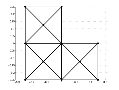
Figure 1: L-shaped domain as well as initial triangulation $\mathcal{T}_{0}$ with $\#\mathcal{T}_{0}=12$ triangles and initial boundary mesh $\mathcal{E}_{0}^{\Gamma}$ with $\#\mathcal{E}_{0}^{\Gamma}=8$ boundary elements.

\psfrag{error}[c][c]{error contribution $\rm err_{\ell}^{\Omega}$}\psfrag{nE}[c][c]{number of elements~{}$N$}\psfrag{convgraphResidual}[c][c]{}\psfrag{errbmcadap}{\tiny BMC, adap.}\psfrag{errbmcunif}{\tiny BMC, unif.}\psfrag{errjnadap}{\tiny JN, adap.}\psfrag{errjnunif}{\tiny JN, unif.}\psfrag{errsymadap}{\tiny sym, adap.}\psfrag{errsymunif}{\tiny sym, unif.}\psfrag{OON12}[c][c][1][-25]{\tiny$\mathcal{O}(N^{-1/2})$}\psfrag{OON13}[c][c][1][-17]{\tiny$\mathcal{O}(N^{-1/3})$}\includegraphics[width=216.81pt]{lin_conv_rates_error}

Figure 2: Volume error $\rm err_{\ell}^{\Omega}$ versus number of elements $N$ for Laplace problem of Section 7.1.

\psfrag{error}[c][c]{estimator contribution $\zeta_{\ell}^{\Omega}$}\psfrag{nE}[c][c]{number of elements~{}$N$}\psfrag{convgraphResidual}[c][c]{}\psfrag{estbmcadap}{\tiny BMC, adap.}\psfrag{estbmcunif}{\tiny BMC, unif.}\psfrag{estjnadap}{\tiny JN, adap.}\psfrag{estjnunif}{\tiny JN, unif.}\psfrag{estsymadap}{\tiny sym, adap.}\psfrag{estsymunif}{\tiny sym, unif.}\psfrag{OON12}[c][c][1][-27]{\tiny$\mathcal{O}(N^{-1/2})$}\psfrag{OON13}[c][c][1][-17]{\tiny$\mathcal{O}(N^{-1/3})$}\includegraphics[width=216.81pt]{lin_conv_rates_est}

Figure 3: Volume error estimator $\zeta_{\ell}^{\Omega}$ versus number of elements $N$ for Laplace problem of Section 7.1.

\psfrag{error}[c][c]{efficiency index $\zeta_{\ell}^{\Omega}/\rm err_{\ell}^{\Omega}$}\psfrag{nE}[c][c]{number of elements~{}$N$}\psfrag{convgraphResidual}[c][c]{}\psfrag{quotbmcadap}{\tiny BMC, adap.}\psfrag{quotbmcunif}{\tiny BMC, unif.}\psfrag{quotjnadap}{\tiny JN, adap.}\psfrag{quotjnunif}{\tiny JN, unif.}\psfrag{quotsymadap}{\tiny sym, adap.}\psfrag{quotsymunif}{\tiny sym, unif.}\includegraphics[width=216.81pt]{lin_quotients}

Figure 4: Efficiency index $\zeta_{\ell}^{\Omega}/\rm err_{\ell}^{\Omega}$ versus number of elements $N$ for Laplace problem of Section 7.1. The $x$-axis is scaled logarithmically.

\psfrag{error}[c][c]{error contribution $\rm err_{\ell}^{\Omega}$}\psfrag{tinsec}[c][c]{time $t$ [sec.]}\psfrag{compTime}[c][c]{}\psfrag{errbmcadap}{\tiny BMC, adap.}\psfrag{errbmcunif}{\tiny BMC, unif.}\psfrag{errjnadap}{\tiny JN, adap.}\psfrag{errjnunif}{\tiny JN, unif. }\psfrag{errsymadap}{\tiny sym, adap.}\psfrag{errsymunif}{\tiny sym, unif. }\includegraphics[width=216.81pt]{lin_comptime}

Figure 5: Comparison of the error versus the computing time for adaptive and uniform refinement strategy for Laplace problem of Section 7.1.

7.1 Laplace transmission problem on L-shaped domain

In this experiment, we consider the linear operator $\mathfrak{A}=\operatorname{Id}$. We prescribe the exact solution of (1) as

$$u(x,y) =r^{2/3}\sin(\tfrac{2}{3}\varphi),$$ (96)

$$u^{\rm ext}(x,y) =\tfrac{1}{2}\log(|x+\tfrac{1}{8}|^{2}+|y+\tfrac{1}{8}|^{2})$$ (97)

on an L-shaped domain, visualized in Figure 1. Here, $(r,\varphi)$ denote polar coordinates. These functions are then used to determine the data $(f,u_{0},\phi_{0})$. Note that $\Delta u=0=\Delta u^{\rm ext}$. We stress that $u$ has a generic singularity at the reentrant corner. Therefore, uniform mesh-refinement leads to a suboptimal convergence order $\alpha=1/3$. However, adaptive mesh-refinement recovers the optimal convergence rate $\alpha=1/2$. In Figure 2 resp. 3, we observe optimal rates for all error and error estimator quantities of the different coupling methods corresponding to the adaptive scheme, whereas all quantities corresponding to uniform mesh-refinement converge with order $\alpha=1/3$.

The quotients $\zeta_{\ell}^{\Omega}/\rm err_{\ell}^{\Omega}$, plotted in Figure 4, indicate that the residual-based estimators of Theorem 12, 16 and 21 are not only reliable but also efficient: We see that $\zeta_{\ell}^{\Omega}/\rm err_{\ell}^{\Omega}$ is constant for sufficiently large $N$.

When we compare the computing time, see Figure 5, we observe that the adaptive strategy is superior to the uniform one. Moreover, we see differences between the adaptive versions of the three coupling methods. The Bielak-MacCamy coupling needs significantly more computing time than the other coupling schemes. We also observe that the Johnson-Nédélec coupling is the fastest of all coupling methods, at least in this experiment.

7.2 Linear transmission problem on L-shaped domain

We consider a linear problem with $\mathfrak{A}=(c_{\rm ell}\tfrac{\partial u}{\partial x},\tfrac{\partial u}{\partial y})$ on an L-shaped domain. We again prescribe the solutions $(u,u^{\rm ext})$ by (96)–(97). Then, $\operatorname{div}\mathfrak{A}\nabla u=(c_{\rm ell}-1)\tfrac{\partial^{2}u}{\partial x^{2}}$. In Figure 6, we plot the error quantities $\rm err_{\ell}^{\Omega}$ of the adaptive schemes for different values of $c_{\rm ell}$. We observe good performance of both the Bielak-MacCamy and Johnson-Nédélec coupling also for $c_{\rm ell}\in(0,1/4]$, which was excluded by our analysis.

\psfrag{error}[c][c]{error contribution $\rm err_{\ell}^{\Omega}$, adaptive}\psfrag{nE}[c][c]{number of elements~{}$N$}\psfrag{ellipticity}[c][c]{}\psfrag{errbmc001}{\tiny BMC, $c_{\rm ell}=0.001$}\psfrag{errbmc25}{\tiny BMC, $c_{\rm ell}=0.25$}\psfrag{errjn001}{\tiny JN, $c_{\rm ell}=0.001$}\psfrag{errjn25}{\tiny JN, $c_{\rm ell}=0.25$}\psfrag{errsym001}{\tiny sym, $c_{\rm ell}=0.001$}\psfrag{errsym25}{\tiny sym, $c_{\rm ell}=0.25$}\psfrag{OON12}[l][B][1][-20]{\tiny$\mathcal{O}(N^{-1/2})$}\includegraphics[width=216.81pt]{gammaTest}

Figure 6: Convergence of the volume errors for different values of the ellipticity constant of the operator $\mathfrak{A}$ of Section 7.2 and adaptive mesh-refinement.

\psfrag{error}[c][c]{error contribution $\rm err_{\ell}^{\Omega}$, uniform}\psfrag{nE}[c][c]{number of elements~{}$N$}\psfrag{ellipticity}[c][c]{}\psfrag{errbmc001}{\tiny BMC, $c_{\rm ell}=0.001$}\psfrag{errbmc25}{\tiny BMC, $c_{\rm ell}=0.25$}\psfrag{errjn001}{\tiny JN, $c_{\rm ell}=0.001$}\psfrag{errjn25}{\tiny JN, $c_{\rm ell}=0.25$}\psfrag{errsym001}{\tiny sym, $c_{\rm ell}=0.001$}\psfrag{errsym25}{\tiny sym, $c_{\rm ell}=0.25$}\psfrag{OON13}[l][B][1][-19]{\tiny$\mathcal{O}(N^{-1/3})$}\includegraphics[width=216.81pt]{gammaTestUnif}

Figure 7: Convergence of the volume errors for different values of the ellipticity constant of the operator $\mathfrak{A}$ of Section 7.2 and uniform mesh-refinement.

7.3 Linear transmission problem with unknown solution

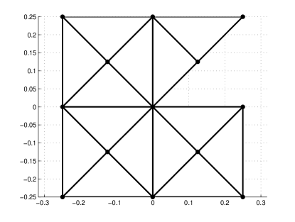
Figure 8: Z-shaped domain as well as initial triangulation $\mathcal{T}_{0}$ with $\#\mathcal{T}_{0}=14$ triangles and initial boundary mesh $\mathcal{E}_{0}^{\Gamma}$ with $\#\mathcal{E}_{0}^{\Gamma}=10$ boundary elements.

We present another experiment to underline the results of the aforegoing subsection. Again, we consider the operator $\mathfrak{A}$ with $\mathfrak{A}\nabla u=(c_{\rm ell}\tfrac{\partial u}{\partial x},\tfrac{\partial u}{\partial y})$, but now on a Z-shaped domain, visualized in Figure 8. The data is set to $(f,u_{0},\phi_{0})=(1,0,0)$, and we stress that the exact solution is not known. Therefore, we plot only the error estimator quantities $\zeta_{\ell}$ in Figure 9 resp. 10. An optimal convergence order $\alpha=1/2$ for the estimators corresponding to the adaptive schemes is observed, whereas uniform refinement methods lead to suboptimal convergence rates. As in Section 7.2, Figure 9 resp. 10 indicates a good performance of both the Johnson-Nédélec and Bielak-MacCamy coupling for $c_{\rm ell}\in(0,1/4]$.

\psfrag{error}[c][c]{error estimator $\zeta_{\ell}$, adaptive}\psfrag{nE}[c][c]{number of elements~{}$N$}\psfrag{ellipticity}[c][c]{}\psfrag{errbmc001}{\tiny BMC, $c_{\rm ell}=0.001$}\psfrag{errbmc25}{\tiny BMC, $c_{\rm ell}=0.25$}\psfrag{errjn001}{\tiny JN, $c_{\rm ell}=0.001$}\psfrag{errjn25}{\tiny JN, $c_{\rm ell}=0.25$}\psfrag{errsym001}{\tiny sym, $c_{\rm ell}=0.001$}\psfrag{errsym25}{\tiny sym, $c_{\rm ell}=0.25$}\psfrag{OON12}[l][B][1][-27]{\tiny$\mathcal{O}(N^{-1/2})$}\includegraphics[width=216.81pt]{gammaTest2}

Figure 9: Convergence of the respective error estimators $\zeta_{\ell}$ for different values of the ellipticity constant of the operator $\mathfrak{A}$ of Section 7.3 and adaptive mesh-refinement.

\psfrag{error}[c][c]{error estimator $\zeta_{\ell}$, uniform}\psfrag{nE}[c][c]{number of elements~{}$N$}\psfrag{ellipticity}[c][c]{}\psfrag{errbmc001}{\tiny BMC, $c_{\rm ell}=0.001$}\psfrag{errbmc25}{\tiny BMC, $c_{\rm ell}=0.25$}\psfrag{errjn001}{\tiny JN, $c_{\rm ell}=0.001$}\psfrag{errjn25}{\tiny JN, $c_{\rm ell}=0.25$}\psfrag{errsym001}{\tiny sym, $c_{\rm ell}=0.001$}\psfrag{errsym25}{\tiny sym, $c_{\rm ell}=0.25$}\psfrag{OON12}[l][B][1][-22]{\tiny$\mathcal{O}(N^{-1/2})$}\psfrag{OON13}[l][B][1][-15]{\tiny$\mathcal{O}(N^{-1/3})$}\includegraphics[width=216.81pt]{gammaTest2Unif}

Figure 10: Convergence of the respective error estimators $\zeta_{\ell}$ for different values of the ellipticity constant of the operator $\mathfrak{A}$ of Section 7.3 and uniform mesh-refinement.

7.4 Nonlinear experiment on Z-shaped domain

In the last experiment we consider a Z-shaped domain, visualized in Figure 8, and a nonlinear operator $\mathfrak{A}$ with $\mathfrak{A}\nabla u=g(|\nabla u|)\nabla u$, where $g(t)=2+1/(1+t)$ for $t\geq 0$. Note that the ellipticity constant of $\mathfrak{A}$ is $c_{\rm ell}=2$. The prescribed solution

$$u(x,y) =r^{4/7}\sin(\tfrac{4}{7}\varphi),$$ (98)

$$u^{\rm ext}(x,y) =\tfrac{x+y+0.25}{(x+0.125)^{2}+(y+0.125)^{2}}$$ (99)

of (1) fulfills $\Delta u^{\rm ext}=0$. The interior solution $u$ has a generic singularity at the reentrant corner. As can be seen in Figure 11, resp. 12, the uniform strategy leads to a suboptimal convergence rate $\alpha=2/7$, whereas the adaptive strategy leads to the optimal convergence rate $\alpha=1/2$.

\psfrag{error}[c][c]{error contribution $\rm err_{\ell}^{\Omega}$}\psfrag{nE}[c][c]{number of elements $N$}\psfrag{convgraphResidual}[c][c]{}\psfrag{errbmcadap}{\tiny BMC, adap.}\psfrag{errbmcunif}{\tiny BMC, unif.}\psfrag{errjnadap}{\tiny JN, adap.}\psfrag{errjnunif}{\tiny JN, unif.}\psfrag{errsymadap}{\tiny sym, adap.}\psfrag{errsymunif}{\tiny sym, unif.}\psfrag{OON12}[c][c][1][-27]{\tiny$\mathcal{O}(N^{-1/2})$}\psfrag{OON27}[c][c][1][-15]{\tiny$\mathcal{O}(N^{-2/7})$}\includegraphics[width=216.81pt]{nonlin_conv_rates_error}

Figure 11: Convergence of the volume error $\rm err_{\ell}^{\Omega}$ for the nonlinear experiment of Section 7.4.

\psfrag{error}[c][c]{estimator contribution $\zeta_{\ell}^{\Omega}$}\psfrag{nE}[c][c]{number of elements $N$}\psfrag{convgraphResidual}[c][c]{}\psfrag{estbmcadap}{\tiny BMC, adap.}\psfrag{estbmcunif}{\tiny BMC, unif.}\psfrag{estjnadap}{\tiny JN, adap.}\psfrag{estjnunif}{\tiny JN, unif.}\psfrag{estsymadap}{\tiny sym, adap.}\psfrag{estsymunif}{\tiny sym, unif.}\psfrag{OON12}[c][c][1][-27]{\tiny$\mathcal{O}(N^{-1/2})$}\psfrag{OON27}[c][c][1][-15]{\tiny$\mathcal{O}(N^{-2/7})$}\includegraphics[width=216.81pt]{nonlin_conv_rates_est}

Figure 12: Convergence of the volume error estimator quantities $\zeta_{\ell}^{\Omega}$ for the nonlinear experiment of Section 7.4.

\psfrag{error}[c][c]{efficiency index $\zeta_{\ell}^{\Omega}/\rm err_{\ell}^{\Omega}$}\psfrag{nE}[c][c]{number of elements $N$}\psfrag{convgraphResidual}[c][c]{}\psfrag{quotbmcadap}{\tiny BMC, adap.}\psfrag{quotbmcunif}{\tiny BMC, unif.}\psfrag{quotjnadap}{\tiny JN, adap.}\psfrag{quotjnunif}{\tiny JN, unif.}\psfrag{quotsymadap}{\tiny sym, adap.}\psfrag{quotsymunif}{\tiny sym, unif.}\includegraphics[width=216.81pt]{nonlin_quotients}

Figure 13: Efficiency index $\zeta_{\ell}^{\Omega}/\rm err_{\ell}^{\Omega}$ versus number of elements $N$ for the nonlinear experiment of Section 7.4. The $x$-axis is scaled logarithmically.

\psfrag{error}[c][c]{error}\psfrag{tinsec}[c][c]{time $t$ [sec.]}\psfrag{compTime}[c][c]{}\psfrag{error}[c][c]{error contribution $\rm err_{\ell}^{\Omega}$}\psfrag{compTime}[c][c]{}\psfrag{errbmcadap}{\tiny BMC, adap.}\psfrag{errbmcunif}{\tiny BMC, unif.}\psfrag{errjnadap}{\tiny JN, adap.}\psfrag{errjnunif}{\tiny JN, unif. }\psfrag{errsymadap}{\tiny sym, adap.}\psfrag{errsymunif}{\tiny sym, unif. }\includegraphics[width=216.81pt]{nonlin_comptime}

Figure 14: Comparison of the volume error versus the computing time for the nonlinear experiment of Section 7.4 and uniform resp. adaptive mesh-refinement.

The results of Figure 13 argue for the efficiency of the reliable error estimator $\zeta_{\ell}\in\{\rho_{\ell},\eta_{\ell},\zeta_{\ell}\}$, which matches our observations of the first experiment. As in Section 7.1, we obtain from Figure 14 that the adaptive strategy is superior to the uniform one.

7.5 Conclusion

In all our experiments, we observe that the adaptive mesh-refinement strategy empirically leads to optimal convergence rates for the error as well as for the error estimator quantities, whereas uniform refinement is inferior to the adaptive ones. Moreover, we see that the error quantities for the three different coupling methods differ only slightly. From this point of view, one cannot favour a certain coupling method. But we stress that there are significant differences in the computing times, where the Johnson-Nédélec coupling is superior to the other two coupling methods. Although the Bielak-MacCamy coupling is just the transposed problem of the Johnson-Nédélec coupling in the linear case, it needs the most computing time of all three coupling schemes. Furthermore, we have numerical evidence that the reliable error estimators corresponding to the different coupling schemes are also efficient.

Finally, we remark that our numerical experiments have shown that the assumption $c_{\rm ell}>1/4$ from Theorem 8 and 14 is sufficient for the solvability of the Bielak-MacCamy coupling and Johnson-Nédélec coupling, but not necessary.

- [1] M. Ainsworth, J.T. Oden: A posteriori error estimation in finite element analysis, Wiley-Interscience [John Wiley & Sons], New-York, 2000.
- [2] M. Aurada, M. Ebner, M. Feischl, S. Ferraz-Leite, P. Goldenits, M. Karkulik, M. Mayr, D. Praetorius: HILBERT — A Matlab implementation of adaptive 2D-BEM, ASC Report 24/2011, Institute for Analysis and Scientific Computing, Vienna University of Technology, Wien, 2011, software download at http://www.asc.tuwien.ac.at/abem/hilbert/
- [3] M. Aurada, S. Ferraz-Leite, D. Praetorius: Estimator reduction and convergence of adaptive BEM, Appl. Numer. Math., available online, 2011.
- [4] M. Aurada, M. Feischl, T. Führer, M. Karkulik, J.M. Melenk, D. Praetorius: Inverse estimates for elliptic integral operators and application to the adaptive coupling of FEM and BEM, preprint, 2012.
- [5] M. Aurada, M. Feischl, M. Karkulik, D. Praetorius: A posteriori error estimates for the Johnson-Nédélec FEM-BEM coupling, Eng. Anal. Bound. Elem. 36 (2012), 255–266.
- [6] M. Aurada, M. Feischl, D. Praetorius: Convergence of Some Adaptive FEM-BEM Coupling for elliptic but possibly nonlinear interface problems, Math. Model. Numer. Anal., accepted for publication (2011).
- [7] M. Aurada, M. Karkulik, D. Praetorius: Simple error estimates for hypersingular integral equations in adaptive 3D-BEM, In progress. (2012)
- [8] J. Bielak, R.C. MacCamy: An exterior interface problem in two-dimensional elastodynamics, Quart. Appl. Math. 41 (1983/84), 143–159.
- [9] C. Carstensen, A posteriori error estimate for the symmetric coupling of finite elements and boundary elements, Computing 57 (1996), 301–322.
- [10] C. Carstensen, S.A. Funken, E.P. Stephan, On the adaptive coupling of FEM and BEM in 2-d-elasticity, Numer. Math. 77 (1997), 187–221.
- [11] C. Carstensen, M. Maischak, E.P. Stephan: A posteriori error estimate and h-adaptive algorithm on surfaces for Symm’s integral equation, Numer. Math. (2001) 90, 197–213
- [12] C. Carstensen, E. Stephan: Adaptive coupling of boundary elements and finite elements, Math. Model. Numer. Anal. 29 (1995), 779–817.
- [13] M. Costabel: A symmetric method for the coupling of finite elements and boundary elements, in: The Mathematics of Finite Elements and Applications IV, MAFELAP 1987, (J. Whiteman ed.), Academic Press, London, 1988, 281–288.
- [14] M. Costabel, V.J. Ervin, E.P. Stephan: Experimental convergence rates for various couplings of boundary and finite elements, Math. Comput. Modelling 15 (1991), 93–102.
- [15] M. Feischl, M. Karkulik, J.M. Melenk, D. Praetorius: Quasi-optimal convergence rate for an adaptive boundary element method, ASC Report 28/2011, Institute for Analysis and Scientific Computing, Vienna University of Technology, Wien, 2011.
- [16] G. Gatica, G. Hsiao, F. Sayas: Relaxing the hypotheses of Bielak-MacCamy’s BEM-FEM coupling, preprint, 2009.
- [17] I. Graham, W. Hackbusch, S. Sauter: Finite elements on degenerate meshes: Inverse-type inequalities and applications, IMA J. Numer. Anal. 25 (2005), 379–407.
- [18] G. Hsiao, W. Wendland: Boundary integral equations, Applied Mathematical Sciences 164, Springer-Verlag, Berlin, 2008.
- [19] C. Johnson, J.C. Nédélec: On the coupling of boundary integral and finite element methods, Math. Comp. 35 (1980), 1063–1079
- [20] F. Leydecker, M. Maischak, E.P. Stephan, M. Teltscher, Adaptive FE-BE coupling for an electromagnetic problem in - a residual error estimator, Math. Methods Appl. Sci. 33 (2010), 2162–2186.
- [21] W. McLean: Strongly elliptic systems and boundary integral equations, Cambridge University Press, Cambridge, 2000.
- [22] S. Sauter, C. Schwab: Randelementmethoden: Analyse, Numerik und Implementierung schneller Algorithmen, Teubner Verlag, Wiesbaden, 2004.
- [23] F.J. Sayas: The validity of Johnson-Nédélec’s BEM-FEM coupling on polygonal interfaces, SIAM J. Numer. Anal. 47 (2009), 3451–3463.
- [24] L.R. Scott, S. Zhang: Finite element interpolation of nonsmooth functions satisfying boundary conditions, Math. Comp., 54 (1990), 483–493.
- [25] O. Steinbach: Numerical approximation methods for elliptic boundary value problems: Finite and boundary elements, Springer, New York, 2008.
- [26] O. Steinbach: A note on the stable one-quation coupling of finite and boundary elements, SIAM J. Numer. Anal. 49 (2011), 1521–1531.
- [27] E.P. Stephan, M. Maischak, A posteriori error estimates for fem-bem couplings of three-dimensional electromagnetic problems, Methods Appl. Mech. Engrg. 1994 (2005), 441–452.
- [28] R. Stevenson: The completion of locally refined simplicial partitions created by bisection, Math. Comp. 77 (2008), 227–241.
- [29] E. Zeidler: Nonlinear functional analysis and its applications, part II/B, Springer, New York, 1990.