DØ INTERNAL DOCUMENT – NOT FOR PUBLIC DISTRIBUTION

Validity of Transport Energy in Disordered Organic Semiconductors

Abstract

A systematic study of the transport energy in disordered organic semiconductors based on variable range hopping theory has been presented here. The temperature, electric field, material disorder and carrier concentration dependent transport energy is extensively discussed. We demonstrate here, transport energy is not a general concept and invalid even in low electric field and concentration regime.

Understanding the charge transport mechanism in disordered organic semiconductors such as conjugated and molecularly doped polymers, is of crucial importance to design and synthesize better materials. Physical transport phenomena in organic semiconductors are in general very complex and arise from energy and spatial disorder, which invalidates the use of the traditional band transport theories based on the periodic distribution of atoms in inorganic crystals. Currently, charge transport in organic semiconductors is often described in terms of hopping theory mott . A fundamental work in the modeling of the hopping transport in organic semiconductors is the Gaussian disorder model proposed by Bassler bassler1 ; bassler2 . Subsequent to this Monte Carlo simulation, a number of theoretical investigations concerning charge transport in amorphous organic systems utilizing the Gaussian approach have been published and considerable progress in the analytical description of the problem has been made novikov ; dunlap ; arkhipov1 ; li1 . An important simplification of the complex hopping transport mechanism was the introduction of the transport energy concept, This concept allows the complex hopping mechanism in the band tails to be interpreted in terms of a multiple-trapping-and-release model, where the transport energy plays the role similar to the mobility edge in amorphous inorganic semiconductors monro ; arkhipov2 ; li2 ; baranovskii1 ; baranovskii2 ; roland1 . Thermally stimulated luminescencebassler3 , carrier dependent mobilityblom1 ; baranovskii3 ; li2 ; vissenberg , seebeck coefficient germs , as well as injection phenomenaarkhipov3 , have already been described utilizing this transport energy concept. Despite the concept of transport energy has widely been applied to describe the charge hopping transport of different organic semiconductors, the validity of this concept is nontrivial. As transport energy is derived on the basis of zero electric field and low carrier concentration regime, and only the hopping upwards transport is concerned. However, in the real disordered organic semiconductors devices, the electric field could reach $1\times 10^{8}V/m$ and carrier concentration could as high as $1\times 10^{26}m^{-3}$,therefore, the applicability of the transport energy to real disordered organic semiconductors should be a matter of intensive research, where it is important to distinguish whether the organic semiconductor exist the mobility edge (transport energy) or whether this concept could be used to describe the mobility in hopping system. In this letter, we show how the transport energy changes with temperature, electric field, carrier concentration and material disorder. Using this analysis, we conclude that the transport energy is not a general concept and invalid in real disordered organic semiconductors.

Model.—Generally speaking, there are two ways to define he concept of transport energy in organic semiconductors, both of them are based on the Miller-Abrahams expressions miller , the hopping transport takes place via tunneling between an initial states $i$and a target states$j$.The tunneling process is described as

$$\nu=\nu_{0}\exp\left(-u\right)=\nu_{0}\left\{\begin{array}[]{c}\exp\left(-2\alpha R_{ij}-\frac{E_{j}-E_{i}}{kT}\right),E_{i}>E_{j}\\ \left(-2\alpha R_{ij}\right).\qquad\qquad\qquad E_{i}<E_{j}\\ \end{array}\right.$$ (1)

Here, $\nu_{0}$ is the attempt-to-jump frequenct, $R_{ij}$ is the hopping distance, $u$ is the hopping range arkhipov2 ,$E_{i}$ and $E_{j}$ are the eneries at site $i$ and $j$, respectively, $\alpha$ is the inverse localized length and $k$ is the Boltzmann constant. Then, if only the hopping upwards $\nu_{\uparrow}$ is taken into account, the transport energy is defined as the finial energy $E_{t}$ that the hopping transport has maximum rate, so $E_{t}$ could be obtained by the equation as baranovskii2

$$\frac{\partial\nu_{\uparrow}}{\partial E_{t}}=0.$$ (2)

This gives

$$g\left(E_{t}\right)\left[\int^{E_{t}}_{-\infty}g\left(E\right)dE\right]^{-4/3}=\frac{1}{\alpha kT}\left(\frac{9\pi}{2}\right)^{1/3}.$$ (3)

Where $g\left(E\right)$ is the density of states (DOS). Here we can see that the hopping transport is limited by upward transitions from filled states to empty states and the transport energy has been defined as the preferred energy to which the fastest upward transitions occur.
In the other case, the transport energy is derived based on the average number of target sites $n\left(E_{i},u\right)$ as

$$n\left(E_{i},u\right)=\int_{0}^{u/{2\alpha}}R_{ij}^{2}dR_{ij}\int_{-\infty}^{E_{i}+kT\left(u-2\alpha\right)}g\left(E\right)dE.$$ (4)

If we disregard the hopping downwards and choose the starting energy $E_{i}$ as $-\infty$, the transport energy could be obtained by setting $n\left(E_{i},u\right)=1$ and the result is arkhipov2

$$\int_{-\infty}^{E_{t}}g\left(E\right)\left(E_{t}-E\right)^{3}dE=\frac{6}{\pi}\left(\alpha kT\right)^{3}.$$ (5)

This definition hints that the transport energy is the site energy to which the hopping upwards need the least energy in energy space.
When there exists an electric field $F$, the electric field will lower the Coulomb barrier, which leads to the reduction of the thermal activation energies, and the hopping range with normalized energy can therefore be rewritten as apsley ; li3

$$u=\left\{\begin{array}[]{c}2\alpha\left(1+\beta\right)R_{ij}+\epsilon_{j}-\epsilon_{i},\epsilon_{j}>\epsilon_{i}-\beta\cos\theta\\ \left(2\alpha R_{ij}\right).\qquad\qquad\qquad\epsilon_{j}<\epsilon_{i}-\beta\cos\theta\\ \end{array}\right.$$ (6)

Where $\beta=Fe/{2\alpha kT}$ and and $\theta$ is the angle between $R_{ij}$ and the electric field ranging from $0$ to $pi$.For a site with energy $\epsilon_{i}$ in the hopping space, the most probable hop for a carrier on this site is to an empty site at a range $u$, where it needs the minimum energy. Conduction is the result of a long sequence of hops through this hopping space. Then, following the method in apsley , we derive the number of empty sites enclosed by the constant range $u$, as

$$n\left(\epsilon_{i},u,F\right)=\qquad\qquad\qquad\qquad\qquad\qquad\qquad\qquad\qquad$$

$$\frac{1}{8\alpha^{3}}\int_{0}^{\Pi}d\theta\sin\theta\int_{0}^{u}dr2\pi r^{2}\int_{-\infty}^{u+\epsilon_{i}-r\left(1+\beta\cos\theta\right)}d\epsilon$$

$$\times g\left(\epsilon\right)\left[1-f\left(\epsilon,\epsilon_{F}\right)\right].$$ (7)

Here $f\left(\epsilon,\epsilon_{F}\right)$ is the Fermi Dirac distribution and $1-f\left(\epsilon,\epsilon_{F}\right)$ is the probability that the finial site is empty, the Fermi energy $\epsilon_{F}$ is calculated by the condition

$$c=\int_{-\infty}^{\infty}d\epsilon\frac{g\left(\epsilon\right)}{1+exp\left(\epsilon-\epsilon_{F}\right)}.$$ (8)

Here $c$ is the carrier concentration. By change the integration variable, equation (7) will be in the form of

$$n\left(\epsilon,u,F\right)=\frac{2\pi}{3\times 8\alpha^{3}}\int_{-1}^{1}d\tau\qquad\qquad\qquad\qquad$$

$$\times\left[\int_{\epsilon_{i}-\beta u\tau}^{\epsilon_{i}+u}d\epsilon g\left(\epsilon\right)\frac{\left(u+\epsilon_{i}-\epsilon\right)^{3}}{\left(1+\beta\tau\right)^{3}}+\int_{-\infty}^{\epsilon_{i}-\beta u\tau}d\epsilon g\left(\epsilon\right)\right]$$ (9)

The first term on the right-hand side of equation (9) gives the number of shallower states,and the second one describes the number of target states which are deeper than the starting site . According to the variable range hopping theory apsley ; arkhipov1 ; baranovskii3 , at a given field and temperature, almost every starting localized state has only one well distinguished nearest empty target hopping neighbor, i.e. another localized state that is characterized by the minimum value of the hopping range, this range could be obtained by solving the equation

$$n\left(\epsilon_{i},F,u\right)=1.$$ (10)

This equation established the basis of our model. the target site energy for every hopping process can be well evaluated from the euqation (10).

Validity of Arkhipov transport energy.—To check this model validity, we disregard the downwards hopping as well, equation (9) then reads as

$$1=\frac{2\pi}{3\times 8\alpha^{3}}\int_{-1}^{1}d\tau\int_{\epsilon_{i}-\beta u\tau}^{\epsilon_{i}+u}d\epsilon g\left(\epsilon\right)\frac{\left(u+\epsilon_{i}-\epsilon\right)^{3}}{\left(1+\beta\tau\right)^{3}}$$ (11)

Using the developed model equation (11), we now proceed to calculate the relation between starting energy and finial energy in real disordered organic semiconductors. We take the Gaussian form $g\left(\epsilon\right)=\frac{N_{t}}{\sqrt{2\pi}\sigma}\exp\left(-\frac{\epsilon^{2}}{2\sigma^{2}}\right)$ density of states in the full manuscript, where $N_{t}$ is the number of states per unit volume and $\sigma=\sigma_{0}/kT$ indicates the width of the DOS. $N_{t}=1\times 10^{28}m^{-3}$ is taken in the full manuscript, a typical value for the relevant organic semiconductors. It is instructive to calculate this target energy as a function of the initial energy for different carrier concentration, corresponding to different fermi-level, the results are displayed in the insert of Fig. 1. A clear observation is that, in this situation, the transport energy does exist for deeper starting energy but increases with the carrier concentration. Field dependent transport energy is plotted in the Fig.1, the same as concentration dependent transport energy, field does not change transport energy for deeper energies but decreases for field higher than $1\times 10^{7}V/m$, this field strength is actually low field for most organic devices. The reason for the decrease of transport energy is that, the electric field can change the energy difference between the finial and target sites, and thereby, assist carrier jumps along the field direction, so the target energy will decrease on the contrary. For the very low carrier concentration, the field and concentration dependent transport energy could be derived as

$$n\left(\epsilon,u,F\right)\approx\frac{2\pi}{24\alpha^{3}\left(1-\beta^{2}\right)^{2}}\int_{\epsilon_{i}-\beta u}^{\epsilon_{i}+u}g\left(\epsilon\right)\left(\epsilon_{i}+u-\epsilon\right)^{3}d\epsilon$$

$$=\frac{2\pi}{24\alpha^{3}\left(1-\beta^{2}\right)^{2}}\int_{-\infty}^{\epsilon_{t}}g\left(\epsilon\right)\left(\epsilon_{t}-\epsilon\right)^{3}d\epsilon\qquad\qquad$$ (12)

Certainly, this is not a general concept as well.
We then consider the effect of the lattice disorder, which is caused by the random molecular packing in organic semiconductors hulea . The relation between transport energy and materials disorder $\sigma$ is shown in Fig. 2 (a). An important result is that, the transport energy is invalid for higher energies, but these energies make sense for the charge transport in real organic semiconductors. It is well known, in the low carrier concentration regime, the hopping usually jumps from the so-called equilibrium energy $E_{\infty}=-\left(\sigma\right/kT)^{2}=-25kT$ for $\sigma/kT=5$; In the high carrier concentration regime, the carrier jumps from Fermi energy ($\epsilon_{F}=-20k_{B}T$ here). An obvious feature appears here is the transport energy does not exist for energy higher than $-18kT$ in the case of $\sigma/kT=5$. In organic semiconductors, $\sigma=5kT$ correspond to $\sigma=0.12ev$ at room temperature, a typical value for organic semiconductors blom3 . Therefore, the transport energy has no generality and is invalid for real organic semiconductor system. Please note that the field used here is $1\times 10^{5}V/m$, which is low field regime; the fermi energy chosen here is also corresponding to the low concentration regime. The other parameters values are also typical ones for organic semiconductors such as $\alpha=1nm$. To investigate the reason for this phenomena, we plot the ratio between downwards and upwards hopping in Fig. 2(b), one can see clearly that, the downwards hopping has little effect on the charge transport characteristics and should not account for this result. One possible explanation is, for the small disorder Gsussian DOS, since the carriers have few nearest neighbor sites to choose and it is reasonable to hop to the same energy; But for the wider Gaussian DOS, carriers has more near neighbor sites and more active, hence the target energy will be random according to the calculation. Therefore, the approximation in baranovskii2 ; arkhipov1 that the the transport energy in zero field is independent the starting energy is not correct in real organic semiconductors.

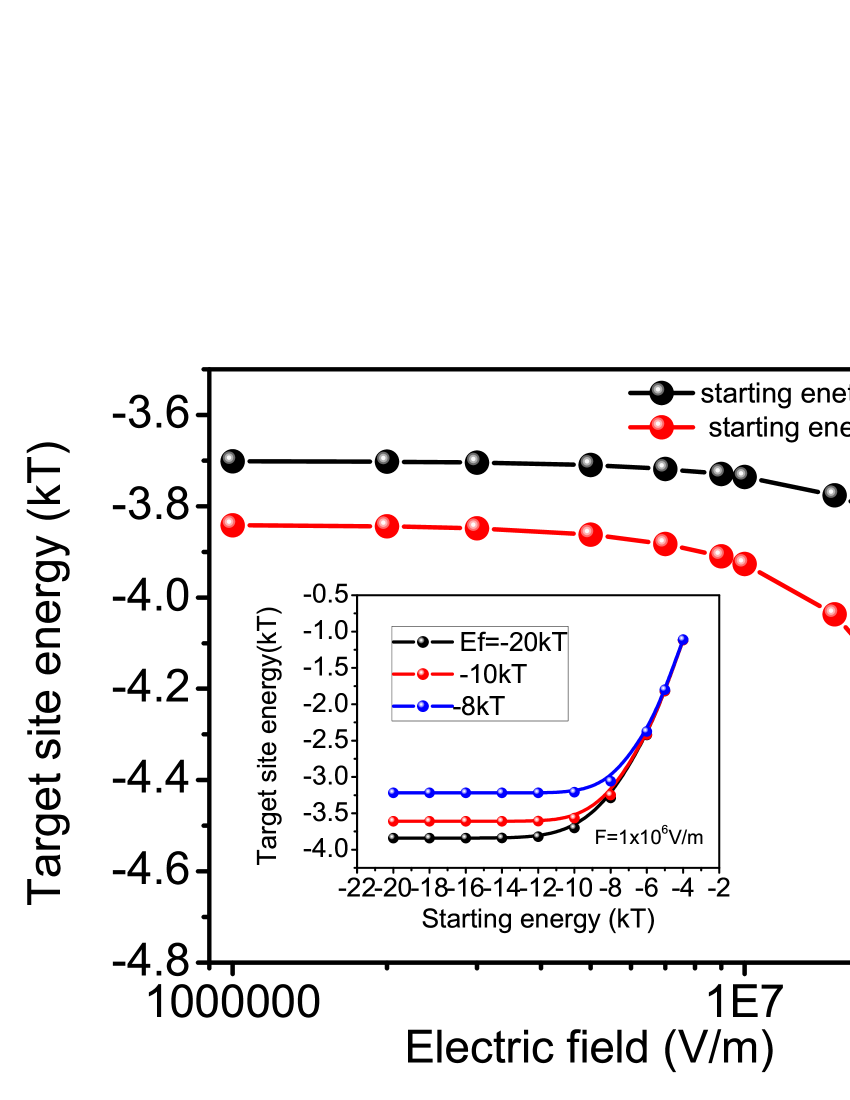
Figure 1: The computed transport energy as function of the starting energy for different electric field . The inset shows the carrier concentration (Fermi level) dependent transport energy.

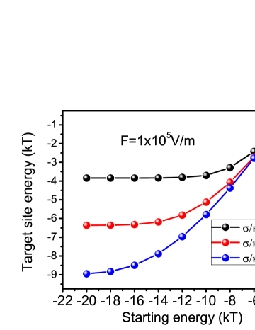
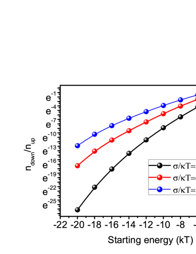
Figure 2: (a) The disorder dependent transport energy for different starting energy. (b) The ratio of hopping-downwards site number and hopping upwards number

The question arises now on how much difference between the calculated mobility using Akhipov method and the work here. The comparison is shown in Fig. 3. It is clearly seen that, in the low temperature regime, Akhipov model will underestimate the mobility but overestimate the mobility in high temperature. And this trend is even more pronounced with carrier concentration increasing.

Validity of Baranovskii transport energy model.—According to the definition of Baranovskii transport energy, the hopping upwards rate has maximum value for every jumping, hence, we derivative equation (6) as

$$\left\{\begin{array}[]{rl}\frac{\partial\nu_{\uparrow}}{\partial\epsilon_{j}}=2\alpha\left(1+\beta\right)\frac{\partial R_{ij}}{\partial\epsilon_{j}}+1=0,\\ \frac{\partial\nu_{\uparrow}}{\partial\theta}=2\alpha\left(1+\beta\right)\frac{\partial R_{ij}}{\partial\theta}=0,\\ 1=4\pi R_{ij}^{2}\int_{0}^{\theta}\sin\theta d\theta\int_{-\infty}^{\epsilon_{j}}d\epsilon g\left(\epsilon\right)\left[1-f\left(\epsilon,\epsilon_{F}\right)\right].\\ \end{array}\right.$$ (13)

The $R_{ij}$ that is the function of $\theta$ and $\epsilon_{j}$, could be obtained as the equation (11). Connecting Gaussian DOS and equation(12), we numerically calculate the transport energy for this definition. The concentration dependent transport energy is shown in Fig. 4. The deviation of target energy from the transport energy is more dramatic, even at the starting energy $\epsilon_{i}=24k_{B}T$, the transport energy is obvious invalid. This holds for the field dependent transport energy (the insert figure), too. We also find, the same conclusion is obtained by introducing the percolation parameter baranovskii2 in equation (13) .

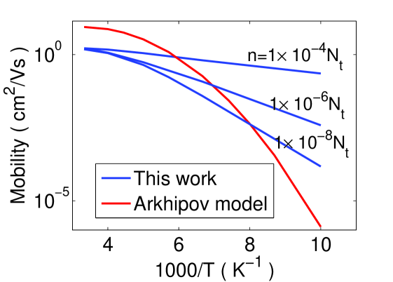
Figure 3: The Comparison between the calculated mobility in this work ($F=5\times 10^{4}V/cm$) and Akhipov mobility model for different temperatures.

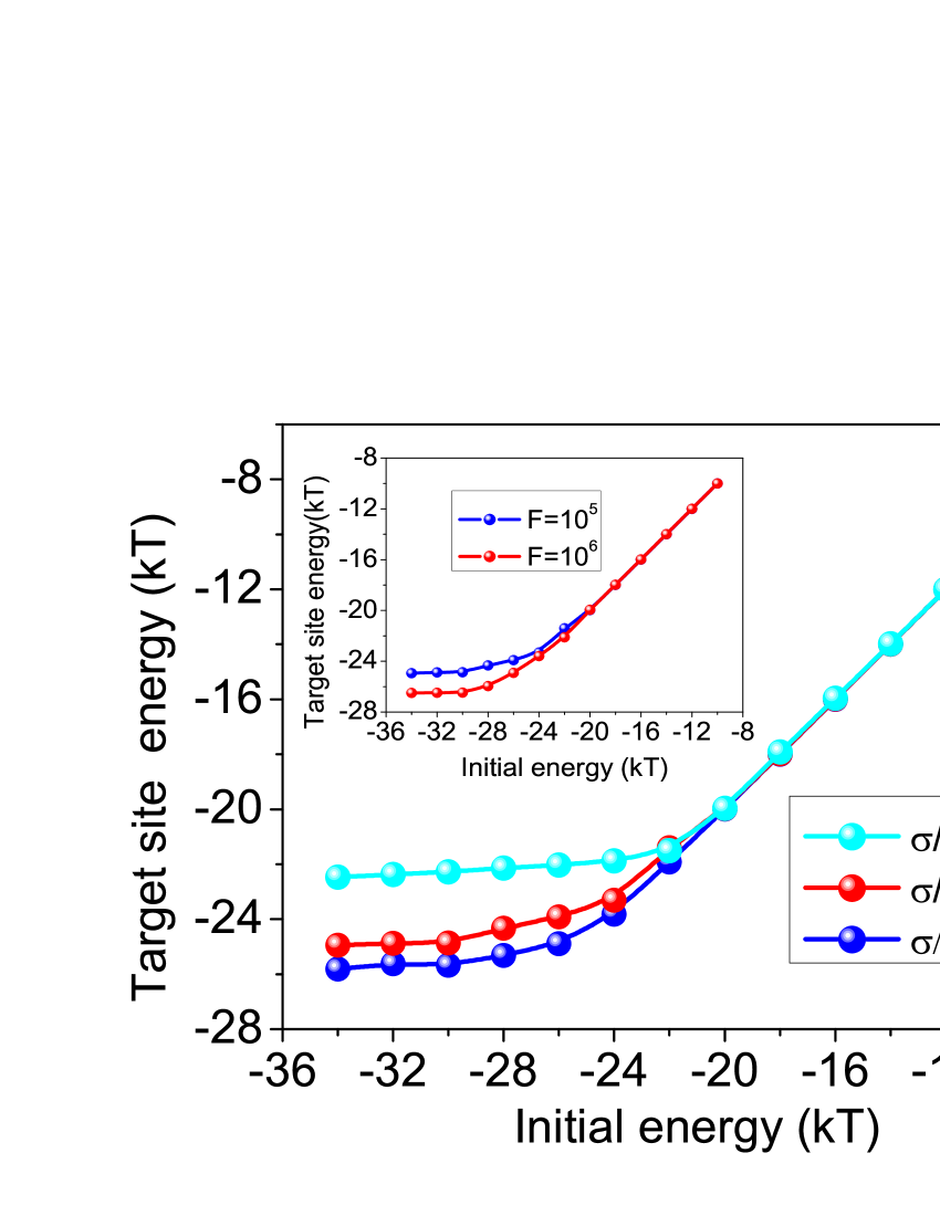
Figure 4: The computed Baranovskii transport energy as function of the starting energy for different electric field . The inset shows the electric field dependent Baranovskii transport energy.

In conclusion, the validity of the transport energy in disordered organic semiconductors has been investigated intensively. The results shows, neither Baranovskii nor Arkhipov definition for the transport energy is valid in real organic semiconductors system, even in the low field regime, the transport energy lost the universality. This issue was not adequately addressed for in earlier evaluations of the transport energy based on the hopping rates. Concomitantly, the use of the previously obtained expressions for transport energy in calculations of the carrier transport parameters would lead to incorrect results for the concentration dependencies of these parameters baranovskii4 ; li4 ; arkhipov4 ; germs . It should be mentioned that these calculations are describing only the first release step. These oscillating jumps of the released carriers may jump back to their initial state do not contribute effectively to the charge transport arkhipov2 . Finally, we mention that the description presented here should also be applicable to describe the temperature, electric field and carrier concentration dependent charge transport properties, for example mobility, as we have done in li3 .

Financial support from NSFC (No. 60825403) and National 973 Program 2011CB808404 is acknowledged.

References

- (1) N. F. Mott, J. Phys. C 20, 3075 (1987).
- (2) H. Bassler,Phys. Status Solidi B Res. A 175, 15 (1993).
- (3) H. Bassler,Phys. Status Solidi B Res. A 107, 9 (1981).
- (4) S. N. Novikov, D. H. Dunlap, V. M. Kenkre, P. E. Parris, and A. V. Vannikov, Rev. Lett. A 81, 4472 (1998).
- (5) D. H. Dunlap, V. M. Kenkre, P. E. Parris, and A. V. Vannikov, Rev. Lett. A 77, 542 (1996).
- (6) V. I. Arkhipov, E. V. Emelianova, and H. Bassler, Philos. Mag. B 81, 985 (2001).
- (7) L. Li, G. Meller, and H. Kosina, Appl. Phys. Letter. 98, 023305 (2011).
- (8) D. Monro, Phys. Rev. Lett. 54 146 (1985).
- (9) V. I. Arkhipov, E. V. Emelianova, and G. J. Adriaenssens, Phys. Rev. B 64, 985 (2001), 125125(2001).
- (10) L. Li, G. Meller, and H. Kosina, Appl. Phys. Lett.92 013307 (2008).
- (11) S. D. Baranovskii, H. Cordes, S. Yamasaki, and P. Thomas, Phys. Status. Solidi B 230, 281 (2002).
- (12) O. Rubel, S. D. Baranovskii, H. Cordes, P. Thomas, and S. Yamasaki, Phys. Rev. B 69, 014206 (2004).
- (13) R. Schmechel, J. Appl. Phys. 93, 4653 (2003).
- (14) A. Kadashchuk, Y. Skryshevskii, A. Vakhnin, N. Ostapenko, V. I. Arkhipov, E. V. Emelianova, and H. Bassler, Phys. Rev. B 63, 115205 (2001).
- (15) C. Tanase, E. G Meijer, P. W. M. Blom, and D. M. de Leeuw, Phys. Rev. Lett 91, 216601 (2003).
- (16) J. O. Oelerich, D. Huemmer, and S D. Baranovskii,Phys. Rev. Lett 108, 226403 (2012).
- (17) M. C. J. M Vissenberg, and M. Matters,Phys. Rev. B. 57, 12964 (1998).
- (18) W. Chr. Germs, K. Guo, R. A. J. Janssen, and M. Kemerink,Phys. Rev. Lett. 109, 016601 (2012).
- (19) V. I. Arkhipov, U. Wolf, and H. Bassler, Philos. Mag. B 59, 7514 (1999).
- (20) A. Miller, and E. Abraham, Phys. Rev. B 120, 745 (1960).
- (21) N. Apsley, and H. P. Hughes, Philos. Mag. 31, 1327 (1975).
- (22) L. Li, S. Winckel, J. Genoe, and P. Heremans, Appl. Phys. Lett.95 153301 (2009).
- (23) I N. Hulea, H. B. Brom, A .J. Houtepen, D. Vanmaekelbergh, J. J. Kelly, and E. A. Meuenkamp, Phys. Rev. Lett.93 166601 (2004).
- (24) W. F. Pasveer, J. Cottaar, C .Tamase, R. Coehoorn, P. A. Bobbert, P. W. M. Blom, D. M. de Leeuw, and M. A.J Michels, Phys. Rev. Lett.94 206601 (2005).
- (25) L. Li, G. Meller, and H. Kosina, J. Appl. Phys.106 013714 (2008).
- (26) V. I. Arkhipov, E. V. Emelianova, G. J. Adriaenssens and H. Bassler, J. Non-Crys. Solids 299, 1047 (2002).
- (27) R. Coehoorn, W. F. Pasveer, P. A. Bobbert, and M. A. J. Michels,Phys. Rev. B 72, 155206 (2005).