On the Pareto-Optimal Beam Structure and Design for Multi-User MIMO Interference Channels

Abstract

In this paper, the Pareto-optimal beam structure for multi-user multiple-input multiple-output (MIMO) interference channels is investigated and a necessary condition for any Pareto-optimal transmit signal covariance matrix is presented for the $K$-pair Gaussian $(N,M_{1},\cdots,M_{K})$ interference channel. It is shown that any Pareto-optimal transmit signal covariance matrix at a transmitter should have its column space contained in the union of the eigen-spaces of the channel matrices from the transmitter to all receivers. Based on this necessary condition, an efficient parameterization for the beam search space is proposed. The proposed parameterization is given by the product manifold of a Stiefel manifold and a subset of a hyperplane and enables us to construct a very efficient beam design algorithm by exploiting its rich geometrical structure and existing tools for optimization on Stiefel manifolds. Reduction in the beam search space dimension and computational complexity by the proposed parameterization and the proposed beam design approach is significant when the number of transmit antennas is larger than the sum of the numbers of receive antennas, as in upcoming cellular networks adopting massive MIMO technologies. Numerical results validate the proposed parameterization and the proposed cooperative beam design method based on the parameterization for MIMO interference channels.

I Introduction

Multi-user multiple antenna interference channels have gained intensive interest from research communities in recent years because of the significance of proper interference control in current and future wireless networks. One of the break-through results in this area is interference alignment by Cadambe and Jafar [1], which provides an effective way to achieving maximum degrees-of-freedom (DoF) for MIMO interference channels. However, interference alignment is only DoF optimal, i.e., it is optimal at high signal-to-noise ratio (SNR), whereas in typical cellular networks most receivers experiencing severe interference are located at cell edges and hence operate in the low or intermediate SNR regime. Thus, Jorswieck et al. investigated the multiple antenna interference channel problem from a different perspective based on Pareto-optimality [2]. The framework of Pareto-optimality is especially useful for interference channels since the users in an interference channel basically form a group for negotiation. Under this framework, Jorswieck et al. showed for multiple-input single-output (MISO) interference channels that any Pareto-optimal beam vector at a transmitter is a normalized convex combination of the zero-forcing (ZF) beam vector and the matched-filtering (MF) beam vector in the case of two users and a linear combination of the channel vectors from the transmitter to all receivers in the general case of an arbitrary number of users. Their result and subsequent results by other researchers provide useful parameterizations for the optimal beam search space for efficient cooperative beam design in MISO interference channels [3, 4, 5, 6, 7, 8]. However, not many results for the Pareto-optimal beam structure for MIMO interference channels are available, although there exist some results in limited circumstances [9, 10, 11].

In this paper, we provide a necessary condition for Pareto-optimal beamformers for the $K$-pair Gaussian $(N,M_{1},$ $\cdots,M_{K})$ interference channel, which can model general MIMO interference channels, and show that any Pareto-optimal transmit signal covariance matrix at a transmitter should have its column space contained in the union of the eigen-spaces of the channel matrices from the transmitter to all receivers. Based on this, we provide an efficient parameterization for the beam search space not missing Pareto-optimality whose dimension is independent of the number $N$ of transmit antennas and is determined only by $(M_{1},\cdots,M_{K})$, when $N\geq\sum_{i=1}^{K}M_{i}$. The proposed parameterization is given by the product manifold of a Stiefel manifold and a subset of a hyperplane and enables us to construct a very efficient cooperative beam design algorithm by exploiting its rich geometrical structure and existing tools for optimization on Stiefel manifolds. Reduction in the beam search space dimension and computational complexity by the proposed parameterization and the proposed beam design algorithm is significant, when $N>>\sum_{i=1}^{K}M_{i}$ as in upcoming cellular systems adopting massive MIMO technologies [12, 13]. Furthermore, the proposed beam design algorithm does not need to fix the number of data streams for transmission beforehand and it finds an (locally) optimal DoF for a given finite SNR. This is beneficial because the optimal DoF is not known for a finite SNR in most cases.

Notations and Organization    In this paper, we will make use of standard notational conventions. Vectors and matrices are written in boldface with matrices in capitals. All vectors are column vectors. For a matrix ${\bf A}$, ${\bf A}^{H}$, $\|{\bf A}\|$, $\mbox{tr}({\bf A})$, and $|{\bf A}|$ indicate the Hermitian transpose, 2-norm, trace, and determinant of ${\bf A}$, respectively. ${\bf A}_{ij}$ or $[{\bf A}]_{ij}$ denotes the element in the $i$-th row and the $j$-th column of ${\bf A}$. ${\cal C}({\bf A})$ denotes the column space of ${\bf A}$ and ${\cal C}^{\perp}({\bf A})$ denotes the orthogonal complement of ${\cal C}({\bf A})$. ${\bf P}_{{\cal L}}({\bf v})$ denotes the orthogonal projection of a vector ${\bf v}$ onto a linear subspace ${\cal L}$. ${\bf\Pi}_{{\bf A}}={\bf A}({\bf A}^{H}{\bf A})^{-1}{\bf A}^{H}$ represents the orthogonal projection onto ${\cal C}({\bf A})$ and ${\bf\Pi}_{{\bf A}}^{\perp}={\bf I}-{\bf\Pi}_{{\bf A}}$. For matrices ${\bf A}$ and ${\bf B}$, ${\bf A}\succcurlyeq{\bf B}$ means that ${\bf A}-{\bf B}$ is positive semi-definite. ${\bf I}_{n}$ stands for the identity matrix of size $n$ (the subscript is omitted when unnecessary). $[{\bf a}_{1},\cdots,{\bf a}_{L}]$ or $[{\bf a}_{i}]_{i=1}^{L}$ denotes the matrix composed of vectors ${\bf a}_{1},\cdots,{\bf a}_{L}$ and $\mbox{diag}(a_{1},\cdots,d_{n})$ denotes the diagonal matrix with elements $a_{1},\cdots,a_{n}$. ${\bf x}\sim\mathcal{CN}(\hbox{\boldmath$\mu$\unboldmath},\hbox{$\bf\Sigma$})$ means that ${\bf x}$ is circularly-symmetric complex Gaussian-distributed with mean vector $\mu$ and covariance matrix $\bf\Sigma$. ${\mathbb{R}}$, ${\mathbb{R}}_{+}$, and ${\mathbb{C}}$ denote the sets of real numbers, non-negative real numbers, and complex numbers, respectively. ${\mathbb{R}}^{n}$ denotes the $n$-dimensional Euclidean space and ${\mathbb{C}}^{n}$ denotes the vector space of all complex $n$-tuples. ${\mathbb{C}}^{n\times p}$ is the set of all $n\times p$ matrices with complex elements. For a complex number $a$, $\mbox{Re}\{a\}$ denotes the real part of $a$.

The remainder of this paper is organized as follows. The system model is described in Section II. In Section III, a necessary condition and a parameterization for Pareto-optimal transmit beamformers for MIMO interference channels are provided. In Section IV, a beam design algorithm under the obtained parameterization is presented. Numerical results are provided in Section V, followed by conclusions in Section VI.

II System Model

In this paper, we consider a Gaussian interference channel with $K$ transmitter-receiver pairs, where every transmitter has $N$ transmit antennas and receiver $i$ has $M_{i}$ receive antennas. We assume that $M_{i}\geq 1$, $i=1,\cdots,K$, and $N\geq\max\{M_{1},\cdots,M_{K}\}$. Due to interference from the unwanted transmitters, the received signal vector ${\bf y}_{i}$ at receiver $i$ is given by

$${\bf y}_{i}={\bf H}_{ii}{\bf s}_{i}+\sum_{j=1,j\neq i}^{K}{\bf H}_{ij}{\bf s}_{j}+{\bf n}_{i},$$ (1)

where ${\bf H}_{ij}$ denotes the $M_{i}\times N$ channel matrix from transmitter $j$ to receiver $i$; ${\bf s}_{j}$ is the $N\times 1$ transmit signal vector at transmitter $j$ generated from Gaussian distribution $\mathcal{CN}(0,{\bf Q}_{j})$; and ${\bf n}_{i}$ is the additive Gaussian noise vector at receiver $i$ with distribution ${\mathcal{CN}}(0,{\bf I})$. Here, the transmit signal covariance matrix ${\bf Q}_{j}~{}(={\mathbb{E}}\{{\bf s}_{j}{\bf s}_{j}^{H}\})$ at transmitter $j$ is chosen among the feasible set

$$\mathcal{Q}_{j}:=\{{\bf Q}\in\mathbb{C}^{N\times N}~{}:~{}{\bf Q}\succcurlyeq\mathbf{0},~{}\text{tr}({\bf Q})\leq P_{j},~{}\text{and}~{}1\leq\text{rank}({\bf Q})\leq M_{j}\},$$ (2)

where the rank constraint is imposed to guarantee that the number of transmitted data streams is at least one and is less than or equal to the possible maximum $M_{j}=\min\{M_{j},N\}$ for transmitter $j$, $j=1,\cdots,K$. Note that any value of degree-of-freedom (DoF) from one to the maximum $M_{j}$ is feasible within the feasible set ${\cal Q}_{j}$. From here on, we will call the considered MIMO interference channel the $K$-pair Gaussian $(N,M_{1},\cdots,M_{K})$ MIMO interference channel. The considered $K$-pair Gaussian $(N,M_{1},\cdots,M_{K})$ MIMO interference channel model is especially useful for downlink cooperative transmit beamforming in cellular systems. In the cellular downlink case, the transmitters, i.e., basestations can be equipped with many transmit antennas and the number of transmit antennas can be set to be the same in the phase of network design. On the other hand, each receiver, i.e., a mobile station has one or two receive antennas and furthermore the receivers forming a cooperative beamforming group together with the cooperating basestations may not have the same number of antennas. The $K$-pair $(N,M_{1},\cdots,M_{K})$ MIMO interference channel model fits this situation exactly.

Due to the assumption of $N\geq\max\{M_{i},i=1,\cdots,,K\}$, the $M_{i}\times N$ channel matrix ${\bf H}_{ij}$ is a fat matrix (i.e., the number of its columns is larger than or equal to that of its rows) and its singular value decomposition (SVD) is given by

$${\bf H}_{ij}={\bf U}_{ij}[\hbox{$\bf\Sigma$}_{ij},~{}\mathbf{0}][{\bf V}_{ij}^{\parallel},{\bf V}_{ij}^{\bot}]^{H},$$ (3)

where ${\bf U}_{ij}\in{\mathbb{C}}^{M_{i}\times M_{i}}$ is a unitary matrix; $\hbox{$\bf\Sigma$}_{ij}\in{\mathbb{C}}^{M_{i}\times M_{i}}$ is a diagonal matrix composed of the singular values of ${\bf H}_{ij}$; ${\bf V}_{ij}^{\parallel}\in{\mathbb{C}}^{N\times M_{i}}$ is a submatrix composed of orthonormal column vectors that span the eigen-space of ${\bf H}_{ij}^{H}$; and ${\bf V}_{ij}^{\bot}\in{\mathbb{C}}^{N\times(N-M_{i})}$ is a submatrix composed of orthonormal column vectors that span the zero-forcing space of ${\bf H}_{ij}$. Thus, ${\bf H}_{ij}{\bf V}_{ij}^{\parallel}\neq\mathbf{0}$ and ${\bf H}_{ij}{\bf V}_{ij}^{\bot}=\mathbf{0}$. From here on, we shall refer to ${\cal C}({\bf V}_{ij}^{\parallel})$ and ${\cal C}({\bf V}_{ij}^{\perp})$ as the parallel and vertical spaces of ${\bf H}_{ij}^{H}$ (or simply ${\bf H}_{ij}$ with slight abuse of notation), respectively. For the purpose of beam design in later sections, we assume that the channel information is known to all the transmitters.

Under the assumption that interference is treated as noise at each receiver, for a given set of transmit signal covariance matrices $\{{\bf Q}_{1},\cdots,{\bf Q}_{K}\}$ and a given set of realized channel matrices $\{{\bf H}_{ij},i,j=1,\cdots,K\}$, the rate of the $i$-th transmitter-receiver pair is given by

$$R_{i}(\{{\bf Q}_{1},\cdots,{\bf Q}_{K}\})=\log\Big{|}{\bf I}+\Big{(}{\bf I}+\sum_{j\neq i}{\bf H}_{ij}{\bf Q}_{j}{\bf H}_{ij}^{H}\Big{)}^{-1}{\bf H}_{ii}{\bf Q}_{i}{\bf H}_{ii}^{H}\Big{|}$$ (4)

for $i=1,\cdots,K$. Then, for the given set of realized channel matrices, the achievable rate region of the MIMO interference channel with interference treated as noise is defined as the union of rate-tuples that can be achieved by all possible combinations of transmit covariance matrices:

$${\cal R}:=\bigcup_{\left\{\begin{subarray}{c}{\bf Q}_{i}:~{}{\bf Q}_{i}\in{\mathcal{Q}_{i}},1\leq i\leq K\end{subarray}\right\}}(R_{1}(\{{\bf Q}_{1},\cdots,{\bf Q}_{K}),\ \ldots,\ R_{K}({\bf Q}_{1},\cdots,{\bf Q}_{K})).$$ (5)

The outer boundary of the rate region ${\cal R}$ in the first quadrant is called the Pareto boundary of ${\cal R}$ and it consists of rate-tuples for which the rate of any one user cannot be increased without decreasing the rate of at least one other user.

In the rest of this paper, we shall investigate the Pareto-optimal transmit beam structure for the $K$-pair Gaussian $(N,M_{1},\cdots,M_{K})$ MIMO interference channel and develop an efficient beam design algorithm based on the obtained Pareto-optimal beam structure.

III A Necessary Condition for Pareto-Optimality for Transmit Beamforming in MIMO Interference Channels

In this section, we provide a necessary condition for Pareto-optimal transmit covariance matrices for the $K$-pair Gaussian $(N,M_{1},\cdots,M_{K})$ MIMO interference channel, which reveal the structure of Pareto-optimal transmit beamformers. The necessary condition is given in the following theorem.

Theorem 1

For the $K$-pair Gaussian $(N,M_{1},\cdots,M_{K})$ MIMO interference channel in which the channel matrices $\{{\bf H}_{ij}\}$ are randomly realized and interference is treated as noise at each receiver, any Pareto-optimal transmit signal covariance matrix ${\bf Q}_{i}^{\star}$ at transmitter $i$ should satisfy

$${\cal C}({\bf Q}_{i}^{\star})\subseteq{\cal C}([{\bf V}_{1i}^{\parallel},\cdots,{\bf V}_{Ki}^{\parallel}])={\cal C}([{\bf H}_{1i}^{H},\cdots,{\bf H}_{Ki}^{H}])~{}~{}~{}\mbox{in all cases}$$ (6)

and

$$\text{tr}({\bf Q}_{i}^{\star})=P_{i}~{}~{}~{}\mbox{in the case that $N\geq\sum_{i=1}^{K}M_{i}$}.$$ (7)

Proof: First, we consider the case that $N\geq\sum_{i=1}^{K}M_{i}$. Suppose that the matrix $[{\bf V}_{1i}^{\parallel},\cdots,{\bf V}_{Ki}^{\parallel}]\in\mathbb{C}^{N\times\sum_{i}M_{i}}$ has rank $m$ $(<N)$. Then, there exists an orthonormal basis $\{{\bf u}_{l}\}_{l=1}^{N-m}$ that spans ${\cal C}^{\perp}([{\bf V}_{1i}^{\parallel},\cdots,$ ${\bf V}_{Ki}^{\parallel}])$, i.e.,

$${\cal C}^{\perp}([{\bf V}_{1i}^{\parallel},\cdots,{\bf V}_{Ki}^{\parallel}])={\cal C}(\{{\bf u}_{l}\}_{l=1}^{N-m}).$$ (8)

Now, suppose that a set of covariance matrices $\{{\bf Q}_{i},i=1,\cdots,K\}$ is Pareto-optimal (i.e., it achieves a Pareto boundary point of the achievable rate region ${\cal R}$) and that ${\cal C}({\bf Q}_{i})\not\subseteq{\cal C}([{\bf V}_{1i}^{\parallel},\cdots,{\bf V}_{Ki}^{\parallel}])$ at transmitter $i$. Then, we can express ${\bf Q}_{i}$ as

$${\bf Q}_{i}=[{\bf V}_{1i}^{\parallel},\cdots,{\bf V}_{Ki}^{\parallel}]{\bf X}_{i}[{\bf V}_{1i}^{\parallel},\cdots,{\bf V}_{Ki}^{\parallel}]^{H}+\sum_{l=1}^{N-m}\alpha_{l}^{2}{\bf u}_{l}{\bf u}_{l}^{H},$$ (9)

where ${\bf X}_{i}\succcurlyeq 0$, $\text{tr}({\bf Q}_{i})\leq P_{i}$, and $\alpha_{l}^{2}={\bf u}_{l}^{H}{\bf Q}_{i}{\bf u}_{l}$. Here, ${\cal C}({\bf Q}_{i})\not\subseteq{\cal C}([{\bf V}_{1i}^{\parallel},\cdots,{\bf V}_{Ki}^{\parallel}])$ implies that $\alpha_{l}^{2}\neq 0$ for some $l\in\{1,\cdots,N-m\}$. Let $\hat{i}$ be such an index and let

$${\bf Q}_{i}^{\prime}:={\bf Q}_{i}-\alpha_{\hat{i}}^{2}{\bf u}_{\hat{i}}{\bf u}_{\hat{i}}^{H}$$ (10)

with $\alpha_{\hat{i}}^{2}\neq 0$. Then, $\text{tr}({\bf Q}_{i}^{\prime})=\text{tr}({\bf Q}_{i})-\alpha_{\hat{i}}^{2}<\text{tr}({\bf Q}_{i})\leq P_{i}$ and ${\bf Q}_{i}^{\prime}$ is positive semi-definite. Thus, ${\bf Q}_{i}^{\prime}$ is a valid transmit signal covariance matrix. Now consider the rate-tuple that is achieved by $\{{\bf Q}_{1},\cdots,{\bf Q}_{i}^{\prime},\cdots,{\bf Q}_{K}\}$. Let the interference covariance matrix at receiver $i$ be denoted by

$$\mbox{${\bf\Phi}$}_{i}:={\bf I}+\sum_{k\neq i}{\bf H}_{ik}{\bf Q}_{k}{\bf H}_{ik}^{H}.$$ (11)

Then, with the new set of transmit signal covariance matrices, the rate of the $i$-th transmitter-receiver pair is given by

$$R_{i}(\{{\bf Q}_{1},\cdots,{\bf Q}_{i}^{\prime},\cdots,{\bf Q}_{K}\}) =\log\Big{|}{\bf I}+\mbox{${\bf\Phi}$}_{i}^{-1}{\bf H}_{ii}{\bf Q}_{i}^{\prime}{\bf H}_{ii}^{H}\Big{|}$$

$$=\log\Big{|}{\bf I}+\mbox{${\bf\Phi}$}_{i}^{-1}{\bf H}_{ii}({\bf Q}_{i}-\alpha_{\hat{i}}^{2}{\bf u}_{\hat{i}}{\bf u}_{\hat{i}}^{H}){\bf H}_{ii}^{H}\Big{|}$$

$$\stackrel{{\scriptstyle(a)}}{{=}}\log\Big{|}{\bf I}+\mbox{${\bf\Phi}$}_{i}^{-1}{\bf H}_{ii}{\bf Q}_{i}{\bf H}_{ii}^{H}\Big{|}$$

$$=R_{i}(\{{\bf Q}_{1},\cdots,{\bf Q}_{i},\cdots,{\bf Q}_{K}\}),$$ (12)

where step (a) holds because ${\bf u}_{\hat{i}}\in{\cal C}^{\perp}([{\bf V}_{1i}^{\parallel},\cdots,{\bf V}_{Ki}^{\parallel}])$ and hence ${\bf H}_{ii}{\bf u}_{\hat{i}}={\mathbf{0}}$. Similarly, the rate of the $j$-th transmitter-receiver pair ($j\neq i$) is given by

$$R_{j}(\{{\bf Q}_{1},\cdots,{\bf Q}_{i}^{\prime},\cdots,{\bf Q}_{K}\}) =\log\Big{|}{\bf I}+\big{(}{\bf I}+\sum_{\begin{subarray}{c}k\neq j,k\neq i\end{subarray}}{\bf H}_{jk}{\bf Q}_{k}{\bf H}_{jk}^{H}+{\bf H}_{ji}{\bf Q}_{i}^{\prime}{\bf H}_{ji}^{H}\big{)}^{-1}{\bf H}_{jj}{\bf Q}_{j}{\bf H}_{jj}^{H}\Big{|}$$

$$=\log\Big{|}{\bf I}+\big{(}\mbox{${\bf\Phi}$}_{j}-\alpha_{\hat{i}}^{2}{\bf H}_{ji}{\bf u}_{\hat{i}}{\bf u}_{\hat{i}}^{H}{\bf H}_{ji}^{H}\big{)}^{-1}{\bf H}_{jj}{\bf Q}_{j}{\bf H}_{jj}^{H}\Big{|}$$

$$\stackrel{{\scriptstyle(b)}}{{=}}\log\Big{|}{\bf I}+\mbox{${\bf\Phi}$}_{j}^{-1}{\bf H}_{jj}{\bf Q}_{j}{\bf H}_{jj}^{H}\Big{|}$$

$$=R_{j}(\{{\bf Q}_{1},\cdots,{\bf Q}_{i},\cdots,{\bf Q}_{K}\}),$$ (13)

where step $(b)$ holds again because ${\bf u}_{\hat{i}}\in{\cal C}^{\perp}([{\bf V}_{1i}^{\parallel},\cdots,{\bf V}_{Ki}^{\parallel}])$ and hence ${\bf H}_{ji}{\bf u}_{\hat{i}}={\mathbf{0}}$. Therefore, the rate-tuple does not change by replacing $\{{\bf Q}_{1},\cdots,{\bf Q}_{i},\cdots,{\bf Q}_{K}\}$ with $\{{\bf Q}_{1},\cdots,{\bf Q}_{i}^{\prime},\cdots,{\bf Q}_{K}\}$.

Now, construct another transmit signal covariance matrix ${\bf Q}_{i}^{\prime\prime}$ as

$${\bf Q}_{i}^{\prime\prime}:={\bf Q}_{i}^{\prime}+\delta{\bf v}{\bf v}^{H},$$ (14)

where ${\bf v}$ satisfies ${\bf H}_{ii}{\bf v}\neq\mathbf{0}$ while ${\bf H}_{ji}{\bf v}=\mathbf{0}$ for all $j\neq i$. Such ${\bf v}$ exists almost surely in ${\cal C}([{\bf V}_{1i}^{\parallel},\cdots,{\bf V}_{Ki}^{\parallel}])$ (i.e., ${\bf v}\in{\cal C}({\bf V}_{ii}^{\parallel})\bigcap\left(\bigcup\limits_{j\neq i}{\cal C}({\bf V}_{ji}^{\parallel})\right)^{\perp}$) for randomly realized channel matrices, because the event ${{\cal C}({\bf V}_{ii}^{\parallel})\subseteq\bigcup\limits_{j\neq i}{\cal C}({\bf V}_{ji}^{\parallel})}$ has measure zero. Here, $\delta>0$ is chosen so that $\delta\leq\frac{1}{\text{tr}({\bf v}{\bf v}^{H})}\Big{(}P_{i}-\text{tr}({\bf Q}_{i}^{\prime})\Big{)}$ (this is possible since $\text{tr}({\bf Q}_{i}^{\prime})<\text{tr}({\bf Q}_{i})\leq P_{i}$. See (10).) and

$$\text{tr}({\bf Q}_{i}^{\prime\prime})=\text{tr}({\bf Q}_{i}^{\prime}+\delta{\bf v}{\bf v}^{H})\leq\text{tr}({\bf Q}_{i}^{\prime})+(P_{i}-\text{tr}({\bf Q}_{i}^{\prime}))=P_{i}.$$ (15)

Thus, ${\bf Q}_{i}^{\prime\prime}$ is a valid transmit signal covariance matrix. Now consider the rate-tuple that is achieved by $\{{\bf Q}_{1},\cdots,$ ${\bf Q}_{i}^{\prime\prime},\cdots,{\bf Q}_{K}\}$. Here, we define

$$\mbox{${\bf\Psi}$}_{j}:={\bf I}+\sum_{k\neq j,k\neq i}{\bf H}_{jk}{\bf Q}_{k}{\bf H}_{jk}^{H}+{\bf H}_{ji}{\bf Q}_{i}^{\prime}{\bf H}_{ji}^{H}.$$ (16)

Then, the rate of the $j$-th transmitter-receiver pair receiver ($j\neq i$) is given by

$$R_{j}(\{{\bf Q}_{1},\cdots,{\bf Q}_{i}^{\prime\prime},\cdots,{\bf Q}_{K}\}) =\log\Big{|}{\bf I}+\big{(}{\bf I}+\sum_{k\neq i,k\neq j}{\bf H}_{jk}{\bf Q}_{k}{\bf H}_{jk}^{H}+{\bf H}_{ji}{\bf Q}_{i}^{\prime\prime}{\bf H}_{ji}^{H}\big{)}^{-1}{\bf H}_{jj}{\bf Q}_{j}{\bf H}_{jj}^{H}\Big{|}$$

$$=\log\Big{|}{\bf I}+\big{(}\mbox{${\bf\Psi}$}_{j}+\delta{\bf H}_{ji}{\bf v}{\bf v}^{H}{\bf H}_{ji}^{H}\big{)}^{-1}{\bf H}_{jj}{\bf Q}_{j}{\bf H}_{jj}^{H}\Big{|}$$

$$\stackrel{{\scriptstyle(c)}}{{=}}\log\Big{|}{\bf I}+\mbox{${\bf\Psi}$}_{j}^{-1}{\bf H}_{jj}{\bf Q}_{j}{\bf H}_{jj}^{H}\Big{|}$$

$$=R_{j}(\{{\bf Q}_{1},\cdots,{\bf Q}_{i}^{\prime},\cdots,{\bf Q}_{K}\})$$

$$\stackrel{{\scriptstyle(d)}}{{=}}R_{j}(\{{\bf Q}_{1},\cdots,{\bf Q}_{i},\cdots,{\bf Q}_{K}\}),$$ (17)

where step $(c)$ holds by the construction of ${\bf v}$ and step (d) holds by (13). On the other hand, the rate of the $i$-th transmitter-receiver pair with $\{{\bf Q}_{1},\cdots,{\bf Q}_{i}^{\prime\prime},$ $\cdots,{\bf Q}_{K}\}$ is given by

$$R_{i}(\{{\bf Q}_{1},\cdots,{\bf Q}_{i}^{\prime\prime},\cdots,{\bf Q}_{K}\}) =\log\big{|}{\bf I}+\mbox{${\bf\Phi}$}_{i}^{-1}{\bf H}_{ii}{\bf Q}_{i}^{\prime\prime}{\bf H}_{ii}^{H}\big{|}$$

$$\stackrel{{\scriptstyle(e)}}{{=}}\log\big{|}\mbox{${\bf\Phi}$}_{i}+{\bf H}_{ii}{\bf Q}_{i}^{\prime\prime}{\bf H}_{ii}^{H}\big{|}-\log\big{|}\mbox{${\bf\Phi}$}_{i}\big{|}$$

$$=\log\big{|}\mbox{${\bf\Phi}$}_{i}+{\bf H}_{ii}({\bf Q}_{i}^{\prime}+\delta{\bf v}{\bf v}^{H}){\bf H}_{ii}^{H}\big{|}-\log\big{|}\mbox{${\bf\Phi}$}_{i}\big{|}$$

$$\stackrel{{\scriptstyle(f)}}{{>}}\log\big{|}\mbox{${\bf\Phi}$}_{i}+{\bf H}_{ii}{\bf Q}_{i}^{\prime}{\bf H}_{ii}^{H}\big{|}-\log\big{|}\mbox{${\bf\Phi}$}_{i}\big{|}$$

$$=\log\Big{|}{\bf I}+\mbox{${\bf\Phi}$}_{i}^{-1}{\bf H}_{ii}{\bf Q}_{i}^{\prime}{\bf H}_{ii}^{H}\Big{|}$$

$$=R_{i}(\{{\bf Q}_{1},\cdots,{\bf Q}_{i}^{\prime},\cdots,{\bf Q}_{K}\})$$

$$\stackrel{{\scriptstyle(g)}}{{=}}R_{i}(\{{\bf Q}_{1},\cdots,{\bf Q}_{i},\cdots,{\bf Q}_{K}\}),$$ (18)

where step $(e)$ holds by $|{\bf I}+{\bf A}^{-1}{\bf B}|=|{\bf A}^{-1}||{\bf A}+{\bf B}|$, step $(f)$ holds by Lemma 1, and step (g) holds by (12). This contradicts our assumption that the set $({\bf Q}_{1},\cdots,{\bf Q}_{i},\cdots,{\bf Q}_{K})$ of transmit signal covariance matrices is Pareto-optimal. Therefore, we have

$${\cal C}({\bf Q}_{i}^{\star})\subseteq{\cal C}([{\bf V}_{1i}^{\parallel},\cdots,{\bf V}_{Ki}^{\parallel}]).$$

Next, suppose that ${\cal C}({\bf Q}_{i})\subseteq{\cal C}([{\bf V}_{1i}^{\parallel},\cdots,{\bf V}_{Ki}^{\parallel}])$ but $\mbox{tr}({\bf Q}_{i})<P_{i}$. Then, by the same argument as before, there almost surely exists ${\bf v}$ such that ${\bf H}_{ii}{\bf v}\neq\mathbf{0}$ and ${\bf H}_{ji}{\bf v}=\mathbf{0}$ for all $j\neq i$, when $N\geq\sum_{i}M_{i}$. Let

$$\bar{{\bf Q}}_{i}={\bf Q}_{i}+\bar{\delta}{\bf v}{\bf v}^{H},$$ (19)

where $\bar{\delta}$ is chosen to be $\bar{\delta}=\frac{1}{\text{tr}({\bf v}{\bf v}^{H})}\Big{(}P_{i}-\text{tr}({\bf Q}_{i})\Big{)}$ so that $\mbox{tr}(\bar{{\bf Q}_{i}})=P_{i}$. Then, the rate of the $j$-th transmitter-receiver pair ($j\neq i$) does not change by the same argument as in (17) and the rate of the $i$-th transmitter-receiver pair strictly increases by the same argument as in (18). Thus, in the case of $N\geq\sum_{i}M_{i}$, each transmitter should use full power for Pareto optimality.

Now, consider the case of $N<\sum_{i=1}^{K}M_{i}$. In this case, ${\cal C}([{\bf V}_{1i}^{\parallel},\cdots,{\bf V}_{Ki}^{\parallel}])={\mathbb{C}}^{N}$ for randomly realized channel matrices and (6) is trivially true. Finally, ${\cal C}([{\bf V}_{1i}^{\parallel},\cdots,{\bf V}_{Ki}^{\parallel}])={\cal C}([{\bf H}_{1i}^{H},\cdots,{\bf H}_{Ki}^{H}])$ by the definition of ${\bf V}_{ji}^{\parallel}$. (See (3).) $\hfill\blacksquare$

Lemma 1

Under the same conditions as in Theorem 1, we have

$$\log\big{|}\mbox{${\bf\Phi}$}_{i}+{\bf H}_{ii}({\bf Q}_{i}^{\prime}+\delta{\bf v}{\bf v}^{H}){\bf H}_{ii}^{H}\big{|}>\log\big{|}\mbox{${\bf\Phi}$}_{i}+{\bf H}_{ii}{\bf Q}_{i}^{\prime}{\bf H}_{ii}^{H}\big{|}.$$ (20)

Proof: First, consider the difference:

$$\left(\mbox{${\bf\Phi}$}_{i}+{\bf H}_{ii}({\bf Q}_{i}^{\prime}+\delta{\bf v}{\bf v}^{H}){\bf H}_{ii}^{H}\right)-\left(\mbox{${\bf\Phi}$}_{i}+{\bf H}_{ii}{\bf Q}_{i}^{\prime}{\bf H}_{ii}^{H}\right) = \delta{\bf H}_{ii}{\bf v}{\bf v}^{H}{\bf H}_{ii}^{H}$$

$$\succcurlyeq {\mathbf{0}}.$$

Thus, $\mbox{${\bf\Phi}$}_{i}+{\bf H}_{ii}({\bf Q}_{i}^{\prime}+\delta{\bf v}{\bf v}^{H}){\bf H}_{ii}^{H}\succcurlyeq\mbox{${\bf\Phi}$}_{i}+{\bf H}_{ii}{\bf Q}_{i}^{\prime}{\bf H}_{ii}^{H}$. This implies that the ordered eigenvalues of $\mbox{${\bf\Phi}$}_{i}+{\bf H}_{ii}({\bf Q}_{i}^{\prime}+\delta{\bf v}{\bf v}^{H}){\bf H}_{ii}^{H}$ majorize those of $\mbox{${\bf\Phi}$}_{i}+{\bf H}_{ii}{\bf Q}_{i}^{\prime}{\bf H}_{ii}^{H}$. That is, let $\lambda_{k}^{\prime\prime}$ be the $k$-th largest eigenvalue of $\mbox{${\bf\Phi}$}_{i}+{\bf H}_{ii}({\bf Q}_{i}^{\prime}+\delta{\bf v}{\bf v}^{H}){\bf H}_{ii}^{H}$ and let $\lambda_{k}^{\prime}$ be the $k$-th largest eigenvalue of $\mbox{${\bf\Phi}$}_{i}+{\bf H}_{ii}{\bf Q}_{i}^{\prime}{\bf H}_{ii}^{H}$. Then,

$$\lambda_{k}^{\prime\prime}\geq\lambda_{k}^{\prime},~{}~{}~{}\forall~{}k.$$ (21)

Next, consider the difference of the traces of the two matrices:

$$\mbox{tr}\left(\mbox{${\bf\Phi}$}_{i}+{\bf H}_{ii}({\bf Q}_{i}^{\prime}+\delta{\bf v}{\bf v}^{H}){\bf H}_{ii}^{H}\right)-\mbox{tr}\left(\mbox{${\bf\Phi}$}_{i}+{\bf H}_{ii}{\bf Q}_{i}^{\prime}{\bf H}_{ii}^{H}\right) = \delta\mbox{tr}\left({\bf H}_{ii}{\bf v}{\bf v}^{H}{\bf H}_{ii}^{H}\right)$$ (22)

$$= \delta||{\bf H}_{ii}{\bf v}||^{2}$$

$$> 0$$

by the construction of ${\bf v}$ satisfying ${\bf H}_{ii}{\bf v}\neq{\mathbf{0}}$. By (21), (22) and the fact that the trace of a matrix is the sum of its eigenvalues, there exists at least one eigenvalue $\lambda_{k}^{\prime\prime}$ that is strictly larger than $\lambda_{k}^{\prime}$. Therefore, we have

$$|\mbox{${\bf\Phi}$}_{i}+{\bf H}_{ii}({\bf Q}_{i}^{\prime}+\delta{\bf v}{\bf v}^{H}){\bf H}_{ii}^{H}|>|\mbox{${\bf\Phi}$}_{i}+{\bf H}_{ii}{\bf Q}_{i}^{\prime}{\bf H}_{ii}^{H}|$$

since the determinant of a matrix is the product of its eigenvalues and both the matrices are strictly positive-definite due to the added identity matrix in $\mbox{${\bf\Phi}$}_{i}$, i.e., $\lambda_{k}^{\prime\prime}\geq\lambda_{k}^{\prime}>0,~{}\forall~{}k$. Finally, (20) follows by the monotonicity of logarithm. $\hfill\blacksquare$

Theorem 1 states that the column space of any Pareto-optimal transmit signal covariance matrix at transmitter $i$ should be contained in the union of the parallel spaces of the channels from transmitter $i$ to all receivers. In the case that $M_{i}=1$ for all $i=1,\cdots,K$, the parallel space is simply the 1-dimensional linear subspace spanned by the matched filtering vector. Thus, this result in Theorem 1 can be regarded as a generalization of the result in the MISO interference channel by Jorswieck et al. [2] to general MIMO interference channels described by the $K$-pair $(N,M_{1},\cdots,M_{K})$ interference channel model.

III-A The Symmetric $2$-User Case

In this subsection, we consider the symmetric two-user case and present another representation for Pareto-optimal transmit signal covariance matrices in this case.

Corollary 1

In the two-user case in which the number of receive antennas is the same $(M=M_{1}=M_{2})$ and $N\geq 2M$, any Pareto-optimal transmit signal covariance matrix ${\bf Q}_{1}^{\star}$ at transmitter $1$ should satisfy

$${\cal C}({\bf Q}_{1}^{\star})\subseteq{\cal C}([{\bf V}_{11}^{\parallel},{\bf\Pi}_{{\bf V}_{21}^{\bot}}{\bf V}_{11}^{\parallel}])={\cal C}([{\bf V}_{11}^{\parallel},{\bf V}_{21}^{\parallel}])$$ (23)

and $\mbox{tr}({\bf Q}_{1}^{\star})=P_{1}$, where ${\bf\Pi}_{{\bf V}_{21}^{\bot}}{\bf V}_{11}^{\parallel}=({\bf V}_{21}^{\bot}{\bf V}_{21}^{\bot H}){\bf V}_{11}^{\parallel}~{}\left(={\bf\Pi}_{{\bf V}_{21}^{\parallel}}^{\bot}{\bf V}_{11}^{\parallel}\right)$.

Proof: The proof is by showing the equivalence of the two subspaces:

$${\cal C}([{\bf V}_{11}^{\parallel},({\bf V}_{21}^{\bot}{\bf V}_{21}^{\bot H}){\bf V}_{11}^{\parallel}])={\cal C}([{\bf V}_{11}^{\parallel},{\bf V}_{21}^{\parallel}]).$$ (24)

Any vector in ${\cal C}([{\bf V}_{11}^{\parallel},{\bf V}_{21}^{\parallel}])$ of the right-hand side (RHS) of (24) can be expressed as

$${\bf V}_{11}^{\parallel}{\bf x}+{\bf V}_{21}^{\parallel}{\bf y}$$ (25)

for some ${\bf x},{\bf y}\in{\mathbb{C}}^{M}$, whereas any vector in ${\cal C}([{\bf V}_{11}^{\parallel},({\bf V}_{21}^{\bot}{\bf V}_{21}^{\bot H}){\bf V}_{11}^{\parallel}])$ of the left-hand side (LHS) of (24) can be expressed as

$${\bf V}_{11}^{\parallel}{\bf x}^{\prime}+({\bf V}_{21}^{\bot}{\bf V}_{21}^{\bot H}){\bf V}_{11}^{\parallel}{\bf y}^{\prime}$$ (26)

for some ${\bf x}^{\prime},{\bf y}^{\prime}\in{\mathbb{C}}^{M}$. Eq. (26) can be rewritten as

$${\bf V}_{11}^{\parallel}{\bf x}^{\prime}+({\bf V}_{21}^{\bot}{\bf V}_{21}^{\bot H}){\bf V}_{11}^{\parallel}{\bf y}^{\prime}$$

$$= {\bf V}_{11}^{\parallel}{\bf x}^{\prime}+({\bf I}-{\bf V}_{21}^{\parallel}{\bf V}_{21}^{\parallel H}){\bf V}_{11}^{\parallel}{\bf y}^{\prime}$$

$$= {\bf V}_{11}^{\parallel}({\bf x}^{\prime}-{\bf y}^{\prime})-{\bf V}_{21}^{\parallel}({\bf V}_{21}^{\parallel H}{\bf V}_{11}^{\parallel}){\bf y}^{\prime}.$$ (27)

Furthermore, ${\bf V}_{21}^{\parallel H}{\bf V}_{11}^{\parallel}\in\mathbb{C}^{M\times M}$ is invertible almost surely. Thus, there exists an isomorphism between $({\bf x},{\bf y})$ and $({\bf x}^{\prime},{\bf y}^{\prime})$ given by

$$\begin{array}[]{ll}{\bf y}^{\prime}&=-({\bf V}_{21}^{\parallel H}{\bf V}_{11}^{\parallel})^{-1}{\bf y}\\ {\bf x}^{\prime}&={\bf x}+{\bf y}^{\prime}\\ &={\bf x}-({\bf V}_{21}^{\parallel H}{\bf V}_{11}^{\parallel})^{-1}{\bf y}\end{array}$$ (28)

to satisfy

$${\bf V}_{11}^{\parallel}{\bf x}+{\bf V}_{21}^{\parallel}{\bf y}={\bf V}_{11}^{\parallel}({\bf x}^{\prime}-{\bf y}^{\prime})-{\bf V}_{21}^{\parallel}({\bf V}_{21}^{\parallel H}{\bf V}_{11}^{\parallel}){\bf y}^{\prime}.$$ (29)

Thus, the two subspaces are equivalent, i.e., ${\cal C}([{\bf V}_{11}^{\parallel},{\bf\Pi}_{{\bf V}_{21}^{\bot}}{\bf V}_{11}^{\parallel}])={\cal C}([{\bf V}_{11}^{\parallel},{\bf V}_{21}^{\parallel}])$. Since ${\cal C}({\bf Q}_{1}^{\star})\subseteq{\cal C}([{\bf V}_{11}^{\parallel},{\bf V}_{21}^{\parallel}])$ by Theorem 1, the claim follows. $\hfill\blacksquare$

As in the MISO case [2], the Pareto-optimal beam space ${\cal C}({\bf Q}_{1}^{\star})$ is contained in the union of the self-parallel space of ${\cal C}({\bf V}_{11}^{\parallel})$ and the vertical or zero-forcing space ${\cal C}({\bf\Pi}_{{\bf V}_{21}^{\bot}}{\bf V}_{11}^{\parallel})$ of the channel to the other user in the two-user symmetric MIMO case.

III-B Parameterization for the Pareto-Optimal Beam Structure in MIMO Interference Channels

Theorem 1 provides a necessary condition for Pareto-optimal transmit signal covariance matrices for the $K$-pair Gaussian $(N,M_{1},\cdots,M_{K})$ MIMO interference channel with interference treated as noise. Based on Theorem 1, in this section, we develop a concrete parameterization for Pareto-optimal transmit signal covariance matrices for the $K$-pair Gaussian $(N,M_{1},\cdots,M_{K})$ MIMO interference channel for construction of a very efficient beam design algorithm in the next section. Here, we mainly focus on the case of $N\geq\sum_{i=1}^{K}M_{i}$, although the parameterization result here can be applied to the case of $N<\sum_{i=1}^{K}M_{i}$.

Since ${\cal C}({\bf Q}_{i}^{\star})\subseteq{\cal C}([{\bf V}_{1i}^{\parallel},\cdots,{\bf V}_{Ki}^{\parallel}])={\cal C}([{\bf H}_{1i}^{H},\cdots,{\bf H}_{Ki}^{H}])$, any Pareto-optimal transmit signal covariance matrix ${\bf Q}_{i}^{\star}$ at transmitter $i$ can be expressed as

$${\bf Q}_{i}^{\star}=[{\bf H}_{1i}^{H},\cdots,{\bf H}_{Ki}^{H}]{\bf X}_{i}[{\bf H}_{1i}^{H},\cdots,{\bf H}_{Ki}^{H}]^{H},$$ (30)

where ${\bf X}_{i}$ is a $(\sum_{i}M_{i})\times(\sum_{i}M_{i})$ positive semi-definite matrix with rank less than or equal to $M_{i}$. Note that $[{\bf H}_{1i}^{H},\cdots,{\bf H}_{Ki}^{H}]$ is a $N\times(\sum_{i}M_{i})$ matrix and it has full column rank almost surely for randomly realized channels. Let the (skinny) QR factorization of $[{\bf H}_{1i}^{H},\cdots,{\bf H}_{Ki}^{H}]$ be

$$[{\bf H}_{1i}^{H},\cdots,{\bf H}_{Ki}^{H}]=\hbox{$\bf\Upsilon$}_{i}{\bf R}_{i},$$ (31)

where $\hbox{$\bf\Upsilon$}_{i}$ is a $N\times\sum_{i}M_{i}$ matrix with orthonormal columns and ${\bf R}_{i}$ is a $(\sum_{i}M_{i})\times(\sum_{i}M_{i})$ upper triangular matrix. With the QR factorization, the Pareto-optimality subspace condition (6) can be rewritten as

$${\bf Q}_{i}^{\star}=\hbox{$\bf\Upsilon$}_{i}{\bf X}_{i}^{\prime}\hbox{$\bf\Upsilon$}_{i}^{H},$$ (32)

where ${\bf X}_{i}^{\prime}$ is a $(\sum_{i}M_{i})\times(\sum_{i}M_{i})$ positive semi-definite matrix with rank less than or equal to $M_{i}$. Since ${\bf X}_{i}^{\prime}$ is Hermitian, i.e., self-adjoint, by the spectral theorem, it has the spectral decomposition given by

$${\bf X}_{i}^{\prime}={\bf U}_{i}\mbox{$\bf\Lambda$}_{i}{\bf U}_{i}^{H},$$ (33)

where ${\bf U}_{i}$ is a $(\sum_{i}M_{i})\times M_{i}$ matrix with orthonormal columns, i.e., ${\bf U}_{i}^{H}{\bf U}_{i}={\bf I}$ and $\mbox{$\bf\Lambda$}_{i}=\mbox{diag}(\lambda_{i1},\cdots,\lambda_{iM_{i}})$ is a $M_{i}\times M_{i}$ diagonal matrix with nonnegative elements, i.e., $\lambda_{ik}\geq 0$ for all $k$. Thus, any Pareto-optimal transmit signal covariance matrix at transmitter $i$ is expressed as

$${\bf Q}_{i}^{\star}=\hbox{$\bf\Upsilon$}_{i}{\bf U}_{i}\mbox{$\bf\Lambda$}_{i}{\bf U}_{i}^{H}\hbox{$\bf\Upsilon$}_{i}^{H},$$ (34)

which is a spectral decomposition of ${\bf Q}_{i}^{\star}$ since $(\hbox{$\bf\Upsilon$}_{i}{\bf U}_{i})^{H}(\hbox{$\bf\Upsilon$}_{i}{\bf U}_{i})={\bf I}$. Note here that $\hbox{$\bf\Upsilon$}_{i}$ is known to the transmitter under the assumption of known channel information and fixed for a given set of realized channel matrices $\{{\bf H}_{ij}\}$. Note also that (34) incorporates the condition (6) of Theorem 1 only. In the case of $N\geq\sum_{i}M_{i}$, we have the full transmission power condition (7) additionally. Applying this full power constraint to (34), we have

$$P_{i} = \mbox{tr}({\bf Q}_{i}^{\star})$$ (35)

$$= \mbox{tr}(\hbox{$\bf\Upsilon$}_{i}{\bf U}_{i}\mbox{$\bf\Lambda$}_{i}{\bf U}_{i}^{H}\hbox{$\bf\Upsilon$}_{i}^{H})=\mbox{tr}(\mbox{$\bf\Lambda$}_{i}{\bf U}_{i}^{H}\hbox{$\bf\Upsilon$}_{i}^{H}\hbox{$\bf\Upsilon$}_{i}{\bf U}_{i}),~{}~{}~{}~{}~{}(\hbox{$\bf\Upsilon$}_{i}{\bf U}_{i})^{H}(\hbox{$\bf\Upsilon$}_{i}{\bf U}_{i})={\bf I}$$

$$= \mbox{tr}(\mbox{$\bf\Lambda$}_{i})=\sum_{k=1}^{M_{i}}\lambda_{ik},$$

where $\lambda_{ik}\geq 0$ for all $k$. Thus, any Pareto-optimal transmit signal covariance matrix can be parameterized by the two matrices ${\bf U}_{i}$ and $\mbox{$\bf\Lambda$}_{i}$ with constraints ${\bf U}_{i}^{H}{\bf U}_{i}={\bf I}$ and $\mbox{tr}(\mbox{$\bf\Lambda$}_{i})=P_{i}$, respectively. Especially, ${\bf U}_{i}$’s satisfying ${\bf U}_{i}^{H}{\bf U}_{i}={\bf I}$ form a special subset of ${\mathbb{C}}^{(\sum_{i}M_{i})\times M_{i}}$ called the Stiefel manifold $V_{\sum_{i}M_{i},M_{i}}$.

Definition 1 (Stiefel manifold)

The (compact) Stiefel manifold $V_{n,p}$ (or $V_{p}({\mathbb{C}}^{n})$) is the set of all $n\times p$ complex matrices with orthonormal columns, i.e.,

$$V_{n,p}:=\{{\bf U}\in{\mathbb{C}}^{n\times p}:{\bf U}^{H}{\bf U}={\bf I}_{p}\}.$$ (36)

Note that ${\mathbb{C}}^{n\times p}$ is a vector space over ${\mathbb{C}}$ with the normal matrix addition and the scalar multiplication as vector addition and scalar multiplication. The Stiefel manifold $V_{n,p}$ is a submanifold of the vector space ${\mathbb{C}}^{n\times p}$ [15]. Now, we present our parameterization result for Pareto-optimal beamforming in the $K$-pair $(N,M_{1},\cdots,M_{K})$ MIMO interference channel when $N\geq\sum_{i}M_{i}$ in the following theorem.

Theorem 2

Any Pareto-optimal transmit signal covariance matrix at transmitter $i$ for the $K$-pair Gaussian $(N,M_{1},\cdots,M_{K})$ MIMO interference channel with $N\geq\sum_{i}M_{i}$ is completely parameterized by the product manifold ${\cal M}_{i}$:

$${\cal M}_{i}:=V_{\sum_{i}M_{i},M_{i}}\times{\cal H}_{M_{i}},$$ (37)

where $V_{\sum_{i}M_{i},M_{i}}$ is the Stiefel manifold of orthonormal $M_{i}$-frames in ${\mathbb{C}}^{\sum_{i}M_{i}}$ and ${\cal H}_{M_{i}}$ is a subset in the first quadrant of a hyperplane in the Euclidean space ${\mathbb{R}}^{M_{i}}$ defined by

$${\cal H}_{M_{i}}:=\{(\lambda_{1},\cdots,\lambda_{M_{i}}):\lambda_{i}\geq 0~{}\mbox{and}~{}\sum_{i}\lambda_{i}=P_{i}\}.$$ (38)

Proof: Combining Theorem 1 and equations (32), (33), (34) and (35), we have the result. $\hfill\blacksquare$

Note that ${\cal M}_{i}$ is an embedded manifold within the original high dimensional space ${\cal Q}_{i}$. The main advantage of the parameterization in Theorem 2 is that the dimension of the parameter space (or beam search space) not losing Pareto-optimality does not depend on the number $N$ of transmit antennas when $N\geq\sum_{i}M_{i}$ and the proposed parameterization significantly reduces the dimension of the beam search space as compared to the original search space ${\cal Q}_{i}$, when $N>>\sum_{i}M_{i}$. Thus, the proposed parameterization is useful for upcoming cellular downlink cooperative transmission with massive MIMO technologies [12, 13] in which large-scale transmit antenna arrays are adopted at basestations while each mobile station still has a limited number of receive antennas. The exact dimension of the parameter space ${\cal M}_{i}$ for transmitter $i$ is given by

$$D({\cal M}_{i})=2(\sum_{i=1}^{K}M_{i})M_{i}-(M_{i})^{2}+(M_{i}-1).$$ (39)

This is because the dimension of $V_{n,p}$ is given by $2np-p^{2}$ [15] and the dimension of ${\cal H}_{n}$ in ${\mathbb{R}}^{n}$ is given by $n-1$. In addition to the independence of the parameter space dimension on the number of transmit antennas, the parameterization in Theorem 2 enables us to exploit the rich geometrical structure of Stiefel manifolds and hyperplanes for optimal search for beam design. This will become clear shortly in the next section.

Now, consider the case that $N<\sum_{i}M_{i}$. In this case, Theorem 1 is not so helpful, but a parameterization similar to that in Theorem 2 can be obtained by directly applying spectral decomposition to ${\bf Q}_{i}^{\star}\in{\mathbb{C}}^{N\times N}$ with rank less than or equal to $M_{i}~{}(\leq N)$. The spectral decomposition of ${\bf Q}_{i}^{\star}$ in this case is given by

$${\bf Q}_{i}^{\star}={\bf U}_{i}\mbox{$\bf\Lambda$}_{i}{\bf U}_{i}^{H},$$ (40)

where ${\bf U}_{i}$ is a $N\times M_{i}$ matrix with orthonormal columns, i.e., ${\bf U}_{i}^{H}{\bf U}_{i}={\bf I}_{M_{i}}$ and $\mbox{$\bf\Lambda$}_{i}$ is a $M_{i}\times M_{i}$ positive semi-definite diagonal matrix. Thus, the parameter space is given by ${\cal M}_{i}^{\prime}:=V_{N,M_{i}}\times{\cal H}{\cal S}_{M_{i}}$, where ${\cal H}{\cal S}_{M_{i}}$ is a subset of a half space of ${\mathbb{R}}^{M_{i}}$, defined as ${\cal H}{\cal S}_{M_{i}}:=\{(\lambda_{1},\cdots,\lambda_{M_{i}}):\lambda_{i}\geq 0~{}\mbox{and}~{}\sum_{i}\lambda_{i}\leq P_{i}\}$.

IV The Proposed Beam Design Algorithm

In this section, we provide an efficient beam design algorithm under the parameterization ${\cal M}_{i}$ containing all Pareto-optimal beamformers in the previous section by exploiting the geometric structure of the parameter space. Here, we consider a centralized beam design approach under the assumption that all channel information is available. For example, in cellular systems, all channel information from cooperating basestations can be delivered to the basestation combiner (BSC), and the BSC can compute beamforming matrices for all the basestations under its control and inform the computed beamforming matrices to the basestations under its control. When fast communication between the BSC and the basestations is available, such a method can be used in practice.

IV-A The Overall Algorithm Structure: A Utility Function-Based Approach

Our approach to beam design is based on the utility function based method in [16, 8]. In this approach, we define a utility function $u$:

$$u:{\mathbb{R}}_{+}^{K}\mapsto{\mathbb{R}}:(R_{1},\cdots,R_{K})\mapsto u.$$ (41)

The utility function is chosen to represent the desired system performance metric. We assume that $u$ is a bounded smooth function of $(R_{1},\cdots,R_{K})$. In addition, due to Theorem 2, we have the following mapping:

$${\bf r}:{\cal M}_{1}\times\cdots\times{\cal M}_{K}\mapsto(R_{1},\cdots,R_{K}),$$ (42)

which is determined by the rate formula (4) and ${\bf Q}_{i}=\hbox{$\bf\Upsilon$}_{i}{\bf U}_{i}\mbox{$\bf\Lambda$}_{i}{\bf U}_{i}^{H}\hbox{$\bf\Upsilon$}_{i}^{H}$. Here, we only need to consider ${\cal M}_{1}\times\cdots{\cal M}_{K}$ as our beam search space owing to Theorem 2. The composition of the two mappings is given by

$$\tilde{u}:=u\circ{\bf r}:{\cal M}_{1}\times\cdots\times{\cal M}_{K}\mapsto{\mathbb{R}}.$$ (43)

Note that this mapping is the desired mapping from the beam search space containing all Pareto-optimal beams to the set of utility values and that $\tilde{u}$ is a smooth function on the product manifold ${\cal M}_{1}\times\cdots\times{\cal M}_{K}$ by the smoothness assumption on $u$ and the smoothness of the rates as functions of $\{{\bf Q}_{i}\}$. Then, the utility-maximizing beam design problem is formulated as

$$\max\limits_{\{({\bf U}_{i},\Lambda_{i})\in{\cal M}_{i},\forall i\}}\ ~{}~{}\tilde{u}\big{(}{\bf U}_{1},\mbox{$\bf\Lambda$}_{1},\cdots,{\bf U}_{K},\mbox{$\bf\Lambda$}_{K}\big{)},$$ (44)

where ${\cal M}_{i}$ is given by (37). Although simultaneous optimization of $({\bf U}_{1},\mbox{$\bf\Lambda$}_{1},\cdots,{\bf U}_{K},\mbox{$\bf\Lambda$}_{K})$ to maximize the utility function is difficult, the optimization (44) can efficiently be solved by an alternating optimization technique. That is, we fix all other $\{({\bf U}_{j},\mbox{$\bf\Lambda$}_{j}),j\neq i\}$ except $({\bf U}_{i},\mbox{$\bf\Lambda$}_{i})$ and update the unfixed parameters $({\bf U}_{i},\mbox{$\bf\Lambda$}_{i})$ in order that the utility function is maximized. After this update, the next $({\bf U}_{i},\mbox{$\bf\Lambda$}_{i})$ is picked for update. This procedure continues until it converges. The proposed overall algorithm is described below.

Algorithm 1

The Proposed Beam Design Algorithm - The Overall Structure

Requirements:

• Channel information $\{{\bf H}_{ij},i,j=1,\cdots,K\}$

• Maximum available transmit power $\{P_{1},\cdots,P_{K}\}$

• Utility function $u(R_{1},\cdots,R_{K})$

• Stopping tolerance $\epsilon>0$

Preprocessing:

• Obtain $\hbox{$\bf\Upsilon$}_{i}$ by QR factorization of $[{\bf H}^{H}_{1i},\cdots,{\bf H}^{H}_{Ki}]=:{\bf H}_{i}$ as in (31) for all $i=1,\cdots,K$.

• In the above QR factorization step, the rank of ${\bf H}_{i}$ is revealed. Based on the revealed rank $m_{i}$, set the number of rows of ${\bf U}_{i}$ as $m_{i}$ and set the number of its columns as $M_{i}$. In this step, the proper Stiefel manifold for ${\bf U}_{i}$ is identified and it is $V_{m_{i},M_{i}}$.

Iteration:

Initialization:

• $l=0$

• ${\bf U}_{i}^{(0)}=\left[\begin{array}[]{c}{\bf I}_{M_{i}}\\ {\mathbf{0}}\end{array}\right]$ and $\mbox{$\bf\Lambda$}_{i}^{(0)}=\frac{P_{i}}{M_{i}}{\bf I}_{M_{i}}$ for all $i=1,\cdots,K$

while $\left|\tilde{u}\left(\{({\bf U}_{i}^{(l)},\mbox{$\bf\Lambda$}_{i}^{(l)}\}\right)-\tilde{u}\left(\{({\bf U}_{i}^{(l-1)},\mbox{$\bf\Lambda$}_{i}^{(l-1)}\}\right)\right|>\epsilon$

• $l=l+1;$

• for  $i=1,\cdots,K$

  $$({\bf U}_{i}^{(l+1)},\mbox{$\bf\Lambda$}_{i}^{(l+1)})=\arg\max_{({\bf U}_{i},\Lambda_{i})\in{\cal M}_{i}}~{}~{}\left.\tilde{u}\big{(}{\bf U}_{1},\mbox{$\bf\Lambda$}_{1},\cdots,{\bf U}_{K},\mbox{$\bf\Lambda$}_{K}\big{)}\right|_{\{({\bf U}_{j},\Lambda_{j})=({\bf U}_{j}^{(l)},\Lambda_{j}^{(l)}),j\neq i\}}$$ (45)

• end for

end while

Postprocessing:

• Check the rank of $\mbox{$\bf\Lambda$}_{i}^{(l_{stop})}$ to determine the number $d_{i}$ of data streams for transmitter $i$.

• Construct a beamformer matrix $\hbox{$\bf\Gamma$}_{i}$ for transmitter $i$ as

  $$\hbox{$\bf\Gamma$}_{i}=\hbox{$\bf\Upsilon$}_{i}{\bf U}_{i}^{(l_{stop})}(:,1:d_{i})\sqrt{\mbox{diag}(\lambda_{i1}^{(l_{stop})},\cdots,\lambda_{id_{i}}^{(l_{stop})})},$$ (46)

  where $d_{i}=\mbox{rank}\left(\mbox{$\bf\Lambda$}_{i}^{(l_{stop})}\right)$ and ${\bf U}_{i}^{(l_{stop})}(:,1:d_{i})$ is the matrix composed of the first $d_{i}$ columns of ${\bf U}_{i}^{(l_{stop})}$.

• At transmitter $i$, generate $d_{i}$ zero-mean i.i.d. data streams and construct the $d_{i}\times 1$ data vector ${\bf d}_{i}$ with the generated data streams. Then, construct the signal vector ${\bf s}_{i}=\hbox{$\bf\Gamma$}_{i}{\bf d}_{i}$ and transmit through antennas. Then, the signal vector ${\bf s}_{i}$ has the desired signal covariance matrix ${\bf Q}_{i}$. Typically, $d_{i}$ i.i.d. data streams are from $d_{i}$ independent channel encoders.

There are several interesting features about the proposed beam design algorithm.

• First, it is not necessary to predetermine the number of data streams for the algorithm. Although there exist some asymptotic results on optimal DoF at high SNR [1], the optimal number of independent data streams for transmission is not known for finite SNR in most cases except the known fact that the maximum DoF for transmitter $i$ is $M_{i}$. Our parameterization for the beam search space includes all possible DoF values less than or equal to $M_{i}$. Thus, if the algorithm works properly, the algorithm will find the optimal DoF for given SNR automatically. When the full DoF $M_{i}$ is not optimal, the algorithm would return $(\lambda_{i1},\cdots,\lambda_{iM_{i}})$ on a corner or an edge of ${\cal H}_{M_{i}}$.

• Any transmit signal covariance matrix ${\bf Q}_{i}$ can be implemented by a beamforming matrix $\hbox{$\bf\Gamma$}_{i}$ as in (46).

• Due to the non-convexity of utility functions with respect to (w.r.t.) $\{{\bf Q}_{i}\}$ (note the rate formula (4)), the convergence of the proposed algorithm to the global optimum is not guaranteed, but the proposed algorithm converges to a locally optimal point by the monotone convergence theorem, if the step (45) works properly, i.e., at each iteration it finds a better point in ${\cal M}_{i}$ than the current point. This is because the utility function is upper bounded and the proposed algorithm yields a monotonically increasing sequence of utility function values under the assumption of proper operation of the step (45). Furthermore, in this case the proposed algorithm is stable since it monotonically converges.

Thus, an efficient and successful implementation of the step (45) is critical to the overall beam design algorithm. Such an implementation is possible and available because of the geometry of our parameterization ${\cal M}_{i}$. The problem (45) involves optimization on a Stiefel manifold, which is well established [17, 15]. In the next subsections, we briefly introduce some basic facts about Stiefel manifolds and then present our algorithm implementing (45) based on the steepest descent method or the Newton method on Stiefel manifolds of Edelman et al. [17].

IV-B Preliminaries: Riemannian Geometry on Stiefel Manifolds

Since geometry of hyperplanes or half spaces is simple, we here provide some basic facts about the Stiefel manifold $V_{n,p}$ that are necessary to understand the subalgorithm implementing the step (45). For a detailed explanation of the Stiefel manifold and its geometry, please refer to [17, 15]. For general Riemannian geometry, please refer to [18, 19].

Tangent spaces: The tangent space $T_{\bf U}V_{n,p}$ at a point ${\bf U}\in V_{n,p}$ is given by

$$T_{\bf U}V_{n,p} = \{\hbox{$\bf\Delta$}:\hbox{$\bf\Delta$}^{H}{\bf U}+{\bf U}^{H}\hbox{$\bf\Delta$}={\mathbf{0}}\}$$ (47)

$$= \{{\bf U}{\bf A}+{\bf U}_{\perp}{\bf B}:{\bf A}^{H}=-{\bf A},~{}{\bf B}\in{\mathbb{C}}^{(n-p)\times p}\},$$ (48)

where ${\bf U}{\bf U}^{H}+{\bf U}_{\perp}{\bf U}_{\perp}^{H}={\bf I}_{n}$. That is, a tangent vector at ${\bf U}$ is a $n\times p$ matrix $\bf\Delta$ s.t. ${\bf U}^{H}\hbox{$\bf\Delta$}$ is skew-Hermitian.

The canonical metric: For two tangent vectors $\hbox{$\bf\Delta$}_{1}$ and $\hbox{$\bf\Delta$}_{2}$ in $T_{\bf U}V_{n,p}$, the canonical metric is defined as

$$g_{c}(\hbox{$\bf\Delta$}_{1},\hbox{$\bf\Delta$}_{2})=\mbox{Re}\left\{\mbox{tr}\left(\hbox{$\bf\Delta$}_{1}^{H}({\bf I}-\frac{1}{2}{\bf U}{\bf U}^{H})\hbox{$\bf\Delta$}_{2}\right)\right\}$$ (49)

Geodesics: A geodesic on a manifold is a curve on the manifold whose velocity vector field is constant along the curve w.r.t. a given affine connection. A geodesic formula for the Stiefel manifold $V_{n,p}$ w.r.t. the Levi-Civita connection is given by the following theorem by Edelman et al. [17]:

Theorem 3 (Edelman et al.[17])

Let ${\bf U}$ be a point in $V_{n,p}$ and $\bf\Delta$ be a tangent vector in $T_{\bf U}V_{n,p}$. Then, the geodesic on the Stiefel manifold emanating from ${\bf U}$ in the direction $\bf\Delta$ is given by the curve

$${\bf U}(t)={\bf U}{\bf M}(t)+{\bf Q}{\bf N}(t),$$ (50)

where

$${\bf Q}{\bf R}=({\bf I}-{\bf U}{\bf U}^{H})\hbox{$\bf\Delta$}$$ (51)

is the skinny QR decomposition of $({\bf I}-{\bf U}{\bf U}^{H})\hbox{$\bf\Delta$}$ with ${\bf Q}$ being $n\times p$ and ${\bf R}$ being $p\times p$, and ${\bf M}(t)$ and ${\bf N}(t)$ are $p\times p$ matrices given by the following matrix exponential

$$\left[\begin{array}[]{c}{\bf M}(t)\\ {\bf N}(t)\end{array}\right]=\exp\left(t\left[\begin{array}[]{cc}{\bf A}&-{\bf R}^{H}\\ {\bf R}&{\mathbf{0}}\end{array}\right]\right)\left[\begin{array}[]{c}{\bf I}_{p}\\ {\mathbf{0}}\end{array}\right],$$ (52)

where ${\bf A}={\bf U}^{H}\hbox{$\bf\Delta$}$.

Gradient: For a smooth function $f$ on the Stiefel manifold, i.e., $f:V_{n,p}\rightarrow{\mathbb{R}}$, the gradient of $f$ at ${\bf U}$ w.r.t. the canonical metric is defined as the tangent vector $\mbox{grad}f\in T_{\bf U}V_{n,p}$ satisfying $\mbox{Re}\left\{\mbox{tr}(f_{\bf U}^{H}\hbox{$\bf\Delta$})\right\}=g_{c}(\mbox{grad}f,\hbox{$\bf\Delta$})$ for all tangent vectors $\bf\Delta$ at ${\bf U}$, where $f_{\bf U}$ is the $n\times p$ matrix composed of partial derivatives of $f$ w.r.t. the elements of ${\bf U}$, i.e., $[f_{\bf U}]_{ij}=\frac{\partial f}{\partial{\bf U}_{ij}}$. The gradient of $f$ at ${\bf U}$ is given by

$$\mbox{grad}f=f_{\bf U}-{\bf U}f_{\bf U}^{H}{\bf U}.$$ (53)

Hessian: For a general Riemannian manifold $({\cal S},g)$, the Hessian operator of a smooth function $f$ at a point $q\in{\cal S}$ is defined as a linear operator: $\mbox{Hess}_{f}:T_{q}{\cal S}\rightarrow T_{q}{\cal S}$ with $\mbox{Hess}_{f}({\bf v})=\nabla_{\bf v}\mbox{grad}f$ for all ${\bf v}\in T_{q}{\cal S}$, where $\nabla$ is the Levi-Civita connection on ${\cal S}$. Just as in the Euclidean case, a smooth function on ${\cal S}$ admits Taylor expansion [15]. Let $\hat{f}_{q}:=f\circ R_{q}$, where $R_{q}$ is a retraction. Then, in a neighborhood of $q$, we have

$$\hat{f}({\bf v})\approx f(q)+g(\mbox{grad}f,{\bf v})+\frac{1}{2}g(\mbox{Hess}_{f}({\bf v}),{\bf v}).$$ (54)

Thus, the stationary point ${\bf v}^{*}$ of the RHS of (54) satisfies the Newton equation:

$$\mbox{Hess}_{f}({\bf v}^{*})+\mbox{grad}f=0.$$ (55)

The Hessian operator can be computed for complex Stiefel manifolds as well as real Stiefel manifolds. For detail, please refer to [17] and [20].

IV-C The Subalgorithm: Steepest Descent or Newton Method on the Product Manifold

Notice that the cost function $\tilde{u}$ in (45) is a smooth mapping from $V_{\sum_{i}M_{i},M_{i}}\times{\cal H}_{M_{i}}$ to ${\mathbb{R}}$ when $\{({\bf U}_{j},\mbox{$\bf\Lambda$}_{j}),~{}\forall~{}j\neq i\}$ are fixed. By exploiting the product structure of the parameter space, the optimization problem (45) can be solved by an alternating technique again. That is, first we fix $\mbox{$\bf\Lambda$}_{i}$ and update ${\bf U}_{i}$ by the steepest descent or Newton method on the Stiefel manifold $V_{\sum_{i}M_{i},M_{i}}$ [17, 15]. Next, we fix ${\bf U}_{i}$ and update $\mbox{$\bf\Lambda$}_{i}$ by the steepest descent or Newton method on ${\cal H}_{M_{i}}$. We continue this iteration until we have satisfactory convergence. The subalgorithm implementing the step (45) is given below.

Algorithm 2

The Subalgorithm for (45)

Requirements:

• Cost function $\tilde{u}({\bf U}_{i},\mbox{$\bf\Lambda$}_{i})$. Set $f=-\tilde{u}$.

• Step sizes $\tau_{1}$ and $\tau_{2}$

• Stopping tolerance $\epsilon^{\prime}$

Initialization:

• $k=0$

• $({\bf U}_{i,(0)},\mbox{$\bf\Lambda$}_{i,(0)})=({\bf U}_{i}^{(l)},\mbox{$\bf\Lambda$}_{i}^{(l)})$

while $\left|\tilde{u}\left({\bf U}_{i,(k)},\mbox{$\bf\Lambda$}_{i,(k)}\right)-\tilde{u}\left({\bf U}_{i,(k-1)},\mbox{$\bf\Lambda$}_{i^{(}k-1)}\right)\right|>\epsilon^{\prime}$

• $k=k+1;$

• $U$ step

  • Fix $\mbox{$\bf\Lambda$}_{i}$. Given the current ${\bf U}_{i,(k)}\in V_{\sum_{i}M_{i},M_{i}}$,

  • Compute the movement direction vector ${\bf D}\in T_{{\bf U}_{i,(k)}}V_{\sum_{i}M_{i},M_{i}}$.

    • For the steepest descent method, ${\bf D}:=-\mbox{grad}f$ in (53).

    • For the Newton method, compute ${\bf D}$ as in [17, 20].

  • Move from ${\bf U}_{i,(k)}$ to $\exp_{{\bf U}_{i,(k)}}(\tau_{1}{\bf D})$, where $\exp_{{\bf U}_{i,(k)}}(\cdot)$ is the exponential map at ${\bf U}_{i,(k)}$. That is, move from ${\bf U}_{i,(k)}$ in direction ${\bf D}$ to ${\bf U}(\tau_{1})$ in (50) along the geodesic given by Theorem 3. Then, ${\bf U}_{i,(k+1)}={\bf U}(\tau_{1})$.

• $\Lambda$ step

  • Fix ${\bf U}_{i}$. Given the current $\mbox{$\bf\Lambda$}_{i,(k)}\in{\cal H}_{M_{i}}$,

  • Compute the movement direction vector $\eta$.

    • For the steepest descent method, compute the gradient vector ${\bf g}$ of $f(\mbox{$\bf\Lambda$}_{i})$ at $\mbox{$\bf\Lambda$}_{i,(k)}$, and $\hbox{\boldmath$\eta$\unboldmath}:=-{\bf g}$.

    • For the Newton method, compute the Hessian matrix ${\bf H}$ of $f(\mbox{$\bf\Lambda$}_{i})$ at $\mbox{$\bf\Lambda$}_{i,(k)}$, and $\hbox{\boldmath$\eta$\unboldmath}:=-{\bf H}^{-1}{\bf g}$

  • Obtain the projection ${\bf P}_{T_{\Lambda_{i,(k)}}{\cal H}_{M_{i}}}(\hbox{\boldmath$\eta$\unboldmath})$ of $\eta$ to the tangent space $T_{\Lambda_{i,(k)}}{\cal H}_{M_{i}}$.

  • Move from $\mbox{$\bf\Lambda$}_{i,(k)}$ to the direction $\eta$ on ${\cal H}_{M_{i}}$. That is,

    $$\mbox{$\bf\Lambda$}_{i,(k+1)}={\bf P}_{{\cal H}_{M_{i}}}[\mbox{$\bf\Lambda$}_{i,(k)}+\tau_{2}{\bf P}_{T_{\Lambda_{i,(k)}}{\cal H}_{M_{i}}}(\hbox{\boldmath$\eta$\unboldmath})].$$ (56)

end while

• $({\bf U}_{i}^{(l+1)},\mbox{$\bf\Lambda$}_{i}^{(l+1)})=({\bf U}_{i,(k_{stop})},\mbox{$\bf\Lambda$}_{i,(k_{stop})})$

The step 3 in the $U$ step is to maximize the utility with the constraint that the points still stay in the Stiefel manifold $V_{\sum_{i}M_{i},M_{i}}$. Note that for the $\Lambda$ step, $\tilde{u}(\mbox{$\bf\Lambda$}_{i})$ is a conventional multi-variable scalar function, i.e., it is $\tilde{u}(\lambda_{i1},\cdots,\lambda_{iM_{i}})$. Thus, the ordinary gradient vector and the ordinary Hessian matrix for a function defined on a Euclidean space are valid. Furthermore, the $\Lambda$ step is simple since a hyperplane is flat and thus its geometry is induced by projection from its embedding Euclidean space. In (56), $\mbox{$\bf\Lambda$}_{i,(k)}+{\bf P}_{T_{\Lambda_{i,(k)}}{\cal H}_{M_{i}}}({\bf H}^{-1}{\bf g})$ is still on the hyperplane containing ${\cal H}_{M_{i}}$ but it may be outside ${\cal H}_{M_{i}}$ (i.e., not in the first quadrant). Projection back to ${\cal H}_{M_{i}}$ can be done by simple scaling of ${\bf P}_{T_{\Lambda_{i,(k)}}{\cal H}_{M_{i}}}({\bf H}^{-1}{\bf g})$ after checking the coordinate values of $\mbox{$\bf\Lambda$}_{i,(k)}+{\bf P}_{T_{\Lambda_{i,(k)}}{\cal H}_{M_{i}}}({\bf H}^{-1}{\bf g})$. That is, if there exists a negative value at some coordinate, ${\bf P}_{T_{\Lambda_{i,(k)}}{\cal H}_{M_{i}}}({\bf H}^{-1}{\bf g})$ is scaled down and then added to $\mbox{$\bf\Lambda$}_{i,(k)}$ so that the value at that coordinate becomes zero.

An attracting aspect of the steepest descent method and the Newton method on the Stiefel manifolds is that their local convergence is established [15]. Thus, Algorithm 2 has the local convergence property and therefore, the overall algorithm, Algorithm 1, has local convergence. Furthermore, the complexity of the subalgorithm is not prohibitive. Formulas for $f_{\bf U}$ and $f_{{\bf U}{\bf U}}$ can be precomputed and stored for typical utility functions. The matrix exponential in (52) involves a matrix with small size $(2M_{i})\times(2M_{i})$. There exist even simpler alternative ways to generating a curve with a given tangent vector other than the geodesic [15, 21]. The subalgorithm presented here is only one example among many possible implementations for optimization on Stiefel manifolds and a variety of different methods are available to compromise complexity and performance [15, 20].

IV-D A Design Example: Weighted Sum Rate Maximization

In this subsection, we provide a specific example for the proposed beam design method. Here, we consider the cooperative beam design for weighted sum rate maximization by using the steepest descent on the product manifold ${\cal M}_{1}\times\cdots\times{\cal M}_{K}$. The weighted sum rate maximization problem is formulated as

$$\max_{\{{\bf U}_{k},\boldsymbol{\Lambda}_{k},k=1,\cdots,K\}}~{}\sum_{i=1}^{K}w_{i}R_{i}$$

$$= \min_{\{{\bf U}_{k},\boldsymbol{\Lambda}_{k},k=1,\cdots,K\}}~{}-\sum_{i=1}^{K}w_{i}\log\Big{|}{\bf I}+\Big{(}{\bf I}+\sum_{j\neq i}{\bf H}_{ij}{\bf Q}_{j}{\bf H}_{ij}^{H}\Big{)}^{-1}{\bf H}_{ii}{\bf Q}_{i}{\bf H}_{ii}^{H}\Big{|},$$

where ${\bf Q}_{i}=\hbox{$\bf\Upsilon$}_{i}{\bf U}_{i}\mbox{$\bf\Lambda$}_{i}{\bf U}_{i}^{H}\hbox{$\bf\Upsilon$}_{i}^{H}$ and $\{w_{i}:w_{i}\geq 0,~{}\sum_{i}w_{i}=1\}$ is the set of weighting factors. To compute the gradient of the objective function, we manipulate the rate formula of receiver $i$ as follows. First, consider the case of $k=i$.

$$R_{i} = \log\Big{|}{\bf I}+({\bf I}+\sum_{j\neq i}{\bf H}_{ij}{\bf Q}_{j}{\bf H}_{ij}^{H})^{-1}{\bf H}_{ii}{\bf Q}_{i}{\bf H}_{ii}^{H}\Big{|}$$

$$= \log\Big{|}{\bf I}+\sum_{j\neq i}{\bf H}_{ij}{\bf Q}_{j}{\bf H}_{ij}^{H}+{\bf H}_{ii}{\bf Q}_{i}{\bf H}_{ii}^{H}\Big{|}-\log\Big{|}{\bf I}+\sum_{j\neq i}{\bf H}_{ij}{\bf Q}_{j}{\bf H}_{ij}^{H}\Big{|}$$

$$= \log\Big{|}\underbrace{{\bf I}+\sum_{j\neq k}{\bf H}_{ij}{\bf Q}_{j}{\bf H}_{ij}^{H}}_{=:{\bf A}_{kk}{\bf A}_{kk}^{H}}+{\bf H}_{kk}{\bf Q}_{k}{\bf H}_{kk}^{H}\Big{|}-\mbox{constant}$$

$$= \log\Big{|}{\bf I}+{\bf A}_{kk}^{-1}{\bf H}_{kk}{\bf Q}_{k}{\bf H}_{kk}^{H}{\bf A}_{kk}^{-H}\Big{|}-\mbox{constant}$$ (58)

$$= \log\Big{|}{\bf I}+\underbrace{{\bf A}_{ik}^{-1}{\bf H}_{kk}\hbox{$\bf\Upsilon$}_{k}}_{=:{\bf C}_{kk}^{H}}{\bf U}_{k}\mbox{$\bf\Lambda$}_{k}{\bf U}_{k}^{H}\underbrace{\hbox{$\bf\Upsilon$}_{k}^{H}{\bf H}_{kk}^{H}{\bf A}_{ik}^{-H}}_{={\bf C}_{kk}}\Big{|}-\mbox{constant}$$

$$= \log\Big{|}{\bf I}+{\bf U}_{k}^{H}{\bf C}_{kk}{\bf C}_{kk}^{H}{\bf U}_{k}\mbox{$\bf\Lambda$}_{k}\Big{|}-\mbox{constant}$$

$$= \log\Big{|}\mbox{$\bf\Lambda$}_{k}^{-1}+{\bf U}_{k}^{H}{\bf C}_{kk}{\bf C}_{kk}^{H}{\bf U}_{k}\Big{|}+\log|\mbox{$\bf\Lambda$}_{k}|-\mbox{constant}.$$ (59)

Thus, the (Wirtinger) derivative of $R_{i}$ w.r.t. ${\bf U}_{k}^{*}$ for $k=i$ is given by [22]

$$\frac{\partial R_{i}}{\partial{\bf U}_{k}^{*}}={\bf C}_{kk}{\bf C}_{kk}^{H}{\bf U}_{k}\left(\mbox{$\bf\Lambda$}_{k}^{-1}+{\bf U}_{k}^{H}{\bf C}_{kk}{\bf C}_{kk}^{H}{\bf U}_{k}\right)^{-1}.$$ (60)

For the gradient of $R_{i}$ w.r.t. $\mbox{$\bf\Lambda$}_{k}$, we only need to consider the diagonal elements of $\mbox{$\bf\Lambda$}_{k}=(\lambda_{k1},\cdots,\lambda_{kM_{k}})$ since the off-diagonal elements are fixed to zero. In (58), define $\tilde{{\bf C}}_{kk}:={\bf C}_{k}^{H}{\bf U}_{k}$. In the case of $i=k$, from (58), the gradient of $R_{i}$ w.r.t. $\lambda_{kl}$ for $l\in\{1,\cdots,M_{k}\}$ is obtained as

$$\frac{\partial R_{k}}{\partial\lambda_{kl}} = \frac{\partial}{\partial\lambda_{kl}}\bigg{[}\log\Big{|}{\bf I}+\tilde{\bf C}_{kk}\mbox{$\bf\Lambda$}_{k}\tilde{\bf C}_{kk}^{H}\Big{|}-\mbox{constant}\bigg{]}$$ (61)

$$= \mbox{tr}\bigg{[}\Big{(}{\bf I}+\tilde{\bf C}_{kk}\mbox{$\bf\Lambda$}_{k}\tilde{\bf C}_{kk}^{H}\Big{)}^{-1}\left(\frac{\partial}{\partial\lambda_{kl}}({\bf I}+\tilde{\bf C}_{kk}\mbox{$\bf\Lambda$}_{k}\tilde{\bf C}_{kk}^{H})\right)\bigg{]}$$

$$= \mbox{tr}\bigg{[}\Big{(}{\bf I}+\tilde{\bf C}_{kk}\mbox{$\bf\Lambda$}_{k}\tilde{\bf C}_{kk}^{H}\Big{)}^{-1}\bigg{(}\frac{\partial}{\partial\lambda_{kl}}\Big{(}{\bf I}+\sum_{l=1}^{M_{k}}\lambda_{kl}\tilde{\bf C}_{kk}(:,l)\tilde{\bf C}_{kk}^{H}(:,l)\Big{)}\bigg{)}\bigg{]}$$

$$= \mbox{tr}\bigg{[}\Big{(}{\bf I}+\tilde{\bf C}_{kk}\mbox{$\bf\Lambda$}_{k}\tilde{\bf C}_{kk}^{H}\Big{)}^{-1}\Big{(}\tilde{\bf C}_{kk}(:,l)\tilde{\bf C}_{kk}^{H}(:,l)\Big{)}\bigg{]}$$

$$= \tilde{\bf C}_{kk}^{H}(:,l)\Big{(}{\bf I}+\tilde{\bf C}_{kk}\mbox{$\bf\Lambda$}_{k}\tilde{\bf C}_{kk}^{H}\Big{)}^{-1}\tilde{\bf C}_{kk}(:,l),$$

where $\tilde{{\bf C}}_{kk}(:,l)$ is the $l$-th column of $\tilde{C}_{kk}$ and the second equality is from [22]. Therefore,

$$\frac{\partial R_{k}}{\partial\mbox{$\bf\Lambda$}_{k}}=\Big{[}\tilde{\bf C}_{kk}^{H}(:,1)\Big{(}{\bf I}+\tilde{\bf C}_{kk}\mbox{$\bf\Lambda$}_{k}\tilde{\bf C}_{kk}^{H}\Big{)}^{-1}\tilde{\bf C}_{kk}(:,1),\ldots,\tilde{\bf C}_{kk}^{H}(:,M_{k})\Big{(}{\bf I}+\tilde{\bf C}_{kk}\mbox{$\bf\Lambda$}_{k}\tilde{\bf C}_{kk}^{H}\Big{)}^{-1}\tilde{\bf C}_{kk}(:,M_{k})\Big{]}^{T}.$$ (62)

Next, consider the case of $i\neq k$. In this case,

$$R_{i} = \log\Big{|}{\bf I}+({\bf I}+\sum_{j\neq i}{\bf H}_{ij}{\bf Q}_{j}{\bf H}_{ij}^{H})^{-1}{\bf H}_{ii}{\bf Q}_{i}{\bf H}_{ii}^{H}\Big{|}$$

$$= \log\Big{|}{\bf I}+\sum_{j\neq i}{\bf H}_{ij}{\bf Q}_{j}{\bf H}_{ij}^{H}+{\bf H}_{ii}{\bf Q}_{i}{\bf H}_{ii}^{H}\Big{|}-\log\Big{|}{\bf I}+\sum_{j\neq i}{\bf H}_{ij}{\bf Q}_{j}{\bf H}_{ij}^{H}\Big{|}$$

$$= \log\Big{|}\underbrace{{\bf I}+\sum_{j\neq k}{\bf H}_{ij}{\bf Q}_{j}{\bf H}_{ij}^{H}}_{=:{\bf A}_{ik}{\bf A}_{ik}^{H}}+{\bf H}_{ik}{\bf Q}_{k}{\bf H}_{ik}^{H}\Big{|}-\log\Big{|}\underbrace{{\bf I}+\sum_{j\neq i,j\neq k}{\bf H}_{ij}{\bf Q}_{j}{\bf H}_{ij}^{H}}_{=:{\bf B}_{ik}{\bf B}_{ik}^{H}}+{\bf H}_{ik}{\bf Q}_{k}{\bf H}_{ik}^{H}\Big{|}$$

$$= \log\Big{|}{\bf I}+{\bf A}_{ik}^{-1}{\bf H}_{ik}{\bf Q}_{k}{\bf H}_{jk}^{H}{\bf A}_{ik}^{-H}\Big{|}-\log\Big{|}{\bf I}+{\bf B}_{ik}^{-1}{\bf H}_{ik}{\bf Q}_{k}{\bf H}_{ik}^{H}{\bf B}_{ik}^{-H}\Big{|}+\mbox{constant}$$

$$= \log\Big{|}{\bf I}+\underbrace{{\bf A}_{ik}^{-1}{\bf H}_{ik}\hbox{$\bf\Upsilon$}_{k}}_{=:{\bf C}_{ik}^{H}}{\bf U}_{k}\mbox{$\bf\Lambda$}_{k}{\bf U}_{k}^{H}\underbrace{\hbox{$\bf\Upsilon$}_{k}^{H}{\bf H}_{ik}^{H}{\bf A}_{ik}^{-H}}_{={\bf C}_{ik}}\Big{|}-\log\Big{|}{\bf I}+\underbrace{{\bf B}_{ik}^{-1}{\bf H}_{ik}\hbox{$\bf\Upsilon$}_{k}}_{=:{\bf D}_{ik}^{H}}{\bf U}_{k}\mbox{$\bf\Lambda$}_{k}{\bf U}_{k}^{H}\underbrace{\hbox{$\bf\Upsilon$}_{k}^{H}{\bf H}_{ik}^{H}{\bf B}_{ik}^{-H}}_{={\bf D}_{ik}}\Big{|}+\mbox{constant}$$ (63)

$$= \log\Big{|}{\bf I}+{\bf U}_{k}^{H}{\bf C}_{ik}{\bf C}_{ik}^{H}{\bf U}_{k}\mbox{$\bf\Lambda$}_{k}\Big{|}-\log\Big{|}{\bf I}+{\bf U}_{k}^{H}{\bf D}_{ik}{\bf D}_{ik}^{H}{\bf U}_{k}\mbox{$\bf\Lambda$}_{k}\Big{|}+\mbox{constant}$$

$$= \log\Big{|}\mbox{$\bf\Lambda$}_{k}^{-1}+{\bf U}_{k}^{H}{\bf C}_{ik}{\bf C}_{ik}^{H}{\bf U}_{k}\Big{|}-\log\Big{|}\mbox{$\bf\Lambda$}_{k}^{-1}+{\bf U}_{k}^{H}{\bf D}_{ik}{\bf D}_{ik}^{H}{\bf U}_{k}\Big{|}+\log|\mbox{$\bf\Lambda$}_{k}|-\log|\mbox{$\bf\Lambda$}_{k}|+\mbox{constant}.$$ (64)

From (63) and (64), the derivatives of $R_{i}$ w.r.t. ${\bf U}_{k}^{*}$ and $\mbox{$\bf\Lambda$}_{k}$ are respectively given for $i\neq k$ by

$$\frac{\partial R_{i}}{\partial{\bf U}_{k}^{*}}={\bf U}_{k}^{H}{\bf C}_{ik}{\bf C}_{ik}^{H}{\bf U}_{k}\left({\bf I}+{\bf U}_{k}^{H}{\bf C}_{ik}{\bf C}_{kk}^{H}{\bf U}_{k}\mbox{$\bf\Lambda$}_{k}\right)^{-1}-{\bf U}_{k}^{H}{\bf D}_{ik}{\bf D}_{ik}^{H}{\bf U}_{k}\left({\bf I}+{\bf U}_{k}^{H}{\bf D}_{ik}{\bf D}_{ik}^{H}{\bf U}_{k}\mbox{$\bf\Lambda$}_{k}\right)^{-1}$$ (65)

and

$$\frac{\partial R_{i}}{\partial\mbox{$\bf\Lambda$}_{k}} = \Big{[}\tilde{\bf C}_{ik}^{H}(:,1)\Big{(}{\bf I}+\tilde{\bf C}_{ik}\mbox{$\bf\Lambda$}_{k}\tilde{\bf C}_{ik}^{H}\Big{)}^{-1}\tilde{\bf C}_{ik}(:,1)-\tilde{\bf D}_{ik}^{H}(:,1)\Big{(}{\bf I}+\tilde{\bf D}_{ik}\mbox{$\bf\Lambda$}_{k}\tilde{\bf D}_{ik}^{H}\Big{)}^{-1}\tilde{\bf D}_{ik}(:,1),\cdots,$$

$$\tilde{\bf C}_{ik}^{H}(:,M_{k})\Big{(}{\bf I}+\tilde{\bf C}_{ik}\mbox{$\bf\Lambda$}_{k}\tilde{\bf C}_{ik}^{H}\Big{)}^{-1}\tilde{\bf C}_{ik}(:,M_{k})-\tilde{\bf D}_{ik}^{H}(:,M_{k})\Big{(}{\bf I}+\tilde{\bf D}_{ik}\mbox{$\bf\Lambda$}_{k}\tilde{\bf D}_{ik}^{H}\Big{)}^{-1}\tilde{\bf D}_{ik}(:,M_{k}),\Big{]}^{T},$$

where $\tilde{{\bf C}}_{ik}={\bf C}_{ik}^{H}{\bf U}_{k}$ and $\tilde{{\bf D}}_{ik}={\bf D}_{ik}^{H}{\bf U}_{k}$. Then, the derivatives of the overall cost function w.r.t. ${\bf U}_{k}^{*}$ and $\mbox{$\bf\Lambda$}_{k}$ are given respectively by

$$\frac{\partial}{\partial{\bf U}_{k}^{*}}\Big{(}\sum_{i=1}^{K}w_{i}R_{i}\Big{)}=\sum_{i=1}^{K}w_{i}\frac{\partial R_{i}}{\partial{\bf U}_{k}^{*}}$$ (67)

and

$$\frac{\partial}{\partial\mbox{$\bf\Lambda$}_{k}}\Big{(}\sum_{i=1}^{K}w_{i}R_{i}\Big{)}=\sum_{i=1}^{K}w_{i}\frac{\partial R_{i}}{\partial\mbox{$\bf\Lambda$}_{k}}$$ (68)

for $k=1,\cdots,K$. With the obtained derivatives, Algorithm 1 with the subalgorithm, Algorithm 2, can be run.

V Numerical Results

In this section, we provide some numerical results to validate our beam design paradigm based on the parameterization $\{{\cal M}_{i}\}$ for the beam search space for MIMO interference channels. We here consider the weighted sum rate maximization problem proposed in Section IV-D.

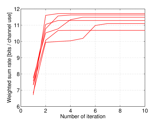
Figure 1: Convergence of Algorithm 1: $K=3$, $(N,M_{1},M_{2},M_{3})=(8,2,2,2)$, and $P_{1}=P_{2}=P_{3}=30$.

First, we verified the convergence of the overall algorithm. Fig. 1 shows the convergence behavior of Algorithm 1 for several different channel realizations when $K=3$, $(N,M_{1},M_{2},M_{3})=(8,2,2,2)$ and $P_{1}=P_{2}=P_{3}=30$. Here, we used the steepest descent method on the product manifold ${\cal M}_{i}$ with step sizes

$$0.05\times\bigg{\|}\frac{\partial}{\partial{\bf U}_{k}^{*}}\bigg{(}\sum_{i=1}^{K}w_{i}R_{i}\bigg{)}\bigg{\|}_{F}~{}~{}~{}~{}\mbox{and}~{}~{}~{}~{}0.05\times\bigg{\|}\frac{\partial}{\partial\mbox{$\bf\Lambda$}_{k}}\bigg{(}\sum_{i=1}^{K}w_{i}R_{i}\bigg{)}\bigg{\|}_{F}$$ (69)

for the $U$ and $\Lambda$ steps in our subalgorithm. The step sizes in (69) are designed to gradually reduce to zero as the subalgorithm approaches a (locally) optimal point and to show better convergence behavior near the locally optimal point. It is observed in the figure that the overall algorithm converges very fast and the number of iterations for convergence is only a few for most channel realizations in this case. Thus, the main computational time lies in the execution of the subalgorithm. Although the steepest descent based subalgorithm is used in this demonstration, different methods with faster convergence can be used [15, 21, 20].

With convergence of the algorithm confirmed, we examined the sum rate performance of the proposed beam design algorithm. Figures 2 (a) and (b) show the rate-tuples of several beam design methods for two different channel settings. We considered the single-user eigen-beamforming, the zero-forcing beamforming in addition to the proposed beam design method. For the proposed beam design method for weighted sum rate maximization, we varied the weights so that we can obtain rate-tuples at different locations. As expected, it is seen that the rate performance of the proposed method is superior to those of the eigen-beamforming and the zero-forcing. Of course, the weighted sum rate maximization can be performed in the original beam search space ${\cal Q}_{1}\times\cdots\times{\cal Q}_{K}$ by using one of gradient descent type algorithms. However, such a method is far less efficient than the proposed beam design method based on the proposed parameterization for the beam search space not losing Pareto-optimality.

(a) (b)

Figure 2: Rate pairs of several beam design methods: (a) $K=2$, $(N,M_{1},M_{2})=(6,2,2)$, $P_{1}=P_{2}=5$ and (b) $K=2$, $(M,N_{1},N_{2})=(5,2,2)$, $P_{1}=P_{2}=10$

Finally, Fig. 3 shows the sum rate performance of the algorithm w.r.t. SNR for three different system parameter settings: (1) $K=2$, $(N,M_{1},M_{2})=(5,2,2)$, (2) $K=3$, $(N,M_{1},M_{2},M_{3})=(8,2,2,1)$, and (3) $K=3$, $(N,M_{1},M_{2},M_{3})=(8,2,2,2)$. Table I summarizes the corresponding obtained rank of the converged $\mbox{$\bf\Lambda$}_{i}$, $i=1,\cdots,K$, by the proposed beam design algorithm. Note that in the low SNR regime indeed the proposed beam design algorithm does not yield a beamformer with the maximum available DoFs of $M_{i}$ for all $i$. Futhermore, it tells who should not use the available (single-user) full DoFs for sum rate maximization. It is expected that at low SNR the optimal strategy does not use maximum DoFs since all power can be allocated in the best direction, as in the single-user MIMO case. Due to the separate parameterization for ${\bf U}_{i}$ and $\mbox{$\bf\Lambda$}_{i}$ in the beam search space ${\cal M}_{i}$, our algorithm can clearly identify the optimal rank of the beamforming matrix by checking the rank of $\mbox{$\bf\Lambda$}_{i}$.

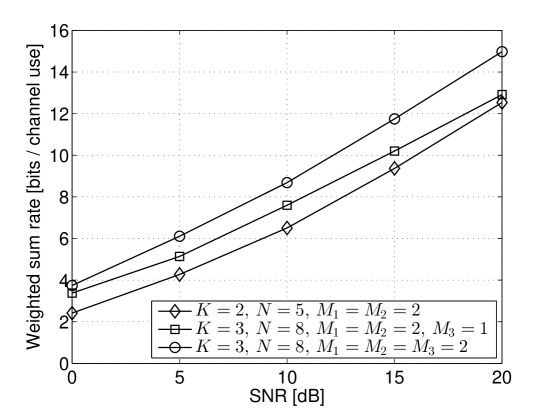
Figure 3: Performance of the proposed method: Sum rate with respect to SNR

SNR [dB]	0	5	10	15	20
$K=2$, $N=5,M_{1}=2,M_{2}=2$	$(1,2)$	$(1,2)$	$(1,2)$	$(2,2)$	$(2,2)$
$K=3$, $N=8,M_{1}=2,M_{2}=2,M_{3}=1$	$(1,2,1)$	$(1,2,1)$	$(2,2,1)$	$(2,2,1)$	$(2,2,1)$
$K=3$, $N=8,M_{1}=2,M_{2}=2,M_{3}=2$	$(2,1,1)$	$(2,2,1)$	$(2,2,2)$	$(2,2,2)$	$(2,2,2)$

TABLE I: The obtained number of data streams for Fig. 3: $d_{i}$ in $(d_{1},d_{2},d_{3})$ in the table denotes the obtained rank of $\mbox{$\bf\Lambda$}_{i}$ for transmitter-receiver pair $i$

VI Conclusion

We have considered the Pareto-optimal beam structure for multi-user multiple-input multiple-output (MIMO) interference channels and have provided a necessary condition for any Pareto-optimal transmit signal covariance matrix for the $K$-pair Gaussian $(N,M_{1},\cdots,M_{K})$ interference channel. We have shown that any Pareto-optimal transmit signal covariance matrix at a transmitter should have its column space contained in the union of the eigen-spaces of the channel matrices from the transmitter to all receivers. Based on this necessary condition, we have proposed an efficient parameterization for the beam search space, given by the product manifold of a Stiefel manifold and a subset of a hyperplane. Based on the proposed parameterization, we have developed a very efficient beam design algorithm by exploiting the geometrical structure of the beam search space and existing tools for optimization on Stiefel manifolds. We hope that the results in this paper would be helpful for efficient intercell interference control based on MIMO antenna technologies in current and future cellular networks.

References

• [1] V. R. Cadambe and S. A. Jafar, “Interference alignment and degrees of freedom of the $K$-user interference channel,” IEEE Trans. Inf. Theory, vol. 54, pp. 3425 – 3441, Aug. 2008.
• [2] E. Jorswieck, E. Larsson, and D. Danev, “Complete characterization of the Pareto boundary for the MISO interference channel,” IEEE Trans. Signal Process., vol. 56, pp. 5292 – 5296, Oct. 2008.
• [3] E. Björnson, R. Zakhour, D. Gesbert, and B. Ottersten, “Cooperate multicell precoding: Rate region characterization and distributed strategies with instantaneous and statistical CSI,” IEEE Trans. Signal Process., vol. 58, pp. 4298 – 4310, Aug. 2010.
• [4] R. Zhang and S. Cui, “Cooperative interference management with MISO beamforming,” IEEE Trans. Signal Process., vol. 58, pp. 5450 – 5458, Oct. 2010.
• [5] R. Zakhour and D. Gesbert, “Distributed multicell-MISO precoding using the layered virtual SINR framework,” IEEE Trans. Wireless Commun., vol. 9, pp. 2444 – 2448, Aug. 2010.
• [6] R. Mochaourab and E. Jorswieck, “Optimal beamforming in interference networks with perfect local channel information,” IEEE Trans. Signal Process., vol. 59, pp. 1128 – 1141, Mar. 2011.
• [7] X. Shang, B. Chen, and H. V. Poor, “Multiuser MISO interference channels with single-user detection: Optimality of beamforming and the achievable rate region,” IEEE Trans. Inf. Theory, vol. 57, pp. 4255 – 4273, Jul. 2011.
• [8] J. Park, G. Lee, Y. Sung, and M. Yukawa, “Coordinated beamforming with relaxed zero forcing: The sequential orthogonal projection combining method and rate control,” ArXiv pre-print cs.IT/1203.1758, Mar. 2012.
• [9] E. Björnson, M. Bengtsson, and B. Ottersten, “Pareto characterization of the multicell MIMO performance region with simple receivers,” IEEE Trans. Signal Process., vol. 60, pp. 4464 – 4469, Aug. 2012.
• [10] Z. Chen, S. A. Vorobyov, C.-X. Wang, and J. Thompson, “Pareto region characterization for rate control in MIMO interference systems and Nash bargaining,” to appear in IEEE Trans. Autom. Control.
• [11] P. Cao, E. Jorswieck, and S. Shi, “On the Pareto boundary for the two-user single-beam MIMO interference channel,” ArXiv pre-print cs.IT/1202.5474, Feb. 2012.
• [12] T. L. Marzetta, “Noncooperative celular wireless with unlimited number of base station antennas,” IEEE Trans. Wireless Commun., vol. 9, pp. 3590 – 3600, Nov. 2010.
• [13] F. Rusek, D. Persson, B. Lau, E. Larsson, T. Marzetta, O. Edfor, and F. Tufvesson, “Scaling up MIMO: Opportunities and challenges with very large arrays,” ArXiv pre-print cs.IT/1201.3210, Jan. 2012.
• [14] J. Lindblom, E. Larsson, and E. Jorswieck, “Parametrization of the MISO IFC rate region: The case of partial channel state information,” IEEE Trans. Wireless Commun., vol. 9, pp. 500 – 504, Feb. 2010.
• [15] R. A. Absil, R. Mahony, and R. Sepulchre, Optimization Algorithms on Matrix Manifolds, Princeton, NJ: Princeton University Press, 2007.
• [16] E. Jorswieck and E. Larsson, “The MISO interference channel from a game-theoretic perspective: A combination of selfishness and altruism achieves Pareto optimality,” in Proc. of 2008 IEEE ICASSP, (Las Vegas, NV), pp. 2805 – 2808, Apr. 2008.
• [17] A. Edelman, T. A. Arias, and S. T. Smith, “The geometry of algorithms with orthogonality constraints,” SIAM J. Matrix Anal. Appl., vol. 20, no. 2, pp. 303 – 353, 1998.
• [18] W. M. Boothby, An Introduction to Differential Manifolds and Riemannian Geometry, 2nd Ed., Academic Press, 2002.
• [19] M. P. Do Carmo, Riemannian Geometry, Boston, MA:Birkhauser, 1992.
• [20] J. H. Manton, “Optimization algorithms exploiting unitary constraints,” IEEE Trans. Signal Process., vol. 50, pp. 635 – 650, Mar. 2002.
• [21] Z. Wen and W. Yin, “A feasible method for optimization with orthogonality constraints,” Technical Report, Rice University, 2010
• [22] S. Kay, Fundamentals of Statistical Signal Processing: Estimation Theory, Englewood Cliffs, NJ:Prentice Hall, 1993.