Parity breaking and scaling behavior in light-matter interaction

Abstract

The light-matter interaction described by Rabi model and Jaynes-Cummings (JC) model is investigated by parity breaking as well as the scaling behavior of ground-state population-inversion expectation. We show that the parity breaking leads to different scaling behaviors in the two models, where the Rabi model demonstrates scaling invariance, but the JC model behaves in cusp-like way. Our study helps further understanding rotating-wave approximation and could present more subtle physics than any other characteristic parameter for the difference between the two models. More importantly, our results could be straightforwardly applied to the understanding of quantum phase transitions in spin-boson model. Furthermore, the scaling behavior is observable using currently available techniques in light-matter interaction.

The Rabi model rabi presents an important prototype for the interaction between a single two-level system (e.g., a spin) and a quantum bosonic field, which has been widely applied to almost every subfield of physics, e.g., the cavity quantum electrodynamics (QED) and the exciton-photon interaction. Under the rotating-wave approximation (RWA), the Rabi model is reduced to the Jaynes-Cummings (JC) model jc in which counter-rotating effects are neglected by the assumption of large detuning and small Rabi frequency. It is generally believed that the RWA works worse and worse with the increase of the Rabi frequency sk . So, in the case of strong spin-field coupling, the Rabi model, rather than the JC model, is required. The differences between the two models have been studied by solving the eigenenergies non-rwa ; liu1 , the dynamics non-rwa-1 ; dyna , the Berry phase berry and so on.

Going beyond the interaction between a single spin-1/2 and a single quantum mode, the Rabi model has been extended to a big-spin (S$>$1/2) system muiti or many spin-1/2 experiencing a single quantum mode, the latter of which is called Dicke model dicke . It has been shown that the RWA introduced in the Hamiltonian of the Dicke model brings about completely different phenomena from the non-RWA case in the quantum phase transition buzek ; zhang . Besides, we may also consider a single spin-1/2 interacting with a multi-mode quantum bosonic field, called spin-boson model leggett ; weiss , to describe the dissipation of a single spin under the bosonic bath. The spin-boson models with and without the RWA demonstrate different behaviors in the spin dissipation hur .

We focus in the present work on the scaling behaviors in the Rabi and JC models, which could present us more subtle physics and more evident difference than the solutions of eigenenergies, geometric phases and dynamical properties. The different scaling behaviors are relevant to different symmetries and can be understood by parity breaking. Specifically, we show that the scaling invariance exists only in the Rabi model. In contrast, the scaling behavior in JC model behaves much differently with the change of some characteristic parameters, such as the detuning. So the difference between the two models turns to be more evident in the observation of the scaling behavior because of the significant change of the symmetries in the two models due to the introduction of the local bias field. By extending the idea to the multi-mode case, we may discover the deeper physics hidden in the quantum phase transitions in spin-boson model. More importantly, these scaling behaviors are strongly relevant to the dynamics of the spin, which could be observed in some experimentally available systems, such as the circuit QED, the trapped ion and the nanomechanical systems.

We get started from the following Hamiltonian ($\hbar=1$ throughout the work) explain ,

$$H_{sb}=-\frac{\Delta}{2}\sigma_{x}+\frac{\varepsilon}{2}\sigma_{z}+\omega a^{\dagger}a+\lambda(a+a^{\dagger})\sigma_{z},$$ (1)

where $\Delta$ and $\varepsilon$ are the tunneling and the local bias field, respectively, $\omega$ and $a^{\dagger}$ ($a$) are frequency and the creation (annihilation) operator of the single-mode bosonic field, and $\lambda$ is the Rabi frequency. $\sigma_{z,x}$ are the usual Pauli operators for the spin-1/2 and $\sigma_{x}=\sigma_{+}+\sigma_{-}$ with $\sigma_{\pm}=(\sigma_{x}\pm i\sigma_{y})/2$. Compared to the standard form of the Rabi model, Eq. (1) owns an additional term, i.e., the local bias, which brings in new and more interesting physics. As discussed later, Eq. (1) connects directly to the spin-boson model and to other currently experimentally achieved systems.

Eq. (1) can be diagonalized by displaced coherent states. The eigenfunction of $H_{sb}$ has the form berry ; liu1

$$|\tilde{\Psi}\rangle=\sum_{n}\left(\begin{array}[]{l}~{}~{}~{}~{}~{}~{}~{}~{}~{}~{}~{}c_{n}|n\rangle_{A}\\ (-1)^{n+1}d_{n}|n\rangle_{B}\end{array}\right),$$

where $c_{n}$ and $d_{n}$ are coefficients to be determined later, $|n\rangle_{A}=\frac{e^{-q^{2}/2}}{\sqrt{n!}}(a^{\dagger}+q)^{n}e^{-qa^{\dagger}}|0\rangle$ and $|n\rangle_{B}=\frac{e^{-q^{2}/2}}{\sqrt{n!}}(a^{\dagger}-q)^{n}e^{qa^{\dagger}}|0\rangle$ are the displaced coherent states with the displacement variable $q=\lambda/\omega$. The complete eigensolution of H_sb can be obtained from the Schr$\stackrel{{\scriptstyle..}}{{o}}$dinger equation (See Appendix A) explain1 . We check the ground-state population-inversion $\langle\sigma_{z}\rangle$, which is,

$$\langle\sigma_{z}\rangle=(c_{0}^{-})^{2}-(d_{0}^{-})^{2}=\frac{-\kappa}{\sqrt{\kappa^{2}+e^{-4\beta}}},$$ (2)

where $\beta=q^{2}$, $\kappa=\varepsilon/\Delta$, and $c_{0}^{-}$ and $d_{0}^{-}$ are defined in Appendix A. In contrast to the perturbation solutions published previously pertur , we obtain Eq. (2) by considering the zeroth-order elements in the diagolization of the matrix of Eq. (1) liu1 . In the present case of very small $\Delta$, this consideration is a very good approximation of the complete solution to Eq. (1) explain2 .

We first perform the second derivative of $\langle\sigma_{z}\rangle$ with respect to $\beta$, which yields a reflection point $\beta_{c}=-\ln(2\kappa^{2})/4$ and thereby Eq. (2) is rewritten as

$$\langle\sigma_{z}\rangle=\frac{-\kappa}{\sqrt{\kappa^{2}+e^{\beta^{{}^{\prime}}\ln(2\kappa^{2})}}},$$ (3)

under the scaling transformation $\beta^{\prime}=\beta/\beta_{c}$. From the definition of $\beta_{c}$, we require $\kappa\neq 0$, i.e., $\epsilon\neq 0$ in the present calculation. For a fixed value of $\kappa$, the population-inversion $\langle\sigma_{z}\rangle$ in Eq. (3) is only relevant to $\beta^{{}^{\prime}}$, rather than to other characteristic parameters (See Fig. 1(a)). So $\beta_{c}$ can be regarded as a scale of the Rabi model. In addition, if we set $\beta^{{}^{\prime}}=1$, the population-inversion $\langle\sigma_{z}\rangle$ turns to be a constant $-1/\sqrt{3}$, implying a fixed crossing point with variation of $\beta^{{}^{\prime}}$. It is more interesting to demonstrate the scaling behavior of the population-inversion $\langle\sigma_{z}\rangle$ with a displaced scaling $\beta^{{}^{{}^{\prime\prime}}}=(\beta-\beta_{c})/\sqrt{27}$. Since $\langle\sigma_{z}(\beta^{{}^{{}^{\prime\prime}}})\rangle=-1/\sqrt{1+2e^{-12\sqrt{3}\beta^{{}^{{}^{\prime\prime}}}}}$, which is independent of $\kappa$ under the scaling transformation, the population-inversion $\langle\sigma_{z}\rangle$ with respect to $\beta^{{}^{{}^{\prime\prime}}}$, remains unchanged for different parameters $\kappa$, as shown in Fig. 1(b).

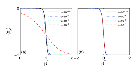
Figure 1: (color online) Scaling behavior of the ground-state population-inversion. (a) As a function of $\beta^{\prime}$ which has a fixed point; (b) As a function of $\beta^{\prime\prime}$ which remains unchanged.

It has been generally considered that the scaling invariance is relevant to the critical points of quantum phase transition in spin-boson model hur . Despite only for the interaction between a single spin and a single mode of the quantized field, the scaling behavior we show here can discover the physical insight in the fundamental element of the spin-boson model, which is resulted from the parity breaking regarding the parity operator $\Pi=\sigma_{x}e^{i\pi a^{\dagger}a}$. If we denote the case of $\epsilon=0$ in Eq. (1) by $H_{sb}^{{}^{\prime}}$, we have $[H_{sb}^{{}^{\prime}},\Pi]=0$, with the ground state of their common eigenfunction to be $|\psi_{0}^{-}\rangle=-\frac{1}{\sqrt{2}}\left(\begin{array}[]{l}|0\rangle_{A}\\ |0\rangle_{B}\end{array}\right)$satisfying $\Pi|\psi_{0}^{-}\rangle=|\psi_{0}^{-}\rangle$, i.e., an even parity state of $\Pi$. The even parity breaks down in the variation from $\varepsilon=0$ to $\epsilon\neq 0$ because the Hamiltonian $H_{sb}$ never commutes with the parity operator $\Pi$, i.e., $[H_{sb},\Pi]\neq 0$. This parity-breaking case plotted in Fig. 1(a) (except the point $\beta^{\prime}=0$) demonstrates the abrupt variation of $\langle\sigma_{z}\rangle$ from 0 to -1 at $\kappa$ approaching 0, corresponding to the translation from spin non-localization (i.e., superposition of the spin-up and spin-down) to spin localization (i.e., the spin down). This peculiar scaling behavior is very analogous to the critical point behavior in quantum phase transition of the spin-boson model (See Fig. 3 in hur ). More interestingly, this sharp scaling variation induced by the parity breaking could appear for larger $\kappa$ (e.g., $\kappa=$0.1) under a scaling displacement (Fig. 1(b)).

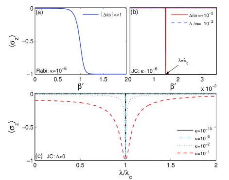
Figure 2: (color online) (a) The ground-state population-inversion for $H_{sb}$ as a function of $\beta^{\prime}$ with $\kappa=10^{-6}$. (b) The ground-state population-inversion for $H_{jc}$ as a function of $\beta^{\prime}$ for $\Delta>0$ (the red solid line with cusp-like scaling behavior) and for negative $\Delta$ (the blue dashed line with no scaling behavior) with $\kappa=10^{-6}$. (c) The cusp-like scaling behavior of the ground-state population-inversion for $H_{jc}$ as a function of $\lambda/\lambda_{c}$ with $\Delta>0$ for $\kappa=10^{-10}$ (the black solid line), $\kappa=10^{-6}$ (the blue dashed-dotted line), $\kappa=10^{-2}$ (the pink dotted line), and $\kappa=10^{-1}$ (the red dashed line). For convenience of comparison between (b) and (c), we label $\lambda_{c}$ in (b).

To better understand the parity breaking in the Rabi model, we may consider the same treatment for the JC model. In the case of $\epsilon=0$, the ground-state of the JC model is usually of certain parity, and experiences energy level crossing. In the case of $\epsilon\neq 0$, however, the parity breaks down and level crossing turns to level avoided-crossing (See Appendix B). But different from the scaling invariance in the Rabi model, the variation of $\langle\sigma_{z}\rangle$ with respect to $\beta^{\prime}$ behaves with a cusp in the JC model (See Fig. 2(a) and 2(b) for comparison between the two models). It implies that the spin is always in non-localization except the rare cases near the critical point $\lambda_{c}$ for localization. For $\kappa=10^{-6}$, we have $\beta_{c}=6.73$, corresponding to $\lambda=2.59\omega$ in the Rabi model and to $\lambda=0.09\omega$ in the JC model. These are reasonable values for the parameters in the two models. For a more clarified demonstration, we plot in Fig. 2(c) $\langle\sigma_{z}\rangle$ versus $\lambda/\lambda_{c}$, where $\lambda_{c}=\sqrt{\omega\Delta}$ takes values much smaller than $\beta_{c}$. So we could have a zooming-in picture for the variation of $\langle\sigma_{z}\rangle$, which shows strong relevance to $\kappa$. The cusp-like behavior is evidently induced by the parity breaking (i.e., for $\kappa$ very close to zero).

The results above remind us of the role the counter-rotating terms playing in the light-matter interaction. For the parity operator $\Pi$ with respect to H_sb, we have $\Pi^{\prime}=U^{\dagger}\Pi U=-\sigma_{z}e^{i\pi a^{\dagger}a}$ for H_jc where $U$ is defined in explain . If we neglect the terms regarding $\epsilon$, we have $[\Pi,H^{\prime}_{sb}]=0$ and $[\Pi^{\prime},H_{rjc}]=0$. But this does not mean that the counter-rotating terms have no extra influence on the symmetry in the Rabi model compared to the JC model. First, in the case of $\epsilon=0$, the ground-state of the JC model (for $\Delta>$0) experiences a translation from the even parity to the odd in the increase of the coupling $\lambda$, but the ground-state of the Rabi model only stays in the even parity. This could be understood physically from whether the energy level crossing happens or not. But the deeper physics is the different parity behaviors in both models, which yield different dynamics dyna . Second, for $\epsilon\neq 0$, only energy avoided-crossing occurs in either of the models (See Appendix B). We may discern the two models by scaling behaviors around the critical point of the parity breaking, which presents the difference between the two models more evidently than other quantities non-rwa ; liu1 ; berry . This idea can be straightforwardly extended to the spin-boson model: The difference between the quantum phase transitions with and without RWA should be relevant to different critical behaviors around the parity breaking points.

Eq. (1) can be generated in various systems. Since $\langle\sigma_{z}\rangle$ is observable experimentally, we may demonstrate the scaling behaviors using currently available techniques. We first check the circuit QED system with a superconducting qubit strongly coupled to a microwave resonator mode via external driving, which can be described by cir1 ; cir2 ; ball $H_{qed}=\frac{\omega_{q}}{2}\sigma_{z}+\omega_{b}b^{\dagger}b+G(b\sigma_{+}+b^{\dagger}\sigma_{-})+\Omega_{1}(e^{i\omega_{1}t}\sigma_{-}+e^{-i\omega_{1}t}\sigma_{+})-\Omega_{2}(e^{i\omega_{2}t}\sigma_{-}+e^{-i\omega_{2}t}\sigma_{+})$, where $\omega_{q}$ and $\omega_{b}$ are, respectively, the qubit and microwave photon frequencies with $G$ the qubit-photon coupling strength. $b$ ($b^{\dagger}$) stands for the annihilation (creation) operator of the microwave photon. $\sigma_{z,\pm}$ are usual Pauli operators for the superconducting qubit. $\Omega_{j}$ and $\omega_{j}$ are the amplitude and frequency of the $j$th driving field ($j=$1, 2). We assume $\Omega_{1}\gg\Omega_{2}$, $G$ and in the rotating frame first with the driving field $\omega_{1}$ and then with a large frequency $\Omega_{3}$ comparable to $\Omega_{1}$, we may obtain an effective Hamiltonian by setting $\Omega_{3}=(\omega_{1}-\omega_{2})/2$ and neglecting fast oscillating terms, $H_{eff}=\frac{\Omega_{2}}{2}\sigma_{z}+\frac{(\Omega_{1}-\Omega_{3})}{2}\sigma_{x}+(\omega_{b}-\omega_{1})b^{\dagger}b+\frac{G}{2}(b+b^{\dagger})\sigma_{x}$, which can be used to simulate the Rabi model and JC model by tuning the characteristic parameters. For the Rabi model, to meet the condition $\Omega_{2}\ll(\omega_{b}-\omega_{1})\sim G/2$, we can adopt following experimental parameters as $\omega_{q}=2\pi\times 6.02$ GHz, $\omega_{b}=2\pi\times 6.02$ GHz, $\omega_{1}=2\pi\times 6$ GHz, $\omega_{2}=2\pi\times 4$ GHz, and a tunable $G>2\pi\times 40$ MHz. Besides, we may assume the driving fields with the amplitudes $\Omega_{3}=2\pi\times 1$ GHz and $\Omega_{2}=2\pi\times 0.4$ MHz. $(\Omega_{1}-\Omega_{3})$ can change from zero to $2\pi\times$20 kHz, which are realistic values using state-of-the-art circuit-QED technology super1 ; super2 . While for JC model, the result can be obtained by reducing the coupling strength to $G<2\pi\times 4$ MHz and remaining other parameters unchanged.

Similarly, Eq. (1) can also be implemented by a diamond nitrogen-vacancy center (i.e., a single spin) coupled by a nanomechanical resonator rabl , in which the strong coupling due to magnetic field gradient from the tip of the resonator can be of the order of hundreds of kHz tip . Under a driving on the spin, we may have in the rotating frame with respect to the driving frequency $H_{nv}=(\Omega^{\prime}/2)\sigma_{x}+(\Delta^{\prime}/2)\sigma_{z}+\omega_{m}a^{\dagger}a+\lambda^{\prime}(a^{\dagger}+a)\sigma_{z}$ with $\Delta^{\prime}$ the detuning of the two-level resonance frequency to the the driving frequency, $a^{\dagger}(a)$ for the vibration of the resonator with frequency $\omega_{m}$, and $\lambda^{\prime}$ and $\Omega^{\prime}$ being, respectively, the magnetic coupling and the driving strength. By tuning the driving strength and the driving frequency, we may simulate the Rabi model (with $\Omega^{\prime}\ll\omega_{m}\sim\lambda^{\prime}$) and the JC model (with $\omega_{m}\gg\lambda^{\prime}$) from $H_{nv}$ as our will.

Simply speaking, once the strong coupling between the spin and the quantum field is achieved, the two models can be generated from Eq. (1) by balancing the vibrational frequency and the spin-field coupling. In this sense, we may also consider a single trapped ultracold ion experiencing irradiation of traveling lasers. Under some unitary transformations liu0 , we have $H_{ion}=-(\tilde{\Omega}/2)\sigma_{x}+\tilde{\epsilon}\sigma_{z}+\tilde{\nu}a^{\dagger}a+\tilde{g}(a^{\dagger}+a)\sigma_{z}$ explain3 , where $\sigma_{x,z}$ are the usual Pauli operators for two internal levels of the ion, $a^{\dagger}(a)$ is for the vibration of the ion, $\tilde{\Omega}$ and $\tilde{\nu}$ are the Rabi frequency and the trap frequency, $\tilde{\epsilon}$ is relevant to detuning and $\tilde{g}=\tilde{\nu}\eta/2$ with the Lamb-Dicke parameter $\eta$. Since $H_{ion}$ works for any value of $\eta$, we may have $\tilde{\Omega}\ll\tilde{\nu}\approx\tilde{g}$ by using weak laser irradiation and deep trap potential, which is for the Rabi model, and have $\tilde{\nu}\gg\tilde{g}$ by restricting the ion within Lamb-Dicke regime, corresponding to the JC model. The typical trap frequency $\tilde{\nu}$ varies from hundreds of kHz to several MHz and Rabi frequency $\tilde{\Omega}$ is adjustable by laser irradiation (up to hundreds of kHz) blattm .

In conclusion, we have investigated the scaling behaviors of ground-state population-inversion in light-matter interaction, which is relevant to the parity breaking. The different scaling behaviors can be used to not only identify the difference between the Rabi model and the JC model, but also demonstrate the change of the symmetry in the system. We have also discussed the experimental feasibility of our study in different systems using currently available technology. The present idea could be straightforwardly extended to the study of spin-boson model for possible quantum phase transitions induced by the parity breaking.

This work is supported by NFRPC (Grant No. 2012CB922102) and by NNSFC (Grants No. 11274352, No. 11147153, No. 11004226, and No. 11147153).

APPENDIX

A. Our eigensolution to the Rabi model

Taking $|\tilde{\Psi}\rangle$ into the Schr$\stackrel{{\scriptstyle..}}{{o}}$dinger equation of H_sb, we obtain a set of equations $[\omega(m-q^{2})+\frac{\epsilon}{2}]c_{m}+\frac{\Delta}{2}\sum_{n}d_{n}D_{m,n}=Ec_{m}$ and $[\omega(m-q^{2})-\frac{\epsilon}{2}]d_{m}+\frac{\Delta}{2}\sum_{n}c_{n}D_{m,n}=Ed_{m}$, with $D_{m,n}=e^{-2q^{2}}\sum_{k=0}^{\min[m,n]}(-1)^{-k}\frac{\sqrt{m!n!}(2q)^{m+n-2k}}{(m-k)!(n-k)!k!}$ berry ; liu0 ; liu1 . In our case with the condition $\Delta/\omega\ll 1$, the terms of $D_{m,n}$ with $m\neq n$ play negligible roles in the equations compared to other terms with $m=n$. So the equations above can be simplified to the case remaining the terms of $m=n$, which yields following analytical solutions, that is, the eigenenergies $E_{m}^{\pm}=\omega(m-q^{2})\pm\sqrt{\epsilon^{2}+\Delta^{2}D_{m,m}^{2}}/2$, and the coefficients $c_{m}^{\pm}=\mu_{m}^{\pm}/\sqrt{1+(\mu_{m}^{\pm})^{2}}$ and $d_{m}^{\pm}=1/\sqrt{1+(\mu_{m}^{\pm})^{2}}$ with $\mu_{m}^{\pm}=[\epsilon\pm\sqrt{\epsilon^{2}+\Delta^{2}D_{m,m}^{2}}]/(\Delta D_{m,m})$. The eigenfunction of the ground-state is $|\psi_{0}^{-}\rangle=-\left(\begin{array}[]{l}|0\rangle_{A}\\ |0\rangle_{B}\end{array}\right)/\sqrt{2}$ since $E_{0}^{-}$ is smaller than $E_{0}^{+}$.

B. Avoided-crossing around the critical points of parity breaking

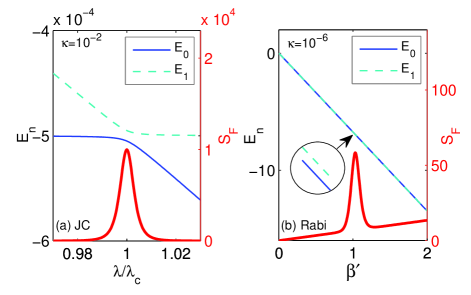
Figure 3: (color online) Eiegenenergies and fidelity susceptibility S_F. (a) for JC model with the additional term $\epsilon/2$, no level crossing appears and sudden change in fidelity susceptibility occurs around $\lambda=\lambda_{c}$; (b) for Rabi model with the additional term $\epsilon/2$, no level crossing appear and sudden change in fidelity susceptibility occurs around $\beta^{\prime}=1$.

In JC model, there are level crossings in the ground state with the excited states in different parities. So a level crossing means the change of the parity in the ground state. In contrast, there are only avoided-crossings of levels in Rabi model, which yield unchanged parity. So the RWA effect can be reflected from the parity change. In our present work, however, due to the introduction of the additional term regarding $\epsilon/2$, no level crossing exists anymore in the JC model, but only avoided-crossings, as shown in Fig. 3. So we may consider other characteristic properties, such as scaling behavior, for understanding the effect of the RWA. Our results show that the scaling behavior can present more evident difference than any other characteristic parameters used previously. More interestingly, we see in Fig. 3 the sudden change occurring in the fidelity susceptibility (S_F) fs around the critical point of the parity breaking, which also happens in the spin-boson model around the critical point of quantum phase transition sf1 . This implies that the deeper physics for quantum phase transition in the multi-mode case might be also due to the parity breaking. The fidelity susceptibility is defined by $S_{F}(\lambda_{1})=\sum_{n\neq 0}\frac{|\langle\phi_{n}(\lambda_{1})|H_{1}|\phi_{0}(\lambda_{1})\rangle|^{2}}{[E_{n}(\lambda_{1})-E_{0}({\lambda_{1}})]^{2}}$, where $H=H_{0}+\lambda_{1}H_{1}$ with $\lambda_{1}$ the order parameter, $H$ is the hamiltonian under our consideration. $\phi_{k}$ and $E_{k}$ are k$th$ eigenstate and the corresponding eigenenergy. In our treatment, we take spin-field interaction as $H_{1}$.

References

- (1) I. I. Rabi, Phys. Rev. 49, 324 (1936); ibid 51, 652 (1937).
- (2) E. T. Jaynes and F. W. Cummings, Proc. IEEE 51, 89 (1963).
- (3) B. W. Shore and P. L. Knight, J. Mod Opt. 40, 1195 (1993).
- (4) M. D. Crisp, Phys. Rev. A 43, 2430 (1991); E. K. Irish, Phys. Rev. Lett. 99, 173601 (2007); D. Braak, Phys. Rev. Lett. 107, 100401 (2011).
- (5) T. Liu, K. L. Wang and M. Feng, Europhys. Lett. 86, 54003 (2009).
- (6) S. J. D. Phoenix, J. Mod. Optics 3, 127 (1989); H. Zheng, S. Y. Zhu and M. S. Zubairy, Phys. Rev. Lett. 101, 200404 (2008); J. Casanova, G. Romero, I. Lizuain, J. J. Garcia-Ripoll and E. Solano, Phys. Rev. Lett. 105, 263603 (2010).
- (7) I.D. Feranchuk and A.V. Leonov, Phys. Lett. A 373, 4113 (2009); ibid 375, 385 (2011); F. A. Wolf, M. Kollar, and D. Braak, Phys. Rev. A 85, 053817 (2012); F. A. Wolf, F. Vallone, G. Romero, M. Kollar, E. Solano, D. Braak, eprint, quant-ph/1211.6469.
- (8) T. Liu, M. Feng, and K. L. Wang, Phys. Rev. A 84, 062109 (2011).
- (9) V. V. Albert, Phys. Rev. Lett. 108, 180401 (2012).
- (10) R. H. Dicke, Phys. Rev. 93, 99 (1954).
- (11) V. Buzek, M. Orszag, and M. Rosko, Phys. Rev. Lett. 94, 163601 (2005); K. Rzazewski and K. Wodkiewicz, Phys. Rev. Lett. 96, 089301 (2006).
- (12) Y. Y. Zhang, T. Liu, Q. H. Chen and K. L. Wang, Opt. Commun. 283, 3459 (2010).
- (13) A. J. Leggett, S. Chakravarty, A.T. Dorsey, M. P. A. Fisher, A. Garg, W. Zwerger, Rev. Mod. Phys. 59, 1 (1987).
- (14) U. Weiss, Quantum dissipative Systems (World Scientific, Singapore, 1999).
- (15) K. Le Hur, Ann. Phys. 323, 2208 (2008).
- (16) The Hamiltonian is a simplified form of the spin-boson model with the single mode of the bosonic field, which is physically equivalent to the Rabi model with an additional local bias. Using a unitary transformation , we may transform to , which is the standard Hamiltonian of the Rabi model, in addition to a tunneling term. The Rabi model includes both the rotating terms (, ) and the counter-rotating terms (, ). If the counter-rotating terms are dropped, the model is reduced to a general JC model with a tunneling term. In our calculation, we present the results regarding Rabi model from Hsb in Eq. (1), and obtain the results regarding JC model from following the unitary rotation .
- (17) We consider the solution of the Schrödinger equation in the case of , which is based on following reasons. First, it simplifies the solution and leads to analytical expressions of eigenenergy and eigenfunction. This condition is also experimentally acceptable. Second, The small value of can somewhat reflect the physics related to the parity operator , which commutes with Hsb in the case of . So besides the parity breaking regarding under our consideration, the model also experiences another parity breaking if we change from zero to non-zero. But we only focus on the parity breaking regarding in the present work because we are considering the bias field acting on a Rabi or JC model. The physics related to the parity operator will be discussed in details in a separate paper.
- (18) I. D. Feranchuk, L. I. Komarov and A. P. Ulyanenkov J. Phys. A 29, 4035 (1996).
- (19) We have also made numerical calculation in saturation for Fig. 1, which presents the same results as from Eq. (2).
- (20) A. Blais, R.-S. Huang, A. Wallraff, S. M. Girvin, and R. J.Schoelkopf, Phys. Rev. A 69, 062320 (2004).
- (21) A. Wallraff, D. I. Schuster, A. Blais, L. Frunzio, R.-S. Huang, J. Majer, S. Kumar, S.M. Girvin, and R. J. Schoelkopf, Nature (London) 431, 162 (2004).
- (22) D. Ballester, G. Romero, J. J. Garcia-Ripoll, F. Deppe and E. Solano, Phys. Rev. X 2, 021007 (2012).
- (23) P. Forn-Daz, J. Lisenfeld, D. Marcos, J. J. Garca-Ripoll, E. Solano, C. J. P. M. Harmans, and J. E. Mooij, Phys. Rev. Lett. 105, 237001 (2010).
- (24) T. Niemczyk, F. Deppe, H. Huebl, E. P. Menzel, F. Hocke, M. J. Schwarz, J. J. Garcia-Ripoll, D. Zueco, T. Hmmer, E. Solano, A. Marx, and R. Gross, Nat. Phys. 6, 772 (2010).
- (25) P. Rabl, P. Cappellaro, M. V. Gurudev Dutt, L. Jiang, J. R. Maze and M. D. Lukin, Phys. Rev. B 79, 041302(R) (2009).
- (26) H. J. Mamin, M. Poggio, C. L. Degen and D. Rugar, Nat. Nanotechnol. 2, 301 (2007).
- (27) T. Liu, K. L. Wang, and M. Feng, J. Phys. B 40, 1967 (2007);
- (28) In comparison to Eq. (3) in liu0 , we omit the constant term and make up the trap frequency .
- (29) D. Leibfried, R. Blatt, C. Monroe and D. Wineland, Rev. Mod. Phys. 75, 281 (2003).
- (30) W. L. You, Y. W. Li, and S. J. Gu, Phys. Rev. E 76, 022101 (2007).
- (31) T. Liu, Y. Y. Zhang, Q. H. Chen, and K. L. Wang, Phys. Rev. A 80, 023810 (2009).