Correlation lengths of the repulsive one-dimensional Bose gas

Abstract

We investigate the large-distance asymptotic behavior of the static density-density and field-field correlation functions in the one-dimensional Bose gas at finite temperature. The asymptotic expansions of the Bose gas correlators are obtained performing a specific continuum limit in the similar low-temperature expansions of the longitudinal and transversal correlation functions of the XXZ spin chain. In the lattice system the correlation lengths are computed as ratios of the largest and next-largest eigenvalues of the XXZ spin chain quantum transfer matrix. In both cases, lattice and continuum, the correlation lengths are expressed in terms of solutions of Yang-Yang type YY4 non-linear integral equations which are easily implementable numerically.

I Introduction

In the last decade we have witnessed significant advances in the field of trapped ultracold gases BDZ opening new avenues for the investigation of low-dimensional physical systems which can be well approximated by integrable models. The paradigmatic example is the Bose gas with contact interaction LL , also known as the Lieb-Liniger model, whose experimental realization tMSK ; tKWW1 ; tP ; tLOH ; tPRD ; tAetal has spurred renewed interest in computing physical properties which are experimentally accessible. In particular, the correlation functions, which can be measured using interference tPAE ; tIGD ; tHetal ; tDetal , analysis of particle losses tLOH ; tHetal1 , photoassociation tKWW2 , Bragg and photoemission spectroscopy DADSC ; tPetal ; tCFFFI ; tFetal1 ; tEetal , density fluctuation statistics AJKB ; JABKB ; Armijo1 ; Armijo2 , time-of-flight correlation statistics HDMBT and scanning electron microscopy GWEVBO are extremely important.

Despite the integrability of the model the calculation of the correlation functions is an extremely challenging problem which remains unsolved to this day. Significant simplifications occur in the case of infinite repulsion when the system is equivalent to free fermions. In this case the correlators can be expressed as Fredholm or Toeplitz determinants and the asymptotic behavior can be extracted from the solution of an associated Riemann-Hilbert problem Le1 ; Le2 ; VT1 ; VT2 ; JMMS ; IIK ; IIK0 ; IIK1 ; IIKV . Similar results, albeit in a non-rigorous fashion, can be derived using the replica method Ga1 .

The introduction of the algebraic Bethe ansatz (ABA) provided the necessary tools to tackle the harder problem of calculating the correlation functions of integrable models away from the free fermion point BK1 ; IK1 ; Ka ; KBI . At zero temperature, the members of the Lyon group (Kitanine, Kozlowski, Maillet, Slavnov and Terras), making use of the results obtained in KMT1 ; KMT2 ; KMST1 ; KMST2 ; KKMST2 derived in KKMST the asymptotic behavior of the static density correlators in the repulsive Lieb-Liniger model and similar results for the longitudinal correlation of the XXZ spin chain. The large-distance and long-time asymptotic analysis of the density-density and field-field correlators was performed in KT ; KKK1 ; KKMSTaa . In all cases these exact results reproduce and generalize the predictions of the Tomonaga-Luttinger liquid(TLL)/Conformal Field Theory (CFT) approach BIK ; BM1 ; BM2 . A method of determining the “non-universal” prefactors appearing in the TLL/CFT expansion was introduced in SGCI1 ; SGCI2 and, also, very recently, in KKMSTa .

The temperature dependent correlation functions of a system characterized by a Hamiltonian $H$ are defined as

$$\langle\mathcal{O}\rangle_{T}=\frac{\sum\langle\Omega|\mathcal{O}|\Omega\rangle e^{-E/T}}{\sum e^{-E/T}}\,,$$ (1)

where $\mathcal{O}$ is a local operator, the sum is over all the eigenstates $|\Omega\rangle$ of the Hamiltonian, and $E$ their respective energies. The summation appearing in (1) makes the calculation of temperature dependent correlation functions extremely difficult. However, in the case of the interacting Bose gas we can circumvent this problem in two ways. First, it can be shown, see Chap. I of KBI and references therein, that in the thermodynamic limit (1) can be replaced by

$$\langle\mathcal{O}\rangle_{T}=\frac{\langle\Omega_{T}|\mathcal{O}|\Omega_{T}\rangle}{\langle\Omega_{T}|\Omega_{T}\rangle}$$ (2)

where $|\Omega_{T}\rangle$ is any of the eigenstates corresponding to thermal equilibrium. This allowed the authors of KMS1 ; KMS2 to employ a method similar with the zero temperature analysis performed in KKMST to obtain the asymptotic expansion of the generating functional of density correlators. The second method utilizes the quantum transfer matrix (QTM) and the connection between the XXZ spin chain and the one-dimensional Bose gas. Introduced and developed in MS ; K1 , the QTM, in particular its spectrum, is an extremely important tool in the investigation of temperature dependent properties of lattice systems. The free energy of the system is related to the largest eigenvalue of the QTM K1 ; K2 and the correlation lengths of the Green’s functions can be obtained as ratios of the largest and next-largest eigenvalues K2 ; KSS . At the same time the QTM is a fundamental ingredient in obtaining multiple integral representations for temperature dependent correlation functions GKS1 ; GKS2 ; KK . Even though there is no QTM equivalent for continuous systems we can use the fact that the one-dimensional Bose gas can be obtained in a specific continuum limit of the XXZ spin-chain SBGK ; KS1 . Performing this continuum limit in the non-linear integral equations (NLIEs) characterizing the eigenvalues of the XXZ spin-chain QTM we will obtain the spectrum of what we will call the “continuum” QTM, from which we can calculate the thermodynamics and the correlation lengths of the continuum system. It is precisely this method that we will use in this paper to obtain the asymptotic expansion of the temperature dependent density-density and field-field correlation functions in the one-dimensional Bose gas. We should mention that the same scaling limit was used in P1 to obtain the k-body local correlators, i.e., correlation functions of the type $\langle(\Psi^{\dagger}(0))^{k}(\Psi(0))^{k}\rangle_{T}$, for $k\leq 4$ using, however, a totally different method than ours. For $k\leq 3$ local correlators were first calculated in GS1 ; KGDS ; CSZ1 ; CSZ2 ; KCI . Other important results concerning the correlation functions of the 1D Bose gas can be found in Kb ; KSa ; KKS ; EKL ; IS ; S1 ; KBI ; CC1 ; CC2 ; CCS ; GS2 ; IG1 ; KPKG ; KKG1 ; SGDVK ; CB1 ; DSGDDK ; CCGOR ; KMTa ; KMTb .

The plan of the paper is as follows. In the next section we introduce the one-dimensional Bose gas and present the asymptotic expansions for the correlation functions which constitute the main results of this paper. In Sec. III we review the XXZ spin chain and introduce the continuum limit which allows for the derivation of the Bose gas results. In Sec. IV we introduce the XXZ spin chain QTM and obtain NLIEs for the largest and next-largest eigenvalues from which the correlation lengths can be extracted. The validity of the asymptotic expansions is checked in Sec. V by comparison with the TLL/CFT predictions. Finally, the asymptotic behavior of the correlators in the Bose gas is obtained by taking the continuum limit in Sec. VI. Some technical calculations are presented in several appendices.

II The one-dimensional Bose gas and main result

We consider a one-dimensional system of bosons interacting via a $\delta$-function potential with periodic boundary conditions. The relevant Hamiltonian is

$$H_{NLS}=\int_{0}^{l}\,dx\,\left[\partial_{x}\Psi^{\dagger}(x)\partial_{x}\Psi(x)+c\Psi^{\dagger}(x)\Psi^{\dagger}(x)\Psi(x)\Psi(x)-\mu\Psi^{\dagger}(x)\Psi(x)\right]\,,$$ (3)

where $c>0$ is the coupling constant, $\mu$ the chemical potential, $l$ the length of the system and we have considered $\hbar=2m=1$, with $m$ the mass of the particles. In (3) $\Psi^{\dagger}(x)$ and $\Psi(x)$ are Bose fields satisfying the canonical commutation relations

$$[\Psi(x),\Psi^{\dagger}(x^{\prime})]=\delta(x-x^{\prime})\,,\ \ \ \ [\Psi(x),\Psi(x^{\prime})]=[\Psi^{\dagger}(x),\Psi^{\dagger}(x^{\prime})]=0\,.$$

The interacting one-dimensional Bose gas, also known as the Lieb-Liniger or the quantum Non-Linear Schrödinger (NLS) model, is solvable by Bethe ansatz LL ; G ; KBI . In the case of $n$ particles the energy spectrum is given by

$$\overline{E}(\{k\})=\sum_{j=1}^{n}\overline{e}_{0}(k_{j})\,,\ \ \ \ \ \overline{e}_{0}(k)=k^{2}-\mu\,,$$ (4)

with the quasimomenta $k_{j}$ satisfying the following set of Bethe ansatz equations (BAEs)

$$e^{ik_{j}l}=\prod_{s\neq j}^{n}\frac{k_{j}-k_{s}+ic}{k_{j}-k_{s}-ic}\,,\ \ \ \ j=1,\cdots,n\,.$$ (5)

It is useful to present the logarithmic form of the BAEs (5)

$$lk_{j}+\sum_{s=1}^{n}\overline{\theta}(k_{j}-k_{s})=2\pi m_{j}\,,$$

where $m_{j}$ are integers or half-integers and the scattering phase $\overline{\theta}(k)$ is defined by

$$\overline{\theta}(k)=i\log\left(\frac{ic+k}{ic-k}\right)\,,\ \ \ \ \lim_{k\rightarrow\pm\infty}\overline{\theta}(k)=\pm\pi\,.$$

At zero temperature and fixed number of particles $n$ the ground state is obtained when the (half) integers take the values $m_{j}=j-(n+1)/2\,,j=1,\cdots,n$ LL . In the thermodynamic limit $l,n\rightarrow\infty\,,$ with their ratio finite $\overline{D}=n/l,$ the values of the momenta $k_{j}$ condense in the interval $[-\overline{q},\overline{q}]$ called the Fermi zone or Dirac sea and the following integral equation for the density of particles in momentum space can be derived:

$$\overline{\rho}(k)-\frac{1}{2\pi}\int_{-\overline{q}}^{\overline{q}}\overline{K}(k-k^{\prime})\overline{\rho}(k^{\prime})\,dk^{\prime}=\frac{1}{2\pi}\,,\ \ \ \ \ \ \ \ \overline{K}(k-k^{\prime})=\frac{d}{dk}\overline{\theta}(k-k^{\prime})=\frac{2c}{(k-k^{\prime})^{2}+c^{2}}\,.$$ (6)

The Fermi momentum $\overline{q}$ can be obtained as a unique function of $\overline{D}$, the density of particles, via $\overline{D}=n/l=\int_{-\overline{q}}^{\overline{q}}\overline{\rho}(k)\,dk\,.$

At finite temperature the thermodynamics of the model was calculated in YY4 (for a rigorous derivation, see DLP ; KW ). The grand-canonical potential per length is given by

$$\phi(\mu,T)=-\frac{T}{2\pi}\int_{-\infty}^{+\infty}\log\left(1+e^{-\overline{\varepsilon}(k)/T}\right)\,dk\,,$$ (7)

with $\overline{\varepsilon}(k)$, the dressed energy, satisfying the Yang-Yang equation

$$\overline{\varepsilon}(k)=k^{2}-\mu-\frac{T}{2\pi}\int_{\mathbb{R}}\overline{K}(k-k^{\prime})\log\left(1+e^{-\overline{\varepsilon}(k^{\prime})/T}\right)dk^{\prime}\,.$$ (8)

II.1 Main result

The main result of this paper is the computation of the large-distance asymptotic behavior of the correlation functions in the 1D Bose gas at finite temperature. Due to the fact that the derivation of the asymptotic expansions is quite involved we prefer to present these results in the beginning of the paper. The interested reader can find the details in the following sections.

We will start with the static density-density correlation function, $\langle j(x)j(0)\rangle_{T}$, with $j(x)=\Psi^{\dagger}(x)\Psi(x)$. Consider the following set of functions $\overline{u}_{i}(k)$ satisfying the nonlinear integral equations

$$\overline{u}_{i}(k)=k^{2}-\mu+iT\sum_{j=1}^{r}\overline{\theta}(k-k^{+}_{j})-iT\sum_{j=1}^{r}\overline{\theta}(k-k^{-}_{j})-\frac{T}{2\pi}\int_{\mathbb{R}}\overline{K}(k-k^{\prime})\log\left(1+e^{-\overline{u}_{i}(k^{\prime})/T}\right)dk^{\prime}\,.$$ (9)

The $2r$ parameters, $\{k^{+}_{j}\}_{j=1}^{r}\,(\{k^{-}_{j}\}_{j=1}^{r})$ appearing in Eq. (9) are located in the upper (lower) half of the complex plane and satisfy the constraint

$$1+e^{-\overline{u}_{i}(k^{\pm}_{j})/T}=0.$$

For a given $r$, the previous equation has more than $2r$ solutions, the subscript $i$ labels all the possible choices of solutions for all $r=1,2,\cdots$. Note that the NLIEs (9) are almost identical with the Yang-Yang equation for the dressed energy (8) with the exception of the additional driving terms. The large distance asymptotic expansion for the density-density correlation function has the form

$$\langle j(x)j(0)\rangle_{T}=const+\sum_{i}\tilde{A}_{i}\,e^{-\frac{x}{\xi^{(d)}[\overline{u}_{i}]}}\,,\ \ \ \ \ x\rightarrow\infty\,,$$ (10)

where $\tilde{A}_{i}$ are distance independent amplitudes which cannot be obtained using our method and the correlation lengths are given by

$$\frac{1}{\xi^{(d)}[\overline{u}_{i}]}=-\frac{1}{2\pi}\int_{\mathbb{R}}\log\left(\frac{1+e^{-\overline{u}_{i}(k)/T}}{1+\,e^{-\overline{\varepsilon}(k)/T}}\right)\,dk-i\sum_{j=1}^{r}k^{+}_{j}+i\sum_{j=1}^{r}k^{-}_{j}\,,$$ (11)

with $\overline{\varepsilon}(k)$ the dressed energy satisfying (8). Comparison with the TLL/CFT expansion (94) and other exact results (Chap. XVII of KBI ) allows the identification of the constant term with $\langle j(0)\rangle_{T}^{2}$. The leading terms in the expansion (10) are obtained considering $r=1$ in Eq. (9) with the parameters $k^{\pm}_{1}$, satisfying $1+e^{\overline{u}_{i}(k^{\pm}_{1})/T}=0$, closest to the real axis.

A few remarks are in order. Using a different method almost identical equations were obtained by Kozlowski, Maillet and Slavnov KMS1 ; KMS2 for the generating functional of density correlators, $\langle e^{\varphi\int_{0}^{x}j(x^{\prime})\,dx^{\prime}}\rangle_{T}$, from which the density correlator can be obtained via $\langle j(x)j(0)\rangle_{T}=\frac{1}{2}\frac{\partial^{2}}{\partial x^{2}}\frac{\partial^{2}}{\partial\varphi^{2}}\left.\langle e^{\varphi\int_{0}^{x}j(x^{\prime})\,dx^{\prime}}\rangle_{T}\right|_{\varphi=0}$ . The only difference between our equations and the ones derived in KMS1 ; KMS2 is the presence of a renormalized chemical potential $\mu\rightarrow\mu+\varphi T$ in the r.h.s. of Eq. (9). As we will show in Appendix D a slight modification of our method allows for the derivation of the asymptotic expansion for the generating functional. However, in order to not confuse the reader, we prefer here and in the following sections to focus on the density and field correlators (see below) because it allows for an almost similar treatment.

In the case of the field-field correlation function $\langle\Psi^{\dagger}(x)\Psi(0)\rangle_{T}$ we introduce the set of functions $\overline{v}_{i}(k)$ satisfying the NLIEs

$$\overline{v}_{i}(k)=k^{2}-\mu\pm i\pi T+iT\overline{\theta}(k-k_{0})+iT\sum_{j=1}^{r}\overline{\theta}(k-k^{+}_{j})-iT\sum_{j=1}^{r}\overline{\theta}(k-k^{-}_{j})-\frac{T}{2\pi}\int_{\mathbb{R}}\overline{K}(k-k^{\prime})\log\left(1+e^{-\overline{v}_{i}(k^{\prime})/T}\right)dk^{\prime}\,.\,$$ (12)

The functions $\overline{v}_{i}(k)$ depend on $2r+1$ parameters: $k_{0}$ and $\{k_{j}^{+}\}_{j=1}^{r}\,$ located in the upper half of the complex plane and $\{k_{j}^{-}\}_{j=1}^{r}\,$ located in the lower half of the complex plane, satisfying the constraints

$$1+e^{-\overline{v}_{i}(k_{0})/T}=0\,,\ \ 1+e^{-\overline{v}_{i}(k^{\pm}_{j})/T}=0.$$

In Eq. (12) we will consider the plus sign in front of the $i\pi T$ term when $k_{0}$ is in the first quadrant of the complex plane $\Re k_{0}\geq 0\,,\Im k_{0}\geq 0,$ and the minus sign when $k_{0}$ is in the second quadrant of the complex plane $\Re k_{0}<0\,,\Im k_{0}\geq 0.$ As in the case of the functions $\overline{u}_{i}(k)$ the subscript $i$ labels all the possible choices of roots for all $r=0,1,2,\cdots$. The large distance asymptotic expansion of the field-field correlation function has the form

$$\langle\Psi^{\dagger}(x)\Psi(0)\rangle_{T}=\sum_{i}\tilde{B}_{i}\,e^{-\frac{x}{\xi^{(s)}[\overline{v}_{i}]}}\,,\ \ \ \ \ x\rightarrow\infty\,,$$ (13)

where $\tilde{B}_{i}$ are distance independent amplitudes which cannot be obtained using our method and the correlation lengths are given by

$$\frac{1}{\xi^{(s)}[\overline{v}_{i}]}=-\frac{1}{2\pi}\int_{\mathbb{R}}\log\left(\frac{1+e^{-\overline{v}_{i}(k)/T}}{1+\,e^{-\overline{\varepsilon}(k)/T}}\right)\,dk-ik_{0}-i\sum_{j=1}^{r}k^{+}_{j}+i\sum_{j=1}^{r}k^{-}_{j}\,.$$ (14)

Eqs. (12) and (14) are valid at intermediate and high temperature. At low-temperature it is possible that $k_{0}$ dives below the real axis. In this case the following modifications should be made: in both equations the integral should be taken along a contour which is the real axis with an indentation such that $k_{0}$ is above the contour (also the indentation does not contain a solution of $1+e^{-\overline{\varepsilon}(k)/T}=0$) and in Eq. (12) the plus sign in front of the $i\pi T$ term is considered when $k_{0}$ is in the fourth quadrant of the complex plane $\Re k_{0}\geq 0\,,\Im k_{0}\leq 0,$ and the minus sign when $k_{0}$ is in the third quadrant of the complex plane $\Re k_{0}<0\,,\Im k_{0}\leq 0.$ Also, $k_{0}$, which satisfies $1+e^{-\overline{v}_{i}(k_{0})/T}=0$, is the closest solution to the real axis in the lower half-plane. To our knowledge, the asymptotic expansion (13) is new in the literature (the authors of KMS1 ; KMS2 did not consider the case of the field-field correlation functions). Extensive numerical studies and the low-temperature analysis (see Sec. VI.1) show that $\Re\left(1/\xi^{(d)}[\overline{u}_{i}]\right)>0$ and $\Re\left(1/\xi^{(s)}[\overline{v}_{i}]\right)>0$ for all $\overline{u}_{i}(k)$ and $\overline{v}_{i}(k)$. In Sec. VI.1 we will also show that (10) and (13) agree with the TLL/CFT predictions and other exact results.

III The XXZ spin chain

The asymptotic expansions presented in the previous section were derived by taking a specific continuum limit in the equivalent expansions of the low-temperature transversal and longitudinal correlation functions of the XXZ spin chain. In order to obtain the asymptotic behavior of the correlators in the lattice model we will investigate the spectrum of the QTM. Therefore, it is useful to review the Bethe ansatz solution of the XXZ spin chain and the associated QTM.

The integrable spin-1/2 XXZ chain in external longitudinal magnetic field $h$ is characterized by the following Hamiltonian

$$H(J,\Delta,h)=H^{(0)}(J,\Delta)-hS_{z}\,,$$ (15)

where

$$H^{(0)}(J,\Delta)=J\sum_{j=1}^{L}\left[\sigma_{x}^{(j)}\sigma_{x}^{(j+1)}+\sigma_{y}^{(j)}\sigma_{y}^{(j+1)}+\Delta(\sigma_{z}^{(j)}\sigma_{z}^{(j+1)}-1)\right]\,,\ \ \ \ S_{z}=\frac{1}{2}\sum_{j=1}^{L}\sigma_{z}^{(j)}\,.$$ (16)

We assume periodic boundary conditions and the number of lattice sites $L$ to be even. The Hamiltonian (15) acts on the Hilbert space $\mathcal{H}=(\mathbb{C}^{2})^{\otimes L},$ $J>0$ fixes the energy scale and $\Delta$ is the anisotropy. In Eq. (16), $\sigma_{x,y,z}^{(j)}$ are local spin operators which act nontrivially only on the $j$-th lattice site $\sigma_{x,y,x}^{(j)}=\mathbb{I}_{2}^{\otimes(j-1)}\otimes\sigma_{x,y,z}\otimes\mathbb{I}_{2}^{\otimes(L-j)}$ with $\sigma_{x,y,z}$ the Pauli matrices

$$\sigma_{x}=\left(\begin{array}[]{lr}0&1\\ 1&0\end{array}\right)\ \ \ \ \ \ \ \sigma_{x}=\left(\begin{array}[]{lr}0&-i\\ i&0\end{array}\right)\ \ \ \ \ \ \ \sigma_{x}=\left(\begin{array}[]{lr}1&0\\ 0&-1\end{array}\right)\,,$$

and $\mathbb{I}_{2}$ the $2$-by-$2$ unit matrix. $S_{z}$ commutes with $H^{(0)}(J,\Delta)$ and, therefore, does not affect the integrability of the model. Also, due to the similarity transformation $H(J,\Delta,h)\rightarrow VH(J,\Delta,-h)V^{-1}$ with $V=\prod_{j=1}^{L}\sigma_{x}^{(j)},$ it is sufficient to consider only the case of positive magnetic field. Another consequence is that the thermodynamics of the model does not depend on the sign of $h$. In this paper we are going to consider the massless regime of the XXZ spin chain $|\Delta|<1$, parametrized by $\Delta=\cos\eta$ with $0<\eta<\pi$ and the magnetic field $h$ smaller than the critical value $h_{c}=8J\cos^{2}(\eta/2)$.

The Hamiltonian (15) is integrable and was solved by Yang and Yang in YY1 ; YY2 ; YY3 with the help of the coordinate Bethe ansatz (for an ABA solution see EPAPS ). The energy spectrum of the XXZ spin chain in magnetic field is given by

$$E(\{\lambda\})=\sum_{j=1}^{n}e_{0}(\lambda_{j})-h\frac{L}{2}\,,\ \ \ \ e_{0}(\lambda)=\frac{2J\sinh^{2}(i\eta)}{\sinh(\lambda+i\eta/2)\sinh(\lambda-i\eta/2)}+h\,.$$ (17)

with the $\{\lambda_{j}\}_{j=1}^{n}$ parameters satisfying the Bethe equations

$$\left(\frac{\sinh(\lambda_{j}-i\eta/2)}{\sinh(\lambda_{j}+i\eta/2)}\right)^{L}=\prod_{s\neq j}^{n}\frac{\sinh(\lambda_{j}-\lambda_{s}-i\eta)}{\sinh(\lambda_{j}-\lambda_{s}+i\eta)}\,,\ \ \ \ \ \ \ j=1,\cdots,n\,.$$ (18)

III.1 Ground-state properties

The ground state of the XXZ spin chain at finite magnetization is constructed essentially in the same way as in the case of the Lieb-Liniger model. This means that the (half) integers $m_{j}$ which appear in the logarithmic form of the Bethe equations (18)

$$Lp_{0}(\lambda_{j})-\sum_{k=1}^{n}\theta(\lambda_{j}-\lambda_{k})=2\pi m_{j}\,,\ \ \ \ j=1,\cdots,n\,$$ (19)

fill all the possible values in the symmetric interval $-(n-1)/2\leq m_{j}\leq(n-1)/2.$ In Eq. (19) we have introduced the bare momentum $p_{0}(\lambda)$ and the scattering phase $\theta(\lambda)$

$$p_{0}(\lambda)=i\log\left(\frac{\sinh(i\eta/2+\lambda)}{\sinh(i\eta/2-\lambda)}\right)\,,\ \ \ \ \theta(\lambda)=i\log\left(\frac{\sinh(i\eta+\lambda)}{\sinh(i\eta-\lambda)}\right)\,,$$ (20)

where the branches of the logarithm are specified by the conditions $\lim_{\lambda\rightarrow\infty}p_{0}(\lambda)=\pi-\eta\,$ and $\lim_{\lambda\rightarrow\infty}\theta(\lambda)=\pi-2\eta\,.$ The ground state is characterized by real Bethe roots $\lambda_{j}$ which are contained in the interval $[-q,q]$ called the Fermi zone. If we call every down spin a particle, then the thermodynamic limit is characterized by $L\rightarrow\infty\,,$ $n\rightarrow\infty$ with constant density of particles $D=\lim_{L,n\rightarrow\infty}n/L.$ In the thermodynamic limit the Bethe roots fill densely the interval $[-q,q]$ and we can introduce the spectral density of particles $\rho(\lambda)$ which satisfies the following integral equation

$$\rho(\lambda)+\frac{1}{2\pi}\int_{-q}^{q}K(\lambda-\mu)\rho(\mu)\,d\mu=\frac{1}{2\pi}p_{0}^{\prime}(\lambda)\,,\ \ \ K(\lambda)=\theta^{\prime}(\lambda)=\frac{\sin(2\eta)}{\sinh(\lambda+i\eta)\sinh(\lambda-i\eta)}\,.$$ (21)

The average density of particles is then $D=\int_{-q}^{q}\rho(\lambda)d\lambda$ from which the Fermi boundary $q$ can be obtained.

In the presence of a magnetic field the magnetization of the ground state is no longer fixed, it depends on the magnitude of $h$. In this case the boundary of the Fermi zone $q$ can be defined by the requirement that the energy of a hole at the Fermi boundary should be zero, $\varepsilon_{0}(\pm q)=0,$ where the dressed energy $\varepsilon_{0}(\lambda)$ satisfies the integral equation

$$\varepsilon_{0}(\lambda)+\frac{1}{2\pi}\int_{-q}^{q}K(\lambda-\mu)\varepsilon_{0}(\mu)\,d\mu=h-2Jp_{0}^{\prime}(\lambda)\sin\eta\equiv e_{0}(\lambda)\,.$$ (22)

It can be shown that in the massless phase $(|\Delta|<1)$ considered in this paper and $h$ smaller than the critical magnetic field $h_{c},$ Eq. (22) has a unique solution. When the magnetic field is vanishing the Fermi boundary goes to infinity.

An important role in the analysis performed in Sec. V is played by the dressed charge $Z(\lambda)$ defined by the following integral equation

$$Z(\lambda)+\frac{1}{2\pi}\int_{-q}^{q}K(\lambda-\mu)Z(\mu)\,d\mu=1\,,\ \ \ \ \ \ Z(\pm q)=\mathcal{Z},$$ (23)

and the resolvent of the operator $I+\frac{1}{2\pi}K$ which satisfies

$$R(\lambda,\mu)+\frac{1}{2\pi}\int_{-q}^{q}K(\lambda-\nu)R(\nu,\mu)\,d\nu=\frac{1}{2\pi}K(\lambda-\mu)\,.$$ (24)

We will also make use of the dressed phase $F(\lambda|\mu)$ defined by

$$F(\lambda|\mu)+\frac{1}{2\pi}\int_{-q}^{q}K(\lambda-\nu)F(\nu|\mu)\,d\nu=\frac{1}{2\pi}\theta(\lambda-\mu)\,,$$ (25)

and is connected with the dressed charge via

$$Z(\lambda)=1+F(\lambda|q)-F(\lambda|-q)\,,\ \ \ \ \frac{1}{\mathcal{Z}}=1+F(q|q)+F(q|-q)\,.$$ (26)

A proof of the identities (26) can be found in KS ; S ,

III.2 Continuum limit of the XXZ spin chain

The fact that the Hamiltonian of the one-dimensional Bose gas can be obtained performing a certain continuum limit in the Hamiltonian of the XXZ spin chain was discovered long time ago KS1 . In SBGK it was shown that the Yang-Yang thermodynamics, (7), (8), of the 1D Bose gas can be obtained by performing the same limit in the thermodynamics of the lattice model derived using the QTM formalism. This is to be expected if we take into account that both models are integrable and that the BAEs and the energy spectrum of the Bose gas can be obtained from the BAEs and energy spectrum of the XXZ spin-chain in the continuum limit. Moreover, the authors of SBGK , see also SGK3 , derived multiple integral representations for the correlation functions of the Bose gas from equivalent expressions for the XXZ spin chain. In this paper we will employ a similar technique to derive the large-distance asymptotic behavior of temperature dependent Green’s functions in the Bose gas from equivalent results for the XXZ spin chain.

The XXZ spin chain is characterized by five parameters: lattice constant $\delta$, number of lattice sites $L$, strength of the interaction $J$, anisotropy $\Delta=\cos\eta$ and magnetic field $h$. The Bose gas is characterized by four parameters: mass of the particles $m=1/2$, physical length $l$, coupling strength $c$ and chemical potential $\mu$. First, we will show how we can obtain the BAEs of the Bose gas (5) from (18).

Let $\epsilon\rightarrow 0$ be a small parameter. The desired continuum limit is obtained considering $\eta=\pi-\epsilon$, $\delta\rightarrow 0$ like $\mathcal{O}(\epsilon^{2})$, $L$ even, $L\rightarrow\infty$ like $\mathcal{O}(1/\epsilon^{2})$ with $L\delta=l$ and $c=\epsilon^{2}/\delta.$ Performing this limit together with the reparametrization of the Bethe roots $\lambda_{j}=\delta k_{j}/\epsilon$ in (18) we find

$$\left(\frac{\cosh(\frac{\delta}{\epsilon}k_{j}+i\frac{\epsilon}{2})}{\cosh(\frac{\delta}{\epsilon}k_{j}-i\frac{\epsilon}{2})}\right)^{L} =\prod_{s\neq j}^{n}\frac{\sinh(\frac{\delta}{\epsilon}k_{j}-\frac{\delta}{\epsilon}k_{s}+i\epsilon)}{\sinh(\frac{\delta}{\epsilon}k_{j}-\frac{\delta}{\epsilon}k_{s}-i\epsilon)}\,,$$

$$\left(\frac{1+i\frac{\delta}{2}k_{j}}{1-i\frac{\delta}{2}k_{j}}\right)^{\frac{l}{\delta}} =\prod_{s\neq j}^{n}\frac{\sinh(\frac{\delta}{\epsilon}k_{j}-\frac{\delta}{\epsilon}k_{s}+i\epsilon)}{\sinh(\frac{\delta}{\epsilon}k_{j}-\frac{\delta}{\epsilon}k_{s}-i\epsilon)}\,,$$

$$e^{ik_{j}l} =\prod_{s\neq j}^{n}\frac{k_{j}-k_{s}+ic}{k_{j}-k_{s}-ic}\,,\ \ \ \ j=1,\cdots,n\,,$$

which are exactly the BAEs for the Bose gas (5). Performing the same limits in $e_{0}(\lambda)$, see (17), we find

$$e_{0}(\lambda)\rightarrow 2J\delta^{2}k^{2}-\left(2J\epsilon^{2}+\frac{J}{2}\epsilon^{4}-h\right)+\mathcal{O}(\epsilon^{6})\,.$$ (27)

In order to obtain the energy spectrum (4) of the Bose gas from (17) (we neglect the zero point energy $hL/2$), we need to consider $J\rightarrow\infty$ like $\mathcal{O}(1/\epsilon^{4})\,,$ $h\rightarrow\infty$ like $\mathcal{O}(1/\epsilon^{2})$ with $2J\delta^{2}=1\$ and $\mu=(2J\epsilon^{2}+\frac{J}{2}\epsilon^{4}-h)$ finite. This means that by performing the thermodynamic limit followed by the continuum limit in the canonical partition function of the XXZ spin chain (modulo the zero point energy) we obtain the grand-canonical partition function of the Lieb-Liniger model

$$Z_{XXZ}(h,\beta)\equiv\lim_{L\rightarrow\infty}\sum_{\{\lambda\}}e^{-\beta E(\{\lambda\})}\,\rightarrow Z_{NLS}(\mu,\beta)\equiv\lim_{l\rightarrow\infty}\sum_{\{k\}}e^{-\beta\overline{E}(\{k\})}\,.$$ (28)

In the following sections we will use a slightly modified scaling limit compared with the one presented before and utilized in SBGK . Eq. (28) can also be obtained if we consider $J=1/2$, the continuum model at inverse temperature $\overline{\beta}$ related to the inverse temperature of the lattice model via $\beta=\overline{\beta}/\delta^{2}$, and $h\rightarrow 0$ like $\mathcal{O}(\epsilon^{2})$ such that $\mu=(\epsilon^{2}/\delta^{2}+\epsilon^{4}/(4\delta^{2})-h/\delta^{2})$ is finite. Then

$$\beta e_{0}(\lambda) \rightarrow\beta\left[2J\delta^{2}k^{2}-\left(2J\epsilon^{2}+\frac{J}{2}\epsilon^{4}-h\right)\right]\,,$$

$$=\overline{\beta}(k^{2}-\mu)=\overline{\beta}\overline{e}_{0}(k)\,.$$

This shows that the thermodynamic properties and the correlation functions of the Bose gas at any temperature can be obtained from the thermodynamic properties and correlation functions of the XXZ spin chain at low-temperature and vanishing magnetic field. In the next sections we will use this continuum limit, summarized in Table 1, to derive the correlation lengths of the Bose gas from the low-temperature spectrum of the XXZ-QTM.

Table 1: Parameters for the XXZ spin chain and the one-dimensional Bose gas.

XXZ spin chain	One-dimensional Bose gas
lattice constant $\delta=\mathcal{O}(\epsilon^{2})$	particle mass $m=1/2$
number of lattice sites $L=\mathcal{O}(1/\epsilon^{2})$	physical length $l=L\delta$
interaction strength $J=1/2$	repulsion strength $c=\epsilon^{2}/\delta$
magnetic field $h=\mathcal{O}(\epsilon^{2})$	chemical potential $\mu=(\epsilon^{2}/\delta^{2}+\epsilon^{4}/(4\delta^{2})-h/\delta^{2})$
inverse temperature $\beta$	inverse temperature $\overline{\beta}=\beta\delta^{2}$
anisotropy $\Delta=\cos\eta=\epsilon^{2}/2-1$

IV The low-temperature spectrum of the XXZ spin chain quantum transfer matrix

In this section we are going to investigate the low-temperature spectrum of the XXZ spin chain QTM MS ; K1 . A short review of the relevant facts about the QTM can be found in GKS1 ; EPAPS . The QTM is important for two reasons: first, the largest eigenvalue, which we will denote by $\Lambda_{0}(\lambda)$, completely characterizes the thermodynamics of the system via

$$f(h,T)=-\frac{1}{\beta}\log\Lambda_{0}(0)\,,$$

with $f(h,T)$ the free energy per lattice site. In general, the largest eigenvalue of the QTM can be expressed in terms of some finite number of auxiliary functions satisfying non-linear integral equations K3 . This is a very efficient thermodynamic description for the model contrasting with the Thermodynamic Bethe Ansatz (TBA)T approach which relies on the string hypothesis and provides an infinite number of NLIEs. The second reason is given by the fact that the correlation lengths of various Green’s functions can be obtained as ratios of the largest and next-largest eigenvalues of the QTM KSS ; EPAPS . This is a consequence of the finite gap between the largest eigenvalue and the rest of the spectrum of the QTM. In the next sections we are going to study the low-temperature spectrum of the QTM in order to obtain the asymptotic expansion of the longitudinal and transversal correlation functions in the XXZ spin chain. Performing the continuum limit presented in Sec. III.2 we are going to arrive at the results presented in Sec. II.1.

The QTM is constructed with the help of the XXZ trigonometric R-matrix

$$\textsf{R}(\lambda,\mu)\equiv\left(\begin{array}[]{cccc}\textsf{R}_{11}^{11}(\lambda,\mu)&\textsf{R}_{12}^{11}(\lambda,\mu)&\textsf{R}_{21}^{11}(\lambda,\mu)&\textsf{R}_{22}^{11}(\lambda,\mu)\\ \textsf{R}_{11}^{12}(\lambda,\mu)&\textsf{R}_{12}^{12}(\lambda,\mu)&\textsf{R}_{21}^{12}(\lambda,\mu)&\textsf{R}_{22}^{12}(\lambda,\mu)\\ \textsf{R}_{11}^{21}(\lambda,\mu)&\textsf{R}_{12}^{21}(\lambda,\mu)&\textsf{R}_{21}^{21}(\lambda,\mu)&\textsf{R}_{22}^{21}(\lambda,\mu)\\ \textsf{R}_{11}^{22}(\lambda,\mu)&\textsf{R}_{12}^{22}(\lambda,\mu)&\textsf{R}_{21}^{22}(\lambda,\mu)&\textsf{R}_{22}^{22}(\lambda,\mu)\end{array}\right)=\left(\begin{array}[]{cccc}1&0&0&0\\ 0&b(\lambda,\mu)&c(\lambda,\mu)&0\\ 0&c(\lambda,\mu)&b(\lambda,\mu)&0\\ 0&0&0&1\end{array}\right)\,,$$ (29)

where

$$b(\lambda,\mu)=\frac{\sinh(\lambda-\mu)}{\sinh(\lambda-\mu+i\eta)}\,,\ \ \ \ \ c(\lambda,\mu)=\frac{\sinh(i\eta)}{\sinh(\lambda-\mu+i\eta)}\,.$$ (30)

We introduce two types of L-operators $\textsf{L}_{j}(\lambda,-u^{\prime})\,,\tilde{\textsf{L}}_{j}(u^{\prime},\lambda)\in\mbox{End}\left((\mathbb{C}^{2})^{\otimes(N+1)}\right)$ defined as

$$\textsf{L}_{j}(\lambda,-u^{\prime})=\sum_{a,b,a_{1},b_{1}=1}^{2}\textsf{R}_{b\,b_{1}}^{aa_{1}}(\lambda,-u^{\prime})e_{ab}^{(0)}e_{a_{1}b_{1}}^{(j)}\,,\ \ \ \ \ \ \tilde{\textsf{L}}_{j}(u^{\prime},\lambda)=\sum_{a,b,a_{1},b_{1}=1}^{2}\textsf{R}_{a_{1}\,b}^{b_{1}\,a}(u^{\prime},\lambda)e_{ab}^{(0)}e_{a_{1}b_{1}}^{(j)}\,,$$ (31)

where $u^{\prime}=iu\,,$ $u=-2J\sin\eta\frac{\beta}{N},$ $N$ is the Trotter number and $e_{ab}^{(j)}$ the canonical basis in $\mbox{End}\left((\mathbb{C}^{2})^{\otimes(N+1)}\right),$ i.e., $e_{ab}^{(0)}=e_{ab}\otimes\mathbb{I}_{2}^{\otimes L}\,$ and $e_{ab}^{(i)}=\mathbb{I}_{2}\otimes\mathbb{I}_{2}^{\otimes(i-1)}\otimes e_{ab}\otimes\mathbb{I}_{2}^{\otimes(N-i)}$ with $e_{ab}$ the $2$-by-$2$ matrices with all the elements zero except the one at the intersection of the $a$-th row and $b$-th column which is equal to one. The monodromy matrix of the QTM is defined as

$$\textsf{T}^{QTM}(\lambda)=\textsf{L}_{N}(\lambda,-u^{\prime})\tilde{\textsf{L}}_{N-1}(u^{\prime},\lambda)\cdots\textsf{L}_{2}(\lambda,-u^{\prime})\tilde{\textsf{L}}_{1}(u^{\prime},\lambda)\,.$$

and provides a representation of the Yang-Baxter algebra

$$\check{\textsf{R}}(\lambda,\mu)[\textsf{T}^{QTM}(\lambda)\otimes\textsf{T}^{QTM}(\mu)]=[\textsf{T}^{QTM}(\mu)\otimes\textsf{T}^{QTM}(\lambda)]\check{\textsf{R}}(\lambda,\mu)\,,$$ (32)

with $\check{\textsf{R}}_{b_{1}\,b_{2}}^{a_{1}a_{2}}(\lambda,\mu)=\textsf{R}_{b_{1}b_{2}}^{a_{2}a_{1}}(\lambda,\mu)$. Using the explicit expression of the L-operators in the auxiliary space

$$\textsf{L}_{j}(\lambda,-u^{\prime})=\left(\begin{array}[]{lr}e_{11}^{(j)}+b(\lambda,-u^{\prime})e_{22}^{(j)}&c(\lambda,-u^{\prime})e_{21}^{(j)}\\ c(\lambda,-u^{\prime})e_{12}^{(j)}&b(\lambda,-u^{\prime})e_{11}^{(j)}+e_{22}^{(j)}\end{array}\right)\,,\ \ \ \ \tilde{\textsf{L}}_{j}(u^{\prime},\lambda)=\left(\begin{array}[]{lr}e_{11}^{(j)}+b(u^{\prime},\lambda)e_{22}^{(j)}&c(u^{\prime},\lambda)e_{12}^{(j)}\\ c(u^{\prime},\lambda)e_{21}^{(j)}&b(u^{\prime},\lambda)e_{11}^{(j)}+e_{22}^{(j)}\end{array}\right)\,,$$

where now $e_{ab}^{(j)}$ is the canonical basis in $\mbox{End}\left((\mathbb{C}^{2})^{\otimes N}\right),$ it is easy to see that

$$|\Omega\rangle=\underbrace{\left(\begin{array}[]{c}1\\ 0\end{array}\right)\otimes\left(\begin{array}[]{c}0\\ 1\end{array}\right)\otimes\cdots\otimes\left(\begin{array}[]{c}1\\ 0\end{array}\right)\otimes\left(\begin{array}[]{c}0\\ 1\end{array}\right)}_{\mbox{ N factors}}\,,$$ (33)

satisfies the conditions of a pseudovacuum (is an eigenvector of $A^{QTM}(\lambda)$ and $D^{QTM}(\lambda)$ and the action of $\textsf{T}^{QTM}(\lambda)$ on it is triangular) for the monodromy matrix of the QTM and

$$\textsf{T}^{QTM}(\lambda)|\Omega\rangle=\left(\begin{array}[]{cc}A^{QTM}(\lambda)|\Omega\rangle&B^{QTM}(\lambda)|\Omega\rangle\\ C^{QTM}(\lambda)|\Omega\rangle&D^{QTM}(\lambda)|\Omega\rangle\end{array}\right)=\left(\begin{array}[]{cr}\left(b(u^{\prime},\lambda)\right)^{N/2}|\Omega\rangle&B^{QTM}(\lambda)|\Omega\rangle\\ 0&\left(b(\lambda,-u^{\prime})\right)^{N/2}|\Omega\rangle\end{array}\right)\,.$$ (34)

The presence of the magnetic field in the Hamiltonian (15) is easily taken into account by the following transformation of the monodromy matrix

$$\textsf{T}^{QTM}(\lambda)\rightarrow\textsf{T}^{QTM}(\lambda)\left(\begin{array}[]{cc}e^{\frac{\beta h}{2}}&0\\ 0&e^{-\frac{\beta h}{2}}\end{array}\right)\,.$$ (35)

The quantum transfer matrix $\textsf{t}^{QTM}(\lambda)$ is defined as the trace in the auxiliary space of the monodromy matrix $\textsf{t}^{QTM}(\lambda)=\mbox{tr}_{0}\textsf{T}^{QTM}(\lambda).$ The existence of the pseudovacuum (33) and the fact that $\textsf{T}^{QTM}(\lambda)$ provides a representation of the Yang-Baxter algebra ensures that the eigenvalues of the QTM can be obtained using the ABA. As shown in GKS1 ; EPAPS the solutions of the eigenvalue equation

$$\textsf{t}^{QTM}(\lambda)|\{\lambda\}\rangle\equiv\textsf{t}^{QTM}(\lambda)B^{QTM}(\lambda_{1})\cdots B^{QTM}(\lambda_{p})|\Omega\rangle=\Lambda(\lambda)|\{\lambda\}\rangle\,,$$

are given by

$$\Lambda(\lambda)=b(u^{\prime},\lambda)^{N/2}e^{\beta h/2}\prod_{j=1}^{p}\frac{\sinh(\lambda-\lambda_{j}-i\eta)}{\sinh(\lambda-\lambda_{j})}+b(\lambda,-u^{\prime})^{N/2}e^{-\beta h/2}\prod_{j=1}^{p}\frac{\sinh(\lambda-\lambda_{j}+i\eta)}{\sinh(\lambda-\lambda_{j})}\,,$$ (36)

provided that the parameters $\{\lambda_{j}\}_{j=1}^{p}$ satisfy the Bethe equations

$$\left(\frac{b(u^{\prime},\lambda_{j})}{b(\lambda_{j},-u^{\prime})}\right)^{N/2}=e^{-\beta h}\prod_{j\neq k}^{p}\frac{\sinh(\lambda_{j}-\lambda_{k}+i\eta)}{\sinh(\lambda_{j}-\lambda_{k}-i\eta)}\,,\ \ \ \ j=1,\cdots,p\,.$$ (37)

The asymptotic expansion of the longitudinal correlation function is given by GKS1 ; EPAPS ; KSS ; KSc

$$\langle\sigma_{z}^{(1)}\sigma_{z}^{(m+1)}\rangle_{T}=const+\sum_{i}\,A_{i}\,e^{-\frac{m}{\xi^{(d)}_{i}}}\,\,,\ \ \ \ m\rightarrow\infty\,,$$ (38)

where $A_{i}$ are unknown amplitudes, $1/\xi^{(d)}_{i}=\log(\Lambda_{0}(0)/\Lambda_{i}^{(ph)}(0))$ and the sum is over all the next-largest eigenvalues $\Lambda_{i}^{(ph)}(0)$ in the $N/2$ sector. We remind the reader that an eigenvalue of the QTM is said to be in the $M$ sector if $p=M$ in Eqs. (36) and (37). The asymptotic expansion of the transversal correlation function is given by

$$\langle\sigma_{+}^{(1)}\sigma_{-}^{(m+1)}\rangle_{T}=\sum_{i}\,B_{i}\,e^{-\frac{m}{\xi^{(s)}_{i}}}\,\,,\ \ \ \ m\rightarrow\infty\,,$$ (39)

where $B_{i}$ are unknown amplitudes, $1/\xi^{(s)}_{i}=\log(\Lambda_{0}(0)/\Lambda_{i}^{(s)}(0))\,,$ $\sigma^{(j)}_{\pm}=(\sigma_{x}^{(j)}\pm i\sigma_{y}^{(j)})/2$ and the sum is over all the next-largest eigenvalues $\Lambda_{i}^{(s)}(0)$ in the $N/2-1$ sector.

The QTM method can also be utilized to investigate the generating functional for the $\sigma_{z}$ correlators, i.e., $\langle e^{\{\varphi\sum_{n=1}^{m}e^{(n)}_{22}\}}\rangle_{T}$, from which the longitudinal correlation function can be obtained via $\langle\sigma_{z}^{(1)}\sigma_{z}^{(m+1)}\rangle_{T}=(2D_{m}^{2}\partial_{\varphi}^{2}-4D_{m}\partial_{\varphi}+1)\langle e^{\{\varphi\sum_{n=1}^{m}e^{(n)}_{22}\}}\rangle_{T}|_{\varphi=0}$ with $D_{m}$ the lattice derivative defined as $D_{m}a_{m}=a_{m}-a_{m-1}$ for any sequence $(a_{n})_{n\in\mathbb{N}}$. In this case the asymptotic expansion is

$$\langle e^{\{\varphi\sum_{n=1}^{m}e^{(n)}_{22}\}}\rangle_{T} =\sum_{i}C_{i}e^{-\frac{m}{\xi^{(\varphi)}_{i}}}\,,\ \ \ \ \ m\rightarrow\infty\,,$$ (40)

In (40) (see EPAPS ) the sum is over all the eigenvalues of $\textsf{t}^{QTM}_{\varphi}(0)=A^{QTM}(0)+e^{\varphi}D^{QTM}(0)$ in the $N/2$ sector denoted by $\Lambda_{i}^{(\varphi)}(0)$ and $1/\xi^{(\varphi)}_{i}=\log(\Lambda_{0}(0)/\Lambda_{i}^{(\varphi)}(0))$.

IV.1 Non-linear integral equations for the largest eigenvalue

Deriving NLIEs for the largest and next-largest eigenvalues of the QTM requires a different method from the one utilized in the computation of the ground state and low-lying excitations of the transfer matrix in the massless regime. This is due to the fact that in the Trotter limit, $N\rightarrow\infty$, the distribution of Bethe roots (37) in the complex plane presents an accumulation point at the origin and isolated solutions which makes it impossible to introduce the “density of roots” like in the case of the ground state of the transfer matrix. Fortunately, the Bethe roots appear only in some strips of the complex plane which allows for the introduction of some auxiliary functions which satisfy functional equations. Thanks to fundamental properties of the gross distribution of $\{\lambda_{j}\}_{j=1}^{p}$ the auxiliary functions enjoy certain analyticity properties which allow to transform the functional equations in terms of non-linear integral equations. Eventually the eigenvalues of the QTM can be expressed in terms of these auxiliary functions. This method, which was developed in KBP ; K1 ; KPe ; K2 , will be our main tool in investigating the spectrum of the QTM.

The largest eigenvalue of the QTM lies in the $N/2$ sector. We will employ the following notations

$$\phi_{\pm}(\lambda)=\left(\frac{\sinh(\lambda\pm iu)}{\sin\eta}\right)^{N/2}\,,\ \ q(\lambda)=\prod_{j=1}^{N/2}\sinh(\lambda-\lambda_{j})\,,$$

which allows to express the eigenvalues of the QTM (36) as

$$\Lambda_{0}(\lambda)=\frac{\phi_{-}(\lambda)}{\phi_{-}(\lambda-i\eta)}\frac{q(\lambda-i\eta)}{q(\lambda)}e^{\frac{\beta h}{2}}+\frac{\phi_{+}(\lambda)}{\phi_{+}(\lambda+i\eta)}\frac{q(\lambda+i\eta)}{q(\lambda)}e^{-\frac{\beta h}{2}}\,.$$ (41)

Below, the NLIE and integral expression for the largest eigenvalue will be determined following K3 .

IV.1.1 Integral equation for the auxiliary function

An extremely important role in the following will be played by the auxiliary function $\mathfrak{a}(\lambda)$, which is periodic of period $i\pi$ and defined by

$$\mathfrak{a}(\lambda)=\frac{\phi_{+}(\lambda)}{\phi_{-}(\lambda)}\frac{\phi_{-}(\lambda-i\eta)}{\phi_{+}(\lambda+i\eta)}\frac{q(\lambda+i\eta)}{q(\lambda-i\eta)}e^{-\beta h}\,.$$ (42)

We note that the Bethe equations (37) can be rewritten as $\mathfrak{a}(\lambda_{j})=-1\,,j=1,\cdots,N/2.$ However, the equation $\mathfrak{a}(\lambda)=-1$ has $3N/2$ solutions in a period strip, of which, only $N/2$ are given by the Bethe roots $\{\lambda_{j}\}_{j=1}^{N/2}.$ The additional $N$ solutions are called holes and we will denote them by $\{\lambda_{j}^{(h)}\}_{j=1}^{N}$. A typical distribution of Bethe roots and holes for $\eta\in(0,\pi/2)$ and low temperatures is presented in Fig. 1.

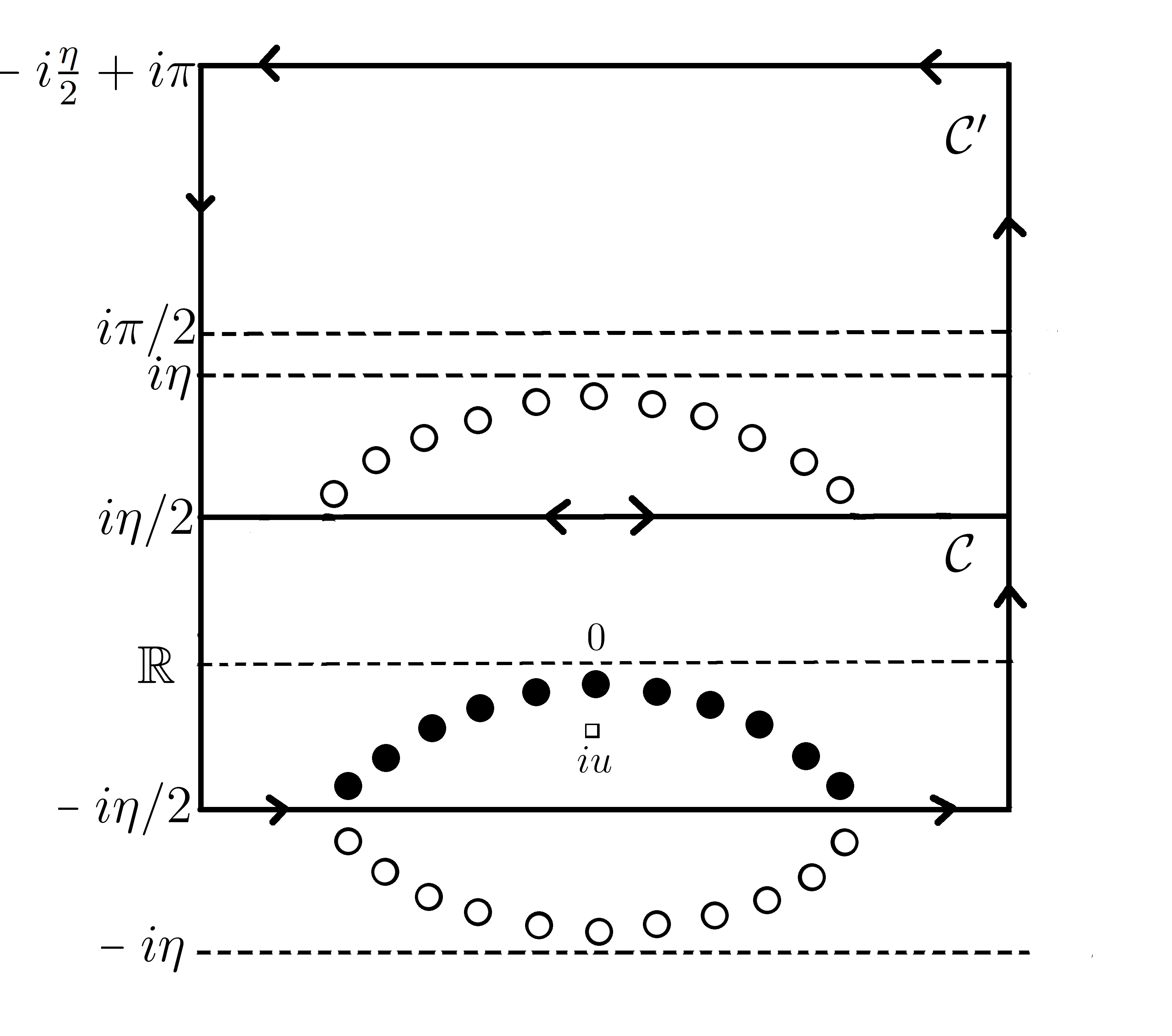
Figure 1: Typical distribution of Bethe roots ($\bullet$) and holes ($\circ$) in the strip $|\Im\lambda|<\eta\,,\ \eta\in[0,\pi/2)$ characterizing the largest eigenvalue of the QTM at low-temperatures. All the other roots and holes can be obtained using the $i\pi$ periodicity. The contour $\mathcal{C}$ surrounds all the Bethe roots and the pole of the auxiliary function $\mathfrak{a}(\lambda)$ at $iu$.

Let $\mathcal{C}$ be a rectangular contour with positive orientation, centered at the origin, extending to infinity, with the upper (lower) edges parallel to the real axis through $\pm i(\eta-\epsilon)/2,$ with $\epsilon\rightarrow 0$. It is important to note that this contour is independent of the Trotter number and the following considerations are valid for all $N$. Inside the contour, the function $1+\mathfrak{a}(\lambda)$ has $N/2$ zeros at the Bethe roots and a pole of order $N/2$ at $iu$, which means that $\log(1+\mathfrak{a}(\lambda))$ has no winding number around the contour allowing us to define ($\lambda$ is located outside of $\mathcal{C}$)

$$f(\lambda)\equiv\frac{1}{2\pi i}\int_{\mathcal{C}}\frac{d}{d\lambda}\left(\log\sinh(\lambda-\mu)\right)\log(1+\mathfrak{a}(\mu))d\mu=\frac{1}{2\pi i}\int_{\mathcal{C}}\log\sinh(\lambda-\mu)\frac{\mathfrak{a}^{\prime}(\mu)}{1+\mathfrak{a}(\mu)}d\mu\,.$$ (43)

For the evaluation of the r.h.s. of Eq. (43) we will use the following theorem:

Theorem 1.

WW Let $\mathcal{C}$ be a contour in the complex plane, and let $g(\lambda)$ be a function analytic and non-zero inside and on $\mathcal{C}$. Let $\phi(\lambda)$ be another function which is analytic inside and on $\mathcal{C}$ except at a finite number of points; let the zeros of $\phi(\lambda)$ in the interior of $\mathcal{C}$ be $a_{1},a_{2},\cdots$ and let their degrees of multiplicity be $r_{1},r_{2},\cdots$; and let its poles in the interior of $\mathcal{C}$ be $b_{1},b_{2},\cdots$ and let their degrees of multiplicity be $s_{1},s_{2},\cdots.$ Then

$$\frac{1}{2\pi i}\int_{\mathcal{C}}g(\lambda)\frac{\phi^{\prime}(\lambda)}{\phi(\lambda)}d\lambda=\sum_{i\in\mbox{zeros}}r_{i}g(a_{i})-\sum_{i\in\mbox{poles}}s_{i}g(b_{i})\,,$$

obtaining

$$f(\lambda)=\sum_{j=1}^{N/2}\log\sinh(\lambda-\lambda_{j})-\frac{N}{2}\log\sinh(\lambda-iu)=\log q(\lambda)-\log\phi_{-}(\lambda)-\frac{N}{2}\log\sin\eta\,.$$ (44)

Eq. (44) provides an integral representation for $q(\lambda)$ in terms of $\log(1+\mathfrak{a}(\lambda))$. Taking the logarithm in Eq. (42) and using (44) we can derive

$$\log\mathfrak{a}(\lambda)=-\beta h+\log\left(\frac{\phi_{+}(\lambda)}{\phi_{-}(\lambda)}\frac{\phi_{-}(\lambda+i\eta)}{\phi_{+}(\lambda+i\eta)}\right)+f(\lambda+i\eta)-f(\lambda-i\eta)\,,$$

which is a nonlinear integral equation of convolution type for the auxiliary function $\mathfrak{a}(\lambda),$ valid for all $N$. Using

$$\lim_{N\rightarrow\infty}\log\left(\frac{\phi_{+}(\lambda)}{\phi_{-}(\lambda)}\right)=-2J\beta\sinh(i\eta)\coth\lambda\,,$$ (45)

the Trotter limit, $N\rightarrow\infty,$ can be performed with the final result

$$\log\mathfrak{a}(\lambda)=-\beta h-\beta\frac{2J\sinh^{2}(i\eta)}{\sinh(\lambda+i\eta)\sinh\lambda}-\frac{1}{2\pi}\int_{\mathcal{C}}\frac{\sin(2\eta)}{\sinh(\lambda-\mu+i\eta)\sinh(\lambda-\mu-i\eta)}\log(1+\mathfrak{a}(\mu))d\mu\,.$$ (46)

Eq. (46) was obtained under the assumption that $\eta\in(0,\pi/2).$ It is also valid for $\eta\in(\pi/2,\pi)$ but in this case $\mathcal{C}$ is a rectangular contour centered at zero, extending to infinity, with the upper (lower) edges parallel to the real axis through $\pm i(\pi-\eta-\epsilon)/2$ with $\epsilon\rightarrow 0$.

IV.1.2 Integral expression for the largest eigenvalue

It remains to obtain an integral expression for the largest eigenvalue $\Lambda_{0}(\lambda)$ in terms of the auxiliary function $\mathfrak{a}(\lambda).$ Consider $\eta\in(0,\pi/2)$ for which the distribution of roots and holes is presented in Fig. 1. First, we note that Eq. (41) can be rewritten as

$$\Lambda_{0}(\lambda)=\frac{p(\lambda)}{\phi_{-}(\lambda-i\eta)\phi_{+}(\lambda+i\eta)q(\lambda)}\,,$$ (47)

with $p(\lambda)=\phi_{-}(\lambda)\phi_{+}(\lambda+i\eta)q(\lambda-i\eta)e^{\beta h/2}+\phi_{+}(\lambda)\phi_{-}(\lambda-i\eta)q(\lambda+i\eta)e^{-\beta h/2}.$ The function $p(\lambda)$ is quasi-periodic $p(\lambda+i\pi)=(-1)^{3N/2}p(\lambda)$ and $\lim_{\lambda\rightarrow\infty}p(\lambda)/(\sinh\lambda)^{3N/2}=(e^{\beta h/2}+e^{-\beta h/2})/(\sin\eta)^{N}.$ The zeros of the function $p(\lambda)$ in a strip of width $i\pi$ are the solutions of the equations $\mathfrak{a}(\lambda)=-1$ yielding

$$p(\lambda)=c\,\prod_{j=1}^{N/2}\sinh(\lambda-\lambda_{j})\prod_{j=1}^{N}\sinh(\lambda-\lambda_{j}^{(h)})\,,$$ (48)

where $\{\lambda_{j}\}_{j=1}^{N/2}$ and $\{\lambda_{j}^{(h)}\}_{j=1}^{N}$ are the Bethe roots and holes, respectively, and $c$ is a constant. Defining $q^{(h)}(\lambda)=\prod_{j=1}^{N}\sinh(\lambda-\lambda_{j}^{(h)})$ and using (48) to replace $p(\lambda)$ in Eq. (47) we obtain

$$\Lambda_{0}(\lambda)=c\,\frac{q^{(h)}(\lambda)}{\phi_{-}(\lambda-i\eta)\phi_{+}(\lambda+i\eta)}\,,$$ (49)

which provides an alternative expression for the largest eigenvalue in terms of the holes and not Bethe roots. Below, we will show how an integral representation of $\log q^{(h)}(\lambda)$ in terms of the auxiliary function $\mathfrak{a}(\lambda)$ can be calculated.

We consider a new rectangular contour with positive orientation $\mathcal{C}^{\prime}$ (see Fig. 1) extending to infinity, with the upper (lower) edges parallel to the real axis through $i(\eta-\epsilon)/2$ and $-i(\eta-\epsilon)/2+i\pi$ with $\epsilon\rightarrow 0$. The lower edge of the contour $\mathcal{C}^{\prime}$ at $i(\eta-\epsilon)/2$ coincides with the upper edge of $\mathcal{C}$ but has opposite orientation. Now we can prove the following identity

$$\int_{\mathcal{C}+\mathcal{C}^{\prime}}d(\lambda-\mu)\frac{\mathfrak{a}^{\prime}(\mu)}{1+\mathfrak{a}(\mu)}d\mu=0\,,\ \ \ \ d(\lambda-\mu)=\frac{d}{d\lambda}\log\sinh(\lambda-\mu)\,.$$ (50)

First, we notice that the contributions of the two contours parallel to the real axis through $i(\eta-\epsilon)/2$ cancel each other due to the opposite orientation. Then it can be easily verified using the definition of $\mathfrak{a}(\lambda)$ (42) that the functions appearing in (50) are all periodic of period $i\pi,$ which means that the upper and lower edges of $\mathcal{C}+\mathcal{C}^{\prime}$ do not contribute to the integral. Finally, the contributions of the sides parallel to the imaginary axis are also zero as it can be seen from

$$\lim_{\Re\mu\rightarrow\pm\infty}d(\lambda-\mu)=\mp 1\,,\ \ \ \frac{\mathfrak{a}^{\prime}(\mu)}{1+\mathfrak{a}(\mu)}=\frac{\mathfrak{a}^{\prime}(\mu)}{\mathfrak{a}\,(\mu)}\frac{1}{1+\mathfrak{a}^{-1}(\mu)}\,,\ \ \ \lim_{\Re\mu\rightarrow\pm\infty}\frac{1}{1+\mathfrak{a}^{-1}(\mu)}\rightarrow\frac{1}{1+e^{\beta h}}\,,\ \ \ \lim_{\Re\mu\rightarrow\pm\infty}\frac{\mathfrak{a}^{\prime}(\mu)}{\mathfrak{a}\,(\mu)}=0\,.$$

Consider $\lambda$ close to the real axis. Then making use of (50) we find

$$\frac{1}{2\pi i}\int_{\mathcal{C}}d(\lambda-\mu)\frac{\mathfrak{a}^{\prime}(\mu)}{1+\mathfrak{a}(\mu)}d\mu=-\frac{1}{2\pi i}\int_{\mathcal{C^{\prime}}}d(\lambda-\mu)\frac{\mathfrak{a}^{\prime}(\mu)}{1+\mathfrak{a}(\mu)}d\mu\,.$$ (51)

The r.h.s. of (51) can be calculated using Theorem 1 by taking into account that the function $1+\mathfrak{a}(\lambda)$ has inside the contour $\mathcal{C}^{\prime},$ $N$ zeros at the holes $\{\lambda_{j}^{(h)}\}_{j=1}^{N}$ or $\{\lambda_{j}^{(h)}\}_{j=1}^{N}+i\pi$, $N/2$ simple poles at $\{\lambda_{j}\}_{j=1}^{N/2}+i\eta$ and a pole of order $N/2$ at $-iu-i\eta+i\pi$ with the result

$$\frac{1}{2\pi i}\int_{\mathcal{C}}d(\lambda-\mu)\frac{\mathfrak{a}^{\prime}(\mu)}{1+\mathfrak{a}(\mu)}d\mu=-\left(\sum_{j=1}^{N}d(\lambda-\lambda_{j}^{(h)})-\sum_{j=1}^{N/2}d(\lambda-\lambda_{j}-i\eta)-\frac{N}{2}d(\lambda+iu+i\eta)\right)\,.$$ (52)

Using again Theorem 1 and the fact that the function $1+\mathfrak{a}(\lambda)$ has inside the contour $\mathcal{C},$ $N/2$ zeros at the Bethe roots $\{\lambda_{j}\}_{j=1}^{N/2}$ and a pole of order $N/2$ at $iu$ we find

$$\frac{1}{2\pi i}\int_{\mathcal{C}}d(\lambda-\mu-i\eta)\frac{\mathfrak{a}^{\prime}(\mu)}{1+\mathfrak{a}(\mu)}d\mu=\sum_{j=1}^{N/2}d(\lambda-\lambda_{j}-i\eta)-\frac{N}{2}d(\lambda-iu-i\eta)\,.$$ (53)

The integral representation for $\log q^{(h)}(\lambda)$ is obtained by taking the difference of Eqs. (52) and (53), integrating by parts, and then integrating w.r.t. $\lambda$ with the result

$$\frac{1}{2\pi i}\int_{\mathcal{C}}\left[d(\lambda-\mu)-d(\lambda-\mu-i\eta)\right]\log(1+\mathfrak{a}(\mu))d\mu=-\log q^{(h)}(\lambda)+\log\left(\phi_{+}(\lambda+i\eta)\phi_{-}(\lambda-i\eta)\right)+c\,,$$ (54)

where $c$ is a constant of integration. Making use of this integral representation in Eq. (49) the largest eigenvalue of the QTM can be written as

$$\log\Lambda_{0}(\lambda)=c+\frac{1}{2\pi i}\int_{\mathcal{C}}\frac{\sinh(i\eta)}{\sinh(\lambda-\mu-i\eta)\sinh(\lambda-\mu)}\log(1+\mathfrak{a}(\mu))d\mu\,.$$

The constant of integration is computed using the behavior of the involved functions at infinity. Performing the change of variables $z=\lambda-\mu$ in the integral, and using $\lim_{\lambda\rightarrow\infty}\log\Lambda_{0}(\lambda)=\log(e^{\beta h/2}+e^{-\beta h/2})$ and $\lim_{\lambda\rightarrow\infty}\log(1+\mathfrak{a}(\lambda))=\log(1+e^{-\beta h})$, we find that the constant of integration is $\beta h/2.$ The final result for the largest eigenvalue of the QTM evaluated at $0$ is

$$\log\Lambda_{0}(0)=\frac{\beta h}{2}+\frac{1}{2\pi}\int_{\mathcal{C}}\frac{\sin\eta}{\sinh(\mu+i\eta)\sinh(\mu)}\log(1+\mathfrak{a}(\mu))d\mu\,.$$ (55)

The integral expression (55), which was obtained for $\eta\in(0,\pi/2)$, is also valid for $\eta\in(\pi/2,\pi)$ but, as in the case of the NLIE for the auxiliary function (46), the contour $\mathcal{C}$ should be replaced by a similar rectangular contour with the upper (lower) edges parallel to the real axis through $\pm i(\pi-\eta-\epsilon)/2$ with $\epsilon\rightarrow 0$.

IV.1.3 Final form of the integral equations

The NLIE (46) and integral expression (55) are in fact correct for all temperatures K3 . This is due to the fact that, even at high temperatures, the Bethe roots are contained in the strip $|\Im\lambda|<(\eta-\epsilon)/2$ for $\eta\in(0,\pi/2)$ (or the strip $|\Im\lambda|<(\pi-\eta-\epsilon)/2$ for $\eta\in(\pi/2,\pi)$), which means that the reasoning of the previous sections is still valid, producing the same results. However, in order to obtain the thermodynamic properties and correlation lengths of the Bose gas we will be interested only in the low-temperature limit in which some simplifications of (46) and (55) appear.

Let us consider $\eta\in(\pi/2,\pi)$. In this case, the upper edge of the contour $\mathcal{C}$, which we will call $\mathcal{C}_{+}$, is a parallel line to the real axis through $i(\pi-\eta-\epsilon)/2$ (for the following discussion the presence of the $\epsilon$ term is irrelevant). Then for $\lambda\in\mathcal{C}_{+}\,,$ $\lambda=x+i(\pi-\eta)/2$ with $x$ real, the driving term on the r.h.s. of (46) is negative and equal to

$$-\beta h-\beta\frac{2J\sin^{2}\eta}{\cosh(x+i\eta/2)\cosh(x-i\eta/2)}\,,$$

which means that in the low-temperature limit $\beta\rightarrow\infty\,,$ $(h,J>0)$, the contribution of the upper part of the contour is negligible and we can restrict the free argument $\lambda$ and the integration variable to the lower part of the contour. We can shift this line to the line parallel to the real axis through $-i\eta/2$ without crossing any poles of the driving term obtaining

$$\log\mathfrak{a}(\lambda-i\eta/2)=-\beta h-\beta\frac{2J\sinh^{2}(i\eta)}{\sinh(\lambda+i\eta/2)\sinh(\lambda-i\eta/2)}-\frac{1}{2\pi}\int_{\mathbb{R}}\frac{\sin(2\eta)}{\sinh(\lambda-\mu+i\eta)\sinh(\lambda-\mu-i\eta)}\log(1+\mathfrak{a}(\mu-i\eta/2))d\mu\,.$$ (56)

Applying a similar reasoning to the integral expression of the largest eigenvalue (55), after the shift at $-i\eta/2$, we find

$$\log\Lambda_{0}(0)=\frac{\beta h}{2}+\frac{1}{2\pi}\int_{\mathbb{R}}\frac{\sin\eta}{\sinh(\mu+i\eta/2)\sinh(\mu-i\eta/2)}\log(1+\mathfrak{a}(\mu-i\eta/2))d\mu\,.$$ (57)

Let us introduce the function $\varepsilon(\lambda)$ satisfying $e^{-\varepsilon(\lambda)/T}=\mathfrak{a}(\lambda-i\eta/2)$ where $T=1/\beta$ is the temperature. Then noticing that the driving term in Eq. (56) is the magnon energy (17), and using (20) and (21), the NLIE for the auxiliary function and the integral expression for the largest eigenvalue at low-temperatures can be written as

$$\varepsilon(\lambda) =e_{0}(\lambda)+\frac{T}{2\pi}\int_{\mathbb{R}}K(\lambda-\mu)\log\left(1+e^{-\varepsilon(\mu)/T}\right)d\mu\,,$$ (58a)

$$\log\Lambda_{0}(0) =\frac{h}{2T}+\frac{1}{2\pi}\int_{\mathbb{R}}p_{0}^{\prime}(\lambda)\log\left(1+e^{-\varepsilon(\lambda)/T}\right)d\lambda\,.$$ (58b)

These equations are very similar to the Yang-Yang equation for the excitation energy and the grand-canonical potential of the Bose gas YY4 . Following SBGK , in Sec. VI we will show that the Yang-Yang thermodynamics can be obtained from Eqs. (58) if we perform the scaling limit presented in Sec.III.2. Even though Eqs. (58) were obtained for $\eta\in(\pi/2,\pi),$ they are also valid for $\eta\in(0,\pi/2),$ which can be proved by using appropriate contour manipulations. As these are beyond the scope of this paper, we confine ourselves to assuming the validity. This assumption will be verified in Sec. V where we will show that they reproduce the TLL/CFT predictions for the free energy and asymptotic behavior of the correlation functions.

IV.2 Integral equations for the next-largest eigenvalues in the $N/2$ sector

Computing the correlation lengths for the Green’s function $\langle\sigma_{z}^{(1)}\sigma_{z}^{(m+1)}\rangle_{T}$ requires the derivation of integral equations for the next-largest eigenvalues of the QTM in the $N/2$ sector. This means that, as in the case of the largest eigenvalue, we will have $N/2$ Bethe roots and $N$ holes. In the previous section we have derived the NLIE for the auxiliary function and the integral expression for the largest eigenvalue making use of the fact that the Bethe roots were located in a relevant strip (modulo the periodicity) of the complex plane which was independent of the Trotter number and temperature. In the case of the next-largest eigenvalues in the $N/2$ sector at low-temperatures, some of the Bethe roots are found outside of this strip and an equal number of holes are inside the strips. We will employ the same method used in Sec. IV.1 but modified in such a way that these Bethe roots and holes are properly taken into account. The calculations are presented in Appendix A. At low-temperatures, the next-largest eigenvalues of the QTM in the $N/2$ sector are given by

$$\log\Lambda^{(ph)}_{i}(0)=\frac{h}{2T}+i\sum_{j=1}^{r}p_{0}(\lambda^{+}_{j})-i\sum_{j=1}^{r}p_{0}(\lambda^{-}_{j})+\frac{1}{2\pi}\int_{\mathbb{R}}p_{0}^{\prime}(\lambda)\log\left(1+e^{-u_{i}(\lambda)/T}\right)d\lambda\,,$$ (59)

with the auxiliary functions $u_{i}(\lambda)$ satisfying the NLIEs

$$u_{i}(\lambda)=e_{0}(\lambda)-iT\sum_{j=1}^{r}\theta(\lambda-\lambda^{+}_{j})+iT\sum_{j=1}^{r}\theta(\lambda-\lambda^{-}_{j})+\frac{T}{2\pi}\int_{\mathbb{R}}K(\lambda-\mu)\log\left(1+e^{-u_{i}(\mu)/T}\right)d\mu\,.$$ (60)

The parameters $\{\lambda^{+}_{j}\}_{j=1}^{r}$ and $\{\lambda^{-}_{j}\}_{j=1}^{r},$ which belong to the upper, resp., lower half-plane are fixed by the constraint $1+e^{-u_{i}(\lambda^{\pm}_{j})/T}=0.$ In Eqs. (59) and (60), $r$ can take the values $1,2\cdots$. The subscript $i$ enumerates the sets of parameters $\{\lambda^{\pm}_{j}\}_{j=1}^{r}$ satisfying the constraint $1+e^{-u_{i}(\lambda^{\pm}_{j})/T}=0$.

IV.3 Integral equations for the next-largest eigenvalues in the $N/2-1$ sector

The next-largest eigenvalues in the $N/2-1$ sector are relevant for the computation of the correlation lengths of the Green’s function $\langle\sigma_{+}^{(1)}\sigma_{-}^{(m+1)}\rangle_{T}.$ The eigenvalues in this sector are characterized by $p=N/2-1$ in Eqs. (36) and (37). Some of the features encountered in the study of the largest and $N/2$ sector eigenvalues are also present in this case.

At low-temperatures, the next-largest eigenvalue in this sector has $N/2-1$ Bethe roots and, possibly, a hole in a certain strip of the complex plane. Eigenvalues with decreasing magnitude are obtained by moving pairs of Bethe roots/holes outside/inside the strip. This means that it is sufficient to obtain integral equations for the cases with one hole or no hole inside the strip, the equations for the other eigenvalues are obtained by adding extra driving terms of the type encountered in Eqs. (59) and (60). The necessary calculations are presented in Appendix B. We distinguish two cases. For $\lambda_{0}$ in the upper half plane, the next-largest eigenvalues in the $N/2-1$ sector at low-temperatures have the integral representation

$$\log\Lambda^{(s)}_{i}(0)=\frac{h}{2T}-i\pi+ip_{0}(\lambda_{0})+i\sum_{j=1}^{r}p_{0}(\lambda^{+}_{j})-i\sum_{j=1}^{r}p_{0}(\lambda^{-}_{j})+\frac{1}{2\pi}\int_{\mathbb{R}}p_{0}^{\prime}(\lambda)\log\left(1+e^{-v_{i}(\lambda)/T}\right)d\lambda\,,$$ (61)

with the auxiliary functions $v_{i}(\lambda)$ satisfying the NLIEs

$$v_{i}(\lambda)=e_{0}(\lambda)\pm i\pi T-iT\theta(\lambda-\lambda_{0})-iT\sum_{j=1}^{r}\theta(\lambda-\lambda^{+}_{j})+iT\sum_{j=1}^{r}\theta(\lambda-\lambda^{-}_{j})+\frac{T}{2\pi}\int_{\mathbb{R}}K(\lambda-\mu)\log\left(1+e^{-v_{i}(\mu)/T}\right)d\mu\,.$$ (62)

The $2r+1$ parameters $\lambda_{0}\,,\{\lambda^{+}_{j}\}_{j=1}^{r}$ and $\{\lambda_{j}^{-}\}_{j=1}^{r}$ which belong to the upper, resp., lower half-plane are fixed by the constraints $1+e^{-v_{i}(\lambda_{0})/T}=0\,,1+e^{-v_{i}(\lambda^{\pm}_{j})/T}=0.$ On the r.h.s. of Eq. (62) the plus (minus) sign in front of the $i\pi T$ term is considered when $\lambda_{0}$ is in the first (second) quadrant of the complex plane $\Re\lambda_{0}\geq 0\,,\Im\lambda_{0}\geq 0$ ($\Re\lambda_{0}<0\,,\Im\lambda_{0}\geq 0$). For $\lambda_{0}$ in the lower half-plane Eqs. (61) and (62) remain valid but the integration contour now is the real axis with an indentation such that $\lambda_{0}$ is above the contour. Also, the plus (minus) sign in front of the $i\pi T$ term of (62) is considered when $\lambda_{0}$ is in the fourth (third) quadrant of the complex plane $\Re\lambda_{0}\geq 0\,,\Im\lambda_{0}\leq 0$ ($\Re\lambda_{0}<0\,,\Im\lambda_{0}\leq 0$). In this case $\lambda_{0}$, which satisfies $1+e^{-v_{i}(\lambda_{0})/T}=0$, is the closest solution to the real axis in the lower half-plane.

V Comparison with the TLL/CFT predictions

In Sec. IV.1.3 we have derived an integral expression (58), for the largest eigenvalue of the QTM in terms of an auxiliary function which obeys a NLIE very similar to the Yang-Yang equation (8). Eq.  (58) and the similar integral representations for the next-largest eigenvalues (59) and (61), are valid only at low-temperatures and, in the course of the derivation, we have made some assumptions which were not fully justified for some values of the anisotropy. Here, we will show that our results are in perfect agreement with the predictions of the Tomonaga-Luttinger liquid H1 ; H2 and Conformal Field Theory BPZ ; C1 ; VW ; C2 ; BCN ; A ; BIK , confirming the validity of our assumptions.

V.1 Low-temperature behavior of the free energy

At low-temperatures CFT predicts A that the free energy per lattice site scales like

$$f(h,T)=\epsilon_{0}(h)-\frac{\pi T^{2}c}{6v_{F}}+O(T^{3})\,,\ \ \ \epsilon_{0}(h)=-\frac{h}{2}+\int_{-q}^{q}e_{0}(\lambda)\rho(\lambda)d\lambda\,,$$ (63)

where $\epsilon_{0}(h)$ is the density of the ground state energy, $c$ is the conformal charge, (not to be confused with the coupling constant of the Bose gas), which is equal to one in the case of the XXZ spin chain, and $v_{F}$ is the Fermi velocity defined as

$$v_{F}=\frac{\varepsilon_{0}^{\prime}(q)}{2\pi\rho(q)}\,,$$ (64)

with $\varepsilon_{0}^{\prime}(q)$ the derivative of the dressed energy (22) evaluated at the Fermi boundary $q$.

Let us show that the free energy per lattice site obtained from Eq. (58b), via $f(h,T)=-T\log\Lambda_{0}(0)$, satisfies (63). Performing an analysis similar to the one in Appendix A of YY4 or Chap. I of KBI it can be shown that for $\eta\in(0,\pi)$ and $h<h_{c}=8J\cos^{2}(\eta/2)$, the NLIE (58a) for the auxiliary function $\varepsilon(\lambda)$ has two zeros on the real axis which we will denote by $\pm q(T).$ Also $\varepsilon(\lambda)$ is negative on $\left(-q(T),q(T)\right)$ and positive outside of this interval. Let us denote $\lim_{T\rightarrow 0}q(T)=\tilde{q}$ and $\lim_{T\rightarrow 0}\varepsilon(\lambda)=\tilde{\varepsilon}_{0}(\lambda)$. Then using

$$\lim_{T\rightarrow 0}T\log\left(1+e^{-\varepsilon(\lambda)/T}\right)=\left\{\begin{array}[]{ccl}-\tilde{\varepsilon}_{0}(\lambda)&&\lambda\in(-\tilde{q},\tilde{q})\,,\\ 0&&\lambda\in(-\infty,-\tilde{q})\cup(\tilde{q},+\infty)\,,\end{array}\right.$$ (65)

we find that in the low-temperature limit the NLIE (58a) transforms in the linear equation for the dressed energy (22). The equation for the dressed energy has a unique solution for $\eta\in(0,\pi)$ which means that $\lim_{T\rightarrow 0}\varepsilon(\lambda)=\varepsilon_{0}(\lambda)$ and $\lim_{T\rightarrow 0}q(T)=q$. In order to show that Eq. (58b) gives the correct free energy satisfying (63) we need a more accurate estimation of integrals containing the factor $\log\left(1+e^{-\varepsilon(\lambda)/T}\right)$. In the following we are going to assume that for low temperatures the auxiliary function has the expansion JM ; MN ; S1

$$\varepsilon(\lambda)=\varepsilon_{0}(\lambda)+\varepsilon_{1}(\lambda)T+\varepsilon_{2}(\lambda)T^{2}+O(T^{3})\,.$$ (66)

Then it can be shown (see Appendix A of KMS2 or KKK2 ) that, for any function $f(\lambda)$, bounded on the real axis and differentiable in the vicinity of $\pm q$ we have :

$$\lim_{T\rightarrow 0}T\int_{\mathbb{R}}f(\lambda)\log\left(1+e^{-\varepsilon(\lambda)/T}\right)\,d\lambda=-\int_{-q}^{q}f(\lambda)\varepsilon(\lambda)d\lambda$$

$$\ \ \ \ \ \ \ \ \ \ \ \ \ \ \ \ \ \ \ \ \ \ \ \ \ \ \ \ \ \ \ +\frac{T^{2}\pi^{2}}{6\varepsilon_{0}^{\prime}(q)}(f(q)+f(-q))+\frac{T^{2}\varepsilon_{1}^{2}(q)f(q)}{2\varepsilon_{0}^{\prime}(q)}+\frac{T^{2}\varepsilon_{1}^{2}(-q)f(-q)}{2\varepsilon_{0}^{\prime}(q)}+O(T^{3})\,.$$ (67)

We should mention that a more compact, but maybe not as transparent, method of investigating the low-temperature limit of the QTM spectrum was employed in KSc . All the results derived here and in the following sections can also be obtained utilizing the results of the aforementioned paper. Using (V.1) and substituting (66) in the equation for the auxiliary function (58a) we obtain

$$\sum_{k=0}^{2}T^{k}\varepsilon_{k}(\lambda)+\frac{1}{2\pi}\sum_{k=0}^{2}T^{k}\int_{-q}^{q}K(\lambda-\mu)\varepsilon_{k}(\mu)\,d\mu=e_{0}(\lambda)\,$$

$$\ \ \ \ \ \ \ \ \ \ \ \ \ \ \ \ -\frac{\pi T^{2}}{12\varepsilon_{0}^{\prime}(q)}(K(\lambda-q)+K(\lambda+q))-\frac{T^{2}\varepsilon_{1}^{2}(q)}{4\pi\varepsilon_{0}^{\prime}(q)}K(\lambda-q)-\frac{T^{2}\varepsilon_{1}^{2}(-q)}{4\pi\varepsilon_{0}^{\prime}(q)}K(\lambda+q)+O(T^{3})\,.$$

Equating terms of the same order in temperature we find

$$\varepsilon_{1}(\lambda)=0\,,\ \ \ \ \varepsilon_{2}(\lambda)=\frac{\pi^{2}}{6\varepsilon_{0}^{\prime}(q)}(R(\lambda,q)+R(\lambda,-q))\,,$$ (68)

with the resolvent $R(\lambda,\mu)$ defined in (24). The low-temperature expansion of the free energy per lattice site is calculated using the asymptotic formula (V.1) in Eq. (58b) with the result

$$f(h,T)=-\frac{h}{2}+\frac{1}{2\pi}\int_{-q}^{q}p_{0}^{\prime}(\lambda)(\varepsilon_{0}(\lambda)+\varepsilon_{2}(\lambda)T^{2})\,d\lambda-\frac{\pi T^{2}}{12\varepsilon_{0}^{\prime}(q)}p_{0}^{\prime}(q)+O(T^{3})\,,$$ (69)

where we have used the fact that $p_{0}^{\prime}(\lambda)$ is even, $p_{0}^{\prime}(-q)=p_{0}^{\prime}(q)$. Using Eq. (68) and the identity

$$\int_{-q}^{q}p_{0}^{\prime}(\lambda)R(\lambda,\pm q)\,d\lambda=p_{0}^{\prime}(q)-2\pi\rho(q)\,,$$ (70)

(for a proof, see Appendix C), (69) takes the form

$$f(h,T)=-\frac{h}{2}+\frac{1}{2\pi}\int_{-q}^{q}p_{0}^{\prime}(\lambda)\varepsilon_{0}(\lambda)\,d\lambda-\frac{\pi T^{2}}{6}\frac{2\pi\rho(q)}{\varepsilon_{0}^{\prime}(q)}+O(T^{3})\,.$$ (71)

Using the identity (123) and the definition of the Fermi velocity (64), it is easy to see that this expression is identical with (63).

V.2 Low-temperature asymptotic behavior of the longitudinal correlation

The Tomonaga-Luttinger liquid theory and CFT predict the following asymptotic behavior of the longitudinal correlation function at low-temperatures (we consider only the leading-order of the oscillatory terms) BIK

$$\langle\sigma^{(1)}_{z}\sigma^{(m+1)}_{z}\rangle_{T}=\langle\sigma^{(1)}_{z}\rangle^{2}_{T}-\frac{(T\mathcal{Z}/v_{F})^{2}}{2\sinh^{2}(\pi Tm/v_{F})}+\sum_{l\in\mathbb{Z}^{*}}A_{l}\ e^{2imlk_{F}}\left(\frac{\pi T/v_{F}}{\sinh(\pi Tm/v_{F})}\right)^{2l^{2}\mathcal{Z}^{2}}\,,\ \ \ \ \ m\rightarrow\infty\,,$$ (72)

with the Fermi momentum defined by $k_{F}=\pi D$ and $A_{l}$ are coefficients that do not depend on $T$. The analysis of the QTM spectrum EPAPS shows that the asymptotic behavior of the correlation function can be expressed as

$$\langle\sigma^{(1)}_{z}\sigma^{(m+1)}_{z}\rangle_{T}=const+\sum_{i}\tilde{A}_{i}\,e^{-\frac{m}{\xi^{(d)}[u_{i}]}}\,,\ \ \ \ \ m\rightarrow\infty\,,$$ (73)

where the sum is over all the correlation lengths, $1/\xi^{(d)}[u_{i}]=\log(\Lambda_{0}(0)/\Lambda^{(i)}_{ph}(0))$, determined as the ratio of the largest and next-largest eigenvalues in the $N/2$ sector. Using (58b) and (59) we obtain the following explicit expression for the correlation lengths

$$\frac{1}{\xi^{(d)}[u_{i}]}=-\frac{1}{2\pi}\int_{\mathbb{R}}p_{0}^{\prime}(\lambda)\log\left(\frac{1+e^{-u_{i}(\lambda)/T}}{1+\,e^{-\varepsilon(\lambda)/T}}\right)\,d\lambda-i\sum_{j=1}^{r}p_{0}(\lambda^{+}_{j})+i\sum_{j=1}^{r}p_{0}(\lambda^{-}_{j})\,,$$ (74)

where the functions $\varepsilon(\lambda)$ and $u_{i}(\lambda)$ satisfy Eqs. (58a) and (60). In the rest of this section we will show that (73) is equivalent to (72) in the conformal limit.

The analysis of the correlation lengths (74) in the limit $T\rightarrow 0$ is very similar to the one performed by Kozlowski, Maillet and Slavnov for the correlation lengths of the Bose gas, and, for this reason, we are going to use some of the notations and terminology employed in KMS2 . In the following we are going to discard the subscript $i$ for the auxiliary function $u_{i}(\lambda)$. We are considering an arbitrary auxiliary function $u(\lambda)$ satisfying Eq. (60), with $2r$ parameters $\{\lambda^{+}_{j}\}_{j=1}^{r}$, $\{\lambda^{-}_{j}\}_{j=1}^{r}$, located in the upper (lower) half-plane, which also satisfy the constraint $1+e^{-u(\{\lambda^{\pm}_{j}\})/T}=0$. The first observation that we are going to make is that $\lim_{T\rightarrow 0}u(\lambda)=\varepsilon_{0}(\lambda)$. In analogy with the case of the auxiliary function $\varepsilon(\lambda)$ we expect that all the solutions of the equation $1+e^{-u(\lambda)/T}=0$ will collapse at $\pm q$ in the limit $T\rightarrow 0$. We will say that the solutions that collapse at $q$ $(-q)$ belong to the right (left) series. If we assume that $u(\lambda)$ has the expansion

$$u(\lambda)=\varepsilon_{0}(\lambda)+u_{1}(\lambda)T+u_{2}(\lambda)T^{2}+O(T^{3})\,,$$ (75)

then a formula similar to (V.1) can be derived as in KMS2

$$\lim_{T\rightarrow 0}T\int_{\mathbb{R}}f(\lambda)\log\left(1+e^{-u(\lambda)/T}\right)\,d\lambda=-\int_{-q}^{q}f(\lambda)u(\lambda)d\lambda$$

$$\ \ \ \ \ \ \ \ \ \ \ \ \ \ \ \ \ \ \ \ \ \ \ \ \ \ \ \ \ \ \ +\frac{T^{2}\pi^{2}}{6\varepsilon_{0}^{\prime}(q)}(f(q)+f(-q))+\frac{T^{2}u_{1}^{2}(q)f(q)}{2\varepsilon_{0}^{\prime}(q)}+\frac{T^{2}u_{1}^{2}(-q)f(-q)}{2\varepsilon_{0}^{\prime}(q)}+O(T^{3})\,.$$ (76)

We are going to consider that the roots $\{\lambda^{\pm}\}$ are distributed in the following manner: $r_{p}^{+}$ roots $\lambda^{+}$ and $r_{h}^{+}$ roots $\lambda^{-}$ belonging to the right series (collapse at $q$); $r_{p}^{-}$ roots $\lambda^{+}$ and $r_{h}^{-}$ roots $\lambda^{-}$ belonging to the left series (collapsing at $-q$), where $r_{p}^{\pm}$ and $r_{h}^{\pm}$ satisfy the constraints

$$r_{p}^{+}+r_{p}^{-}=r_{h}^{+}+r_{h}^{-}=r\,,\ \ \ \ \ \ r_{p}^{+}-r_{h}^{+}=r_{h}^{-}-r_{p}^{-}=l\,,$$

with $l$ integer, satisfying $-r\leq l\leq r$. More explicitly, at sufficiently low temperatures we have

$$\{\lambda^{+}_{j}\}_{j=1}^{r} =\{q+iT\alpha_{k}^{+}\}_{k=1}^{r_{p}^{+}}\cup\{-q+iT\alpha_{k}^{-}\}_{k=1}^{r_{p}^{-}}\,,\ \ \ \ \Re(\alpha_{k}^{\pm})>0\,,$$ (77a)

$$\{\lambda^{-}_{j}\}_{j=1}^{r} =\{q-iT\,\beta_{k}^{+}\}_{k=1}^{r_{h}^{+}}\cup\{-q-iT\,\beta_{k}^{-}\}_{k=1}^{r_{h}^{-}}\,,\ \ \ \ \Re(\beta_{k}^{\pm})>0\,,$$ (77b)

where $\alpha_{k}^{\pm}$ and $\beta_{k}^{\pm}$ satisfy $1+e^{-u(\pm q+iT\alpha_{k}^{\pm})/T}=1+e^{-u(\pm q-iT\beta_{k}^{\pm})/T}=0\,.$ The leading Taylor coefficients can be parameterized by a set of integers, $p_{k}^{\pm}$ and $s_{k}^{\pm}$ via

$$u(\pm q+iT\alpha_{k}^{\pm})=\pm 2\pi iT(p_{k}^{\pm}-\frac{1}{2})\,,\ \ \ \ \ \ \ u(\pm q-iT\beta_{k}^{\pm})=\mp 2\pi iT(s_{k}^{\pm}-\frac{1}{2})\,.$$

Using the expansion (75), $\varepsilon(\pm q)=0\,$ and $\varepsilon_{0}^{\prime}(-q)=-\varepsilon_{0}^{\prime}(q)$ we find

$$\alpha_{k}^{\pm}=\frac{2\pi}{\varepsilon_{0}^{\prime}(q)}\left(p_{k}^{\pm}-\frac{1}{2}\right)\pm i\frac{u_{1}(\pm q)}{\varepsilon_{0}^{\prime}(q)}\,,\ \ \ \ \ \ \beta_{k}^{\pm}=\frac{2\pi}{\varepsilon_{0}^{\prime}(q)}\left(s_{k}^{\pm}-\frac{1}{2}\right)\mp i\frac{u_{1}(\pm q)}{\varepsilon_{0}^{\prime}(q)}\,.$$ (78)

Substituting the parametrization (77) in Eq. (60) and expanding the driving terms up to the second order in $T$ we find

$$u(\lambda)=e_{0}(\lambda)+\frac{T}{2\pi}\int_{\mathbb{R}}K(\lambda-\mu)\log\left(1+e^{-u(\lambda)/T}\right)\,d\mu+g_{1}(\lambda)T+g_{2}(\lambda)T^{2}+O(T^{3})\,,$$ (79)

with

$$g_{1}(\lambda)=-il(\theta(\lambda-q)-\theta(\lambda+q))\,,$$

and

$$g_{2}(\lambda)=-K(\lambda-q)\left(\sum_{k=1}^{r_{p}^{+}}\alpha_{k}^{+}+\sum_{k=1}^{r_{h}^{+}}\beta_{k}^{+}\right)-K(\lambda+q)\left(\sum_{k=1}^{r_{p}^{-}}\alpha_{k}^{-}+\sum_{k=1}^{r_{h}^{-}}\beta_{k}^{-}\right)\,.$$

We can now use (V.2) in (79) obtaining a system of equations for the unknown functions $u_{1}(\lambda)$ and $u_{2}(\lambda)$. For $u_{1}(\lambda)$ it reads

$$u_{1}(\lambda)+\frac{1}{2\pi}\int_{-q}^{q}K(\lambda-\mu)\,u_{1}(\mu)\,d\mu=-il(\theta(\lambda-q)-\theta(\lambda+q))\,.$$

Comparison with the integral equation for the dressed phase (25) shows that $u_{1}(\lambda)=-2\pi il(F(\lambda|q)-F(\lambda|-q))$. Using the first identity in (26) we can obtain an expression in terms of the dressed charge $u_{1}(\lambda)=2\pi il(1-Z(\lambda)).$ The equation for $u_{2}(\lambda)$ is

$$u_{2}(\lambda)+\frac{1}{2\pi}\int_{-q}^{q}K(\lambda-\mu)\,u_{2}(\mu)\,d\mu=g_{2}(\lambda)+K(\lambda-q)\left(\frac{\pi}{12\varepsilon_{0}^{\prime}(q)}+\frac{u_{1}^{2}(q)}{4\pi\varepsilon_{0}^{\prime}(q)}\right)+K(\lambda+q)\left(\frac{\pi}{12\varepsilon_{0}^{\prime}(q)}+\frac{u_{1}^{2}(-q)}{4\pi\varepsilon_{0}^{\prime}(q)}\right)\,,$$

with the solution

$$u_{2}(\lambda)=-R(\lambda,q)\left[\sum_{k=1}^{r_{p}^{+}}\alpha_{k}^{+}+\sum_{k=1}^{r_{h}^{+}}\beta_{k}^{+}-\frac{1}{2\varepsilon_{0}^{\prime}(q)}\left(\frac{\pi^{2}}{3}+u_{1}^{2}(q)\right)\right]-R(\lambda,-q)\left[\sum_{k=1}^{r_{p}^{-}}\alpha_{k}^{-}+\sum_{k=1}^{r_{h}^{-}}\beta_{k}^{-}-\frac{1}{2\varepsilon_{0}^{\prime}(q)}\left(\frac{\pi^{2}}{3}+u_{1}^{2}(-q)\right)\right]\,.$$

Using (V.1) and (V.2) in (74) and expanding the $p_{0}(\lambda^{\pm})$ terms up to the first order in $T$ we obtain

$$\frac{1}{\xi^{(d)}[u]}=-2ilk_{F}-T\frac{u_{1}^{2}(q)\rho(q)}{\varepsilon_{0}^{\prime}(q)}+2\pi T\rho(q)\left(\sum_{k=1}^{r_{p}^{+}}\alpha_{k}^{+}+\sum_{k=1}^{r_{p}^{-}}\alpha_{k}^{-}+\sum_{k=1}^{r_{h}^{+}}\beta_{k}^{+}+\sum_{k=1}^{r_{h}^{-}}\beta_{k}^{-}\right)+O(T^{2})\,.$$ (80)

In deriving (80) we have used also the identity $\int_{-q}^{q}p_{0}^{\prime}(\lambda)Z(\lambda)\,d\lambda=\int_{-q}^{q}\rho(\lambda)\,d\lambda$ and (121). Finally, using (78) we find

$$\frac{1}{\xi^{(d)}[u]}=-2ilk_{F}+\frac{2\pi T}{v_{F}}\left(l^{2}\mathcal{Z}^{2}-l^{2}-r+\sum_{k=1}^{r_{p}^{+}}p_{k}^{+}+\sum_{k=1}^{r_{p}^{-}}p_{k}^{-}+\sum_{k=1}^{r_{h}^{+}}s_{k}^{+}+\sum_{k=1}^{r_{h}^{-}}s_{k}^{-}\right)+O(T^{2})\,.$$ (81)

The second term in the expansion (72) is obtained for $r=1,l=0$ and $p_{1}^{+}=p_{1}^{-}=1$ (or $s_{1}^{+}=s^{-}_{1}=1$). The next leading terms are obtained for $r=l\,,l=1,2,\cdots$ and the integers $p^{+}_{k}$ and $s^{-}_{k}$ (or $p^{-}_{k}$ and $s^{+}_{k}$) taking values from $1$ to $l$.

There is, however, one caveat. If we assume $\Re(\alpha_{k}^{\pm})>0\,,\Re(\beta_{k}^{\pm})>0$, then, (78) together with $u_{1}(\pm q)=2\pi il(1-\mathcal{Z})$ impose some constraints on the allowed values of $p^{\pm}_{k}$ and $s^{\pm}_{k}$. A relatively straightforward analysis shows that for $\eta\in(\pi/2,\pi)\,,(\mathcal{Z}>1)$, which is the region most interesting for us, the allowed values for $p^{\pm}_{k}$ and $s^{\pm}_{k}$ contain $\{1,2,\cdots\}$. For $\eta\in(0,\pi/2)$ we have $1/\sqrt{2}<\mathcal{Z}<1$. In this case, for $\mathcal{Z}$ close to $1/\sqrt{2}$, the integers $p_{k}^{\pm}$ and $s_{k}^{\pm}$ can take the values $\{1,2,\cdots\}$ only for $l=0,\pm 1$. For $\mathcal{Z}\rightarrow 1$ the value of $l$ for which the allowed values of $p_{k}^{\pm}$ and $s_{k}^{\pm}$ contain $\{1,2,\cdots\}$ increases. This means that under the aforementioned assumptions, in the worst case scenario, our equations can reproduce only the $l=0,\pm 1$ terms of the CFT expansion.

V.3 Low-temperature asymptotic behavior of the transversal correlation

In the case of the transversal correlation TLL and CFT predict the following asymptotic behavior at low-temperatures BIK

$$\langle\sigma^{(1)}_{+}\sigma^{(m+1)}_{-}\rangle_{T}=\sum_{l\in\mathbb{Z}}B_{l}\ e^{2imlk_{F}}\left(\frac{\pi T/v_{F}}{\sinh(\pi Tm/v_{F})}\right)^{\frac{1}{2\mathcal{Z}^{2}}+2l^{2}\mathcal{Z}^{2}}\,,\ \ \ \ \ m\rightarrow\infty\,,$$ (82)

with $B_{l}$ coefficients that do not depend on $T$. The analysis of the correlation functions in the framework of the QTM EPAPS showed that

$$\langle\sigma^{(1)}_{+}\sigma^{(m+1)}_{-}\rangle_{T}=\sum_{i}\tilde{B}_{i}\,e^{-\frac{m}{\xi^{(s)}[v_{i}]}}\,,\ \ \ \ \ m\rightarrow\infty\,,$$ (83)

where the sum is over all the correlation lengths $1/\xi^{(s)}[v_{i}]=\log(\Lambda_{0}(0)/\Lambda^{(i)}_{s}(0))$, determined as the ratio of the largest and next-largest eigenvalues in the $N/2-1$ sector. Using (58b) and (61) we obtain the following explicit expression for the correlation lengths (we neglect the $i\pi$ term which produces an $(-1)^{m}$ factor)

$$\frac{1}{\xi^{(s)}[v_{i}]}=-\frac{1}{2\pi}\int_{\mathbb{R}}p_{0}^{\prime}(\lambda)\log\left(\frac{1+e^{-v_{i}(\lambda)/T}}{1+\,e^{-\varepsilon(\lambda)/T}}\right)\,d\lambda-ip_{0}(\lambda_{0})-i\sum_{j=1}^{r}p_{0}(\lambda^{+}_{j})+i\sum_{j=1}^{r}p_{0}(\lambda^{-}_{j})\,,$$ (84)

where $\lambda_{0}$ is in the upper half-plane and the functions $\varepsilon(\lambda)$ and $v_{i}(\lambda)$ satisfy Eqs. (58a) and (62). For $\lambda_{0}$ in the lower half-plane the integration contour is the real axis with an indentation such that $\lambda_{0}$ is above the contour.

First, we will consider the case with $\lambda_{0}$ in the upper half-plane. It is sufficient to consider the conformal limit of the following correlation length

$$\frac{1}{\xi^{(s)}[v]}=-\frac{1}{2\pi}\int_{\mathbb{R}}p_{0}^{\prime}(\lambda)\log\left(\frac{1+e^{-v(\lambda)/T}}{1+\,e^{-\varepsilon(\lambda)/T}}\right)\,d\lambda-ip_{0}(\lambda_{0})\,,$$ (85)

with $v(\lambda)$ satisfying the equation (62) with $r=0$. The behavior of the correlation length (84) will be obtained by summing the contributions of (85) and (74) derived in the previous section. We notice that $\lim_{T\rightarrow 0}v(\lambda)=\varepsilon_{0}(\lambda),$ therefore, we are going to consider the following expansion

$$v(\lambda)=\varepsilon_{0}(\lambda)+v_{1}(\lambda)T+v_{2}(\lambda)T^{2}+O(T^{3})\,,$$ (86)

with $v_{1}(\lambda)$ and $v_{2}(\lambda)$ unknown functions. Also (V.2) is still valid if we replace $u(\lambda)$ with $v(\lambda)$. We are going to consider that $\lambda_{0}$ is located in the first quadrant (this means that we are going to have a plus sign in front of the $i\pi T$ term in Eq. (62)). The same result is obtained if we consider $\lambda_{0}$ in the second quadrant. Then at sufficiently low-temperatures we have

$$\lambda_{0}=q+i\alpha_{0}^{+}T\,,\ \ \ \alpha_{0}^{+}=\frac{2\pi}{\varepsilon_{0}^{\prime}(q)}\left(p_{0}^{+}-\frac{1}{2}\right)+i\frac{v_{1}(q)}{\varepsilon_{0}^{\prime}(q)}\,,$$ (87)

with $p_{0}^{+}$ an integer parameterizing the leading Taylor coefficient $\alpha_{0}^{+}.$ Using this parametrization in Eq. (62), and expanding to the second order in $T$ we find

$$v(\lambda)=e_{0}(\lambda)+\frac{T}{2\pi}\int_{\mathbb{R}}K(\lambda-\mu)\log\left(1+e^{-v(\mu)/T}\right)\,d\mu+[i\pi-i\theta(\lambda-q)]T-K(\lambda-q)\alpha_{0}^{+}T^{2}+O(T^{3})\,,$$ (88)

The integral equations satisfied by $v_{1}(\lambda)$ and $v_{2}(\lambda)$ are obtained by substituting (V.2), modified for the $v(\lambda)$ function, in (88). For $v_{1}(\lambda)$ it reads

$$v_{1}(\lambda)+\frac{1}{2\pi}\int_{-q}^{q}K(\lambda-\mu)\,v_{1}(\mu)\,d\mu=i\pi-i\theta(\lambda-q)\,.$$

Comparison with the integral equation for the dressed phase (25) and dressed charge (23) shows that $v_{1}(\lambda)=i\pi Z(\lambda)-2i\pi F(\lambda|q))$. Using the first identity in (26) the solution to this equation can be rewritten as $v_{1}(\lambda)=i\pi(1-F(\lambda|q)-F(\lambda|-q)).$ The equation for $v_{2}(\lambda)$ is

$$v_{2}(\lambda)+\frac{1}{2\pi}\int_{-q}^{q}K(\lambda-\mu)\,v_{2}(\mu)\,d\mu=K(\lambda-q)\left(-\alpha_{0}^{+}+\frac{\pi}{12\varepsilon_{0}^{\prime}(q)}+\frac{v_{1}^{2}(q)}{4\pi\varepsilon_{0}^{\prime}(q)}\right)+K(\lambda+q)\left(\frac{\pi}{12\varepsilon_{0}^{\prime}(q)}+\frac{v_{1}^{2}(-q)}{4\pi\varepsilon_{0}^{\prime}(q)}\right)\,,$$

with the solution

$$v_{2}(\lambda)=-R(\lambda,q)\left[-2\pi\alpha_{0}^{+}-\frac{1}{2\varepsilon_{0}^{\prime}(q)}\left(\frac{\pi^{2}}{3}+v_{1}^{2}(q)\right)\right]-R(\lambda,-q)\left[-\frac{1}{2\varepsilon_{0}^{\prime}(q)}\left(\frac{\pi^{2}}{3}+v_{1}^{2}(-q)\right)\right]\,.$$

Using (V.1) and (V.2) in (85) and expanding the $p_{0}(\lambda^{+}_{0})$ term up to the first order in $T$ we obtain

$$\frac{1}{\xi^{(s)}[v]}=2\pi T\rho(q)\left(\alpha_{0}^{+}-\frac{v_{1}^{2}(q)}{4\pi\varepsilon_{0}^{\prime}(q)}-\frac{v_{1}^{2}(-q)}{4\pi\varepsilon_{0}^{\prime}(q)}\right)+O(T^{2})\,.$$ (89)

In deriving (89) we have also used the fact that $F(\lambda|q)+F(\lambda|-q)$ is an odd function of $\lambda,$ ($F(-\lambda|-\mu)=-F(\lambda|\mu)$) and (121). The final result follows from (87) and the use of the second identity in (26)

$$\frac{1}{\xi^{(s)}[v]}=\frac{2\pi T}{v_{F}}\left(\frac{1}{4\mathcal{Z}^{2}}+p_{0}^{+}-1\right)+O(T^{2})\,.$$ (90)

The case with $\lambda_{0}$ in the lower half-plane can be treated along similar lines if we notice that (V.2) remains valid even if on the l.h.s we have an integral over a modified contour. Considering $\lambda_{0}$ in the fourth quadrant then (87) is still valid but, in this case, $\Re\alpha_{0}^{+}<0$. We find $v_{1}(\lambda)=i\pi(1-F(\lambda|q)-F(\lambda|-q))$ and the same expression (90) for the correlation length. The difference between the two cases is given by the range of allowed values for the integer $p_{0}^{+}$. The condition $\Re\alpha_{0}^{+}>0$ together with $v_{1}(q)=1-F(q|q)-F(q|-q)$ and $F(q|q)+F(q|-q)=-1+1/\mathcal{Z}$ imply that the allowed values for $p_{0}^{+}$ are $\{2,3,\cdots\}$ for $\eta\in(\pi/2,\pi)\,(\mathcal{Z}>1)$ and $\{1,2,\cdots\}$ for $\eta\in(0,\pi/2)\,(1/\sqrt{2}<\mathcal{Z}<1)$. This shows that while for $\eta\in(0,\pi/2)$ the leading term of the expansion can be obtained with $\lambda_{0}$ in the upper half-plane this is no longer true for $\eta\in(\pi/2,\pi)$. Imposing $\Re\alpha_{0}^{+}<0$ we have $p_{0}^{+}=\{1\}$ for $\eta\in(\pi/2,\pi)$ ( this also means that $\lambda_{0}$ is the solution lying in the lower half-plane of $1+e^{-v(\lambda_{0})/T}=0$ closest to the real axis) for which (90) reproduces the leading term of the CFT expansion. Summarizing: the leading term of the expansion is obtained for $\lambda_{0}$ in the upper (lower) half-plane for $\eta\in(0,\pi/2)(\eta\in(\pi/2,\pi))$.

In a similar fashion we can treat the general case (84). As an example, for $\lambda_{0}$ in the first quadrant and $l$ “particle-hole” pairs $\{\lambda_{1}^{+},\cdots,\lambda_{l}^{+}\}$ in the second quadrant and $\{\lambda_{1}^{-},\cdots,\lambda_{l}^{-}\}$ in the fourth quadrant we obtain

$$\frac{1}{\xi^{(s)}[v]}=2ilk_{F}+\frac{2\pi T}{v_{F}}\left(\frac{1}{4\mathcal{Z}^{2}}+l^{2}\mathcal{Z}^{2}-l^{2}-1+p_{0}^{+}+\sum_{k=1}^{l}(p_{k}^{-}+s_{k}^{+})\right)+O(T^{2})\,.$$ (91)

This distribution reproduces all the terms $l=1,2,\cdots$ appearing in the CFT expansion (82) for $\eta\in(\pi/2,\pi)$.

VI Continuum limit

In the previous sections we have obtained NLIEs and integral representations for the auxiliary functions and eigenvalues of the QTM in the $N/2$ and $N/2-1$ sector, valid at low-temperatures. In SBGK it was shown that by performing the continuum limit presented in Sec. III.2, the Yang-Yang thermodynamics of the one-dimensional Bose gas can be obtained from the largest eigenvalue of the QTM. The next natural step is to perform the same limit in the equations for the next largest eigenvalues obtaining the spectrum of what we can call the “continuum” quantum transfer matrix. The ratio of the largest and next-largest eigenvalues of this “continuum” QTM will give the correlation lengths of the density-density and field-field correlation functions of the Bose gas. The correspondence between the correlation functions in the two models is presented in Table 2. It should be noted that the results obtained for the Bose gas are valid at all temperatures and are not restricted to low-temperatures as in the case of similar results obtained for the XXZ spin chain.

Table 2: Correspondence in the continuum limit between the correlation functions of the XXZ spin chain and the one-dimensional Bose gas.

XXZ spin chain	One-dimensional Bose gas
$\langle\sigma^{(1)}_{z}\sigma^{(m+1)}_{z}\rangle_{T}$	$\langle j(x)j(0)\rangle_{T}$
$\langle\sigma^{(1)}_{+}\sigma^{(m+1)}_{-}\rangle_{T}$	$\langle\Psi^{\dagger}(x)\Psi(0)\rangle_{T}$
$\langle e^{\{\varphi\sum_{n=1}^{m}e^{(n)}_{22}\}}\rangle_{T}$	$\langle e^{\varphi\int_{0}^{x}j(x^{\prime})\,dx^{\prime}}\rangle_{T}$

We start by showing how we can obtain (7), (8) from (58). Performing the continuum limit presented in Sec. III.2, (this also includes the reparametrization $\lambda=\delta k/\epsilon$ ) we obtain

$$p_{0}(\lambda)\rightarrow\delta k\,,\ \ \ \ p_{0}^{\prime}(\lambda)\rightarrow\epsilon\,,\ \ \ \ \theta(\lambda)\rightarrow-\overline{\theta}(k)\,,\ \ \ \ \theta^{\prime}(\lambda)=K(\lambda)\rightarrow-\frac{\epsilon}{\delta}\frac{2c}{k^{2}+c^{2}}=-\frac{\epsilon}{\delta}\overline{K}(k)\,,\ \ \ \$$

and $e_{0}(\lambda)/T\rightarrow\overline{e}_{0}(k)/\overline{T}$, where $\overline{T}$ is the temperature in the Bose gas. Using these results and denoting by $\overline{\varepsilon}(k)/\overline{T}$ the continuum limit of $\varepsilon(\lambda)/T$ we see that Eq. (58a) transforms into the Yang-Yang equation (8). The grand-canonical potential of the Bose gas per unit length $\phi(\mu,\overline{T})$ is related to the free energy of the Heisenberg spin chain per lattice constant through the relation $\phi(\mu,\overline{T})=(f(h,T)+h/2)/\delta^{3}$. Using $f(h,T)=-T\log\Lambda_{0}(0)$ it is easy to see that (7) can be obtained from (58b) in the continuum limit.

We define the eigenvalues of the “continuum” QTM by

$$\log\overline{\Lambda}(0)=\frac{1}{\delta}\left(\log\Lambda(0)-\frac{h}{2T}\right)\,,$$

where on the r.h.s. of this relation the continuum limit of $\log\Lambda(0)$ is understood. For the eigenvalues in the $N/2$ sector we obtain

$$\log\overline{\Lambda}^{(ph)}_{i}(0)=i\sum_{j=1}^{r}k^{+}_{j}-i\sum_{j=1}^{r}k^{-}_{j}+\frac{1}{2\pi}\int_{\mathbb{R}}\log\left(1+e^{-\overline{u}_{i}(k)/T}\right)dk\,,$$ (92)

with $\overline{u}_{i}(k)$ satisfying (9) and for the eigenvalues in the $N/2-1$ sector we find (the $i\pi$ term on the r.h.s. of Eq. (61) is irrelevant in the continuum limit)

$$\log\overline{\Lambda}^{(s)}_{i}(0)=ik_{0}+i\sum_{j=1}^{r}k^{+}_{j}-\sum_{j=1}^{r}k^{-}_{j}+\frac{1}{2\pi}\int_{\mathbb{R}}\log\left(1+e^{-\overline{v}_{i}(k)/T}\right)dk\,,$$ (93)

with $\overline{v}_{i}(k)$ satisfying (12) and $k_{0}$ in the upper half-plane. When $k_{0}$ is in the lower half-plane the integration contour has to be changed accordingly. The correlation lengths of the density-density correlation function, $\langle j(x)j(0)\rangle_{T},$ are obtained as ratios of the largest “continuum” eigenvalue, $\log\overline{\Lambda}_{0}(0)=\frac{1}{2\pi}\int_{\mathbb{R}}\log\left(1+e^{-\overline{\varepsilon}(k)/T}\right)dk$, and the next-largest “continuum” eigenvalues in the $N/2$ sector justifying (11). In the case of the field-field correlation function, $\langle\Psi^{\dagger}(x)\Psi(0)\rangle_{T},$ the correlation lengths are obtained using the next-largest eigenvalues in the $N/2-1$ sector with the result (14). The case of the generating functional is treated in Appendix D.

VI.1 Checking the results

The asymptotic expansions (10) and (13) which are valid for all temperatures should reproduce the TLL/CFT results BM1 ; BM2 :

$$\langle j(x)j(0)\rangle_{T}-\langle j(0)\rangle^{2}_{T}=-\frac{(T\overline{\mathcal{Z}}/v_{F})^{2}}{2\sinh^{2}(\pi Tx/v_{F})}+\sum_{l\in\mathbb{Z}^{*}}\tilde{A}_{l}\ e^{2ixlk_{F}}\left(\frac{\pi T/v_{F}}{\sinh(\pi Tx/v_{F})}\right)^{2l^{2}\overline{\mathcal{Z}}^{2}}\,,\ \ \ \ \ x\rightarrow\infty\,,$$ (94)

$$\langle\Psi^{\dagger}(x)\Psi(0)\rangle_{T}=\sum_{l\in\mathbb{Z}}\tilde{B}_{l}\ e^{2ixlk_{F}}\left(\frac{\pi T/v_{F}}{\sinh(\pi Tx/v_{F})}\right)^{\frac{1}{2\overline{\mathcal{Z}}^{2}}+2l^{2}\overline{\mathcal{Z}}^{2}}\,,\ \ \ \ \ x\rightarrow\infty\,.$$ (95)

in the $T\rightarrow 0$ limit. In Eqs. (94) and (95), $v_{F}$ is the Fermi velocity defined in (133), $k_{F}=\pi\overline{D}$ is the Fermi momentum and $\overline{\mathcal{Z}}$ is the dressed charge evaluated at $\overline{q}$ (see 130). The agreement with the conformal results is proved in Appendix E.

In the impenetrable limit, $c\rightarrow\infty$, the leading term of the asymptotic expansion for the field-field correlation function was computed by Its, Izergin and Korepin by solving an associated Riemann-Hilbert problem IIK1 , Chap. XVI. of KBI , This gives us another opportunity to check the validity of our results by comparison with another exact result. The leading term in the expansion (13) is obtained when $r=0$ in Eq. (12). We will consider that $k_{0}$ is in the first quadrant, $\Re k_{0}\geq 0\,,\Im k_{0}>0$. Taking into account that

$$\lim_{c\rightarrow\infty}\overline{K}(k)=\lim_{c\rightarrow\infty}\overline{\theta}(k)=0$$

the equations (12) for the auxiliary function $\overline{v}(k)$ (we drop the subscript $i$) and dressed energy (8) become

$$\overline{v}(k)=k^{2}-\mu+i\pi T\,,\ \ \ \ \ \ \ \ \overline{\varepsilon}(k)=k^{2}-\mu\,.$$ (96)

The asymptotic behavior depends on the sign of the chemical potential. We will consider first the case of negative chemical potential. In this case the solution of the equation $1+e^{-\overline{v}(k_{0})/T}$ which is closest to the real axis and located in the first quadrant is $k_{0}=i\sqrt{|\mu|}$. Using (96) and this value for $k_{0},$ the correlation length (14) can be rewritten as

$$\frac{1}{\xi^{(s)}[\overline{v}]}=\frac{1}{2\pi}\int_{\mathbb{R}}\log\left(\frac{e^{(k^{2}-\mu)/T}+1}{e^{(k^{2}-\mu)/T}-1}\right)\,dk+\sqrt{|\mu|}\,,\ \ \ \ \ \ \ \mu<0$$

which is precisely the result obtained in IIK1 for negative chemical potential. In the case of positive chemical potential we have $k_{0}=\sqrt{\mu}$ and the correlation length is

$$\frac{1}{\xi^{(s)}[\overline{v}]} =\frac{1}{2\pi}\int_{\mathbb{R}}\log\left(\frac{e^{(k^{2}-\mu)/T}+1}{e^{(k^{2}-\mu)/T}-1}\right)\,dk-i\sqrt{\mu}\,,$$

$$=\frac{1}{2\pi}\int_{\mathbb{R}}\log\left|\frac{e^{(k^{2}-\mu)/T}+1}{e^{(k^{2}-\mu)/T}-1}\right|\,dk\,,$$

coinciding with the result derived in IIK1 .

VI.2 Numerical results

In this section we present some numerical solutions to the non-linear integral equations derived above. Quite generally, we truncate the real axis to a finite symmetric interval and use a uniform discretization. The convolution type integrals are carried out by Fourier transforms. In “momentum space” convolutions are done by simple products of the Fourier transforms of the functions resulting in an efficient numerical algorithm. The integral equation for the function and the subsidiary equations for the discrete excitation parameters are solved by iterations which turn out to be quickly convergent.

The results obtained in this paper for the Hamiltonian (3) are given in dimensionless units. Restoring physical units is a simple task which can be accomplished in the following way. For particles of mass $m$ and contact interaction strength $g$ we introduce a length scale $a$ via $c=mga/\hbar^{2}$. Then, the units of temperature, chemical potential, density of particles, reciprocal correlation length, wavenumber and specific heat are $T_{0}=\hbar^{2}/(2ma^{2}k_{B})$, $\mu_{0}=\hbar^{2}/(2ma^{2}),$ $n_{0}=\xi_{0}^{-1}=k_{0}=1/a$, $c_{0}=k_{B}/a$. The physical data presented in the figures of this section is given in these units for three values of the chemical potential $\mu=-1,0,+1$ and fixed value of the dimensionless coupling $c=2$ which is realized for any parameter values of $m$ and $g$ with a suitably chosen $a=2\hbar^{2}/(mg)$.

The specific heat and the particle density in grand-canonical ensemble are shown in Fig.2. Note that negative chemical potentials like $\mu=-1$ correspond to the dilute phase as the particle density vanishes at low temperatures exponentially as does the specific heat, $c(T),n(T)\simeq\exp(\mu/T)$. Positive chemical potentials like $\mu=+1$ correspond to the dense phase with finite particle density at low temperatures and linear dependence of the specific heat on temperature. The “critical” chemical potential $\mu=0$ separates the dilute and dense phases and shows a square root dependence of specific heat and particle density on temperature $c(T),n(T)\simeq T^{1/2}$.

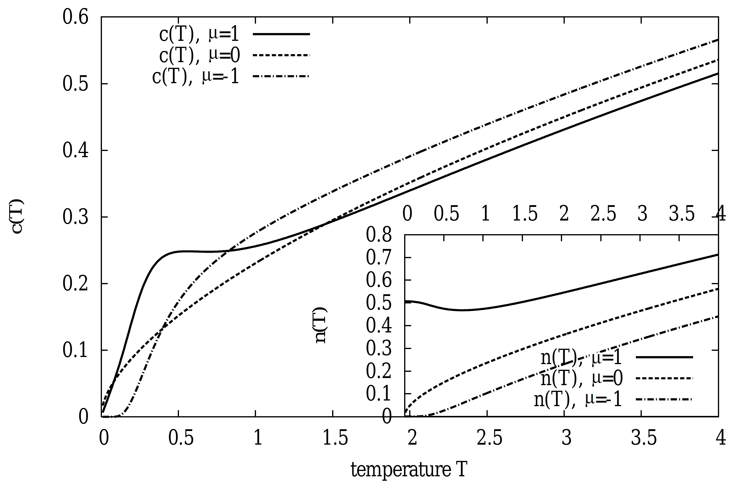
Figure 2: Thermodynamics: Specific heat as a function of temperature $T$ for three characteristic cases of the chemical potential $\mu=-1,0,+1$ and fixed interaction strength $c=2$. (Inset) Particle densities as functions of temperature. (All quantities in units of $c_{0},$ $T_{0},$ $\mu_{0}$ and $n_{0}$.)

Next, we like to present our results for the leading correlation length of the Green’s function. We calculate the distribution shown for the dense phase in Fig.7 by means of the above non-linear integral equation (12). First of all, we realize that due to the coupling of all roots and holes, a backflow effect sets in and the distribution shown in Fig.7 symmetrizes. And second, for lower temperatures all hole parameters including $k_{0}$ are below the real axis and all roots are above. For the numerical treatment of this distribution a straight integration contour is more suitable than the indented contour that allowed for a uniform treatment of the CFT properties. Choosing a straight contour for the case of $k_{0}$ below the real axis makes the contribution of $k_{0}$ to the driving term disappear, but imposes a severe change on the asymptotics of $\log\left(1+e^{-\overline{v}_{i}(k)/T}\right)$. This function converges to $0$ for $k\to-\infty$, but to $-2\pi$i for $k\to+\infty$. This modified asymptotics can be enforced numerically and yields the results shown in Fig.3.

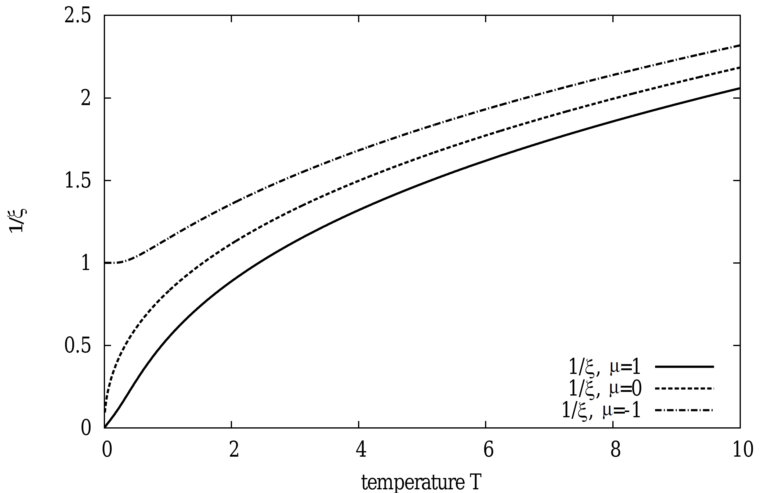
Figure 3: Green’s function: Reciprocal correlation length $1/\xi$ as a function of temperature $T$ for three characteristic cases of the chemical potential $\mu=-1,0,+1$ and fixed interaction strength $c=2$. (All quantities in units of $\xi_{0}^{-1},$ $T_{0}$ and $\mu_{0}$.)

Note that there is no oscillating $k_{F}$ factor for this correlation function. For $\mu<0$ the low temperature limit of $1/\xi(T)$ is finite, for the critical value $\mu=0$ we see a $1/\xi(T)\simeq T^{1/2}$ behaviour and for $\mu>0$ the CFT behaviour ${1/\xi(T)\simeq 2\pi\frac{T}{v_{F}}\frac{1}{4{\cal Z}^{2}}}$ sets in at low temperatures.

Finally, we present our results for the density-density correlator. The leading term is given by a “particle-hole excitation” at one Fermi point without $2k_{F}$ oscillations at low temperature, see (94). Interestingly, for this leading contribution there is a cross-over scenario at elevated temperatures from non-oscillating to oscillating behaviour. The detailed study of this phenomenon is beyond the scope of this publication. Therefore, we restrict ourselves to the study of the next-leading contribution with $2k_{F}$ oscillations at low temperatures with roots and holes as illustrated in Fig.6.

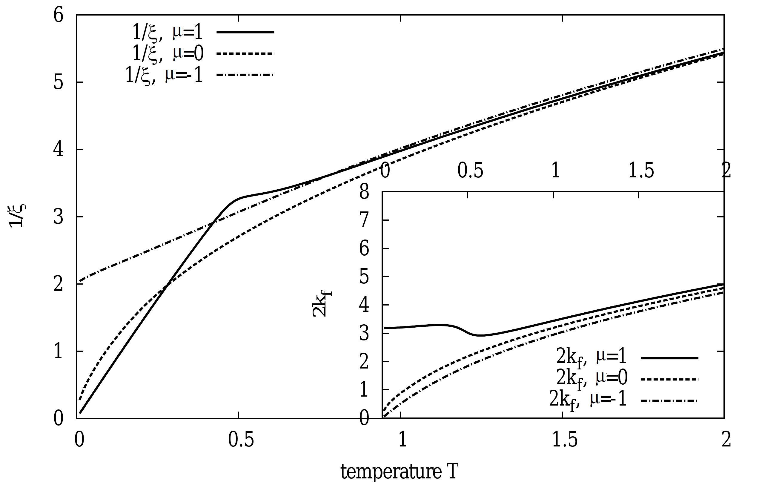
Figure 4: Density-density correlation function (2nd leading term): Reciprocal correlation length $1/\xi$ as a function of temperature $T$ for three characteristic cases of the chemical potential $\mu=-1,0,+1$ and fixed interaction strength $c=2$. (Inset) Wave number $2k_{F}$ of the oscillating factor. (All quantities in units of $\xi^{-1}_{0},$ $T_{0},$ $\mu_{0}$ and $k_{0}$.)

For $\mu<0$ the low temperature limit of $1/\xi(T)$ is finite, for the critical value $\mu=0$ we see a $1/\xi(T)\simeq T^{1/2}$ behaviour and for $\mu>0$ the CFT behaviour ${1/\xi(T)\simeq 2\pi\frac{T}{v_{F}}{{\cal Z}^{2}}}$ sets in at low temperatures. The oscillations $2k_{F}$ vanish at low $T$ for $\mu\leq 0$. In the dense phase ($\mu>0$) at low $T$ we expect the universal relation $2k_{F}(T)\simeq 2\pi n(T)$ which is nicely satisfied at very low $T$, see Fig.5, but shows a non-trivial temperature dependence at elevated $T$.

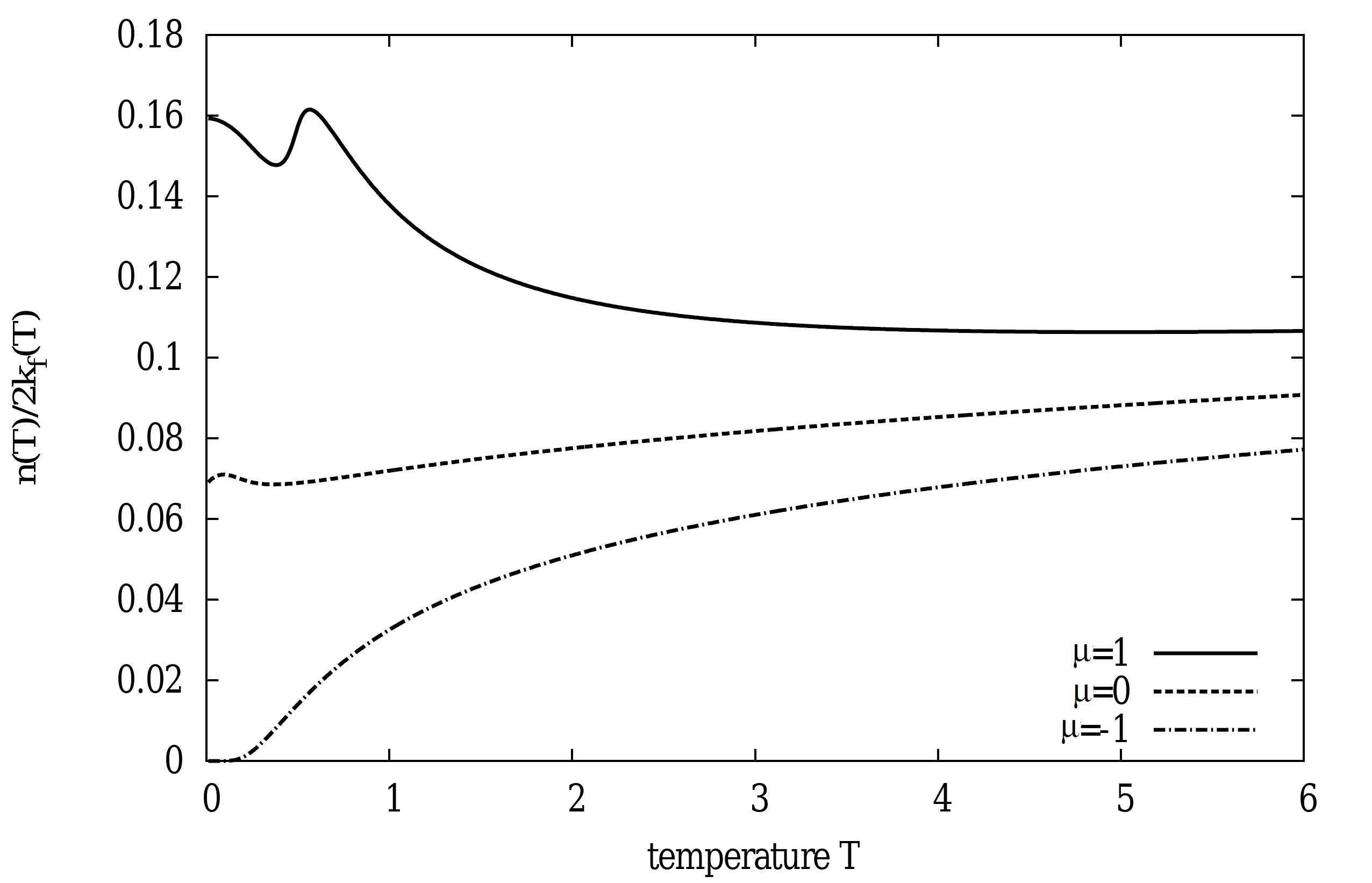
Figure 5: Density-density correlation function (2nd leading term): Particle number $n(T)$ divided by the wave number $2k_{F}(T)$ as a function of temperature $T$. Note for the case $\mu=+1$ the universal $T\to 0$ limit $1/2\pi$. (Temperature in units of $T_{0}$.)

We like to note that the dressed charge for $\mu=+1$ and $c=2$ takes the value ${\cal Z}=1.38$ consistent with the low-temperature behaviour of the correlators shown above.

VII Conclusions

Using the spectrum of the XXZ spin chain QTM and a specific continuum limit we have derived the asymptotic expansions of the temperature dependent density-density and field-field correlation functions in the interacting one-dimensional Bose gas. As a by-product we have also obtained similar expansions, valid at low-temperatures, for the longitudinal and transversal correlation functions in the XXZ spin chain. One could naturally expect that similar results can be derived in the case of the spinorial 1D Bose gas LGYE which can be obtained as the continuum limit of the $U_{q}(\hat{sl}(3))$ Perk-Schultz spin chain BVV ; dV . This subject will be deferred to a future publication.

VIII Acknowledgements

The authors would like to thank Frank Göhmann for numerous comments and discussions. Financial support from the VolkswagenStiftung and the PNII-RU-TE-2012-3-0196 grant of the Romanian National Authority for Scientific Research is gratefully acknowledged.

Note added in proof- Recently we become aware of DGK where some of the results for the XXZ spin chain were rederived and generalized.

Appendix A Derivation of the integral equations for the next-largest eigenvalues in the $N/2$ sector

A.1 Integral equation for the auxiliary function

For reasons of clarity we are going to consider first the simplest case in which only one Bethe root/hole is outside/inside the relevant strip in the complex plane. The generalization to the case of $r$ pairs is a natural extension of this particular example. A typical distribution of roots and holes for $\eta\in(0,\pi/2)$ and low-temperatures is presented in Fig. 6,

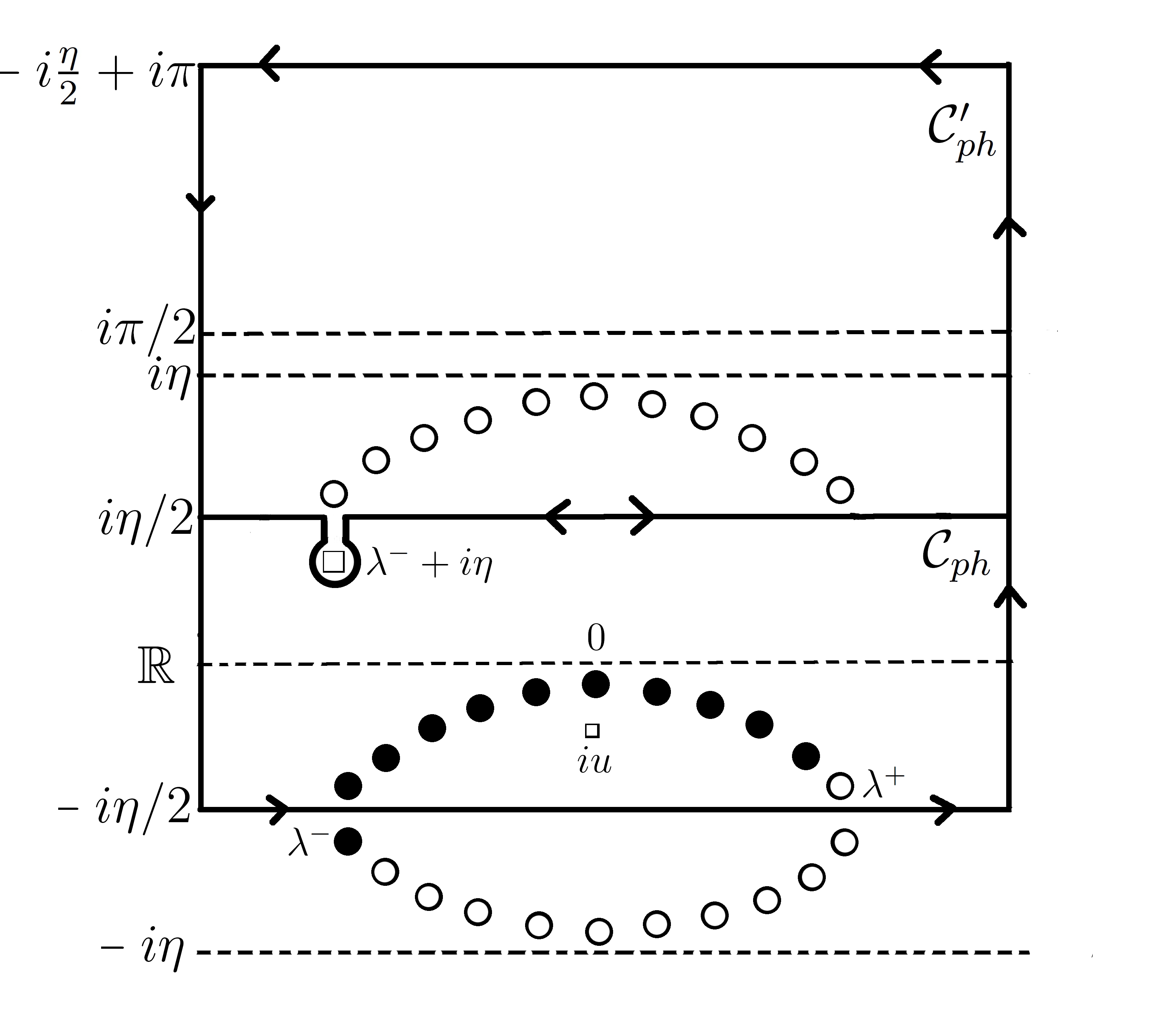
Figure 6: Typical distribution of Bethe roots ($\bullet$) and holes ($\circ$) in the strip $|\Im\lambda|<\eta\,,\eta\in[0,\pi/2)$ characterizing one of the next-largest eigenvalues of the QTM in the $N/2$ sector at low-temperature. All the other roots and holes can be obtained using the $i\pi$ periodicity. The indentation of the contour $\mathcal{C}_{ph}$ excludes $\lambda^{-}+i\eta$ and a hole located close to it. The lower edge of the contour $\mathcal{C}_{ph}^{\prime}$ is the same as the upper edge of $\mathcal{C}_{ph}$ but with different orientation. The contour $\mathcal{C}_{ph}$ surrounds all the Bethe roots except $\lambda^{-}$ the hole located at $\lambda^{+}$ and the pole of the auxiliary function $\mathfrak{a}_{ph}(\lambda)$ at $iu$.

where we have denoted by $\lambda^{-}$ and $\lambda^{+}$ the Bethe root, respectively, the hole outside (inside) the strip $|\Im\lambda|<\eta/2.$ It should be emphasized that this “particle-hole” distribution is valid only at low-temperatures, at higher temperatures the next-largest eigenvalues in the $N/2$ sector are characterized by the so-called 1-string type and 2-string type solutions KMSS . The eigenvalue and the auxiliary function $\mathfrak{a}_{ph}(\lambda)$ corresponding to the distribution presented in Fig. 6 are described by the same formulas as in (41) and (42). It is useful to present $q(\lambda)$ in the following form

$$q(\lambda)=\sinh(\lambda-\lambda^{-})\prod_{j=1}^{\frac{N}{2}-1}\sinh(\lambda-\lambda_{j})\,,$$

where $\{\lambda_{j}\}_{j=1}^{N/2-1}$ are the $N/2-1$ Bethe roots inside the strip $|\Im\lambda|<\eta/2.$ The equation $\mathfrak{a}_{ph}(\lambda)+1=0$ has $3N/2$ solutions, of which $N/2$ are the Bethe roots and $N$ are holes denoted by $\{\lambda^{(h)}_{j}\}_{j=1}^{N-1}$ and $\lambda^{+}.$

We introduce the rectangular contour $\mathcal{C}_{ph}$ (see Fig. 6) centered at the origin, extending to infinity with the edges parallel to the real axis through $\pm i(\eta-\epsilon)/2\,,$ $\epsilon\rightarrow 0$ which presents an indentation of the upper edge such that $\lambda^{-}+i\eta$ is not in the interior of the contour. Inside the contour $\mathcal{C}_{ph}$ the function $1+\mathfrak{a}_{ph}(\lambda)$ has $N/2$ zeros at the Bethe roots $\{\lambda_{j}\}_{j=1}^{N/2-1}$ and hole $\lambda^{+}$ and a pole of order $N/2$ at $iu$. Therefore, the function $\log(1+\mathfrak{a}_{ph}(\lambda))$ has no winding number around the contour (the presence of the indentation ensures that the function $\log(1+\mathfrak{a}_{ph}(\lambda))$ does not have an extra pole at $\lambda^{-}+i\eta$) allowing us to define ($\lambda$ is located outside the contour $\mathcal{C}_{ph}$)

$$f_{ph}(\lambda)\equiv\frac{1}{2\pi i}\int_{\mathcal{C}_{ph}}\frac{d}{d\lambda}\left(\log\sinh(\lambda-\mu)\right)\log(1+\mathfrak{a}_{ph}(\mu))d\mu=\frac{1}{2\pi i}\int_{\mathcal{C}_{ph}}\log\sinh(\lambda-\mu)\frac{\mathfrak{a}_{ph}^{\prime}(\mu)}{1+\mathfrak{a}_{ph}(\mu)}d\mu\,,$$ (97)

which can be evaluated using Theorem 1 with the result

$$f_{ph}(\lambda)=\sum_{j=1}^{N/2-1}\log\sinh(\lambda-\lambda_{j})+\log\sinh(\lambda-\lambda^{+})-\frac{N}{2}\log\sinh(\lambda-iu)\,.$$ (98)

Eq. (98) which can be rewritten as $\log q(\lambda)=f_{ph}(\lambda)+\log\sinh(\lambda-\lambda^{-})-\log\sinh(\lambda-\lambda^{+})+\log\phi_{-}(\lambda)+N/2\log\sin\eta$ providing an integral representation for $\log q(\lambda).$ Taking the logarithm of Eq. (42) and using this integral representation we find

$$\log\mathfrak{a}_{ph}(\lambda)=-\beta h+\log\left(\frac{\phi_{+}(\lambda)}{\phi_{-}(\lambda)}\frac{\phi_{-}(\lambda+i\eta)}{\phi_{+}(\lambda+i\eta)}\right)+\log\left(\frac{\sinh(\lambda-\lambda^{-}+i\eta)}{\sinh(\lambda-\lambda^{-}-i\eta)}\right)-\log\left(\frac{\sinh(\lambda-\lambda^{+}+i\eta)}{\sinh(\lambda-\lambda^{+}-i\eta)}\right)+f_{ph}(\lambda+i\eta)-f_{ph}(\lambda-i\eta)\,.$$

Performing the Trotter limit, $N\rightarrow\infty$, with the help of Eq. (45) we obtain the NLIE for the auxiliary function

$$\log\mathfrak{a}_{ph}(\lambda) =-\beta e_{0}(\lambda+i\eta/2)+i\theta(\lambda-\lambda^{+})-i\theta(\lambda-\lambda^{-})-\frac{1}{2\pi}\int_{\mathcal{C}_{ph}}K(\lambda-\mu)\log(1+\mathfrak{a}_{ph}(\mu))d\mu\,.$$ (99)

Eq. (99) was obtained assuming $\eta\in(0,\pi/2).$ It remains valid also for $\eta\in(\pi/2,\pi)$ if the contour $\mathcal{C}_{ph}$ is replaced by a similar rectangular contour with the upper (lower) edges parallel to the real axis through $\pm i(\pi-\eta-\epsilon)/2\,,\epsilon\rightarrow 0$ but, in this case, without the indentation.

A.2 Integral expression for the next-largest eigenvalue in the $N/2$ sector

The integral expression for the next-largest eigenvalue in the $N/2$ sector is obtained in a similar fashion as in the largest eigenvalue case. The starting point is, again, the representation (49) of the eigenvalue in terms of the holes where it is useful to denote $q^{(h)}(\lambda)$ as

$$q^{(h)}(\lambda)=\sinh(\lambda-\lambda^{+})\prod_{j=1}^{N-1}\sinh(\lambda-\lambda_{j}^{(h)})\,.$$

In order to obtain an integral expression for $q^{(h)}(\lambda)$ we introduce a rectangular contour $\mathcal{C}_{ph}^{\prime}$ (see Fig. 6) extending to infinity with the edges parallel to the real axis through $i(\eta-\epsilon)/2$ and $-i(\eta-\epsilon)/2+i\pi.$ The edge at $i(\eta-\epsilon)/2$ presents an indentation such that $\lambda_{-}+i\eta$ is contained in the interior of $\mathcal{C}_{ph}^{\prime}$ and is identical with the upper edge of the contour $\mathcal{C}_{ph}$ but with opposite orientation. Then the following identity

$$\int_{\mathcal{C}_{ph}+\mathcal{C}_{ph}^{\prime}}d(\lambda-\mu)\frac{\mathfrak{a}_{ph}^{\prime}(\mu)}{1+\mathfrak{a}_{ph}(\mu)}d\mu=0\,,$$ (100)

can be proved in exactly the same way as its largest eigenvalue counterpart (50). For $\lambda$ close to the real axis using (100) and Theorem 1 we obtain

$$\frac{1}{2\pi i}\int_{\mathcal{C}_{ph}}d(\lambda-\mu)\frac{\mathfrak{a}_{ph}^{\prime}(\mu)}{1+\mathfrak{a}_{ph}(\mu)}d\mu =-\left(\sum_{j=1}^{N-1}d(\lambda-\lambda_{j}^{(h)})+d(\lambda-\lambda^{-})-d(\lambda-\lambda^{-}-i\eta)\right.$$

$$\ \ \ \ \ \ \ \ \ \ \ \ \ \ \ \ \ \ \ \ \ \ \ \ \ \ \left.-\sum_{j=1}^{N/2-1}d(\lambda-\lambda_{j}-i\eta)-\frac{N}{2}d(\lambda+iu+i\eta)\right)\,.$$ (101)

In deriving Eq. (A.2), we have used the fact that, inside the contour $\mathcal{C}_{ph}^{\prime},$ the function $1+\mathfrak{a}_{ph}(\lambda)$ has: $N$ zeros at $\lambda^{-}+i\pi,$ $\{\lambda_{j}^{(h)}\}_{j=1}^{N-1}$ or $\{\lambda_{j}^{(h)}\}_{j=1}^{N-1}+i\pi\,,$ $N/2-1$ simple poles at $\{\lambda_{j}\}_{j=1}^{N/2-1}+i\eta$, a simple pole at $\lambda^{-}+i\eta$ and a pole of order $N/2$ at $-iu-i\eta+i\pi$. Using again Theorem 1 and the fact that inside the contour $\mathcal{C}_{ph}$ the function $1+\mathfrak{a}_{ph}(\lambda)$ has: $N/2$ zeros at the Bethe roots $\{\lambda_{j}\}_{j=1}^{N/2-1}$ and hole $\lambda^{+}$, and a pole of order $N/2$ at $iu$ we find

$$\frac{1}{2\pi i}\int_{\mathcal{C}_{ph}}d(\lambda-\mu-i\eta)\frac{\mathfrak{a}_{ph}^{\prime}(\mu)}{1+\mathfrak{a}_{ph}(\mu)}d\mu=\sum_{j=1}^{N/2-1}d(\lambda-\lambda_{j}-i\eta)+d(\lambda-\lambda^{+}-i\eta)-\frac{N}{2}d(\lambda-iu-i\eta)\,.$$ (102)

Taking the difference of Eqs. (A.2) and (102), integrating by parts, and then integrating w.r.t. $\lambda$ we obtain the following representation

$$\log q^{(h)}(\lambda) =\log\left(\frac{\sinh(\lambda-\lambda^{+})}{\sinh(\lambda-\lambda^{+}-i\eta)}\right)-\log\left(\frac{\sinh(\lambda-\lambda^{-})}{\sinh(\lambda-\lambda^{-}-i\eta)}\right)+\log\left(\phi_{+}(\lambda+i\eta)\phi_{-}(\lambda-i\eta)\right)$$

$$\ \ \ \ \ \ \ \ \ \ \ \ \ \ \ \ -\frac{1}{2\pi i}\int_{\mathcal{C}_{ph}}\left[d(\lambda-\mu)-d(\lambda-\mu-i\eta)\right]\log(1+\mathfrak{a}_{ph}(\mu))\,d\mu+c\,,$$ (103)

with $c$ a constant of integration. Finally, the integral expression for the next-largest eigenvalue of the QTM in the $N/2$ sector is obtained by replacing (A.2) in (49) with the result

$$\log\Lambda_{ph}(0)=\frac{\beta h}{2}+\log\left(\frac{\sinh\lambda^{+}}{\sinh(\lambda^{+}+i\eta)}\right)-\log\left(\frac{\sinh\lambda^{-}}{\sinh(\lambda^{-}+i\eta)}\right)+\frac{1}{2\pi}\int_{\mathcal{C}_{ph}}p_{0}^{\prime}(\mu+i\eta/2)\log(1+\mathfrak{a}_{ph}(\mu))d\mu\,.$$ (104)

The constant of integration, $\beta h/2,$ was calculated using the behavior of the involved functions at infinity, like in the case of the largest eigenvalue. Eq. (104) is also valid in the domain $\eta\in(\pi/2,\pi)$ if the contour $\mathcal{C}_{ph}$ is replaced by a rectangular contour, extending to infinity, with the edges parallel to the real axis through $\pm i(\pi-\eta-\epsilon)/2\,,$ $\epsilon\rightarrow 0$.

A.3 Final form of the integral equations

We consider $\eta\in(0,\pi/2)$. In the low-temperature limit we are going to neglect the contribution from the upper edge of the contour as we did in Sec. IV.1.3. If in Eq. (99) we restrict the free parameter $\lambda$ and the variable of integration to the lower part of the contour which is the line parallel to the real axis at $-i\eta/2$ we find

$$\log\mathfrak{a}_{ph}(\lambda-i\eta/2) =-\beta e_{0}(\lambda)+i\theta(\lambda-\lambda^{+})-i\theta(\lambda-\lambda^{-})-\frac{1}{2\pi}\int_{\mathbb{R}}K(\lambda-\mu)\log(1+\mathfrak{a}_{ph}(\mu-i\eta/2))d\mu\,,$$ (105)

where by $\lambda^{\pm}$ we understand $\lambda^{\pm}\rightarrow\lambda^{\pm}+i\eta/2\,,$ which now belong to the upper (lower) half-plane. The expression (104) for the next-largest eigenvalue becomes

$$\log\Lambda_{ph}(0) =\frac{\beta h}{2}+ip_{0}(\lambda^{+})-ip_{0}(\lambda^{-})+\frac{1}{2\pi}\int_{\mathbb{R}}p_{0}^{\prime}(\mu)\log(1+\mathfrak{a}_{ph}(\mu-i\eta/2))d\mu\,.$$ (106)

Introducing the function $u(\lambda)$ satisfying $e^{-u(\lambda)/T}=\mathfrak{a}_{ph}(\lambda-i\eta/2),$ the NLIE for the auxiliary function and the integral expression for the next-largest eigenvalues in the $N/2$ sector at low-temperatures can be written as

$$u(\lambda)=e_{0}(\lambda)-iT\theta(\lambda-\lambda^{+})+iT\theta(\lambda-\lambda^{-})+\frac{T}{2\pi}\int_{\mathbb{R}}K(\lambda-\mu)\log\left(1+e^{-u(\mu)/T}\right)d\mu\,,$$ (107)

$$\log\Lambda_{ph}(0)=\frac{h}{2T}+ip_{0}(\lambda^{+})-ip_{0}(\lambda^{-})+\frac{1}{2\pi}\int_{\mathbb{R}}p_{0}^{\prime}(\mu)\log\left(1+e^{-u(\mu)/T}\right)d\mu\,,$$ (108)

where the parameters $\lambda^{\pm}$ satisfy the constraint $1+e^{-u(\lambda^{\pm})/T}=0,$ and are located in the upper (lower) half-plane. While we derived these equations assuming that $\eta\in(0,\pi/2)$ we are going to assume that they are valid also for $\eta\in(\pi/2,\pi)$. The CFT analysis in Sec.V shows that this assumption is justified. The obvious generalization of Eqs. (107) and (108) in the case of $r$ pairs of Bethe roots and holes is given by Eqs. (60) and (59).

Appendix B Derivation of the integral equations for the next-largest eigenvalues in the $N/2-1$ sector

B.1 Integral equation for the auxiliary function

As we have mentioned in Sec. IV.3 it is sufficient to consider the case with $N/2-1$ Bethe roots and, possibly, one hole in the relevant strip of the complex plane. First, we will consider the case with one hole inside the strip. A typical distribution of the Bethe roots and hole, at low-temperatures and $\eta\in(0,\pi/2)$, is presented in Fig. 7, where we have denoted by $\lambda_{0}$ the hole inside the strip $|\Im\lambda|<\eta/2.$ The eigenvalue and auxiliary function $\mathfrak{a}_{s}(\lambda)$ corresponding to the distribution presented in Fig. 7

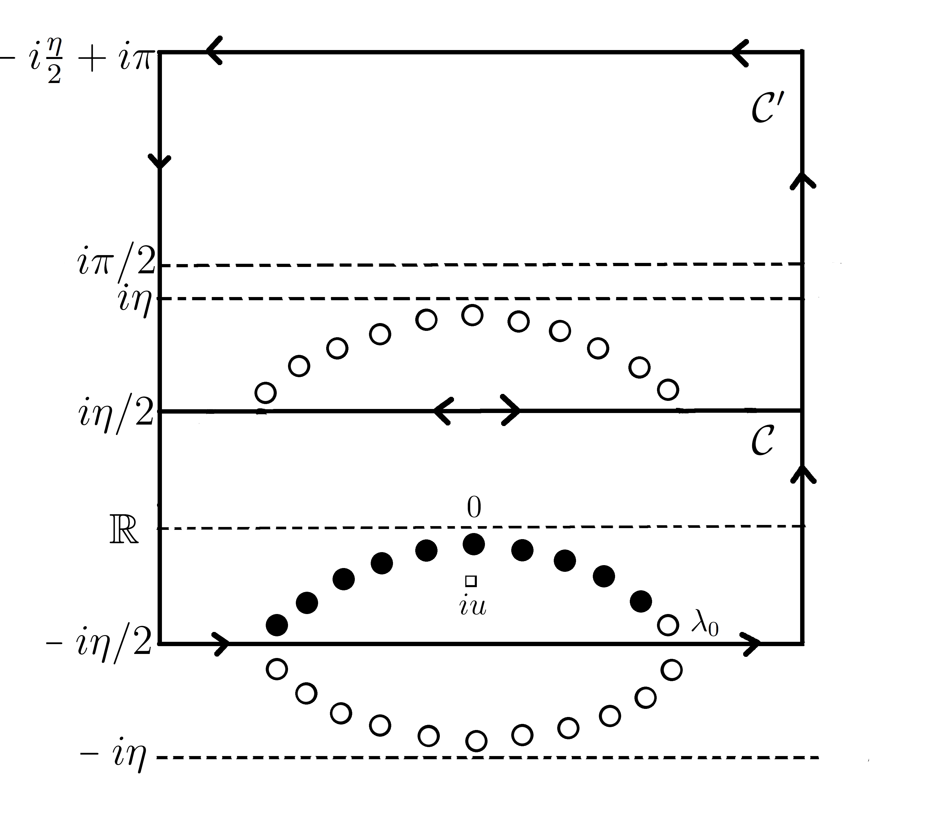
Figure 7: Typical distribution of Bethe roots ($\bullet$) and holes ($\circ$) in the strip $|\Im\lambda|<\eta\,,\eta\in[0,\pi/2)$ characterizing the next-largest eigenvalues of the QTM in the $N/2-1$ sector without “particle-hole” type terms. All the other roots and holes can be obtained using the $i\pi$ periodicity. The contour $\mathcal{C}$ surrounds all the Bethe roots, the hole located at $\lambda_{0}$ and the pole of the auxiliary function $\mathfrak{a}_{s}(\lambda)$ at $iu$.

are described by formulas similar to (41) and (42), but in this case $q(\lambda)$ is defined as

$$q(\lambda)=\prod_{j=1}^{\frac{N}{2}-1}\sinh(\lambda-\lambda_{j})\,,$$

where $\{\lambda_{j}\}_{j=1}^{N/2-1}$ are the $N/2-1$ Bethe roots. The equation $\mathfrak{a}_{s}(\lambda)+1=0$ has $3N/2-1$ solutions, of which, $N/2-1$ are Bethe roots and $N$ are holes denoted by $\{\lambda^{(h)}\}_{j=1}^{N-1}$ and $\lambda_{0}$.

Consider the contour $\mathcal{C}$ introduced in Sec. IV.1.1. Inside the contour, the function $1+\mathfrak{a}_{s}(\lambda)$ has $N/2$ zeros at the Bethe roots $\{\lambda_{j}\}_{j=1}^{N/2-1}$ and hole $\lambda_{0}$, and a pole of order $N/2$ at $iu$. Therefore, we can define ($\lambda$ is located outside the contour $\mathcal{C}$)

$$f_{s}(\lambda)\equiv\frac{1}{2\pi i}\int_{\mathcal{C}}\frac{d}{d\lambda}\left(\log\sinh(\lambda-\mu)\right)\log(1+\mathfrak{a}_{s}(\mu))d\mu=\frac{1}{2\pi i}\int_{\mathcal{C}}\log\sinh(\lambda-\mu)\frac{\mathfrak{a}_{s}^{\prime}(\mu)}{1+\mathfrak{a}_{s}(\mu)}d\mu\,,$$ (109)

which can be evaluated using Theorem 1 with the result

$$f_{s}(\lambda)=\sum_{j=1}^{N/2-1}\log\sinh(\lambda-\lambda_{j})+\log\sinh(\lambda-\lambda_{0})-\frac{N}{2}\log\sinh(\lambda-iu)\,.$$ (110)

Taking the logarithm in Eq. (42), and using (110), which can be rewritten as $\log q(\lambda)=f_{s}(\lambda)-\log\sinh(\lambda-\lambda_{0})+\log\phi_{-}(\lambda)+N/2\log\sin\eta$ we find

$$\log\mathfrak{a}_{s}(\lambda)=-\beta h+\log\left(\frac{\phi_{+}(\lambda)}{\phi_{-}(\lambda)}\frac{\phi_{-}(\lambda+i\eta)}{\phi_{+}(\lambda+i\eta)}\right)+\log\left(\frac{\sinh(\lambda-\lambda_{0}-i\eta)}{\sinh(\lambda-\lambda_{0}+i\eta)}\right)+f_{s}(\lambda+i\eta)-f_{s}(\lambda-i\eta)\,.$$

Making use of Eq. (45), we can take the Trotter limit, $N\rightarrow\infty,$ obtaining the NLIE for the auxiliary function

$$\log\mathfrak{a}_{s}(\lambda) =-\beta e_{0}(\lambda+i\eta/2)\mp i\pi+i\theta(\lambda-\lambda_{0})-\frac{1}{2\pi}\int_{\mathcal{C}}K(\lambda-\mu)\log(1+\mathfrak{a}_{s}(\mu))d\mu\,.$$ (111)

In Eq. (111), the minus (plus) sign in front of the $i\pi$ factor is considered when $\Re\lambda_{0}$ is positive (negative). The same NLIE is valid also for $\eta\in(\pi/2,\pi)$ if the contour $\mathcal{C}$ is replaced by a similar rectangular contour with the upper (lower) edges parallel to the real axis through $\pm i(\pi-\eta-\epsilon)/2\,,\epsilon\rightarrow 0.$

B.2 Integral expression for the next-largest eigenvalue in the $N/2-1$ sector

The starting point of our derivation will be again the representation (49), which is also valid for the eigenvalues in the $N/2-1$ sector. We need an integral representation for $q^{(h)}(\lambda)=\sinh(\lambda-\lambda_{0})\prod_{j=1}^{N-1}\sinh(\lambda-\lambda_{j}^{(h)})\,$. If we consider the contour $\mathcal{C}^{\prime}$ introduced in IV.1.2, then the following identity holds

$$\int_{\mathcal{C}+\mathcal{C}^{\prime}}d(\lambda-\mu)\frac{\mathfrak{a}_{s}^{\prime}(\mu)}{1+\mathfrak{a}_{s}(\mu)}d\mu=0\,.$$ (112)

For $\lambda$ close to the real axis, using (112), Theorem 1 and the fact that inside the contour $\mathcal{C}_{ph}^{\prime}$ the function $1+\mathfrak{a}_{s}(\lambda)$ has: $N-1$ zeros at $\{\lambda_{j}^{(h)}\}_{j=1}^{N-1}$ or $\{\lambda_{j}^{(h)}\}_{j=1}^{N-1}+i\pi\,,$ $N/2-1$ simple poles at $\{\lambda_{j}\}_{j=1}^{N/2-1}+i\eta$ and a pole of order $N/2$ at $-iu-i\eta+i\pi$, we find

$$\frac{1}{2\pi i}\int_{\mathcal{C}}d(\lambda-\mu)\frac{\mathfrak{a}_{s}^{\prime}(\mu)}{1+\mathfrak{a}_{s}(\mu)}d\mu=-\left(\sum_{j=1}^{N-1}d(\lambda-\lambda_{j}^{(h)})-\sum_{j=1}^{N/2-1}d(\lambda-\lambda_{j}-i\eta)-\frac{N}{2}d(\lambda+iu+i\eta)\right)\,.$$ (113)

Inside the contour $\mathcal{C}$ the function $1+\mathfrak{a}_{s}(\lambda)$ has $N/2$ zeros at the Bethe roots $\{\lambda_{j}\}_{j=1}^{N/2-1}$ and hole $\lambda_{0}$ and a pole of order $N/2$ at $iu$. Using again Theorem 1 we have

$$\frac{1}{2\pi i}\int_{\mathcal{C}}d(\lambda-\mu-i\eta)\frac{\mathfrak{a}_{s}^{\prime}(\mu)}{1+\mathfrak{a}_{s}(\mu)}d\mu=\sum_{j=1}^{N/2-1}d(\lambda-\lambda_{j}-i\eta)+d(\lambda-\lambda_{0}-i\eta)-\frac{N}{2}d(\lambda-iu-i\eta)\,.$$ (114)

Taking the difference of Eqs. (113) and (114), integrating by parts, and then integrating w.r.t. $\lambda$ we obtain the following representation

$$\log q^{(h)}(\lambda) =\log\left(\frac{\sinh(\lambda-\lambda_{0})}{\sinh(\lambda-\lambda_{0}-i\eta)}\right)+\log\left(\phi_{+}(\lambda+i\eta)\phi_{-}(\lambda-i\eta)\right)$$

$$\ \ \ \ \ \ \ \ \ \ \ \ \ \ \ \ \ \ \ \ \ \ \ \ \ \ \ \ \ -\frac{1}{2\pi i}\int_{\mathcal{C}}\left[d(\lambda-\mu)-d(\lambda-\mu-i\eta)\right]\log(1+\mathfrak{a}_{s}(\mu))d\mu+c\,,$$ (115)

with $c$ a constant of integration. The integral expression for the next-largest eigenvalue of the QTM in the sector $N/2-1$ is obtained by replacing (B.2) in (49) with the result

$$\log\Lambda_{s}(0)=\frac{\beta h}{2}+\log\left(\frac{\sinh\lambda_{0}}{\sinh(\lambda_{0}+i\eta)}\right)+\frac{1}{2\pi}\int_{\mathcal{C}}p_{0}^{\prime}(\mu+i\eta/2)\log(1+\mathfrak{a}_{s}(\mu))d\mu\,.$$ (116)

Eq. (116) is also valid in the domain $\eta\in(\pi/2,\pi)$ if the contour $\mathcal{C}$ is replaced by a rectangular contour, extending to infinity, with the edges parallel to the real axis through $\pm i(\pi-\eta-\epsilon)/2\,,$ $\epsilon\rightarrow 0$.

B.3 Final form of the integral equations

We consider $\eta\in(0,\pi/2)$. Performing the same operations as in Appendix A.3, Eq. (111) is transformed into

$$\log\mathfrak{a}_{s}(\lambda-i\eta/2) =-\beta e_{0}(\lambda)\mp i\pi+i\theta(\lambda-\lambda_{0})-\frac{1}{2\pi}\int_{\mathbb{R}}K(\lambda-\mu)\log(1+\mathfrak{a}_{s}(\mu-i\eta/2))d\mu\,,$$ (117)

where $\lambda_{0}\rightarrow\lambda_{0}+i\eta/2\,$ is in the upper half-plane. The expression (116) for the next-largest eigenvalue becomes

$$\log\Lambda_{s}(0) =\frac{\beta h}{2}-i\pi+ip_{0}(\lambda_{0})+\frac{1}{2\pi}\int_{\mathbb{R}}p_{0}^{\prime}(\mu)\log(1+\mathfrak{a}_{s}(\mu-i\eta/2))d\mu\,.$$ (118)

Introducing the function $v(\lambda)$ satisfying $e^{-v(\lambda)/T}=\mathfrak{a}_{s}(\lambda-i\eta/2)$ the NLIE for the auxiliary function and the integral expression for the next-largest eigenvalues in the $N/2-1$ sector at low-temperatures can be written as

$$v(\lambda)=e_{0}(\lambda)\pm i\pi T-iT\theta(\lambda-\lambda_{0})+\frac{T}{2\pi}\int_{\mathbb{R}}K(\lambda-\mu)\log\left(1+e^{-v(\mu)/T}\right)d\mu\,,$$ (119)

$$\log\Lambda_{s}(0)=\frac{h}{2T}-i\pi+ip_{0}(\lambda_{0})+\frac{1}{2\pi}\int_{\mathbb{R}}p_{0}^{\prime}(\mu)\log\left(1+e^{-v(\mu)/T}\right)d\mu\,,$$ (120)

where $\lambda_{0}$ satisfies the constraint $1+e^{-v(\lambda_{0})/T}=0$. We should mention that we can discard the $i\pi$ term on the r.h.s. of (120) (this has the effect of neglecting an $(-1)^{m}$ factor in the asymptotic expansion which is irrelevant in the continuum limit) On the r.h.s. of Eq. (119) we will consider the plus (minus) sign in front of the $i\pi T$ term when $\lambda_{0}$ is in the first (second) quadrant of the complex plane. Again we are going to assume that similar formulas are valid for $\eta\in(\pi/2,\pi)$. The generalization of (119) and (120) to the case when $r$ “particle-hole” pairs are present is given by Eqs. (61) and (62).

We still need to derive equations for the case when inside the strip $|\Im\lambda|<\eta/2$ there is no hole present. Consider $\lambda_{0}$ the hole closest to the line parallel to the real axis with imaginary part $-i\eta/2$. If we modify $\mathcal{C}$ adding an indentation such that $\lambda_{0}$ is inside the contour and similarly modifying the upper edge of $\mathcal{C}^{\prime}$ such that $\lambda_{0}+i\pi$ is outside of $\mathcal{C}^{\prime}$ then all the considerations of the previous sections still hold. However, when we take the low-temperature limit of the equations in Eqs. (117) and (118) the integration contour will be transformed in the real axis with an indentation such that $\lambda_{0}\rightarrow\lambda_{0}+i\eta/2$ (which now belongs to the lower half-plane) is above the contour. The generalization of this result to the case when $r$ “particle-hole” pairs are present is presented in Sect. IV.3.

Appendix C Proof of some identities

Here we prove some identities used in Sec. V. We start with

$$\int_{-q}^{q}p_{0}^{\prime}(\lambda)R(\lambda,\pm q)\,d\lambda=p_{0}^{\prime}(q)-2\pi\rho(q)\,.$$ (121)

Using a formal solution of Eq. (24) on the l.h.s. of (121) we have

$$\int_{-q}^{q}p_{0}^{\prime}(\lambda)R(\lambda,\pm q)\,d\lambda =\int_{-q}^{q}\int_{-q}^{q}\left(1+\frac{1}{2\pi}K\right)^{-1}(\lambda,\mu)\,\frac{1}{2\pi}K(\mu\mp q)p_{0}^{\prime}(\lambda)\,d\mu\,d\lambda\,,$$

$$=\int_{-q}^{q}K(q\mp\mu)\rho(\mu)d\mu\,,$$

where in the second line we have used the symmetry of the kernel $K(\lambda-\mu)=K(\mu-\lambda)$ and the integral equation for the density (21). The identity (121) follows from

$$\rho(\pm q)+\frac{1}{2\pi}\int_{-q}^{q}K(q\mp\mu)\rho(\mu)\,d\mu=\frac{1}{2\pi}p_{0}^{\prime}(\pm q)\,,$$ (122)

and the fact that $\rho(\lambda)$ and $p_{0}^{\prime}(\lambda)$ are even functions. Using a similar method we can prove that

$$\int_{-q}^{q}\varepsilon_{0}(\lambda)p_{0}^{\prime}(\lambda)\,d\lambda=2\pi\int_{-q}^{q}e_{0}(\lambda)\rho(\lambda)\,d\lambda.$$ (123)

Making use of the equation for the dressed energy (22) we can rewrite the l.h.s. of (123) as

$$\int_{-q}^{q}\varepsilon_{0}(\lambda)p_{0}^{\prime}(\lambda)\,d\lambda =\int_{-q}^{q}\int_{-q}^{q}\left(1+\frac{1}{2\pi}K\right)^{-1}(\lambda,\mu)\,e_{0}(\mu)\,p_{0}^{\prime}(\lambda)\,d\mu\,d\lambda\,,$$

$$=2\pi\int_{-q}^{q}e_{0}(\mu)\rho(\mu)d\mu\,,$$

where we have used again the symmetry of the kernel and Eq. (21).

Appendix D Derivation of the asymptotic expansion for the generating functional of density correlators

In this Appendix we will show how we can derive using our method the results obtained in KMS1 ; KMS2 . The first step in the computation of the asymptotic expansion for the generating functional of density correlators in the Bose gas is the derivation of NLIEs for the eigenvalues of the twisted QTM $\textsf{t}^{QTM}_{\varphi}=A^{QTM}(0)+e^{\varphi}D^{QTM}(0)$ in the $N/2$ sector. The eigenvalues of the twisted QTM in the $N/2$ sector are GKS1 :

$$\Lambda_{i}^{(\varphi)}(\lambda)=\frac{\phi_{-}(\lambda)}{\phi_{-}(\lambda-i\eta)}\frac{q(\lambda-i\eta)}{q(\lambda)}e^{\frac{\beta h}{2}}+\frac{\phi_{+}(\lambda)}{\phi_{+}(\lambda+i\eta)}\frac{q(\lambda+i\eta)}{q(\lambda)}e^{-\frac{\beta h}{2}+\varphi}\,,$$ (124)

with $q(\lambda)=\prod_{j=1}^{N/2}\sinh(\lambda-\lambda_{j})$ and $\{\lambda_{j}\}_{j=1}^{N/2}$ satisfying the BAEs

$$\left(\frac{b(u^{\prime},\lambda_{j})}{b(\lambda_{j},-u^{\prime})}\right)^{N/2}=e^{-\beta h+\varphi}\prod_{j\neq k}^{N/2}\frac{\sinh(\lambda_{j}-\lambda_{k}+i\eta)}{\sinh(\lambda_{j}-\lambda_{k}-i\eta)}\,,\ \ \ \ j=1,\cdots,N/2\,.$$ (125)

The derivation of the NLIEs and integral expressions for the $N/2$ sector eigenvalues of the twisted QTM (this includes also the largest eigenvalue) is almost identical with the one presented in Section IV.1 and Appendix A (we use a similar distribution of Bethe roots and holes as in Fig. 1 and Fig. 6). We obtain similar equations as Eqs. (58a) and (58b) (for the largest eigenvalue) and Eqs. (59) and (60) (for the next-largest eigenvalues in the $N/2$ sector) with the only difference being the replacement of the $h/(2T)$ with $h/(2T)+\varphi T$ in the r.h.s. of Eqs. (58b) and (60). The reader should note that $\varphi$ does not appear in the integral expressions for the eigenvalues.

Performing the continuum limit in (40) we find

$$\langle e^{\varphi\int_{0}^{x}j(x^{\prime})\,dx^{\prime}}\rangle_{T} =\sum_{i}\tilde{C}_{i}e^{-\frac{x}{\xi^{(\varphi)}[\overline{u}_{i}^{\varphi}]}}\,,\ \ \ \ \ x\rightarrow\infty\,,$$ (126)

with the correlation lengths defined by

$$\frac{1}{\xi^{(\varphi)}[\overline{u}_{i}^{\varphi}]}=-\frac{1}{2\pi}\int_{\mathbb{R}}\log\left(\frac{1+e^{-\overline{u}_{i}^{\varphi}(k)/T}}{1+\,e^{-\overline{\varepsilon}(k)/T}}\right)\,dk-i\sum_{j=1}^{r}k^{+}_{j}+i\sum_{j=1}^{r}k^{-}_{j}\,,$$ (127)

and the auxiliary functions $\overline{u}_{i}^{\varphi}(k)$ satisfying the NLIEs:

$$\overline{u}_{i}^{\varphi}(k)=k^{2}-\mu-\varphi T+iT\sum_{j=1}^{r}\overline{\theta}(k-k^{+}_{j})-iT\sum_{j=1}^{r}\overline{\theta}(k-k^{-}_{j})-\frac{T}{2\pi}\int_{\mathbb{R}}\overline{K}(k-k^{\prime})\log\left(1+e^{-\overline{u}_{i}^{\varphi}(k^{\prime})/T}\right)dk^{\prime}\,.$$ (128)

The $2r$ parameters, $\{k^{+}_{j}\}_{j=1}^{r}\,(\{k^{-}_{j}\}_{j=1}^{r})$ appearing in Eq. (128) belong to the upper (lower) half of the complex plane and satisfy the constraint $1+e^{\overline{u}_{i}^{\varphi}(k^{\pm}_{j})/T}=0.$ $r$ can take the values $0,1,2,\cdots$ with the $r=0$ term (this means that the sums in Eq. (127), (128) are zero) being the dominant contribution in the expansion. Eq. (126) was first derived in KMS1 .

Appendix E Low-temperature limit of the asymptotic expansions

The low-temperature analysis of the asymptotic expansions (10) and (13) is very similar with the one performed in Sec. V.2 and V.3. The only difference is the fact that in the Bose gas case the principal integral operator is $I-\frac{1}{2\pi}\overline{K}$ and $p_{0}(k)=k$ which means that $p_{0}^{\prime}(k)=1$. Therefore, the calculations are almost identical with the ones for the XXZ spin chain except for some sign changes. The integral equations for the zero temperature dressed energy $\overline{\varepsilon}_{0}(k)$ and the dressed charge $\overline{Z}(k)$ are given by

$$\overline{\varepsilon}_{0}(k)-\frac{1}{2\pi}\int_{-\overline{q}}^{\overline{q}}\overline{K}(k-k^{\prime})\overline{\varepsilon}_{0}(k^{\prime})\,dk^{\prime}=k^{2}-\mu\equiv\overline{e}_{0}(k)\,,$$ (129)

and

$$\overline{Z}(k)-\frac{1}{2\pi}\int_{-\overline{q}}^{\overline{q}}\overline{K}(k-k^{\prime})\overline{Z}(k^{\prime})\,dk^{\prime}=1\,,\ \ \ \ \ \ \overline{Z}(\pm\overline{q})=\overline{\mathcal{Z}}\,.$$ (130)

The resolvent of the integral operator $I-\frac{1}{2\pi}\overline{K}$ and the dressed phase equations are obtained from the XXZ spin chain equivalents, (24) and (25), by changing the sign in front of the integral and replacing $K(\lambda,\mu)\,,\theta(\lambda)$ and $\pm q$ with $\overline{K}(k,k^{\prime})\,,\overline{\theta}(k)$ and $\pm\overline{q}.$ The identities (26)and (121) transform into (note the sign changes)

$$\overline{Z}(k)=1+\overline{F}(k|-\overline{q})-\overline{F}(k|\overline{q})\,,\ \ \ \ \frac{1}{\overline{\mathcal{Z}}}=1-\overline{F}(\overline{q}|\overline{q})-\overline{F}(\overline{q}|-\overline{q})\,,$$ (131)

$$\int_{-\overline{q}}^{\overline{q}}R(k,\pm\overline{q})\,dk=2\pi\overline{\rho}(\overline{q})-1\,,$$ (132)

with (123) still valid in the Bose case. Additional simplifications occur due to the fact that $\overline{Z}(k)=2\pi\overline{\rho}(k)$. The Fermi velocity can be rewritten as

$$v_{F}=\frac{\overline{\varepsilon}_{0}^{\prime}(\overline{q})}{2\pi\overline{\rho}(\overline{q})}=\frac{\overline{\varepsilon}_{0}^{\prime}(\overline{q})}{\overline{\mathcal{Z}}}\,.$$ (133)

Using these relations and performing calculations similar with the ones from Sec. V.2 and V.3 we obtain (94) and (95).

Supplementary Material for EPAPS
Correlation lengths of the repulsive one-dimensional Bose gas

1 Algebraic Bethe Ansatz solution of the XXZ spin chain

The XXZ Hamiltonian (15) was solved by Yang and Yang YY1 ; YY2 ; YY3 with the help of the coordinate Bethe ansatz. From the point of view of ABA KBI , which provides an alternative method of solving (15), the XXZ spin-chain is the fundamental spin model associated with the trigonometric R-matrix defined by

$$\textsf{R}(\lambda,\mu)\equiv\left(\begin{array}[]{cccc}\textsf{R}_{11}^{11}(\lambda,\mu)&\textsf{R}_{12}^{11}(\lambda,\mu)&\textsf{R}_{21}^{11}(\lambda,\mu)&\textsf{R}_{22}^{11}(\lambda,\mu)\\ \textsf{R}_{11}^{12}(\lambda,\mu)&\textsf{R}_{12}^{12}(\lambda,\mu)&\textsf{R}_{21}^{12}(\lambda,\mu)&\textsf{R}_{22}^{12}(\lambda,\mu)\\ \textsf{R}_{11}^{21}(\lambda,\mu)&\textsf{R}_{12}^{21}(\lambda,\mu)&\textsf{R}_{21}^{21}(\lambda,\mu)&\textsf{R}_{22}^{21}(\lambda,\mu)\\ \textsf{R}_{11}^{22}(\lambda,\mu)&\textsf{R}_{12}^{22}(\lambda,\mu)&\textsf{R}_{21}^{22}(\lambda,\mu)&\textsf{R}_{22}^{22}(\lambda,\mu)\end{array}\right)=\left(\begin{array}[]{cccc}1&0&0&0\\ 0&b(\lambda,\mu)&c(\lambda,\mu)&0\\ 0&c(\lambda,\mu)&b(\lambda,\mu)&0\\ 0&0&0&1\end{array}\right)\,,$$ (1.1)

where

$$b(\lambda,\mu)=\frac{\sinh(\lambda-\mu)}{\sinh(\lambda-\mu+i\eta)}\,,\ \ \ \ \ c(\lambda,\mu)=\frac{\sinh(i\eta)}{\sinh(\lambda-\mu+i\eta)}\,.$$ (1.2)

Let us show how we can obtain and solve the XXZ Hamiltonian (15) in the ABA formalism. The first step is the introduction of the L-operators acting on $\mathbb{C}^{2}\otimes\mathcal{H}=\mathbb{C}^{2}\otimes(\mathbb{C}^{2})^{\otimes L}$

$$\textsf{L}_{j}(\lambda,0)=\sum_{a,b,a_{1},b_{1}=1}^{2}\textsf{R}_{b\,b_{1}}^{aa_{1}}(\lambda,0)e_{ab}^{(0)}e_{a_{1}b_{1}}^{(j)}\,,\ \ \ \ \ \textsf{L}_{j}(\lambda,0)\in\mbox{End}\left((\mathbb{C}^{2})^{\otimes(L+1)}\right)\,,$$ (1.3)

where $e_{ab}^{(i)}$ is the canonical basis in $\mbox{End}\left((\mathbb{C}^{2})^{\otimes(L+1)}\right)$, i.e., $e_{ab}^{(0)}=e_{ab}\otimes\mathbb{I}_{2}^{\otimes L}\,$ and $e_{ab}^{(i)}=\mathbb{I}_{2}\otimes\mathbb{I}_{2}^{\otimes(i-1)}\otimes e_{ab}\otimes\mathbb{I}_{2}^{\otimes(L-i)}$ with $e_{ab}$ the $2$-by-$2$ matrices with all the elements zero except the one at the intersection of the $a$-th row and $b$-th column which is equal to one. The additional $\mathbb{C}^{2}$ space on which the L-operators act in addition to the Hilbert space of the spin chain is called the auxiliary space and, for practical purposes, it is useful to present them as $2$-by-$2$ matrices with entries which are operators acting on $\mathcal{H}.$ Using (1.3) and (1.1) we obtain

$$\textsf{L}_{j}(\lambda,0)=\left(\begin{array}[]{lr}e_{11}^{(j)}+b(\lambda,0)e_{22}^{(j)}&c(\lambda,0)e_{21}^{(j)}\\ c(\lambda,0)e_{12}^{(j)}&b(\lambda,0)e_{11}^{(j)}+e_{22}^{(j)}\end{array}\right)\,,$$ (1.4)

where $e_{ab}^{(j)}$ is now the canonical basis in $\mbox{End}(\mathcal{H})$. The monodromy matrix defined as

$$\textsf{T}(\lambda)=\textsf{L}_{L}(\lambda,0)\textsf{L}_{L-1}(\lambda,0)\cdots\textsf{L}_{1}(\lambda,0)\,,\ \ \ \ \ \ T(\lambda)=\left(\begin{array}[]{lr}A(\lambda)&B(\lambda)\\ C(\lambda)&D(\lambda)\end{array}\right)\,,$$ (1.5)

provides a representation of the Yang-Baxter algebra

$$\check{\textsf{R}}(\lambda,\mu)[\textsf{T}(\lambda)\otimes\textsf{T}(\mu)]=[\textsf{T}(\mu)\otimes\textsf{T}(\lambda)]\check{\textsf{R}}(\lambda,\mu)\,,$$ (1.6)

with $\check{\textsf{R}}_{b_{1}\,b_{2}}^{a_{1}a_{2}}(\lambda,\mu)=(\textsf{P}\textsf{R})_{b_{1}\,b_{2}}^{a_{1}a_{2}}(\lambda,\mu)=\textsf{R}_{b_{1}b_{2}}^{a_{2}a_{1}}(\lambda,\mu)$ and P the permutation matrix $\textsf{P}a\otimes b=b\otimes a$ for $a,b\in\mathbb{C}^{2}$. In Eq. (1.6), which signalizes the integrability of the model, $\textsf{T}(\lambda)\otimes\textsf{T}(\mu)$ should be understood as the usual tensor product between two square matrices of dimension $2\times 2$ with operator valued entries as can be seen on the r.h.s. of (1.5). Finally, the transfer matrix is defined as the trace of the monodromy matrix in the auxiliary space

$$\textsf{t}(\lambda)=\mbox{tr}_{0}\textsf{T}(\lambda)=A(\lambda)+D(\lambda)\,.$$ (1.7)

In Sect. 2 it is shown that the XXZ Hamiltonian (15) can be obtained as

$$H(J,\Delta,h)=2J\sinh(i\eta)\textsf{t}^{-1}(0)\textsf{t}^{\prime}(0)-hS_{z}\,.$$ (1.8)

The eigenvectors and eigenvalues of the transfer matrix $\textsf{t}(\lambda)=A(\lambda)+D(\lambda)$ can be obtained with the help of ABA if we can find a pseudovacuum which is an eigenvector of $A(\lambda)$ and $D(\lambda)$ and the action of $\textsf{T}(\lambda)$ on it is triangular. Using the explicit expression of the L-operators in the auxiliary space (1.4) we can see that

$$|\Omega\rangle=\underbrace{\left(\begin{array}[]{c}1\\ 0\end{array}\right)\otimes\cdots\otimes\left(\begin{array}[]{c}1\\ 0\end{array}\right)}_{\mbox{ L times}}\,,$$

satisfies the requirements of a pseudovacuum and

$$\textsf{T}(\lambda)|\Omega\rangle=\left(\begin{array}[]{cc}A(\lambda)|\Omega\rangle&B(\lambda)|\Omega\rangle\\ C(\lambda)|\Omega\rangle&D(\lambda)|\Omega\rangle\end{array}\right)=\left(\begin{array}[]{cr}|\Omega\rangle&B(\lambda)|\Omega\rangle\\ 0&(b(\lambda,0))^{L}|\Omega\rangle\end{array}\right)\,.$$

The operator $B(\lambda)$ can be interpreted as a creation operator and we will look for the eigenvectors of $\textsf{t}(\lambda)$ of the form $|\{\lambda_{j}\}_{j=1}^{n}\rangle=B(\lambda_{1})\cdots B(\lambda_{n})|\Omega\rangle.$ In Sect. 3 we show how the eigenvalues of $\textsf{t}(\lambda)$ can be derived with the result

$$\tau(\lambda|\{\lambda_{j}\}_{j=1}^{n})=\prod_{j=1}^{n}\frac{\sinh(\lambda-\lambda_{j}-i\eta)}{\sinh(\lambda-\lambda_{j})}+\left(\frac{\sinh(\lambda-i\eta/2)}{\sinh(\lambda+i\eta/2)}\right)^{L}\prod_{j=1}^{n}\frac{\sinh(\lambda-\lambda_{j}+i\eta)}{\sinh(\lambda-\lambda_{j})}\,,$$ (1.9)

provided that the $\{\lambda_{j}\}_{j=1}^{n}$ parameters satisfy the Bethe equations

$$\left(\frac{\sinh(\lambda_{j}-i\eta/2)}{\sinh(\lambda_{j}+i\eta/2)}\right)^{L}=\prod_{s\neq j}^{n}\frac{\sinh(\lambda_{j}-\lambda_{s}-i\eta)}{\sinh(\lambda_{j}-\lambda_{s}+i\eta)}\,,\ \ \ \ \ \ \ j=1,\cdots,n\,.$$ (1.10)

In order to make contact with the results in the literature in Eqs. (1.9) and (1.10) we have performed the transformation $\lambda\rightarrow\lambda-i\eta/2$ and $\lambda_{j}\rightarrow\lambda_{j}-i\eta/2\,,\ j=1,\cdots,n$. This also means that (1.8) should now be understood as $H(J,\Delta,h)=2J\sinh(i\eta)\textsf{t}^{-1}(i\eta/2)\textsf{t}^{\prime}(i\eta/2)-hS_{z}.$ The only thing that remains in order to obtain the spectrum of the Hamiltonian (15) is to quantify the action of the magnetic operator. $S_{z}$ commutes with the transfer matrix therefore they share the same eigenvectors. Using $S_{z}=1/2\sum_{j=1}^{L}\sigma_{z}^{(j)}=1/2\sum_{j=1}^{L}(e_{11}^{(j)}-e_{22}^{(j)})$ with $e_{ab}^{(j)}$ the canonical basis in $(\mathbb{C}^{2})^{\otimes L}$ and the explicit expression for the $B(\lambda)$ operator from (1.4) we find $[S_{z},B(\lambda)]=-B(\lambda)$. The action of the magnetic operator on the eigenvectors of the transfer matrix is then given by $S_{z}|\{\lambda_{j}\}_{j=1}^{n}\rangle=S_{z}B(\lambda_{1})\cdots B(\lambda_{n})|\Omega\rangle=(L/2-n)B(\lambda_{1})\cdots B(\lambda_{n})|\Omega\rangle$ where we have used $S_{z}|\Omega\rangle=L/2|\Omega\rangle$. Finally, the energy spectrum of the XXZ spin chain in magnetic field is

$$E(\{\lambda\})=\sum_{j=1}^{n}e_{0}(\lambda_{j})-h\frac{L}{2}\,,\ \ \ \ e_{0}(\lambda)=\frac{2J\sinh^{2}(i\eta)}{\sinh(\lambda+i\eta/2)\sinh(\lambda-i\eta/2)}+h\,.$$ (1.11)

2 Derivation of the XXZ Hamiltonian from the transfer matrix

In this Section we are going to show that the logarithmic derivative of the transfer matrix is identical with $H^{(0)}(J,\Delta)$ (modulo a constant) proving Eq. (1.8). We introduce two types of operators, which we will call R- and P-operators, acting on $(\mathbb{C}^{2})^{\otimes(L+1)}$ and defined by

$$\textsf{R}_{j,k}(\lambda,\mu)=\sum_{a_{1},b_{1},a_{2},b_{2}=1}^{2}\textsf{R}_{b_{1}\,b_{2}}^{a_{1}a_{2}}(\lambda,\mu)e_{a_{1}b_{1}}^{(j)}e_{a_{2}b_{2}}^{(k)}\,,\ \ \ \ \textsf{P}_{j,k}=\sum_{a_{1},b_{1},a_{2},b_{2}=1}^{2}\textsf{P}_{b_{1}\,b_{2}}^{a_{1}a_{2}}e_{a_{1}b_{1}}^{(j)}e_{a_{2}b_{2}}^{(k)}\,,$$ (2.1)

where $\textsf{P}_{b_{1}\,b_{2}}^{a_{1}a_{2}}=\delta_{a_{1}b_{2}}\delta_{a_{2}b_{1}}$ and $e_{ab}^{(j)}$ is the canonical basis in $\mbox{End}\left((\mathbb{C}^{2})^{\otimes(L+1)}\right)$. The L-operators are a subset of the R-operators $\textsf{L}_{j}(\lambda,0)=\textsf{R}_{0,j}(\lambda,0)$ and $\textsf{P}_{j,k}$ acts on an arbitrary vector in $(\mathbb{C}^{2})^{\otimes(L+1)}$ by permuting the $j$-th and $k$-th component. Some useful properties of the (permutation) P-operators are

$$\textsf{P}_{j,l}\textsf{P}_{k,j}=\textsf{P}_{k,l}\textsf{P}_{j,l}=\textsf{P}_{k,j}\textsf{P}_{k,l}\,,\ \ \textsf{P}_{k,l}=\textsf{P}_{l,k}\,,\ \ \textsf{P}_{k,l}^{2}=\mathbb{I}\,,\ \ \textsf{P}_{j,k}e_{ab}^{(k)}=e_{ab}^{(j)}\textsf{P}_{j,k}\,.$$ (2.2)

First, we are going to calculate $\textsf{t}(0)=\mbox{tr}_{0}\textsf{T}(0)$. Using the fact that $\textsf{R}(0,0)=\textsf{P}\,,$ $\textsf{L}_{j}(0,0)=\textsf{P}_{0,j}$ and applying successively the first identity of (2.2) we find

$$\textsf{T}(0)= \textsf{P}_{0,L}\textsf{P}_{0,L-1}\cdots\textsf{P}_{0,2}\textsf{P}_{0,1}\,,$$

$$= \textsf{P}_{L,L-1}\textsf{P}_{L,L-2}\cdots\textsf{P}_{L,2}\textsf{P}_{L,1}\textsf{P}_{0,L}\,,$$

$$\ \ \ \ \ \ \ \ \ \vdots$$

$$= \textsf{P}_{1,2}\textsf{P}_{2,3}\cdots\textsf{P}_{L-1,L}\textsf{P}_{0,L}\,.$$

Taking into account that $\mbox{tr}_{0}\,\textsf{P}_{0,L}=\mathbb{I}$ we obtain $\textsf{t}(0)=\textsf{P}_{1,2}\textsf{P}_{2,3}\cdots\textsf{P}_{L-1,L}$ with $\textsf{t}^{-1}(0)=\textsf{P}_{L-1,L}\cdots\textsf{P}_{2,3}\textsf{P}_{1,2}$. For the computation of the derivative of the transfer matrix $\textsf{t}^{\prime}(0)=\mbox{tr}_{0}\textsf{T}^{\prime}(0),$ we will also need the last identity of (2.2) and the fact that $\textsf{P}_{j,k}\partial_{\lambda}\textsf{R}_{l,m}(\lambda,0)=\partial_{\lambda}\textsf{R}_{l,m}(\lambda,0)\textsf{P}_{j,k}$ if $j,k\neq l,m$. We find

$$\textsf{T}^{\prime}(0)= \sum_{i=1}^{L}\textsf{P}_{0,L}\cdots\textsf{P}_{0,i+1}\left.\partial_{\lambda}\textsf{R}_{0,i}(\lambda,0)\right|_{\lambda=0}\textsf{P}_{0,i-1}\cdots\textsf{P}_{0,1}\,,$$

$$= \sum_{i=1}^{L}\textsf{P}_{0,L}\cdots\textsf{P}_{0,i+1}\textsf{P}_{0,i-1}\left.\partial_{\lambda}\textsf{R}_{i-1,i}(\lambda,0)\right|_{\lambda=0}\cdots\textsf{P}_{0,1}\,,$$

$$= \sum_{i=1}^{L}\textsf{P}_{0,L}\cdots\textsf{P}_{0,i+1}\textsf{P}_{0,i-1}\cdots\textsf{P}_{0,1}\left.\partial_{\lambda}\textsf{R}_{i-1,i}(\lambda,0)\right|_{\lambda=0}\,,$$

$$= \sum_{i=1}^{L}\textsf{P}_{0,1}\textsf{P}_{1,L}\cdots\textsf{P}_{1,i+1}\textsf{P}_{1,i-1}\cdots\textsf{P}_{1,2}\left.\partial_{\lambda}\textsf{R}_{i-1,i}(\lambda,0)\right|_{\lambda=0}\,,$$

$$= \sum_{i=1}^{L}\textsf{P}_{0,1}\textsf{P}_{1,2}\cdots\textsf{P}_{i-1,i+1}\textsf{P}_{i+1,i+2}\cdots\textsf{P}_{L-1,L}\left.\partial_{\lambda}\textsf{R}_{i-1,i}(\lambda,0)\right|_{\lambda=0}\,,$$

therefore, $\textsf{t}^{\prime}(0)=\text{tr}_{0}\textsf{T}^{\prime}_{0}(0)=\sum_{i=1}^{L}\textsf{P}_{1,2}\cdots\textsf{P}_{i-1,i+1}\textsf{P}_{i+1,i+2}\cdots\textsf{P}_{L-1,L}\left.\partial_{\lambda}\textsf{R}_{i-1,i}(\lambda,0)\right|_{\lambda=0}\,.$ Collecting everything we obtain

$$\textsf{t}(0)^{-1}\textsf{t}^{\prime}(0)=\sum_{i=1}^{L}\textsf{P}_{i-1,i}\left.\partial_{\lambda}\textsf{R}_{i-1,i}(\lambda,0)\right|_{\lambda=0}=\sum_{i=1}^{L}\left.\partial_{\lambda}\check{\textsf{R}}_{i-1,i}(\lambda,0)\right|_{\lambda=0}\,,$$

where periodic boundary conditions $\textsf{R}_{0,1}=\textsf{R}_{L,1}$ are understood. Using the explicit expression for the R-matrix it is easy to see that $2J\sinh(i\eta)\left.\partial_{\lambda}\check{\textsf{R}}_{i-1,i}(\lambda,0)\right|_{\lambda=0}$ is equal to $J[\sigma_{x}^{(i-1)}\sigma_{x}^{(i)}+\sigma_{y}^{(i-1)}\sigma_{y}^{(i)}+\Delta(\sigma_{z}^{(i-1)}\sigma_{z}^{(i)}-1)]$ proving Eq. (1.8).

3 Algebraic Bethe ansatz for the generalized XXZ spin chain

Let us consider a general monodromy matrix which is intertwined by the R-matrix (1.1)

$$\check{\textsf{R}}(\lambda,\mu)[\textsf{T}(\lambda)\otimes\textsf{T}(\mu)]=[\textsf{T}(\mu)\otimes\textsf{T}(\lambda)]\check{\textsf{R}}(\lambda,\mu)\,,$$ (3.1)

and assume the existence of a pseudovacuum such that

$$T(\lambda)|\Omega\rangle=\left(\begin{array}[]{cc}A(\lambda)|\Omega\rangle&B(\lambda)|\Omega\rangle\\ C(\lambda)|\Omega\rangle&D(\lambda)|\Omega\rangle\end{array}\right)=\left(\begin{array}[]{cr}a(\lambda)|\Omega\rangle&B(\lambda)|\Omega\rangle\\ 0&d(\lambda)|\Omega\rangle\end{array}\right)\,.$$

The monodromy matrices of the XXZ spin chain and quantum transfer matrix are particular cases of this model with $a(\lambda)=1\,,\ d(\lambda)=(b(\lambda,0))^{L}$ and $a(\lambda)=b(u^{\prime},\lambda)^{N/2}e^{\beta h/2}\,,\ d(\lambda)=b(\lambda,-u^{\prime})^{N/2}e^{-\beta h/2}$ respectively. We are interested in finding the eigenvalues of the transfer matrix $\textsf{t}(\lambda)=A(\lambda)+D(\lambda)$. Interpreting the $B(\lambda)$ operator as a creation operator we are going to look for eigenvectors of the type $|\{\lambda_{j}\}_{j=1}^{p}\rangle=B(\lambda_{1})\cdots B(\lambda_{p})|\Omega\rangle$ satisfying the eigenvalue equation

$$\textsf{t}(\lambda)|\{\lambda_{j}\}_{j=1}^{p}\rangle=\tau(\lambda|\{\lambda_{j}\}_{j=1}^{p})|\{\lambda_{j}\}_{j=1}^{p}\rangle\,.$$

This eigenvalue equation will impose a set of equations on the $\{\lambda_{j}\}_{j=1}^{p}$ parameters which we will call Bethe equations. Before we derive these equations, we need the commutation relations between the operator valued entries of the monodromy matrix. Using the explicit matrix representation of Eq. (3.1)

$$\left(\begin{array}[]{cccc}1&0&0&0\\ 0&c(\lambda,\mu)&b(\lambda,\mu)&0\\ 0&b(\lambda,\mu)&c(\lambda,\mu)&0\\ 0&0&0&1\end{array}\right)\left(\begin{array}[]{cccc}A(\lambda)A(\mu)&A(\lambda)B(\mu)&B(\lambda)A(\mu)&B(\lambda)B(\mu)\\ A(\lambda)C(\mu)&A(\lambda)D(\mu)&B(\lambda)C(\mu)&B(\lambda)D(\mu)\\ C(\lambda)A(\mu)&C(\lambda)B(\mu)&D(\lambda)A(\mu)&D(\lambda)B(\mu)\\ C(\lambda)C(\mu)&C(\lambda)D(\mu)&D(\lambda)C(\mu)&D(\lambda)D(\mu)\\ \end{array}\right)$$

$$=\left(\begin{array}[]{cccc}A(\mu)A(\lambda)&A(\mu)B(\lambda)&B(\mu)A(\lambda)&B(\mu)B(\lambda)\\ A(\mu)C(\lambda)&A(\mu)D(\lambda)&B(\mu)C(\lambda)&B(\mu)D(\lambda)\\ C(\mu)A(\lambda)&C(\mu)B(\lambda)&D(\mu)A(\lambda)&D(\mu)B(\lambda)\\ C(\mu)C(\lambda)&C(\mu)D(\lambda)&D(\mu)C(\lambda)&D(\mu)D(\lambda)\\ \end{array}\right)\left(\begin{array}[]{cccc}1&0&0&0\\ 0&c(\lambda,\mu)&b(\lambda,\mu)&0\\ 0&b(\lambda,\mu)&c(\lambda,\mu)&0\\ 0&0&0&1\end{array}\right)$$

the following commutation relations can be obtained from the matrix elements $(1,4),(1,3)$ and $(2,4)$

$$B(\lambda)B(\mu) =B(\mu)B(\lambda)\,,$$ (3.2)

$$A(\lambda)B(\mu) =f(\mu,\lambda)B(\mu)A(\lambda)-h(\mu,\lambda)B(\lambda)A(\mu)\,,$$ (3.3)

$$D(\lambda)B(\mu) =f(\lambda,\mu)B(\mu)D(\lambda)-h(\lambda,\mu)B(\lambda)D(\mu)\,,$$ (3.4)

where we have introduced

$$f(\lambda,\mu)=\frac{1}{b(\lambda,\mu)}\,,\ \ \ \ \ h(\lambda,\mu)=\frac{c(\lambda,\mu)}{b(\lambda,\mu)}\,.$$ (3.5)

Now we can evaluate the action of the transfer matrix $\textsf{t}(\lambda)=A(\lambda)+D(\lambda)$ on the prospective eigenvector $B(\lambda_{1})\cdots B(\lambda_{p})|\Omega\rangle.$ Acting with $A(\lambda)$ on $B(\lambda_{1})\cdots B(\lambda_{p})|\Omega\rangle$ and using the commutation relation (3.3) we obtain $2^{p}$ terms of which only one has the desired form

$$\prod_{j=1}^{p}f(\lambda_{j},\lambda)a(\lambda)B(\lambda_{1})\cdots B(\lambda_{p})|\Omega\rangle\,.$$

This term is obtained by using $p$ times only the first term on the r.h.s. of (3.3). The other $2^{p}-1$ terms which should cancel in order to satisfy the eigenvalue equation can be written as

$$\sum_{j=1}^{p}M_{j}(\lambda,\{\lambda\})B(\lambda_{1})\cdots\hat{B}(\lambda_{j})\cdots B(\lambda_{p})B(\lambda)|\Omega\rangle\,,$$

where the hat means that the corresponding operator is missing. At first impression obtaining the coefficients $M_{j}(\lambda,\{\lambda\})$ may seem a daunting task, but, fortunately, the commutativity of the $B(\lambda)$ operators simplifies the matter considerably. The $M_{1}(\lambda,\{\lambda\})$ coefficient is easy to compute: it requires to use first the second term of the r.h.s. of (3.3) and then the first term $p-1$ times with the result

$$-a(\lambda_{1})h(\lambda_{1},\lambda)\prod_{k=2}^{p}f(\lambda_{k},\lambda_{1})\,.$$

Now using the commutativity of the $B(\lambda)$ operators we argue that the $M_{j}(\lambda,\{\lambda\})$ coefficient can be obtained from $M_{1}(\lambda,\{\lambda\})$ substituting $\lambda_{1}$ with $\lambda_{j}$ obtaining

$$M_{j}(\lambda,\{\lambda\})=-a(\lambda_{j})h(\lambda_{j},\lambda)\prod_{k\neq j}^{p}f(\lambda_{k},\lambda_{j})\,.$$ (3.6)

Therefore, the action of $A(\lambda)$ on $B(\lambda)\cdots B(\lambda_{p})|\Omega\rangle$ can be written as

$$A(\lambda)B(\lambda_{1})\cdots B(\lambda_{p})|\Omega\rangle=a(\lambda)\prod_{j=1}^{p}f(\lambda_{j},\lambda)B(\lambda_{1})\cdots B(\lambda_{p})|\Omega\rangle+\sum_{j=1}^{p}M_{j}(\lambda,\{\lambda\})B(\lambda_{1})\cdots\hat{B}(\lambda_{j})\cdots B(\lambda_{p})B(\lambda)|\Omega\rangle\,,$$ (3.7)

with $M_{j}(\lambda,\{\lambda\})$ given by (3.6). In an analogous fashion the action of $D(\lambda)$ on $B(\lambda_{1})\cdots B(\lambda_{p})|\Omega\rangle$ is computed as

$$D(\lambda)B(\lambda_{1})\cdots B(\lambda_{p})|\Omega\rangle=d(\lambda)\prod_{j=1}^{p}f(\lambda,\lambda_{j})B(\lambda_{1})\cdots B(\lambda_{p})|\Omega\rangle+\sum_{j=1}^{p}N_{j}(\lambda,\{\lambda\})B(\lambda_{1})\cdots\hat{B}(\lambda_{j})\cdots B(\lambda_{p})B(\lambda)|\Omega\rangle\,,$$ (3.8)

with

$$N_{j}(\lambda,\{\lambda\})=-h(\lambda,\lambda_{j})\prod_{k\neq j}^{p}f(\lambda_{j},\lambda_{k})d(\lambda_{j})\,.$$ (3.9)

Then Eqs. (3.7) and (3.8) show that $B(\lambda_{1})\cdots B(\lambda_{m})|\Omega\rangle$ is an eigenvector of $\textsf{t}(\lambda)=A(\lambda)+D(\lambda)$ with eigenvalue

$$\tau(\lambda|\{\lambda\}_{j=1}^{p})=a(\lambda)\prod_{j=1}^{p}f(\lambda_{j},\lambda)+d(\lambda)\prod_{j=1}^{p}f(\lambda,\lambda_{j})\,,$$

if the parameters $\{\lambda_{j}\}_{j=1}^{p}$ satisfy the equations $M_{j}(\lambda,\{\lambda\})+N_{j}(\lambda,\{\lambda\})=0\,,\ j=1,\cdots,p$ or, equivalently

$$\frac{a(\lambda_{j})}{d(\lambda_{j})}=\prod_{k\neq j}^{p}\frac{f(\lambda_{j},\lambda_{k})}{f(\lambda_{k},\lambda_{j})}\,,\ \ \ \ \ j=1,\cdots,p\,.$$

The following remark is in order: Strictly speaking our treatment is not completely rigorous since we have implicitly assumed the linear independence of vectors of the form $B(\lambda_{1})\cdots B(\lambda_{p})|\Omega\rangle$. The interested reader can find the rigorous solution of this problem in Chap. XII of EFGKK .

4 The XXZ Spin Chain Quantum Transfer Matrix

In this Section we review the principal features of the QTM method. The considerations below follow closely the presentation in GKS1 .

We introduce $N$ auxiliary spaces denoted by $\overline{1},\cdots,\overline{N}$ and two types of monodromy matrices using R-operators (see Sect. 2):

Type 1 $$\ \ \ \ \textsf{T}_{\overline{j}}(\lambda)=\textsf{R}_{\overline{j},L}(\lambda,\mu)\cdots\textsf{R}_{\overline{j},1}(\lambda,\mu)\,,$$ (4.1a)

Type 2 $$\ \ \ \ \overline{\textsf{T}}_{\overline{j}}(\lambda)=\textsf{R}_{1,\overline{j}}(\mu,\lambda)\cdots\textsf{R}_{L,\overline{j}}(\mu,\lambda)\,.$$ (4.1b)

Using the results of Sect. 2 we have

$$\textsf{t}(0)=\text{tr}_{\overline{j}}\textsf{T}_{\overline{j}}(0)=\textsf{P}_{1,2}\textsf{P}_{2,3}\cdots\textsf{P}_{L-1,L}\,,$$

and

$$\textsf{t}^{\prime}(0)=\text{tr}_{\overline{j}}\textsf{T}^{\prime}_{\overline{j}}(0)=\sum_{i=1}^{L}\textsf{P}_{1,2}\cdots\textsf{P}_{i-1,i+1}\textsf{P}_{i+1,i+2}\cdots\textsf{P}_{L-1,L}\left.\partial_{\lambda}\textsf{R}_{i-1,i}(\lambda,0)\right|_{\lambda=0}\,,$$

which implies that

$$\textsf{t}(0)^{-1}\textsf{t}^{\prime}(0) =\sum_{i=1}^{L}\textsf{P}_{i-1,i}\left.\partial_{\lambda}\textsf{R}_{i-1,i}(\lambda,0)\right|_{\lambda=0}=\sum_{i=1}^{L}\left.\partial_{\lambda}\check{\textsf{R}}_{i-1,i}(\lambda,0)\right|_{\lambda=0}\,,$$

$$=\frac{H^{(0)}(J,\Delta)}{2J\sinh(i\eta)}\,,$$

under periodic boundary conditions $\textsf{R}_{0,1}=\textsf{R}_{L,1}$. The last relation shows that

$$\textsf{t}(\lambda)=\textsf{t}(0)\exp\left(\lambda\frac{H^{(0)}(J,\Delta)}{2J\sinh(i\eta)}+\mathcal{O}(\lambda^{2})\right)\,.$$ (4.2)

In a similar fashion we can show that

$$\overline{\textsf{t}}(0)=\text{tr}_{\overline{j}}\overline{\textsf{T}}_{\overline{j}}(0)=\textsf{P}_{L,L-1}\cdots\textsf{P}_{3,2}\textsf{P}_{2,1}=\textsf{t}^{-1}(0)\,,$$

and

$$\overline{\textsf{t}}^{\prime}(0)=\text{tr}_{\overline{j}}\overline{\textsf{T}}^{\prime}_{\overline{j}}(0)=\sum_{i=1}^{L}\left.\partial_{\lambda}\textsf{R}_{i,i-1}(0,\lambda)\right|_{\lambda=0}\textsf{P}_{L,L-1}\cdots\textsf{P}_{i+2,i+1}\textsf{P}_{i+1,i-1}\cdots\textsf{P}_{2,1}\,,$$

implying that

$$\overline{\textsf{t}}^{\prime}(0)\overline{\textsf{t}}^{-1}(0) =\sum_{i=1}^{L}\left.\partial_{\lambda}\textsf{R}_{i,i-1}(0,\lambda)\right|_{\lambda=0}\textsf{P}_{i,i-1}=-\sum_{i=1}^{L}\left.\partial_{\lambda}\check{\textsf{R}}_{i,i-1}(\lambda,0)\right|_{\lambda=0}\,,$$

$$=-\frac{H^{(0)}(J,\Delta)}{2J\sinh(i\eta)}\,,$$

where we have used $\textsf{R}_{k,j}\textsf{P}_{j,k}=\textsf{P}_{j,k}\textsf{R}_{j,k}=\check{\textsf{R}}_{jk}$ and the fact that $\left.\partial_{\lambda}\textsf{R}_{i,i-1}(\lambda,0)\right|_{\lambda=0}=-\left.\partial_{\lambda}\textsf{R}_{i,i-1}(0,\lambda)\right|_{\lambda=0}.$ Again, from the last relation we see that the following expansion is valid

$$\overline{\textsf{t}}(\lambda)=\exp\left(-\lambda\frac{H^{(0)}(J,\Delta)}{2J\sinh(i\eta)}+\mathcal{O}(\lambda^{2})\right)\overline{\textsf{t}}(0)\,.$$ (4.3)

Employing a special form of the Trotter-Suzuki formula with $u^{\prime}=-2J\sinh(i\eta)\frac{\beta}{N}$

$$\lim_{N\rightarrow\infty}\left(\textsf{t}^{-1}(0)\textsf{t}(u^{\prime})\right)^{N}=\lim_{N\rightarrow\infty}\left(1+\frac{1}{N}(-\beta H^{(0)}(J,\Delta)+\mathcal{O}(1/N))\right)^{N}=e^{-\beta H^{(0)}(J,\Delta)}\,,$$ (4.4)

we find

$$\lim_{N\rightarrow\infty}\rho_{N,L}:=\left(\overline{\textsf{t}}(-u^{\prime})\textsf{t}(u^{\prime})\right)^{N/2}=\left(1+\frac{2}{N}\left(-\beta H^{(0)}(J,\Delta)+\mathcal{O}(1/N)\right)\right)^{N/2}=e^{-\beta H^{(0)}(J,\Delta)}\,.$$ (4.5)

This formula is the starting point for the introduction of the QTM. Using Eqs. (4.1) we have

$$\rho_{N,L}= \text{tr}_{\,\overline{1},\cdots,\overline{N-1}}\left\{\overline{\textsf{T}}_{\overline{N}}(-u^{\prime})\textsf{T}_{\overline{N-1}}(u^{\prime})\cdots\overline{\textsf{T}}_{\overline{2}}(-u^{\prime})\textsf{T}_{\overline{1}}(u^{\prime})\right\}\,,$$

$$= \text{tr}_{\,\overline{1},\cdots,\overline{N-1}}\left\{\overline{\textsf{T}}_{\overline{N}}(-u^{\prime})\textsf{T}_{\overline{N-1}}^{t}(u^{\prime})\cdots\overline{\textsf{T}}_{\overline{2}}(-u^{\prime})\textsf{T}_{\overline{1}}^{t}(u^{\prime})\right\}\,,$$

$$= \text{tr}_{\,\overline{1},\cdots,\overline{N-1}}\left\{\textsf{R}_{1,\overline{N}}(\mu,-u^{\prime})\textsf{R}_{2,\overline{N}}(\mu,-u^{\prime})\cdots\textsf{R}_{L-1,\overline{N}}(\mu,-u^{\prime})\textsf{R}_{L,\overline{N}}(\mu,-u^{\prime})\right.$$

$$\ \ \ \ \ \ \ \ \ \ \ \ \ \ \ \ \textsf{R}_{\overline{N-1}\,,1}^{t_{1}}(u^{\prime},\mu)\textsf{R}_{\overline{N-1}\,,2}^{t_{1}}(u^{\prime},\mu)\cdots\check{\textsf{R}}_{\overline{N-1}\,,L-1}^{t_{1}}(u^{\prime},\mu)\textsf{R}_{\overline{N-1}\,,L}^{t_{1}}(u^{\prime},\mu)$$

$$\ \ \ \ \ \ \ \ \ \ \ \ \ \ \ \ \ \ \ \ \ \ \ \ \ \ \ \ \ \ \ \ \ \vdots$$

$$\ \ \ \ \ \ \ \ \ \ \ \ \ \ \ \ \textsf{R}_{1,\overline{2}}(\mu,-u^{\prime})\textsf{R}_{2,\overline{2}}(\mu,-u^{\prime})\cdots\textsf{R}_{L-1,\overline{2}}(\mu,-u^{\prime})\textsf{R}_{L,\overline{2}}(\mu,-u^{\prime})$$

$$\ \ \ \ \ \ \ \ \ \ \ \ \ \ \,\,\left.\left.\textsf{R}_{\overline{1}\,,1}^{t_{1}}(u^{\prime},\mu)\textsf{R}_{\overline{1}\,,2}^{t_{1}}(u^{\prime},\mu)\cdots\check{\textsf{R}}_{\overline{1}\,,L-1}^{t_{1}}(u^{\prime},\mu)\textsf{R}_{\overline{1}\,,L}^{t_{1}}(u^{\prime},\mu)\right\}\right|_{\mu=0}$$

$$= \text{tr}_{\,\overline{1},\cdots,\overline{N-1}}\left\{\textsf{R}_{1,\overline{N}}(\mu,-u^{\prime})\textsf{R}_{\overline{N-1}\,,1}^{t_{1}}(u^{\prime},\mu)\cdots\textsf{R}_{1,\overline{2}}(\mu,-u^{\prime})\textsf{R}_{\overline{1}\,,1}^{t_{1}}(u^{\prime},\mu)\right.\,$$

$$\ \ \ \ \ \ \ \ \ \ \ \ \ \ \ \ \ \ \ \ \ \ \ \ \ \ \ \ \ \ \ \ \ \vdots$$

$$\ \ \ \ \ \ \ \ \ \ \ \ \ \ \ \left.\left.\textsf{R}_{L,\overline{N}}(\mu,-u^{\prime})\textsf{R}_{\overline{N-1}\,,L}^{t_{1}}(u^{\prime},\mu)\cdots\textsf{R}_{L,\overline{2}}(\mu,-u^{\prime})\textsf{R}_{\overline{1}\,,L}^{t_{1}}(u^{\prime},\mu)\right\}\right|_{\mu=0}\,$$

$$= \text{tr}_{\,\overline{1},\cdots,\overline{N-1}}\left\{\textsf{T}_{1}^{QTM}(0)\cdots\textsf{T}_{L}^{QTM}(0)\right\}\,,$$ (4.6)

where $({\textsf{R}}^{t_{1}})_{bd}^{ac}=\textsf{R}_{ad}^{bc}$ and we introduced the monodromy matrix of the QTM

$$\textsf{T}_{j}^{QTM}(\lambda)=\textsf{R}_{j,\overline{N}}(\lambda,-u^{\prime})\textsf{R}_{\overline{N-1}\,,j}^{t_{1}}(u^{\prime},\lambda)\cdots\textsf{R}_{j,\overline{2}}(\lambda,-u^{\prime})\textsf{R}_{\overline{1}\,,j}^{t_{1}}(u^{\prime},\lambda)\,.$$ (4.7)

The QTM is defined as $\textsf{t}^{QTM}(\lambda)=\text{tr}_{j}\textsf{T}_{j}^{QTM}(\lambda)$. The usefulness of Eq. (4) will become obvious if we notice that

$$Z_{XXZ}(\beta) =\text{tr}_{1,\cdots,L}\,e^{-\beta H^{(0)}(J,\Delta)}=\lim_{N\rightarrow\infty}\text{tr}_{1,\cdots,L}\,\rho_{N,L}\,$$

$$=\lim_{N\rightarrow\infty}\text{tr}_{1,\cdots,L}\,\text{tr}_{\overline{1},\cdots,\overline{N}}\left(\textsf{T}_{1}^{QTM}(0)\cdots\textsf{T}_{L}^{QTM}(0)\right)\,$$

$$=\lim_{N\rightarrow\infty}\text{tr}_{\overline{1},\cdots,\overline{N}}\left(\textsf{t}^{QTM}(0)\right)^{L}=\sum_{n=1}^{\infty}\Lambda_{n}^{L}(0)\,,$$ (4.8)

where the last sum is over all the eigenvalues of the QTM. In the case of the XXZ spin chain QTM the following assumptions are true:

• The limits $L\rightarrow\infty$ and $N\rightarrow\infty$ are interchangeable MS ; SI .

• The largest eigenvalue of the QTM which is denoted by $\Lambda_{0}(\lambda)$ is real, positive, nondegenerate and separated by a gap from the next-largest eigenvalues in the Trotter limit $N\rightarrow\infty$.

Therefore, using (4) the free energy per lattice site of the XXZ spin chain is

$$f(\beta)=-\lim_{N,L\rightarrow\infty}\frac{\log Z_{XXZ}(\beta)}{\beta L}=-\frac{\log\Lambda_{0}(0)}{\beta}\,.$$ (4.9)

This result shows that the thermodynamic behavior of the lattice model is completely determined by the largest eigenvalue of the QTM evaluated at 0 providing an elegant solution to the almost impossible problem of summing over all the eigenvalues of the Hamiltonian.

Until now we have considered the case without magnetic field. The presence of the magnetic field operator $S_{z}=\frac{1}{2}\sum_{j=1}^{L}\sigma_{z}^{(j)}$ in the Hamiltonian (15) can be easily taken into account in the QTM formalism. The first observation is that

$$[\textsf{R}(\lambda,\mu),\Theta\otimes\Theta]=0,\ \ \ \ \Theta=\left(\begin{array}[]{lr}e^{\beta h/2}&0\\ 0&e^{-\beta h/2}\end{array}\right)\,,$$ (4.10)

with the obvious consequence that $\Theta\otimes\Theta$ is a spectral parameter free solution of the Yang-Baxter algebra with R-matrix (1.1), i.e., $\check{\textsf{R}}(\lambda,\mu)(\Theta\otimes\Theta)=(\Theta\otimes\Theta)\check{\textsf{R}}(\lambda,\mu)$. Therefore

$$\lim_{N\rightarrow\infty}\rho_{N,L}e^{\beta hS_{z}} =e^{-\beta(H^{(0)}(J,\Delta)-hS_{z})}\,,$$

$$=\text{tr}_{\overline{1},\cdots,\overline{N}}\left(\textsf{T}^{QTM}_{1}(0)\Theta_{1}\cdots\textsf{T}_{L}^{QTM}(0)\Theta_{L}\right)\,,$$ (4.11)

which shows that the presence of the magnetic field term in the Hamiltonian is taken into account by the following transformation

$$\textsf{T}^{QTM}(\lambda)\rightarrow\textsf{T}^{QTM}(\lambda)\left(\begin{array}[]{cc}e^{\frac{\beta h}{2}}&0\\ 0&e^{-\frac{\beta h}{2}}\end{array}\right)\,.$$ (4.12)

4.1 Correlation functions within the QTM approach

The QTM method provides considerable simplifications in the treatment of temperature dependent correlation functions. We are interested in correlation functions of local operators of the following type

$$\langle O_{1}^{(j)}\cdots O_{k-j+1}^{(k)}\rangle_{T}=\lim_{L\rightarrow\infty}\frac{\text{tr}_{1\cdots L}\,e^{-\beta H(J,\Delta,h)}O_{1}^{(j)}\cdots O_{k-j+1}^{(k)}}{\text{tr}_{1\cdots L}\,e^{-\beta H(J,\Delta,h)}}\,,$$ (4.13)

where $j,\cdots,k\in\{1,\cdots,L\}$ with $j<k$ are the local spaces on which the operators $O^{(j)}=\mathbb{I}_{2}^{\otimes(j-1)}\otimes O\otimes\mathbb{I}_{2}^{\otimes(L-j)}$ act. Using (4) we have

$$\langle O_{1}^{(j)}\cdots O_{k-j+1}^{(k)}\rangle_{T} =\lim_{L,N\rightarrow\infty}\frac{\text{tr}_{\overline{1}\cdots\overline{N}}\text{tr}_{1\cdots L}\left(\textsf{T}_{1}^{QTM}(0)\cdots T_{L}^{QTM}(0)O_{1}^{(j)}\cdots O_{k-j+1}^{(k)}\right)}{\text{tr}_{1\cdots L}\,e^{-\beta H(J,\Delta,h)}}\,,$$

$$=\lim_{L,N\rightarrow\infty}\frac{\text{tr}_{\overline{1}\cdots\overline{N}}\left\{(\textsf{t}^{QTM}(0))^{j-1}\text{tr}(\textsf{T}^{QTM}(0)O_{1})\cdots\text{tr}(\textsf{T}^{QTM}(0)O_{k-j+1})(\textsf{t}^{QTM}(0))^{L-k}\right\}}{\text{tr}_{1\cdots L}\,e^{-\beta H(J,\Delta,h)}}\,,$$

$$=\lim_{L,N\rightarrow\infty}\frac{\sum_{n=0}^{2^{N}-1}\Lambda_{n}^{L-k+j-1}(0)\langle\Psi_{n}|\text{tr}(\textsf{T}^{QTM}(0)O_{1})\cdots\text{tr}(\textsf{T}^{QTM}(0)O_{k-j+1})|\Psi_{n}\rangle}{\sum_{n=0}^{2^{N}-1}\Lambda_{n}^{L}(0)}\,,$$

$$=\lim_{N\rightarrow\infty}\frac{\langle\Psi_{0}|\text{tr}(\textsf{T}^{QTM}(0)O_{1})\cdots\text{tr}(\textsf{T}^{QTM}(0)O_{k-j+1})|\Psi_{0}\rangle}{\Lambda_{0}^{k-j+1}(0)}\,,$$ (4.14)

Eq. (4.1) was obtained assuming that the QTM is diagonalizable and has “normalized” eigenvectors denoted by $|\Psi_{n}\rangle$. The eigenvector $|\Psi_{0}\rangle$ corresponds to the largest eigenvalue $\Lambda_{0}(0)$. This assumption is valid in the case of the XXZ spin chain but in the case of other lattice models the rigorous mathematical proof is lacking. From Sect. 3 we know that the eigenvectors of the QTM are of the form $|\Psi\rangle=B^{QTM}(\lambda_{1})\cdots B^{QTM}(\lambda_{p})|\Omega\rangle$. We will say that an eigenvector $|\Psi\rangle$ is in the $p$ sector if in the previous expression there are $p$ “creation” operators $B^{QTM}(\lambda)$ ($C^{QTM}(\lambda)$ can be interpreted as a “destruction” operator as a result of $C^{QTM}(\lambda)|\Omega\rangle=0$). We will also assume that the eigenvectors in different sectors are orthogonal. Now we can consider some particular cases of Eq. (4.1).

Transversal correlation function. First, we will consider the case $O_{1}=\sigma_{-}\,,O_{2,\cdots,k-j}=\mathbb{I}_{2}\,,O_{k-j+1}=\sigma_{+}$. Using $\text{tr}(\textsf{T}^{QTM}(0)\sigma_{-})=B^{QTM}(0)$ and $\text{tr}(\textsf{T}^{QTM}(0)\sigma_{+})=C^{QTM}(0)$, Eq. (4.1) becomes

$$\langle\sigma_{-}^{(j)}\sigma_{+}^{(k)}\rangle_{T}=\lim_{N\rightarrow\infty}\frac{\langle\Psi_{0}|B^{QTM}(0)(A^{QTM}(0)+D^{QTM}(0))^{k-j-1}C^{QTM}(0)|\Psi_{0}\rangle}{\Lambda_{0}^{k-j+1}(0)}\,,$$ (4.15)

Taking into account that $|\Psi_{0}\rangle$ is in the $N/2$ sector and the interpretation of the $C^{QTM}(\lambda)$ as a “destruction” operator we are going to assume that the vector $|\Psi^{\prime}\rangle=C^{QTM}(0)|\Psi_{0}\rangle$ and its adjoint $\langle\Psi^{\prime}|=\langle\Psi_{0}|B^{QTM}(0)$ can be expanded as

$$|\Psi^{\prime}\rangle=\sum_{i\in\frac{N}{2}-1\text{ sector}}c_{i}|\Psi_{i}\rangle\,,\ \ \ \langle\Psi^{\prime}|=\sum_{i\in\frac{N}{2}-1\text{ sector}}\overline{c}_{i}\langle\Psi_{i}|\,.$$

Using these expansions in (4.15) we find

$$\langle\sigma_{-}^{(j)}\sigma_{+}^{(k)}\rangle_{T} =\sum_{i\in\frac{N}{2}-1\text{ sector}}B_{i}\left(\frac{\Lambda^{(s)}_{i}(0)}{\Lambda_{0}(0)}\right)^{k-j}\,,$$

$$=\sum_{i\in\frac{N}{2}-1\text{ sector}}B_{i}\,e^{-\frac{(k-j)}{\xi^{(s)}_{i}}}\,,\ \ \ \ k\gg j\,,$$ (4.16)

where $B_{i}$ are unknown constant coefficients, $1/\xi^{(s)}_{i}=\log(\Lambda_{0}(0)/\Lambda^{(s)}_{i}(0))$, with $\Lambda^{(s)}_{i}(0)$ the eigenvalues of the QTM in the $N/2-1$ sector.

Longitudinal correlation function. In this case $O_{1}=\sigma_{z},O_{2,\cdots,k-j}=\mathbb{I}_{2},O_{k-j+1}=\sigma_{z}$ and $\text{tr}(\textsf{T}^{QTM}(0)\sigma_{z})=A^{QTM}(0)-D^{QTM}(0)$. We obtain

$$\langle\sigma_{z}^{(j)}\sigma_{z}^{(k)}\rangle_{T}=\lim_{N\rightarrow\infty}\frac{\langle\Psi_{0}|(A^{QTM}(0)-D^{QTM}(0))(A^{QTM}(0)+D^{QTM}(0))^{k-j-1}(A^{QTM}(0)-D^{QTM}(0))|\Psi_{0}\rangle}{\Lambda_{0}^{k-j+1}(0)}\,,$$ (4.17)

The vector $|\Psi^{\prime}\rangle=(A^{QTM}(0)-D^{QTM}(0))|\Psi_{0}\rangle$ and its adjoint $\langle\Psi^{\prime}|=\langle\Psi_{0}|(A^{QTM}(0)-D^{QTM}(0))$ can be expanded as

$$|\Psi^{\prime}\rangle=\sum_{i\in\frac{N}{2}\text{ sector}}c_{i}|\Psi_{i}\rangle\,,\ \ \ \langle\Psi^{\prime}|=\sum_{i\in\frac{N}{2}\text{ sector}}\overline{c}_{i}\langle\Psi_{i}|\,,$$

which means that

$$\langle\sigma_{z}^{(j)}\sigma_{z}^{(k)}\rangle_{T} =\sum_{i\in\frac{N}{2}\text{ sector}}A_{i}\left(\frac{\Lambda^{(ph)}_{i}(0)}{\Lambda_{0}(0)}\right)^{k-j}\,,$$

$$=const+\sum_{i\in\frac{N}{2}\text{ sector}\,,i\neq 0}B_{i}\,e^{-\frac{(k-j)}{\xi^{(d)}_{i}}}\,,\ \ \ \ k\gg j\,.$$ (4.18)

In the last line of Eq. (4.1) the constant term is the contribution of the largest eigenvalue (which lies in the $N/2$ sector) and the sum is over all the eigenvalues in the $N/2$ sector denoted by $\Lambda_{i}^{(ph)}(0)$ with $1/\xi^{(d)}_{i}=\log(\Lambda_{0}(0)/\Lambda^{(ph)}_{i}(0))$. Comparing with the conformal result (72) we can identify the constant with $\langle\sigma_{z}^{(j)}\rangle_{T}^{2}$.

Generating functional. The generating functional for the $\sigma_{z}$ correlation functions is obtained for $O_{1}=O_{2}\cdots=O_{k-j+1}=\left(\begin{array}[]{lr}1&0\\ 0&e^{\varphi}\end{array}\right)=e^{\varphi e_{22}}$. For $j=1,k=m$ we obtain

$$\langle e^{\{\varphi\sum_{n=1}^{m}e^{(n)}_{22}\}}\rangle_{T}=\lim_{N\rightarrow\infty}\frac{\langle\Psi_{0}|(A^{QTM}(0)+e^{\varphi}D^{QTM}(0))^{m}|\Psi_{0}\rangle}{\Lambda_{0}^{m}(0)}\,.$$ (4.19)

In this case compared with (4.15) or(4.17) in (4.19) appears $A^{QTM}(0)+e^{\varphi}D^{QTM}(0)$ instead of $\textsf{t}^{QTM}(0)=A^{QTM}(0)+D^{QTM}(0)$. This does not pose a serious problem because $\textsf{t}^{QTM}_{\varphi}=A^{QTM}(0)+e^{\varphi}D^{QTM}(0)$ is the so-called twisted QTM which can be easily solved by noting that the considerations of Sect. 3 applies also in the case of $\textsf{t}^{QTM}_{\varphi}$ with $a(\lambda)=b(u^{\prime},\lambda)^{N/2}e^{\beta h/2}\,,\ d(\lambda)=b(\lambda,-u^{\prime})^{N/2}e^{-\beta h/2+\varphi}$. Assuming that

$$|\Phi_{0}\rangle=\sum_{i\in\frac{N}{2}\text{ sector}}c_{i}|\Psi_{i}^{(\varphi)}\rangle\,,\ \ \ \ \ \langle\Phi_{0}|=\sum_{i\in\frac{N}{2}\text{ sector}}\overline{c}_{i}\langle\Psi_{i}^{(\varphi)}|\,,$$ (4.20)

where the sum is over the $N/2$ sector of the twisted QTM we find

$$\langle e^{\{\varphi\sum_{n=1}^{m}e^{(n)}_{22}\}}\rangle_{T} =\sum_{i\in\frac{N}{2}\text{ sector}}C_{i}\left(\frac{\Lambda_{i}^{(\varphi)}(0)}{\Lambda_{0}(0)}\right)^{m}\,,$$

$$=\sum_{i\in\frac{N}{2}\text{ sector}}C_{i}e^{-\frac{m}{\xi^{(\varphi)}_{i}}}\,,\ \ \ \ \ m\gg 1\,,$$ (4.21)

where we have denoted by $\Lambda_{i}^{(\varphi)}(0)$ the eigenvalues of the twisted QTM in the $N/2$ sector and $1/\xi^{(\varphi)}_{i}=\log(\Lambda_{0}(0)/\Lambda_{i}^{(\varphi)}(0))$.

References

• (1) C.N. Yang and C.P. Yang, J. Math. Phys. 10, 1151 (1969).
• (2) I. Bloch, J. Dalibard, and W. Zwerger, Rev. Mod. Phys. 80, 885 (2008).
• (3) E.H. Lieb and W. Liniger, Phys. Rev. 130, 1605 (1963).
• (4) H. Moritz, T. Stöferle, M. Köhl, and T Esslinger, Phys. Rev. Lett. 91, 250402 (2003).
• (5) T. Kinoshita, T. Wenger, and D.S. Weiss, Science 305, 1125 (2004).
• (6) B. Paredes et al., Nature 429, 277 (2004).
• (7) B.L. Tolra, K.M. O’Hara, J.H. Huckans, W.D. Phillips, S.L. Rolston, and J.V. Porto, Phys. Rev. Lett. 92, 190401 (2004).
• (8) L. Pollet, S.M.A. Rombouts, and P.J.H. Denteneer, Phys. Rev. Lett. 93, 210401 (2004).
• (9) A.H. van Amerongen, J.J.P. van Es, P. Wicke, K.V. Kheruntsyan, and N.J. van Druten, Phys. Rev. Lett. 100, 090402 (2008).
• (10) A. Polkovnikov, E. Altman, and E. Demler, PNAS 103, 6125 (2006).
• (11) A. Imambekov, V. Gritsev, and E. Demler, Phys. Rev. A 77, 063606 (2008).
• (12) S. Hofferberth et. al., Nature Phys. 4 489, (2008).
• (13) T. Donner, Science 315, 1556 (2007).
• (14) E.  Haller et. al., Phys. Rev. Lett. 107, 230404 (2011)
• (15) T. Kinoshita, T. Wenger, and D.S. Weiss, Phys. Rev. Lett. 95, 190406 (2005).
• (16) T.L. Dao, A. Georges, J. Dalibard, C. Salomon, and I. Carusotto, Phys. Rev. Lett. 98 240402 (2007).
• (17) S.B. Papp et al., Phys. Rev. Lett. 101, 135301 (2008).
• (18) D. Clement, N. Fabbri, L. Fallani, C. Fort, and M. Inguscio, Phys. Rev. Lett. 102, 155301 (2009).
• (19) N. Fabbri et. al., Phys. Rev. A 79, 043623 (2009).
• (20) P.T. Ernst et al., Nature Phys. 6, 56 (2010).
• (21) J. Armijo, T. Jacqmin, K.V. Kheruntsyan, and I. Bouchoule, Phys. Rev. Lett. 105, 230402 (2010).
• (22) T. Jacqmin, J. Armijo, T. Berrada, K.V. Kheruntsyan, and I. Bouchoule, Phys. Rev. Lett. 106 230405 (2011).
• (23) J. Armijo, T. Jacqmin, K.V. Kheruntsyan, and I. Bouchoule, Phys. Rev. A 83, 021605 (2011).
• (24) J. Armijo, Phys. Rev. Lett. 108, 225306 (2012).
• (25) S.S. Hodgman, R.G. Dall, A.G. Manning, K.G.H. Baldwin, and A.G. Truscott, Science 331, 1046 (2011).
• (26) V. Guarrera, P. Wurtz, A. Ewerbeck, A. Vogler, G. Barontini, H. Ott, Phys. Rev. Lett. 107, 160403 (2011)
• (27) A. Lenard, J. Math. Phys. 5, 930 (1964).
• (28) A. Lenard, J. Math. Phys. 7, 1268 (1966).
• (29) H.G. Vaidya and C.A. Tracy, Phys. Rev. Lett. 42, 3 (1979).
• (30) H.G. Vaidya and C.A. Tracy, J. Math. Phys. 20, 2291 (1979).
• (31) M. Jimbo, T. Miwa, Y. Môri, and M. Sato, Physica D 1, 80 (1980).
• (32) A.R. Its, A.G. Izergin, and V.E. Korepin, Phys. Lett. A 141, 121 (1989)
• (33) A.R. Its, A.G. Izergin, and V.E. Korepin, Comm. Math. Phys. 130, 471 (1990).
• (34) A.R. Its, A.G. Izergin, and V.E. Korepin, Physica D 53, 187 (1991).
• (35) A.R. Its, A.G. Izergin, V.E. Korepin, Physica D 54, 351 (1992)
• (36) D.M. Gangardt, J.Phys. A 37, 9335 (2004).
• (37) N. M. Bogoliubov, V. E. Korepin, Theor. Math. Phys. 60, 808 (1984).
• (38) A.G. Izergin and V.E. Korepin, Comm. Math. Phys. 94, 67 (1984).
• (39) V.E. Korepin, Comm. Math. Phys. 94, 93 (1984).
• (40) V.E. Korepin, N.M. Bogoliubov, and A.G. Izergin, Quantum Inverse Scattering Method and Correlation Functions, (Cambridge Univ. Press, 1993).
• (41) N. Kitanine, J.M. Maillet, and V. Terras, Nucl. Phys. B 554, 647 (1999).
• (42) N. Kitanine, J.M. Maillet, and V. Terras, Nucl. Phys. B 567, 554 (2000).
• (43) N. Kitanine, J.M. Maillet, N.A. Slavnov, and V. Terras, Nucl. Phys. B 712, 600 (2005).
• (44) N. Kitanine, J.M. Maillet, N.A. Slavnov, and V. Terras, Nucl. Phys. B 729, 558 (2005).
• (45) N. Kitanine, K.K. Kozlowski, J.M. Maillet, N.A. Slavnov, and V. Terras, Comm. Math. Phys. 291, 691 (2009).
• (46) N. Kitanine, K.K. Kozlowski, J.M. Maillet, N.A. Slavnov, and V. Terras, J. Stat. Mech., P04003 (2009).
• (47) K.K. Kozlowski, V. Terras, J. Stat. Mech., P09013 (2011) arXiv:1101.0844.
• (48) K.K. Kozlowski, arXiv:1101.1626.
• (49) N. Kitanine, K.K. Kozlowski, J.M. Maillet, N.A. Slavnov, and V. Terras, arXiv:1206.2630.
• (50) N.M. Bogoliubov, A.G. Izergin, and V.E. Korepin, Nucl. Phys. B 275, 687 (1986).
• (51) A. Berkovich and G. Murthy, J. Phys. A 21, L395 (1988).
• (52) A. Berkovich and G. Murthy, J. Phys. A 21, 3703 (1988).
• (53) A. Shashi, M. Panfil, J.-S. Caux, A. Imambekov, Phys. Rev. B 85, 155136 (2012) arXiv:1010.2268.
• (54) A. Shashi, L. I. Glazman, J.-S. Caux, and A. Imambekov, Phys. Rev. B. 84, 045408 (2011).
• (55) N. Kitanine, K.K. Kozlowski, J.M. Maillet, N.A. Slavnov, and V. Terras, J. Stat. Mech. P12010 (2011) arXiv:1110.0803.
• (56) K.K. Kozlowski, J.M. Maillet, and N.A. Slavnov, J. Stat. Mech., P03018 (2011).
• (57) K.K. Kozlowski, J.M. Maillet, and N.A. Slavnov, J. Stat. Mech., P03019 (2011).
• (58) M. Suzuki, Phys. Rev. B 31, 2957 (1985).
• (59) A. Klümper, Ann. Physik 1, 540 (1992).
• (60) A. Klümper, Z. Phys. B 91, 507 (1993).
• (61) A. Kuniba, K. Sakai, and J. Suzuki, Nucl. Phys. B 525, 597 (1988).
• (62) F. Göhmann, A. Klümper, and A. Seel, J. Phys. A 37, 7625 (2004).
• (63) F. Göhmann, A. Klümper, and A. Seel, J. Phys. A 38, 1833 (2005).
• (64) K. Sakai, J. Phys. A 40, 7523 (2007).
• (65) A. Seel, T. Bhattacharyya, F. Gohmann, and A. Klümper, J. Stat. Mech., P08030 (2007).
• (66) P.P. Kulish and E.K. Sklyanin, Phys. Lett. A 70, 461 (1979).
• (67) B. Pozsgay, J. Stat. Mech., P11017 (2011).
• (68) D.M. Gangardt and G.V. Shlyapnikov, Phys. Rev. Lett. 90, 010401 (2003).
• (69) K.V. Kheruntsyan, D.M. Gangardt, P.D. Drummond, and G.V. Shlyapnikov, Phys. Rev. Lett. 91, 040403 (2003).
• (70) V.V. Cheianov, H. Smith, and M.B. Zvonarev, Phys. Rev. A 73, 051604 (2006).
• (71) V.V. Cheianov, H. Smith, and M.B. Zvonarev, J. Stat. Mech., P08015 (2006).
• (72) M. Kormos, Y.-Z. Chou, and A. Imambekov, Phys. Rev. Lett. 107, 230405 (2011).
• (73) V. E. Korepin, Funct. Anal. and Appl. 23, 12 (1989).
• (74) V. E. Korepin and N. A. Slavnov, Comm. Math.Phys. 136, 633 (1991).
• (75) T. Kojima, V. E. Korepin and N. A. Slavnov, Comm. Math.Phys. 188, 657 (1997).
• (76) F.H.L. Essler, V. E. Korepin, and F. T. Latremoliere, Eur. Phys. J. B 5, 559 (1998).
• (77) A. R. Its and N. A. Slavnov, Theor. Math. Phys. 119, 541 (1999).
• (78) N.A. Slavnov, Theor. Math. Phys. 121, 1358 (1999).
• (79) P. Calabrese and J.-S. Caux, Phys. Rev. Lett. 98, 150403 (2007).
• (80) J.-S. Caux and P. Calabrese, Phys. Rev. A 74, 031605 (2006).
• (81) J.-S. Caux, P. Calabrese, and N.A. Slavnov, J.Stat.Mech., P01008 (2007).
• (82) D.M. Gangardt and G.V. Shlyapnikov, New J. Phys. 5, 79 (2003).
• (83) A. Imambekov and L. I. Glazman, Phys. Rev. Lett. 100, 206805 (2008).
• (84) M. Khodas, M. Pustilnik, A. Kamenev, and L.I. Glazman, Phys. Rev. Lett. 99, 110405 (2007).
• (85) M. Khodas, A. Kamenev, and L. I. Glazman, Phys. Rev. A 78, 053630 (2008).
• (86) A.G. Sykes, D. M. Gangardt, M. J. Davis, K. Viering, M. G. Raizen, and K. V. Kheruntsyan, Phys. Rev. Lett. 100, 160406 (2008).
• (87) A.Yu. Cherny and J. Brand, Phys. Rev. A 79, 043607 (2009).
• (88) P. Deuar, A. G. Sykes, D. M. Gangardt, M. J. Davis, P. D. Drummond, and K. V. Kheruntsyan Phys. Rev. A 79, 043619 (2009).
• (89) M.A. Cazalilla, R. Citro, T. Giamarchi, E. Orignac, and M. Rigol, Rev. Mod. Phys. 83, 1405 (2011).
• (90) M. Kormos, G. Mussardo, and A. Trombettoni, Phys. Rev. Lett. 103, 210404 (2009).
• (91) M. Kormos, G. Mussardo, and A. Trombettoni, Phys. Rev. A 81, 043606 (2010).
• (92) M. Girardeau, J. Math. Phys. 1, 516 (1960).
• (93) T.C. Dorlas, J.T. Lewis and J.V. Pulé, Comm. Math. Phys. 124, 365 (1989).
• (94) G. Kato and M. Wadati, Phys. Rev. E 63, 036106 (2001).
• (95) C.N. Yang and C.P. Yang, Phys. Rev 150, 321 (1966).
• (96) C.N. Yang and C.P. Yang, Phys. Rev 150, 327 (1966).
• (97) C.N. Yang and C.P. Yang, Phys. Rev 151, 258 (1966).
• (98) See Supplemental Material at [URL will be inserted by publisher].
• (99) V. Korepin and N. Slavnov, Eur. Phys. J. B 5, 555 (1998)
• (100) N.A. Slavnov, Theor. Math. Phys. 116, 1021 (1998).
• (101) A. Seel, F. Göhmann, and A. Klümper, Prog. Theor. Phys. Suppl. 176, 375 (2008).
• (102) A. Klümper, Lect. Notes Phys. 645, 349 (2004).
• (103) M. Takahashi, Thermodynamics of one-dimensional solvable models, (Cambridge University Press, 1999).
• (104) A. Klümper and C. Scheeren, Thermodynamics of the spin-1/2 XXX chain: free energy and low-temperature singularities of correlation lengths, in Classical and Quantum Nonlinear Integrable Systems Theory and Application, ed. by A. Kundu, (Taylor & Francis 2003).
• (105) A. Klümper, M.T. Batchelor, and P.A. Pearce, J. Phys. A 24, 3111 (1991).
• (106) A. Klümper and P.A. Pearce, Physica A 183, 304 (1992).
• (107) E. T. Whittaker and G. N. Watson, A Course of Modern Analysis, (Cambridge University Press 1927).
• (108) F.D.M. Haldane, Phys. Rev. Lett. 47, 1840 (1981).
• (109) F.D.M. Haldane, J. Phys. C 14, 2585 (1981).
• (110) A.A. Belavin, A.M. Polyakov, and A.B. Zamolodchikov, Nucl. Phys. B 241, 333 (1984).
• (111) J.L. Cardy, J. Phys. A 17, L385 (1984).
• (112) H.J. de Vega and F. Woynarovich, Nucl. Phys. B 251, 439 (1985).
• (113) J.L. Cardy, Nucl. Phys. B 270, 186 (1986).
• (114) H.W.J. Blöte, J.L. Cardy, and M.P. Nightingale, Phys. Rev. Lett. 56, 742 (1986).
• (115) I. Affleck, Phys. Rev. Lett. 56, 746 (1986).
• (116) J.D. Johnson and B.M. McCoy, Phys. Rev. A 6, 1613 (1972).
• (117) L. Mezincescu and R.I. Nepomechie, in Quantum Groups, Integrable Models and Statistical Systems, ed. by J. LeTourneux and L. Vinet (World Scientific Publishing Co., 1993), hep-th/9212124.
• (118) K. K. Kozlowski, arXiv:1112.6199.
• (119) A. Klümper and O.I. Pâţu, In preparation.
• (120) Y. Q. Li, S. J. Gu, Z. J. Ying, U. Eckern, Europhys. Lett. 61, 368 (2003).
• (121) O. Babelon, H.J. de Vega, and C.-M. Viallet, Nucl. Physics B 200, 266 (1982).
• (122) H.J. de Vega, Int. J. Mod. Phys. A 4, 2371 (1989).
• (123) M. Dugave, F. Göhmann, and K. K Kozlowski, J. Stat. Mech. P07010 (2013).
• (124) Fabian H.L. Essler, Holger Frahm, Frank Göhmann, Andreas Klümper and Vladimir E. Korepin, The One-Dimensional Hubbard Model, (Cambridge University Press 2005).
• (125) M. Suzuki and M. Inoue, Prog. Theor. Phys. 78 787 (1987).
• (126) M. Dugave, F. Göhmann, and K. K Kozlowski, J. Stat. Mech. P07010 (2013).
• (127) A. Klümper, J.R. Martinez, C. Scheeren, and M. Shiroishi, J. Stat. Phys. 102, 937 (2001).