A computational method for the Helmholtz equation in unbounded domains based on the minimization of an integral functional

Abstract

We study a new approach to the problem of transparent boundary conditions for the Helmholtz equation in unbounded domains. Our approach is based on the minimization of an integral functional arising from a volume integral formulation of the radiation condition. The index of refraction does not need to be constant at infinity and may have some angular dependency as well as perturbations. We prove analytical results on the convergence of the approximate solution. Numerical examples for different shapes of the artificial boundary and for non-constant indexes of refraction will be presented.

1 Introduction

Many problems in physical applications are modeled by wave propagation in unbounded domains. Computing the numerical solution is a challenging problem and, usually, one has to introduce an artificial boundary to make the computational domain finite. The problem of determining the boundary conditions on the artificial boundary has attracted many scientists and many methods have been studied leading to a very exciting field of mathematical research.

In this paper, we consider time-harmonic electromagnetic wave propagation in unbounded domains. Let $D\subset\mathbb{R}^{d},\>d\geq 2,$ be a (possibly empty) bounded domain. We consider the Helmholtz equation

$$\Delta u+k^{2}n(x)^{2}u=f,\quad\textmd{in }\mathbb{R}^{d}\setminus\overline{D},$$ (1)

where $k>0$ is called the wavenumber, $n>0$ is the index of refraction (which satisfies some assumptions to be specified later), $f$ is a source term and $u$ is part of the electromagnetic field. If $D$ is not empty, boundary conditions on $\partial D$ are given. To ensure the uniqueness of (1), it is necessary to introduce a radiation condition at infinity. If $n\equiv 1$ in the exterior of some ball, we can consider the following Sommerfeld radiation condition

$$\lim_{r\to\infty}r^{\frac{d-1}{2}}\Big{(}\frac{\partial u}{\partial r}-iku\Big{)}=0,$$ (2)

where $r=|x|$ is the distance from the origin and $i$ is the imaginary unit. The radiation condition (2) follows from the expression of the far-field of the radiating solution. We will often refer as the solution of (1)-(2) as the outgoing solution. We shall discuss later the case when the index of refraction $n$ is not constant outside any bounded domain.

Depending on the assumptions on $n$, an exact formula for the solution of (1) may or may not exist (see for instance [13],[26]); however, when it exists, it may be intractable from a computational point of view. Thus, it is usually convenient to introduce an artificial computational bounded domain $\Omega$, with $\Gamma=\partial\Omega$, and then impose some boundary conditions on $\Gamma$ in such a way that the solution $u_{\Omega}$ of the new problem approximates $u$ in a good fashion, i.e. one has to try to eliminate spurious reflections of waves arising from the introduction of the artificial boundary $\Gamma$.

As it is well-known, a large amount of work has been done on this kind of problems. The most used methods are based on local or nonlocal conditions involving $u$ ([8],[14],[19]), approximations of the Dirichlet-to-Neumann map ([25],[15],[20]), infinite element schemes ([5],[6]), boundary element methods (see [33]) and the perfectly matched layer method ([7],[35]). Many papers have been written of this subjects and for a deeper understanding of these problems and more recent developments, the interested reader can refer to [3],[6],[16],[17],[18],[21],[22],[23],[34] and references therein.

In this paper, we propose a new approach to the study of wave propagation problems in unbounded domains. Let us start from the simplest case of finding the outgoing solution $u$ of the Helmholtz equation in $\mathbb{R}^{d}$ with constant index of refraction, i.e. to find $u$ satisfying

$$\Delta u+k^{2}u=f,\quad\textmd{in }\mathbb{R}^{d},$$ (3)

and the radiation condition (2).

It is well known that other radiation conditions than (2) can be imposed at infinity to have the well-posedness of the problem. One of the most used is the following Rellich-Sommerfeld radiation condition

$$\lim_{r\to\infty}\int\limits_{\partial B_{r}}\Big{|}\frac{\partial u}{\partial r}-iku\Big{|}^{2}d\sigma=0,$$

which was proposed by Rellich in [30]. In the same paper, Rellich proved that a radiation condition can also be given in the form

$$\int\limits_{\mathbb{R}^{d}}\Big{|}\frac{\partial u}{\partial r}-iku\Big{|}^{2}dx<+\infty.$$ (4)

Condition (4) can be considered as the starting point for our work, as we are going to explain shortly.

A naive way to look at problem (3)-(4) is the following:

$$\textmd{ Minimize }\int\limits_{\mathbb{R}^{d}}\Big{|}\frac{\partial u}{\partial r}-iku\Big{|}^{2}dx\textmd{ among the solutions of }\Delta u+k^{2}u=f\textmd{ in }\mathbb{R}^{d}.$$ (5)

Clearly, the outgoing solution is the unique minimizer of (5): it is the only solution of (3) that satisfies (4), since the integral in (4) does not converge for any other solution of (3).
Hence, when we introduce an artificial boundary $\Omega$, it is natural to consider the following constrained optimization problem:

$$\inf\Big{\{}\int\limits_{\Omega}\Big{|}\frac{\partial v}{\partial r}-ikv\Big{|}^{2}dx:\ \ \Delta v+k^{2}v=f\ \textmd{ in }\Omega\Big{\}}.$$ (6)

As the domain $\Omega$ enlarges, it is reasonable to think that the minimizer of (6) approximates the solution of (3)-(4). However, for a constant index of refraction, available methods in literature are very efficient and well-established. For this reason, in this paper we shall consider more general indexes of refraction.

We now explain in details our method and the outline of the paper. We consider the Helmholtz equation

$$\Delta u+k^{2}n(x)^{2}u=f,\quad\textmd{in }\mathbb{R}^{d};$$ (7)

here the index of refraction $n$ is not necessarily constant at infinity but can have an angular dependency like

$$n(x)\to n_{\infty}(x/|x|)\quad\textmd{as }|x|\to+\infty.$$

Under some appropriate assumptions on this convergence and on $n_{\infty}$, in [29] (see Theorem 1.4) the authors proved that a Sommerfeld condition at infinity still holds true under the form

$$\int\limits_{\mathbb{R}^{d}}\Big{|}\nabla u(x)-ikn(x)u(x)\frac{x}{|x|}\Big{|}^{2}\frac{dx}{1+|x|}<+\infty.$$ (8)

There are other conditions of this type available in literature; we shall not discuss about them here and refer to [29],[32],[36] and references therein.

Let $\Omega$ be a bounded domain and consider the following minimization problem

$$\inf\{J_{\Omega}[v]:\ v\textmd{ satifies }\Delta v+k^{2}n(x)^{2}v=f\textmd{ in }\Omega\},$$ (9)

where

$$J_{\Omega}[v]=\int\limits_{\Omega}\Big{|}\nabla v(x)-ikn(x)v(x)\frac{x}{|x|}\Big{|}^{2}\frac{dx}{1+|x|}.$$ (10)

The minimizer $u_{\Omega}$ of (9) is the approximation for the solution $u$ of (7)-(8) that we propose in this work.

Problem (9) can be easily implemented numerically: we have to minimize a quadratic functional in a bounded domain subject to a linear constrain. We shall prove that when the computational domain enlarges and tends to cover the whole space, the approximating solution $u_{\Omega}$ converges in $H_{loc}^{1}$ norm to the outgoing solution. However, when $\Omega$ is a ball and $n$ is constant, most of the numerical methods cited before are more suitable and efficient for computing the solution than our approach.

When the artificial domain $\Omega$ can not be chosen as a ball or as other domains with simple geometry, most of the methods available in literature may present some difficulty in their applications. Since we do not use any technique of separation of variables or analytic continuation, the implementation of our approach do not suffer the change of geometry of the artificial domain and we will show by numerical examples that such a change does not affect the computations.

Our method can be applied also when the index of refraction is not constant outside any compact domain. In particular, we are thinking to an index of refraction that has some angularly dependency and may have some perturbation extending towards infinity. This is another relevant case in which our method is still applicable and of easy implementation. On the contrary, many of the methods cited before can not be applied (at least in a standard way).

The paper is organized as follows. In Section 2 we prove a result of convergence for $u_{\Omega}$ and other analytical results when the artificial domain is a ball. In Section 3 we give some numerical results on the convergence of the solution for a constant index of refraction for several choices of the artificial domain. In Section 4 we present some numerical examples for non-constant indexes of refraction.

2 Mathematical framework and analytical results

In this section we assume that the artificial domain is a ball and prove results of convergence as the radius of the ball goes to infinity under quite general assumptions on $n$. To simplify the exposition, firstly we study equation (1) with $D=\emptyset$ and then the convergence result is generalized to the case $D\neq\emptyset$ with Dirichlet or Neumann boundary conditions on $\partial D$.

Let $U:\mathbb{R}^{d}\to\mathbb{C}$ be the solution of problem (7)-(8). In what follows, we shall assume that

$$n\in L^{\infty}(\mathbb{R}^{d})\quad\textmd{and}\quad n(x)\geq n_{*}>0\textmd{ for every }x\in\mathbb{R}^{d},$$ (11)

for some positive $n_{*}$. We mention that the existence and uniqueness of the solution $U$ is a challenging problem and they are usually obtained by using a limiting absorption principle. In this paper we will assume that $U$ exists and is unique and refer to the papers cited in the Introduction for the appropriate assumptions on $n$.

Let $B_{R}\subset\mathbb{R}^{d}$ be the ball of radius $R$ centered at the origin. For a solution $u$ of

$$\Delta u+k^{2}n(x)^{2}u=f\quad\textmd{in }B_{R},$$ (12)

we mean a function $u\in H^{1}(B_{R})$ satisfying the variational formulation of (12):

$$-\int\limits_{B_{R}}\nabla u\cdot\nabla\overline{\varphi}dx+k^{2}\int\limits_{B_{R}}n(x)^{2}u\overline{\varphi}dx=\int\limits_{B_{R}}f\overline{\varphi}dx,\quad\forall\ \varphi\in C_{0}^{1}(B_{R}).$$ (13)

We denote by $\mathcal{D}_{R}$ the set of solutions of (13) in $B_{R}$:

$$\mathcal{D}_{R}=\{u\in H^{1}(B_{R}):\ u\ \textmd{ satifies }\eqref{eq: section 2 Helm var formul}\textmd{ in }B_{R}\}.$$ (14)

Clearly, $\mathcal{D}_{R}$ is a convex set. For $u\in H^{1}(B_{R})$ we define the following seminorm:

$$[u]_{R}=\left(\ \int\limits_{B_{R}}\Big{|}\nabla u-iknu\frac{x}{|x|}\Big{|}^{2}\frac{dx}{1+|x|}\right)^{\frac{1}{2}}.$$ (15)

We consider the following family of minimization problems

$$\inf\{[u]_{R}:\ u\in\mathcal{D}_{R}\},$$ (16)

set

$$d_{R}=\inf\{[u]_{R}:\ u\in\mathcal{D}_{R}\}$$ (17)

and denote by $u_{B_{R}}$ the minimizer of (16) (we will prove that $u_{B_{R}}$ exists and is unique).

Lemma 2.1

Let $u$ be a solution of

$$\Delta u+k^{2}n(x)^{2}u=0\quad\textmd{in }B_{R}.$$ (18)

Then

$$\operatorname{\mathrm{Im}}\int\limits_{\partial B_{\rho}}u_{r}\bar{u}d\sigma=0.$$ (19)

for every $0\leq\rho\leq R$.

Proof.

This is a well-known lemma. It can be proved by multiplying (18) by $\bar{u}\chi_{B_{\rho}}$, integrating by parts and taking the imaginary part of the equation. ∎

The following lemma is crucial to prove $H^{1}$ convergence of the approximating solution.

Lemma 2.2

Let $u$ be a solution of (18) and assume that

$$\big{\|}1-\frac{n_{\sharp}}{n}\big{\|}_{L^{\infty}(\mathbb{R}^{d})}<1,$$ (20)

where

$$n_{\sharp}(r)=\frac{1}{|\partial B_{r}|}\int_{\partial B_{r}}ud\sigma,$$ (21)

for every $0\leq r\leq R$. Then we have

$$\int_{B_{R}}\left(|\nabla u|^{2}+k^{2}n^{2}|u|^{2}\right)\frac{dx}{1+|x|}\leq\Big{(}1-\big{\|}1-\frac{n_{\sharp}}{n}\big{\|}_{L^{\infty}(\mathbb{R}^{d})}\Big{)}^{-1}[u]_{R}^{2}.$$ (22)

Proof.

We assert that

$$\Big{|}2\operatorname{\mathrm{Im}}\int_{B_{R}}knu_{r}\bar{u}\frac{dx}{1+|x|}\Big{|}\leq\big{\|}1-\frac{n_{\sharp}}{n}\big{\|}_{L^{\infty}(\mathbb{R}^{d})}[u]_{R}^{2}.$$ (23)

Indeed, we write

$$\operatorname{\mathrm{Im}}\int_{B_{R}}knu_{r}\bar{u}\frac{dx}{1+|x|}=\operatorname{\mathrm{Im}}\int_{B_{R}}k(n-n_{\sharp})u_{r}\bar{u}\frac{dx}{1+|x|}+\operatorname{\mathrm{Im}}\int_{B_{R}}kn_{\sharp}u_{r}\bar{u}\frac{dx}{1+|x|};$$ (24)

and notice that, since $n_{\sharp}$ is a real-valued radial function, coarea formula and (19) yield

$$\operatorname{\mathrm{Im}}\int_{B_{R}}kn_{\sharp}u_{r}\bar{u}\frac{dx}{1+|x|}=k\int_{0}^{R}\frac{n_{\sharp}(\rho)}{1+\rho}\left(\operatorname{\mathrm{Im}}\int_{\partial B_{\rho}}u_{r}\bar{u}d\sigma\right)d\rho=0.$$ (25)

Since

$$\Big{|}\int_{B_{R}}2k(n-n_{\sharp})u_{r}\bar{u}\frac{dx}{1+|x|}\Big{|}\leq\big{\|}1-\frac{n_{\sharp}}{n}\big{\|}_{L^{\infty}(\mathbb{R}^{d})}\int_{B_{R}}\big{(}|u_{r}|^{2}+k^{2}n(x)^{2}|u|^{2}\big{)}\frac{dx}{1+|x|},$$ (26)

from (24)-(26) we easily get (23). From (23) and being

$$[u]_{R}^{2}=\int\limits_{B_{R}}\Big{(}|\nabla u|^{2}+k^{2}n^{2}|u|^{2}\Big{)}\frac{dx}{1+|x|}-2\operatorname{\mathrm{Im}}\int_{B_{R}}knu_{r}\bar{u}\frac{dx}{1+|x|},$$

we obtain (22). ∎

In the following proposition, we prove that the minimizer of (16) exists, is unique and it is a solution of the Helmholtz equation in $B_{R}$.

Proposition 2.3

Let $R>0$ be fixed and assume that $n$ satisfies (11) and (20). Then, there exists a unique $u_{B_{R}}\in\mathcal{D}_{R}$ such that $[u_{B_{R}}]_{R}=d_{R}$, where $d_{R}$ is given by (17).

Proof.

Let $\{u_{m}\}_{m\in\mathbb{N}}\subset\mathcal{D}_{R}$ be a minimizing sequence for (16) such that

$$[u_{m}]_{R}^{2}\leq d_{R}^{2}+\frac{1}{m},$$ (27)

for any $m\in\mathbb{N}$. The parallelogram identity yields

$$\Big{[}\frac{u_{\ell}-u_{m}}{2}\Big{]}_{R}^{2}+\Big{[}\frac{u_{\ell}+u_{m}}{2}\Big{]}_{R}^{2}=\frac{[u_{\ell}]_{R}^{2}+[u_{m}]_{R}^{2}}{2},$$

for every $\ell\in\mathbb{N}$. Since $(u_{\ell}+u_{m})/2\in\mathcal{D}_{R}$, then

$$\Big{[}\frac{u_{\ell}-u_{m}}{2}\Big{]}_{R}^{2}\leq\frac{[u_{\ell}]_{R}^{2}+[u_{m}]_{R}^{2}}{2}-d_{R}^{2},$$

and from (27) we obtain

$$[u_{\ell}-u_{m}]_{R}^{2}\leq\frac{4}{m},$$

for any $\ell>m$. From (22) and (11), we have that $\{u_{m}\}_{m\in\mathbb{N}}$ is a Cauchy sequence in $H^{1}(B_{R})$ and hence there exists $u_{B_{R}}\in H^{1}(B_{R})$ such that $u_{m}\to u_{B_{R}}$ in $H^{1}(B_{R})$. From such strong convergence we get that $u_{B_{R}}$ satisfies (13) and then $u_{B_{R}}\in\mathcal{D}_{R}$.

Now we prove the uniqueness by contradiction. Let us assume that there are two minimizers $u$ and $v$. The parallelogram identity yields $[u-v]_{R}^{2}\leq 0$ which is a contradiction on account of Lemma 2.2. ∎

Lemma 2.4

Let $U$ be the solution of (7) satisfying (8) and set

$$[U]_{\infty}=\Big{(}\>\int\limits_{\mathbb{R}^{d}}\Big{|}\nabla u-iknu\frac{x}{|x|}\Big{|}^{2}\frac{dx}{1+|x|}\Big{)}^{\frac{1}{2}}.$$

The sequence $\{d_{R}\}_{\{R>0\}}$ is nondecreasing and $d_{R}\leq[U]_{\infty}$, for every $R>0$.

Proof.

Let $R$ be fixed and consider $\rho>0$. Since $u_{B_{R+\rho}}\big{|}_{B_{R}}\in\mathcal{D}_{R}$, we have

$$d_{R}\leq[u_{B_{R+\rho}}]_{R}\leq d_{R+\rho};$$

hence, $d_{R}$ is non-decreasing in $R$. Since $U$ is a solution of the Helmholtz equation in $\mathbb{R}^{d}$, then $U\big{|}_{B_{R}}\in\mathcal{D}_{R}$, and thus $d_{R}\leq[U]_{R}\leq[U]_{\infty}$, for any $R>0$. ∎

We are ready to prove our main theorem.

Theorem 2.5

Let $R_{0}>0$ be fixed and assume that $n$ satisfies (11) and (20). Then

$$\lim_{R\to+\infty}\|u_{B_{R}}-U\|_{H^{1}(B_{R_{0}})}=0.$$

Proof.

Let $\rho>R>R_{0}$; since $u_{B_{\rho}}\big{|}_{B_{R}}\in\mathcal{D}_{R}$, we have

$$\Big{[}\frac{u_{B_{R}}-u_{B_{\rho}}}{2}\Big{]}_{R}^{2}+\Big{[}\frac{u_{B_{R}}+u_{B_{\rho}}}{2}\Big{]}_{R}^{2}=\frac{[u_{B_{R}}]_{R}^{2}+[u_{B_{\rho}}]_{R}^{2}}{2}\ .$$

Since $\mathcal{D}_{R}$ is a convex set,

$$\Big{[}\frac{u_{B_{R}}+u_{B_{\rho}}}{2}\Big{]}_{R}\geq d_{R},$$

and, being $[u_{B_{\rho}}]_{R}\leq[u_{B_{\rho}}]_{\rho}=d_{\rho}$, we have

$$[u_{B_{R}}-u_{B_{\rho}}]_{R}^{2}\leq 2(d_{\rho}^{2}-d_{R}^{2}).$$

Lemma 2.2 and (11) yield

$$\int_{B_{R}}\left(|\nabla(u_{B_{R}}-u_{B_{\rho}})|^{2}+k^{2}n_{*}^{2}|u_{B_{R}}-u_{B_{\rho}}|^{2}\right)\frac{dx}{1+|x|}\leq 2(d_{\rho}^{2}-d_{R}^{2}),$$

and, since $R_{0}<R$,

$$\|u_{B_{R}}-u_{B_{\rho}}\|_{H^{1}(B_{R_{0}})}^{2}\leq\frac{2}{\min(1,k^{2}n_{*}^{2})}(d_{\rho}^{2}-d_{R}^{2}).$$

We notice that Lemma 2.4 implies that $d_{R}$ converges to a finite number as $R\to+\infty$ and hence $\{u_{B_{R}}\}_{R>R_{0}}$ is a Cauchy sequence in $H^{1}(B_{R_{0}})$. Thus $u_{B_{R}}$ converges strongly in $H^{1}(B_{R_{0}})$ and the limit is a solution of (13) in $B_{R_{0}}$. Since $R_{0}$ is arbitrary, we can define a solution $\tilde{u}$ of (13) in $\mathbb{R}^{d}$ which satisfies (8). From the uniqueness of the solution, we get that $\tilde{u}=U$ and the proof is complete. ∎

In the rest of this section, we show how to generalize Theorem 2.5 to problems in exterior domains. The generalization is straightforward but it needs some slight modifications as we are going to show in the following.

Let $D\subset\mathbb{R}^{d}$ be a bounded piecewise regular domain containing the origin and consider the following problems:

$$\begin{cases}\Delta u+k^{2}n(x)^{2}u=f,&\textmd{in }\mathbb{R}^{d}\setminus\overline{D},\\ ju+(1-j)u_{\nu}=g,&\textmd{on }\partial D,\\ \displaystyle\int_{\mathbb{R}^{d}\setminus D}\Big{|}\nabla u-iknu\frac{x}{|x|}\Big{|}^{2}\frac{dx}{1+|x|}<+\infty,&\end{cases}$$ (28)

for $j=0,1$, $g\in L^{2}(\partial D)$ and where $\nu$ is the outward normal to $\partial D$. We denote by $U_{D}^{j}$ the solution of problem (28) (as before, we shall not specify the assumptions on $n$ to get existence and uniqueness of the solution).

For $R>\textmd{diam}\>D$, we consider the problems

$$\inf\Bigg{\{}\int_{B_{R}\setminus D}\big{|}\nabla u-iknux/|x|\big{|}^{2}\frac{dx}{1+|x|}:\\ \Delta u+k^{2}n(x)^{2}u=f,\textmd{ in }B_{R}\setminus\overline{D},\ ju+(1-j)u_{\nu}=g,\textmd{ on }\partial D\Bigg{\}},$$ (29)

$j=0,1$. Let $n_{\sharp,D}$ be given by

$$n_{\sharp,D}(r)=\begin{cases}\displaystyle\frac{1}{|\partial B_{r}\cap\bar{D}^{c}|}\int_{\partial B_{r}\cap\bar{D}^{c}}nd\sigma,&\textmd{if }\partial B_{r}\cap\bar{D}^{c}\neq\emptyset,\\ 0&\textmd{if }\partial B_{r}\cap\bar{D}^{c}=\emptyset,\\ \end{cases}$$ (30)

$r\geq 0$, where $\bar{D}^{c}=\mathbb{R}^{d}\setminus\bar{D}$. We have the following result.

Theorem 2.6

Let $R>\textmd{diam}\>D$ be fixed and assume that $n$ satisfies (11) and (20), where $n_{\sharp}$ is replaced by $n_{\sharp,D}$. Then there exists a unique minimizer $u_{D,R}^{j}$ of (29). Furthermore $u_{D,R}^{j}$ satisfies $\Delta u+k^{2}n(x)^{2}u=f$ in $B_{R}\setminus\bar{D}$ and we have

$$\lim_{R\to+\infty}\|u_{D,R}^{j}-U_{D}^{j}\|_{H^{1}(B_{R_{0}}\setminus\bar{D})}=0,$$

for any $R_{0}>\textmd{diam }D$.

Proof.

The proof follows the lines of the one of Theorem 2.5. However, since we are considering an exterior problem, Lemmas 2.1-2.2 must be adapted to this case.

Let $u$ be a solution of

$$\begin{cases}\Delta u+k^{2}n(x)^{2}u=0,&\textmd{in }B_{R}\setminus\overline{D},\\ ju+(1-j)u_{\nu}=0,&\textmd{on }\partial D.\end{cases}$$

Let $R_{*}$ be the radius of the largest ball contained in $D$ centered at the origin. For $R_{*}<r\leq R$, we consider the domain

$$\Omega_{r}=B_{r}\setminus\overline{D}.$$

If $r>\textmd{diam}\>D$, then it is easy to show that

$$\operatorname{\mathrm{Im}}\int_{\partial B_{r}}u_{r}\bar{u}d\sigma=0.$$

If $R_{*}<r\leq\textmd{diam}\>D$, then the assumptions on $D$ guarantee that the divergence theorem holds on any connected component of $\Omega_{r}$. From Helmholtz equation and the homogeneous boundary conditions on $\partial D$, we obtain that

$$\operatorname{\mathrm{Im}}\int_{\partial B_{r}\cap\bar{D}^{c}}u_{r}\bar{u}d\sigma=0,$$ (31)

for $R_{*}\leq r\leq R$. Hence, we have proven the analogous of Lemma 2.1 for the exterior problem. To prove the analogous of Lemma 2.2 we have to take care of the application of the coarea formula in (25). This can be easily done by extending $u$ and $\nabla u$ to zero in $D$. The rest of the argument needed to prove this theorem is completely analogous to what done before for the case $D=\emptyset$. ∎

3 Numerical results for a constant index of refraction

In this section, we study some convergence properties of the approximating solution given by the minimizer $u_{\Omega}$ of (9). Our main goal in this section is to study the convergence for several choices of the shape of the artificial boundary in the case of constant index of refraction.

We consider a classical model problem in scattering theory for which an exact solution is available. In particular, we consider

$$\begin{cases}\Delta u+k^{2}u=0,&\textmd{in }\mathbb{R}^{2}\setminus\overline{B_{\hat{r}}},\\ u=g,&\textmd{on }\partial B_{\hat{r}},\\ \int_{\mathbb{R}^{2}\setminus B_{\hat{r}}}\big{|}\nabla u-ikux/|x|\big{|}^{2}dx<+\infty,&\end{cases}$$ (32)

where $B_{\hat{r}}$ is the ball of radius $\hat{r}$ centered at the origin and $g\in L^{2}(\partial B_{\hat{r}})$ is a given function. We notice that, since $n$ is constant, the radiation condition at infinity that we use in (32) is equivalent to the usual Sommerfeld radiation condition. This can be easily seen by expanding the solution at infinity in terms of negative powers of $|x|$. We stress that in this case we use a functional without the weight $(1+|x|)^{-1}$ because we expect a better rate of convergence for the approximate solution. It is straightforward to verify that the results in Section 2 hold true also without such weight.

As it is well-known, the exact solution to problem (32) can be obtained by separation of variables and is given by

$$u_{exact}(\theta,r)=\frac{1}{\pi}\hat{\sum}^{\infty}_{\ell=0}\int^{2\pi}_{0}\frac{H_{\ell}^{1}(kr)}{H_{\ell}^{1}(k\hat{r})}\cos[\ell(\theta-\tilde{\theta})]g(\tilde{\theta})d\tilde{\theta},$$

where $(\theta,r)$ denote the usual polar coordinates, $H_{\ell}^{1}$ is the Hankel function of the first kind of order $\ell$ and $\hat{\sum}$ means that the term with $\ell=0$ is multiplied by a factor 1/2.

Let $\Omega$ be a bounded domain containing $B_{\hat{r}}$. For a function $f\in L^{2}(\partial\Omega)$ we consider the following problem: to find $u_{\Omega}[f]$ such that

$$P1:\begin{cases}\Delta u_{\Omega}[f]+k^{2}u_{\Omega}[f]=0,\qquad\textmd{in }\Omega\backslash B_{\hat{r}}\\ u_{\Omega}[f]=g,\quad\textmd{on }\partial B_{\hat{r}}\\ C_{D}u_{\Omega}[f]+C_{N}\partial_{\nu}u_{\Omega}[f]=f,\quad\textmd{on }\partial\Omega,\end{cases}$$

where $C_{D}$ and $C_{N}$ may take the value 0 or 1 according to the choice of the boundary condition to impose in $\partial\Omega$ (Dirichlet or Neumann boundary condition). The function $f$ is the unknown of the problem and it must be chosen so that the corresponding solution $u_{\Omega}[f]$ minimizes the integral

$$J(u_{\Omega}[f])=\int\limits_{\Omega\backslash B_{\hat{r}}}\Big{|}\nabla u_{\Omega}[f](x)-iku_{\Omega}[f](x)\frac{x}{|x|}\Big{|}^{2}dx.$$ (33)

We solve numerically the problem by using a (CGM) conjugate gradient method (see for instance [4]). In particular, we need to evaluate $J^{{}^{\prime}}$ (the Fréchet derivative of $J$), and then consider the following two problems:

$$P2:\begin{cases}\Delta p+k^{2}p=-J^{{}^{\prime}},\qquad\textmd{in }\Omega\backslash B_{\hat{r}},\\ p=0,\quad\textmd{on }\partial B_{\hat{r}},\\ C_{D}p+C_{N}\partial_{\nu}p=0,\quad\textmd{on }\partial\Omega,\end{cases}P3:\begin{cases}\Delta\delta[u]+k^{2}\delta[u]=0,\qquad\textmd{in }\Omega\backslash B_{\hat{r}},\\ \delta[u]=0,\quad\textmd{on }\partial B_{\hat{r}},\\ C_{D}\delta[u]+C_{N}\partial_{\nu}\delta[u]=w_{0},\quad\textmd{on }\partial\Omega.\end{cases}$$

Problem $P2$ is the adjoint problem to Problem $P1$ while Problem $P3$ computes the small variation $\delta[u]$ of the solution during the iterative process of the CGM algorithm which is exposed below:

Algorithm 1 Conjugate gradient algorithm

0:  initial guess $f=f_{0}$, tolerance $\epsilon$

1:  Solve $P1$

2:  Evaluate $J^{{}^{\prime}}(u_{\Omega}[f])$

3:  Solve P2.

4:  Set $g_{0}:=p$,$w_{0}:=p,m=1$

5:  while stopping criteria $\gamma<\epsilon$ is not satisfied do

6:     Solve $P3$

7:     Evaluate $J^{{}^{\prime}}(\delta[u])$

8:     Solve $P2$

9:     Set: $\rho=<g_{m-1},w_{m-1}>_{L^{2}}/<(C_{N}p+C_{D}\partial_{\nu}p),w_{m-1}>_{L^{2}}$,$g_{m}=g_{m-1}-\rho(C_{N}p+C_{D}\partial_{\nu}p)$

10:     Set: $u_{\Omega}[f]=u_{\Omega}[f]-\rho\delta[u],\quad f=f_{0}-\rho w_{m-1}$

11:     Set: $\gamma=<g_{m},w_{m-1}>_{L^{2}}/\|w_{m-1}\|_{L^{2}}^{2}$

12:     Set: $w_{m}=g_{m}+\gamma w_{m-1}$

13:     $m:=m+1$

14:  end while

To solve Problems $P1,P2,P3$ we use a finite elements formulation; numerical simulations are performed through FREEFEM${}^{\textmd{\textcopyright}}$ software. The finest grid used contains up to $2\cdot 10^{5}$ grid points, and we adapt the grid close to the artificial boundaries and where the large gradients of the solution form. Each simulation is firstly performed in a coarser grid and then the grid is gradually refined until a fully grid-independence is reached in the numerical results. We also have checked in which way the choice of the Dirichlet or Neumann condition on $\partial{\Omega}$ affects the numerical results, and we have verified that this choice does not influence the final result in the case of smooth domains. However, Neumann boundary conditions are in general to prefer when one deals with coarse grid, as spurious oscillation are likely to manifest close to the boundary in the case of Dirichlet boundary condition. For this reason, we present all the result by imposing Neumann condition on $\partial\Omega$ ($C_{N}=1,C_{D}=0$).

We shall present numerical results for three choices of the artificial domain $\Omega$: a ball, an ellipse and a square. In each simulation $\epsilon=10^{-8}$ is the tolerance in Algorithm 1 and the Dirichlet boundary condition on $\partial B_{\hat{r}}$ is given by $g(\theta)=\cos(j\theta)$, being $j$ an integer. The radius of $\partial B_{\hat{r}}$ is $\hat{r}=1/2$.

The convergence properties of our method are tested through the evaluation of the usual error norms and the relative error of the integral (34), that is we compute:

$$L^{2} = (\int_{\Lambda}\|u_{\Omega}[f]-u_{exact}\|^{2}d\Lambda)^{1/2},$$

$$L^{2}_{rel} = L^{2}/(\int_{\Lambda}\|u_{exact}\|^{2}d\Lambda)^{1/2},$$

$$H^{1} = (\int_{\Lambda}\|u_{\Omega}[f]-u_{exact}\|^{2}+\|\nabla(u_{\Omega}[f]-u_{exact})\|^{2}d\Lambda)^{1/2},$$

$$H^{1}_{rel} = H^{1}/(\int_{\Lambda}\|u_{exact}\|^{2}+\|\nabla u_{exact})\|^{2}d\Lambda)^{1/2},$$

$$\delta J_{rel} = J(u_{\Omega}[f]-u_{exact})/J(u_{exact}).$$

We shall evaluate these errors in the whole domain $\Omega\backslash B_{1/2}$ and in the annular domain $\Omega_{1/2}^{1}=B_{1}\backslash B_{1/2}$ and we check how the numerical solution converges to the exact one and how the shape of the artificial boundary of $\Omega$ affects this convergence. In the following paragraphs we shall present the results in the case in which $\Omega$ is a ball, an ellipse, and a square. We have performed in each case the convergence analysis for the values $j=0,2,3$, and $k=0.5,1,2$.

Balls

The first case presented is relative to the annulus $\Omega_{1/2}^{R}=B_{R}\backslash B_{1/2}$. The numerical simulations are performed up to $R=8$. In Tables 1 we report the errors on $\Omega^{1}_{1/2}$ and $\Omega_{1/2}^{R}$ for $R=1,2,4,8$ (the $L^{2}_{rel},H^{1}_{rel}$ errors on $\Omega^{1}_{1/2}$ are also shown in Figs.1)a-f in lin-log scale).

			Constant index of refraction:					Constant index of refraction:
			Errors on $\Omega_{1/2}^{1}$ ($\cdot 10^{-1}$)					Errors on $\Omega_{1/2}^{R}$($\cdot 10^{-1}$)
$j$	$k$	$R$	$L^{2}$	$L^{2}_{rel}$	$H^{1}$	$H^{1}_{rel}$	$\delta J_{rel}$	$L^{2}$	$L^{2}_{rel}$	$H^{1}$	$H^{1}_{rel}$	$\delta J_{rel}$
0	0.5	$1$	$0.664$	$0.509$	$2.06$	$1.21$	$3.22$
		$2$	$0.341$	$0.259$	$1.05$	$0.615$	$1.21$	$1.61$	$0.679$	$2.06$	$0.714$	$0.859$
		$4$	$0.161$	$0.123$	$0.498$	$0.292$	$0.854$	$1.95$	$0.52$	$2.07$	$0.471$	$0.0981$
		$8$	$0.113$	$0.0865$	$0.352$	$0.205$	$0.499$	$1.72$	$0.308$	$1.97$	$0.309$	$0.0228$
0	1	$1$	$0.421$	$0.331$	$1.19$	$0.602$	$2.25$
		$2$	$0.211$	$0.163$	$0.642$	$0.308$	$1.17$	$0.851$	$0.374$	$1.09$	$0.315$	$0.932$
		$4$	$0.139$	$0.107$	$0.423$	$0.203$	$0.941$	$0.801$	$0.226$	$0.121$	$0.231$	$0.205$
		$8$	$0.0661$	$0.0512$	$0.201$	$0.0967$	$0.452$	$0.589$	$0.112$	$0.841$	$0.111$	$0.0887$
0	2	$1$	$0.261$	$0.205$	$0.767$	$0.251$	$0.112$
		$2$	$0.138$	$0.108$	$0.407$	$0.133$	$0.836$	$0.318$	$0.143$	$0.699$	$0.135$	$0.0621$
		$4$	$0.0788$	$0.0621$	$0.232$	$0.0759$	$0.485$	$0.265$	$0.0777$	$0.596$	$0.0805$	$0.00921$
		$8$	$0.0178$	$0.0141$	$0.0526$	$0.0172$	$0.112$	$0.0933$	$0.0186$	$0.232$	$0.0179$	$0.00143$
2	.5	$1$	$1.88$	$3.41$	$7.77$	$3.13$	$0.582$
		$2$	$0.211$	$0.383$	$0.872$	$0.351$	$0.158$	$1.68$	$2.96$	$3.71$	$1.43$	$0.0447$
		$4$	$0.0209$	$0.0379$	$0.0863$	$0.0348$	$0.0654$	$1.23$	$1.85$	$1.58$	$0.609$	$0.0172$
		$8$	$0.00327$	$0.00595$	$0.00135$	$0.00545$	$0.00168$	$0.693$	$0.993$	$0.753$	$0.289$	$0.00525$
2	1	$1$	$1.86$	$0.323$	$7.62$	$3.09$	$0.687$
		$2$	$0.245$	$0.425$	$1.01$	$0.407$	$0.168$	$1.48$	$2.69$	$3.62$	$1.38$	$0.0181$
		$4$	$0.0431$	$0.0749$	$0.176$	$0.0716$	$0.0134$	$1.21$	$1.49$	$1.59$	$0.596$	$0.0625$
		$8$	$0.0218$	$0.0379$	$0.895$	$0.0363$	$0.107$	$0.878$	$0.905$	$1.21$	$0.435$	$0.0249$
2	2	$1$	$1.66$	$2.51$	$6.59$	$2.61$	$0.905$
		$2$	$0.357$	$0.539$	$1.41$	$0.559$	$0.0836$	$1.59$	$1.61$	$3.13$	$1.03$	$0.401$
		$4$	$0.185$	$0.281$	$0.736$	$0.291$	$0.0282$	$1.21$	$0.933$	$2.58$	$0.715$	$0.163$
		$8$	$0.102$	$0.155$	$0.406$	$0.161$	$0.0172$	$0.924$	$0.519$	$2.12$	$0.464$	$0.0801$
3	.5	$1$	$1.56$	$3.63$	$8.81$	$2.66$	$0.0143$
		$2$	$0.0446$	$0.103$	$0.232$	$0.0757$	$0.00951$	$0.721$	$1.618$	$1.88$	$0.608$	$0.00897$
		$4$	$0.00113$	$0.00263$	$0.00591$	$0.00192$	$0.000453$	$0.252$	$0.564$	$0.387$	$0.124$	$0.000984$
		$8$	$0.000051$	$0.000118$	$0.000266$	$0.0000865$	$0.000021$	$0.0957$	$0.214$	$0.108$	$0.0348$	$0.000064$
3	1	$1$	$1.61$	$20573$	$8.33$	$2.71$	$0.0561$
		$2$	$0.0569$	$0.131$	$0.294$	$0.0959$	$0.0351$	$0.822$	$0.181$	$0.208$	$0.673$	$0.00781$
		$4$	$0.00288$	$0.00658$	$0.0149$	$0.004816$	$0.000396$	$0.352$	$0.763$	$0.511$	$0.164$	$0.00347$
		$8$	$0.000921$	$0.00211$	$0.00477$	$0.00155$	$0.000216$	$0.211$	$0.452$	$0.299$	$0.0963$	$0.000988$
3	2	$1$	$1.73$	$3.65$	$8.71$	$2.83$	$0.367$
		$2$	$0.121$	$0.255$	$0.609$	$0.198$	$0.0654$	$1.09$	$2.04$	$2.55$	$0.808$	$0.127$
		$4$	$0.0415$	$0.0878$	$0.209$	$0.0681$	$0.00143$	$0.707$	$1.19$	$1.58$	$0.494$	$0.0401$
		$8$	$0.0181$	$0.0383$	$0.0913$	$0.0297$	$0.000956$	$0.456$	$0.661$	$1.09$	$0.305$	$0.0188$

Table 1: The $L^{2},L^{2}_{rel},H^{1}_{rel},\delta J_{rel}$ errors of the numerical solution on the annulus $\Omega_{1/2}^{1}$ and $\Omega_{1/2}^{R}$ by varying the exterior radius $R$ of the annular domain $\Omega_{1/2}^{R}$ for the case $j=0,2,3,k=0.5,1,2$.

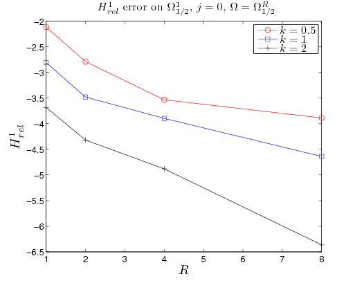
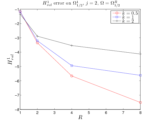
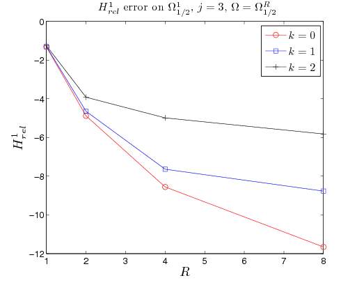
Figure 1: Numerical errors (lin-log scale) on the domain $\Omega_{1/2}^{1}$ by varying the exterior radius $R$ of the domain $\Omega_{1/2}^{R}$.

Ellipses

The second case presented is relative to the domain $E_{1/2}^{R}=\mathcal{E}_{R}\backslash B_{1/2}$ where $\mathcal{E}_{R}$ is the ellipses of equation $x^{2}/(2R)^{2}+y^{2}/(R)^{2}=1$. The numerical simulations are performed up to $R=8$. We mention that, with respect to the previous case, the CGM method is slightly slower to reach the desired tolerance. In Tables 2 we report the errors on $\Omega^{1}_{1/2}$ and $E_{1/2}^{R}$ for $R=1,2,4,8$ (the $L^{2}_{rel},H^{1}_{rel}$ errors on $\Omega^{1}_{1/2}$ are also shown in Figs.2)a-f in lin-log scale).

			Constant index of refraction:					Constant index of refraction:
			Errors on $\Omega_{1/2}^{1}$ ($\cdot 10^{-1}$)					Errors on $E_{1/2}^{R}$($\cdot 10^{-1}$)
$j$	$k$	$R$	$L^{2}$	$L^{2}_{rel}$	$H^{1}$	$H^{1}_{rel}$	$\delta J_{rel}$	$L^{2}$	$L^{2}_{rel}$	$H^{1}$	$H^{1}_{rel}$	$\delta J_{rel}$
0	0.5	$1$	$0.572$	$0.435$	$1.781$	$1.04$	$2.11$	$1.27$	$0.711$	$2.31$	$1.03$	$2.39$
		$2$	$0.291$	$0.221$	$0.902$	$0.528$	$0.966$	$2.24$	$0.761$	$2.646$	$0.751$	$0.516$
		$4$	$0.142$	$0.108$	$0.441$	$0.258$	$0.49$	$2.27$	$0.503$	$2.51$	$0.478$	$0.011$
		$8$	$0.0798$	$0.0607$	$0.245$	$0.144$	$0.581$	$1.54$	$0.232$	$1.731$	$0.229$	$0.0098$
0	1	$1$	$0.382$	$0.296$	$1.19$	$0.574$	$2.78$	$0.0807$	$0.0467$	$1.55$	$0.576$	$0.721$
		$2$	$0.179$	$0.139$	$0.553$	$0.265$	$1.15$	$1.061$	$0.379$	$1.45$	$0.345$	$0.12$
		$4$	$0.0905$	$0.0701$	$0.275$	$0.132$	$0.641$	$0.671$	$0.159$	$0.967$	$0.156$	$0.095$
		$8$	$0.0496$	$0.0384$	$0.151$	$0.0726$	$0.231$	$0.549$	$0.0881$	$0.76$	$0.0863$	$0.052$
0	2	$1$	$0.219$	$0.172$	$0.689$	$0.225$	$0.432$	$0.405$	$0.241$	$0.944$	$0.237$	$0.192$
		$2$	$0.115$	$0.0907$	$0.342$	$0.112$	$0.211$	$0.332$	$0.122$	$0.749$	$0.119$	$0.0921$
		$4$	$0.0585$	$0.0461$	$0.173$	$0.0523$	$0.115$	$0.249$	$0.0611$	$0.559$	$0.0603$	$0.0531$
		$8$	$0.00601$	$0.00474$	$0.00178$	$0.00582$	$0.0371$	$0.045$	$0.00772$	$0.101$	$0.0076$	$0.00821$
2	0.5	$1$	$1.282$	$2.232$	$5.12$	$2.051$	$0.449$	$2.18$	$3.71$	$6.42$	$2.53$	$0.252$
		$2$	$0.161$	$0.292$	$0.548$	$0.221$	$0.0541$	$1.52$	$2.35$	$2.37$	$0.921$	$0.0471$
		$4$	$0.0239$	$0.0435$	$0.0795$	$0.0321$	$0.00249$	$1.25$	$1.81$	$1.51$	$0.579$	$0.0131$
		$8$	$0.00964$	$0.0175$	$0.0305$	$0.0123$	$0.00125$	$0.715$	$0.991$	$0.794$	$0.303$	$0.0032$
2	1	$1$	$1.27$	$2.21$	$5.05$	$2.05$	$0.525$	$2.21$	$3.47$	$6.45$	$2.54$	$0.411$
		$2$	$0.0186$	$0.324$	$0.679$	$0.275$	$0.072$	$1.97$	$2.61$	$3.31$	$1.25$	$0.145$
		$4$	$0.0371$	$0.0658$	$0.133$	$0.0541$	$0.0211$	$0.844$	$0.951$	$1.17$	$0.432$	$0.0621$
		$8$	$0.0261$	$0.0451$	$0.0921$	$0.0372$	$0.00925$	$0.842$	$0.775$	$1.09$	$0.32$	$0.0211$
2	2	$1$	$1.14$	$1.73$	$4.51$	$1.78$	$0.634$	$2.04$	$2.54$	$6.22$	$2.25$	$0.757$
		$2$	$0.325$	$0.491$	$1.24$	$0.492$	$0.0211$	$1.76$	$1.58$	$3.81$	$1.16$	$0.301$
		$4$	$0.168$	$0.253$	$0.636$	$0.251$	$0.0132$	$1.19$	$0.781$	$2.66$	$0.652$	$0.122$
		$8$	$0.00182$	$0.00275$	$0.00711$	$0.00279$	$0.0026$	$0.0291$	$0.0141$	$0.0661$	$0.0127$	$0.0089$
3	0.5	$1$	$0.942$	$2.18$	$4.51$	$1.46$	$0.0831$	$1.44$	$3.28$	$5.83$	$1.83$	$0.0431$
		$2$	$0.0361$	$0.0841$	$0.127$	$0.0412$	$0.00354$	$0.394$	$0.884$	$0.729$	$0.235$	$0.00211$
		$4$	$0.00251$	$0.00581$	$0.00849$	$0.00272$	$0.00249$	$0.145$	$0.326$	$0.178$	$0.0575$	$0.000221$
		$8$	$0.000482$	$0.00112$	$0.00163$	$0.00053$	$0.00000647$	$0.0895$	$0.201$	$0.101$	$0.0324$	$0.0000921$
3	1	$1$	$0.887$	$2.02$	$4.19$	$1.36$	$0.141$	$1.42$	$3.18$	$5.57$	$1.81$	$0.0312$
		$2$	$0.0584$	$0.133$	$0.217$	$0.0707$	$0.0112$	$0.774$	$1.68$	$1.56$	$0.503$	$0.00778$
		$4$	$0.00471$	$0.0107$	$0.0168$	$0.0054$	$0.00127$	$0.281$	$0.603$	$0.394$	$0.126$	$0.00197$
		$8$	$0.00265$	$0.00605$	$0.00921$	$0.00299$	$0.000201$	$0.185$	$0.392$	$0.258$	$0.0831$	$0.000705$
3	2	$1$	$1.02$	$2.16$	$4.98$	$1.62$	$0.321$	$1.82$	$3.64$	$7.03$	$2.25$	$0.239$
		$2$	$1.04$	$0.221$	$0.461$	$0.151$	$0.0201$	$1.17$	$2.09$	$2.71$	$0.851$	$0.0941$
		$4$	$0.0415$	$0.0878$	$0.178$	$0.0581$	$0.00201$	$0.638$	$1.07$	$1.41$	$0.431$	$0.0301$
		$8$	$0.000811$	$0.0171$	$0.0272$	$0.000881$	$0.00000286$	$0.0178$	$0.0237$	$0.0401$	$0.0118$	$0.00168$

Table 2: The $L^{2},L^{2}_{rel},H^{1}_{rel},\delta J_{rel}$ errors of the numerical solution on $\Omega_{1/2}^{1}$ and $E_{1/2}^{R}$ by varying the semi-minor axis $R$ of $E_{1/2}^{R}$ for the case $j=0,2,3,k=0.5,1,2$.

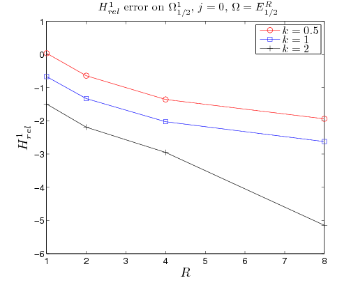
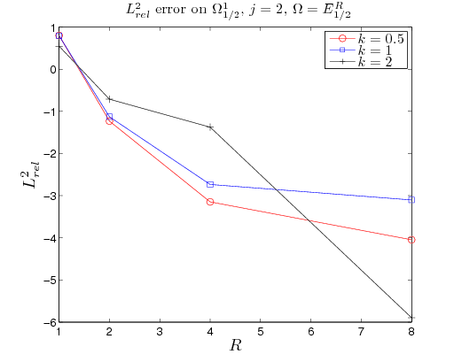
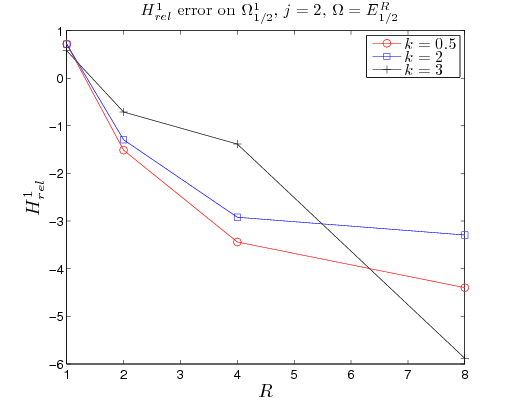
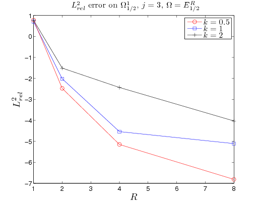
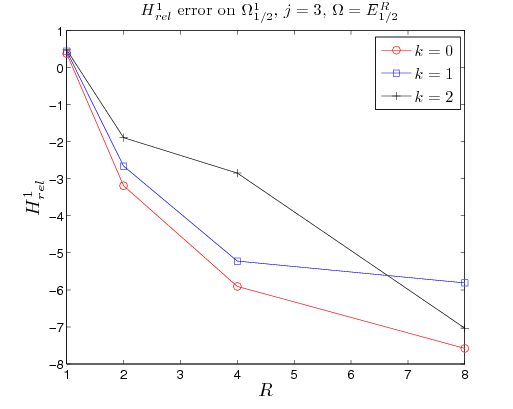
Figure 2: Numerical errors (lin-log scale) on the domain $\Omega_{1/2}^{1}$ by varying the semi-minor axis $R$ of $E_{1/2}^{R}$.

Squares

We conclude this section by showing a numerical investigation on the domain $S_{1/2}^{R}=Q_{R}\backslash B_{1/2}$ where $Q_{R}$ is the square centered in (0,0) and length side $2R$. The numerical simulations are performed up to $R=8$. Even if our approach can be applied to any domain, we mention that the presence of corners or edges deteriorate the convergence properties of the CGM method, at least if compared to the case in which the artificial boundary is regular (circle or ellipses). We also notice that imposing the Dirichlet boundary condition on the problem P1 (i.e. $C_{D}=1,C_{N}=0$) gives rise to a relevant oscillatory behavior of the solution near the corners due to the lack of regularity of the domain, while Neumann boundary gives a more regular behavior in the numerical solution. In Tables 3 we report the errors on $\Omega^{1}_{1/2}$ and $S_{1/2}^{R}$ by varying the semi-length side $R$ of $Q_{R}$ for $R=1,2,4,8$ (the $L^{2}_{rel},H^{1}_{rel}$ errors on $\Omega^{1}_{1/2}$ are also shown in Figs.3)a-f in lin-log scale).

			Constant index of refraction:					Constant index of refraction:
			Errors on $\Omega_{1/2}^{1}$ ($\cdot 10^{-1}$)					Errors on $S_{1/2}^{R}$($\cdot 10^{-1}$)
$j$	$k$	$R$	$L^{2}$	$L^{2}_{rel}$	$H^{1}$	$H^{1}_{rel}$	$\delta J_{rel}$	$L^{2}$	$L^{2}_{rel}$	$H^{1}$	$H^{1}_{rel}$	$\delta J_{rel}$
0	0.5	$1$	0.631	0.481	1.95	1.14	2.81	0.879	0.594	2.14	1.13	2.82
		$2$	0.321	0.243	0.986	0.577	0.571	1.84	0.717	2.269	0.727	0.645
		$4$	0.153	0.116	0.471	0.276	0.231	2.07	0.516	2.22	0.476	0.0810
		$8$	0.101	0.0771	0.312	0.182	0.0721	1.65	0.278	1.88	0.277	0.0451
0	1	$1$	0.0421	0.327	1.302	0.625	0.806	0.581	0.402	1.431	0.621	1.01
		$2$	0.197	0.153	0.603	0.289	0.606	0.944	0.381	1.23	0.331	0.606
		$4$	0.129	0.101	3.93	0.181	0.431	0.701	0.201	1.181	0.212	0.0151
		$8$	0.0467	0.0362	0.142	0.0681	0.0832	0.489	0.0881	0.684	0.0854	0.00521
0	2	$1$	0.241	0.188	0.729	0.238	1.935	0.317	0.223	0.798	0.235	0.0254
		$2$	0.139	0.109	0.411	0.134	0.851	0.336	0.141	0.798	0.143	0.0105
		$4$	0.0497	0.0391	0.146	0.0479	0.321	0.207	0.0561	0.473	0.0571	0.0526
		$8$	0.0320	0.0251	0.03942	0.0308	0.0851	0.176	0.0332	0.395	0.0322	0.0212
2	0.5	$1$	1.745	3.17	7.26	2.92	0.594	2.01	3.59	8.53	3.41	0.0297
		$2$	0.193	0.351	0.799	0.322	0.143	1.91	3.02	3.96	1.53	0.0143
		$4$	0.0192	0.0351	0.0796	0.0321	0.0675	1.25	1.88	1.65	0.636	0.00954
		$8$	0.00315	0.00572	0.0131	0.00525	0.0016	0.695	0.993	0.764	0.293	0.00438
2	1	$1$	1.73	3.07	7.14	2.89	0.681	1.98	3.39	8.39	3.35	0.129
		$2$	0.227	0.394	0.931	0.377	0.149	1.94	2.74	3.91	1.491	0.105
		$4$	0.0415	0.072	0.171	0.0691	0.0133	1.22	1.48	1.66	0.618	0.0441
		$8$	0.0141	0.0245	0.0578	0.0234	0.0079	0.654	0.663	0.904	0.323	0.014
2	2	$1$	1.51	2.37	6.25	2.47	0.912	1.76	2.587	7.08	2.71	0.574
		$2$	0.344	0.52	1.365	0.539	0.0624	1.62	1.67	3.37	1.10	0.355
		$4$	0.139	0.211	0.553	0.218	0.0144	1.02	0.771	2.19	0.59	0.125
		$8$	0.0961	0.144	0.381	0.151	0.0852	0.891	0.492	2.01	0.435	0.0788
3	0.5	$1$	1.17	2.71	6.13	1.99	0.97	1.63	3.75	7.56	2.45	0.107
		$2$	0.0422	0.0981	0.188	0.0611	0.0132	0.704	1.58	1.69	0.546	0.00874
		$4$	0.00237	0.00551	0.00861	0.00279	0.00292	0.247	0.554	0.393	0.115	0.000123
		$8$	0.000191	0.000445	0.000664	0.000216	0.000112	0.0962	0.215	0.109	0.0351	0.0000232
3	1	$1$	1.21	2.76	6.31	2.05	0.148	1.69	3.81	7.76	2.51	0.042
		$2$	0.0504	0.115	0.234	0.0761	0.0201	0.824	1.81	1.92	0.621	0.00602
		$4$	0.00304	0.00695	0.0137	0.00445	0.00986	0.356	0.771	0.521	0.167	0.00281
		$8$	0.00108	0.00246	0.00437	0.00142	0.000146	0.172	0.367	0.241	0.0777	0.000712
3	2	$1$	0.541	1.14	2.73	0.891	0.337	0.929	1.91	3.42	1.21	0.331
		$2$	0.0988	0.208	0.497	0.162	0.0401	1.12	2.07	2.63	0.833	0.105
		$4$	0.0276	0.0583	0.138	0.0451	0.000102	0.501	0.931	1.25	0.392	0.189
		$8$	0.0187	0.0396	0.0923	0.0301	0.000405	0.478	0.673	1.07	0.323	0.00782

Table 3: The $L^{2},L^{2}_{rel},H^{1}_{rel},\delta J_{rel}$ errors of the numerical solution on $\Omega_{1/2}^{1}$ and $S_{1/2}^{R}$ by varying the semi-lenght side $R$ of $S_{1/2}^{R}$ for the case $j=0,2,3,k=0.5,1,2$.

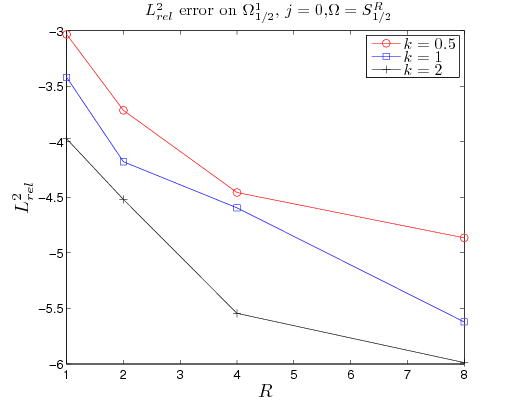
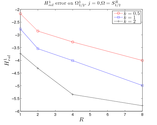
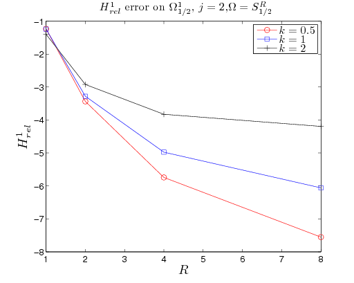
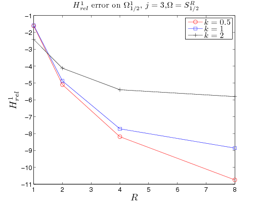
Figure 3: Numerical errors (lin-log scale) on the domain $\Omega_{1/2}^{1}$ by varying the semi-minor axis $R$ of $E_{1/2}^{R}$.

4 Numerical results for a variable index of refraction

In this section we apply our approach to cases of variable indices of refraction, for which an exact solution is not generally given. We notice that most of the numerical methods available in literature can be of difficult application, since they usually need the knowledge of the exact solution in some exterior domain. We also mention that the perfectly matched layer might be of nontrivial implementation when the material is not an analytic function in the direction perpendicular to the boundary, see [24],[28].

We stress that for a variable index of refraction it can be hard to compute the asymptotic behavior of the integrand function in (8) and, unlike the case of constant index of refraction, the weight $(1+|x|)^{-1}$ in the integral (10) has to be maintained.

Thus, given the same notation as the previous section, we are solving the following problem: to find $f\in L^{2}(\partial\Omega)$ such that the solution $u_{\Omega}[f]$ of

$$\begin{cases}\Delta u_{\Omega}[f]+k^{2}n(x)^{2}u_{\Omega}[f]=0,\qquad\textmd{in }\Omega\backslash B_{\hat{r}}\\ u_{\Omega}[f]=g,\quad\textmd{on }\partial B_{\hat{r}}\\ \partial_{\nu}u_{\Omega}[f]=f,\quad\textmd{on }\partial\Omega,\end{cases}$$

minimizes the integral

$$J(u_{\Omega}[f])=\int\limits_{\Omega\backslash B_{\hat{r}}}\Big{|}\nabla u_{\Omega}[f](x)-ikn(x)u_{\Omega}[f](x)\frac{x}{|x|}\Big{|}^{2}\frac{1}{1+|x|}dx.$$ (34)

In the following paragraphs we shall propose two indexes of refraction, namely

$$n_{1}(x,y) = 2+(\exp(-(x-1)^{2}-y^{2})+\exp(-(x+1)^{2}-y^{2}))\frac{x}{\sqrt{x^{2}+y^{2}}},$$

$$n_{2}^{a}(x,y) = 2+a\frac{x}{\sqrt{x^{2}+y^{2}}},$$

being $a$ a non negative real number. These indexes are shown in Figs.4a-b, with $a=0.1$. We stress that $n_{1}$ has an exponential decay to 2 at infinity and that $n_{2}^{a}$ it is not constant at infinity. For both cases, the geometry of the computational domain is the annulus $\Omega_{1/2}^{R}=B_{R}\backslash B_{1/2}$ for which a better convergence rate is achieved in the CGM algorithm, as seen in the previous section for a constant index of refraction.

Being an exact solution not available, we test the convergence properties as follows: we set the solution for $R=16$ as the reference one, and we shall compute the error norms up to $R=8$ as done in the previous sections. We always consider $j=0,k=1$.

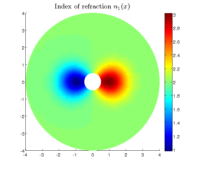
(a) $n_{1}(x,y)$

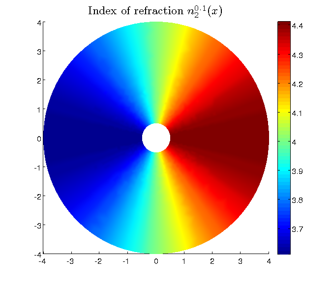
(b) $n_{2}^{0.1}(x,y)$

Figure 4: The indexes of refraction $n_{1}$ and $n_{2}^{a}$.

We notice that the choice of the functional (34) is appropriate only when the index of refraction does not generate guided modes (trapped waves). Due to the exponential decay at infinity, this requirement is satisfied by $n_{1}$ (see [1] and [31]). Regarding the index $n_{2}^{a}$ it is known from [29] that there is a critical value $a^{gm}$ according to which no guided modes are generated for $a\leq a^{gm}$. It is not easy to give a quantitative estimate of $a^{gm}$. By evaluating the integral (34) for several values of $a$ (see Fig.5 where the integral is shown at various exterior radius $R$ in log-lin scale), it seems that for $a\gtrapprox 0.6$ the integral diverge as $R\rightarrow\infty$. This suggests to consider $a\lessapprox 0.6$ for which it appears that the functional is bounded as $R\to\infty$. The numerical results for $n_{2}^{a}$ are therefore shown only for the small value $a=0.1$: if we are luckily in the case in which no guided modes are generated, our approach works well and the numerical solution converges to the exact one. More accurate estimates on $a^{gm}$ will be the object of future work.

Figure 5: The integral value $J(u_{\Omega_{1/2}^{R}[f]})$, by varying the exterior radius $R$ for various $a$ (log-lin scale): for $a\gtrapprox 0.6$ a likely numerical divergence is noticeable.

Case $n_{1}(x)$:

In Tables 4 we report the errors on $\Omega^{1}_{1/2}$ and $\Omega_{1/2}^{R}$ for $R=1,2,4,8$, (the $L^{2}_{rel},H^{1}_{rel}$ errors on $\Omega^{1}_{1/2}$ are also shown in Fig.7)a) in lin-log scale. In Figs.6a-b the real and imaginary parts of the numerical solution $u_{\Omega_{1/2}^{R}}[f]$ are shown for $R=16$

			Variable index of refraction $n_{1}(x)$:					Variable index of refraction $n_{1}(x)$:
			Errors on $\Omega_{1/2}^{1}$ ($\cdot 10^{-1}$)					Errors on $\Omega_{1/2}^{R}$ ($\cdot 10^{-1}$)
$j$	$k$	$R$	$L^{2}$	$L^{2}_{rel}$	$H^{1}$	$H^{1}_{rel}$	$\delta J_{rel}$	$L^{2}$	$L^{2}_{rel}$	$H^{1}$	$H^{1}_{rel}$	$\delta J_{rel}$
0	1	$1$	$0.734$	$0.582$	$2.85$	$1.01$	$0.088$
		$2$	$0.284$	$0.225$	$1.12$	$0.403$	$0.156$	$1.21$	$0.559$	$1.93$	$0.499$	$0.672$
		$4$	$0.174$	$0.137$	$0.502$	$0.177$	$0.0511$	$0.821$	$0.242$	$1.49$	$0.229$	$0.157$
		$8$	$0.0656$	$0.0521$	$0.203$	$0.0728$	$0.00602$	$0.411$	$0.0826$	$0.791$	$0.0842$	$0.00193$

Table 4: The $L^{2},L^{2}_{rel},H^{1}_{rel},\delta J_{rel}$ errors of the numerical solution on the annulus $\Omega_{1/2}^{1}$ and $\Omega_{1/2}^{R}$ by varying the exterior radius $R$ of the annular domain $\Omega_{1/2}^{R}$ for the variable index of refraction $n_{1}(x)=2+(\exp(-(x-1)^{2}-y^{2})+\exp(-(x+1)^{2}-y^{2}))\cos(\theta)$.

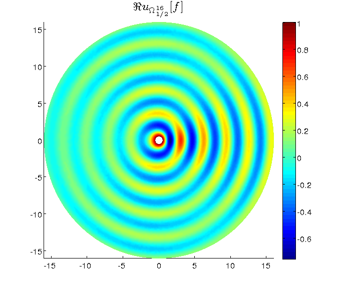
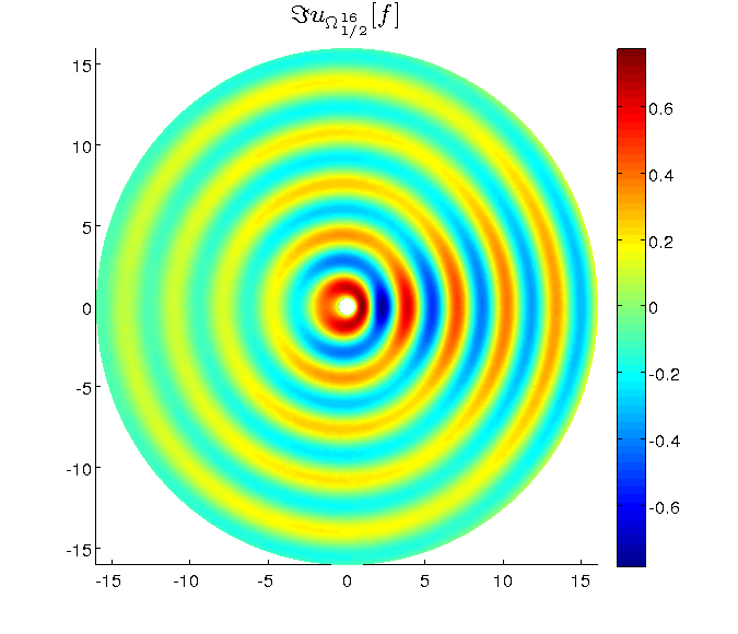
Figure 6: The real and imaginary parts of the numerical solution $u_{\Omega_{1/2}^{16}}$,index of refraction $n_{1}(x,y)$.

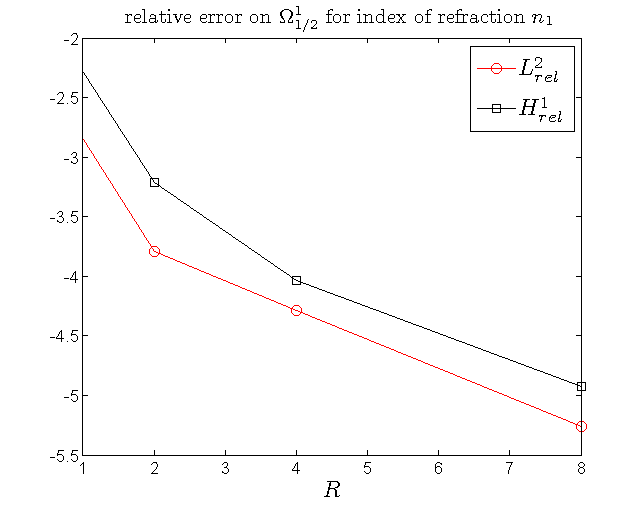
Figure 7: Numerical errors (lin-log scale) of the solution for variable index of refraction $n_{1}$ on the domain $\Omega_{1/2}^{1}$ by varying the radious $R$ of $\Omega_{1/2}^{R}$.

Case $n_{2}^{0.1}(x)$:

In Tables 5 we report the errors on $\Omega^{1}_{1/2}$ and $\Omega_{1/2}^{R}$ for $R=1,2,4,8$ (the $L^{2}_{rel},H^{1}_{rel}$ errors on $\Omega^{1}_{1/2}$ are also shown in Fig.9)b) in lin-log scale. In Figs.8a-b the real and imaginary parts of the numerical solution $u_{\Omega_{1/2}^{R}}[f]$ are shown for $R=16$.

			Variable index of refraction $n_{2}^{0.1}(x)$:					Variable index of refraction $n_{2}^{0.1}(x)$:
			Errors on $\Omega_{1/2}^{1}$ ($\cdot 10^{-1}$)					Errors on $\Omega_{1/2}^{R}$ ($\cdot 10^{-1}$)
$j$	$k$	$R$	$L^{2}$	$L^{2}_{rel}$	$H^{1}$	$H^{1}_{rel}$	$\delta J_{rel}$	$L^{2}$	$L^{2}_{rel}$	$H^{1}$	$H^{1}_{rel}$	$\delta J_{rel}$
0	1	$1$	0.522	0.408	1.65	0.582	0.826
		$2$	0.221	0.179	0.715	0.249	0.442	0.531	0.237	1.03	0.238	0.0925
		$4$	0.121	0.0951	0.402	0.141	0.273	0.421	0.122	0.0801	0.128	0.0833
		$8$	0.0872	0.0681	0.245	0.0861	0.168	0.478	0.0951	0.911	0.101	0.0161

Table 5: The $L^{2},L^{2}_{rel},H^{1}_{rel},\delta J_{rel}$ errors of the numerical solution on the annulus $\Omega_{1/2}^{1}$ and $\Omega_{1/2}^{R}$ by varying the exterior radius $R$ of the annular domain $\Omega_{1/2}^{R}$ for the variable index of refraction $n_{2}^{0.1}(x)=2+0.1\cos(\theta)$

(a) $n_{2}^{0.1}(x,y)$

(b) $n_{2}^{0.1}(x,y)$

Figure 8: The real and imaginary parts of the numerical solution $u_{\Omega_{1/2}^{16}}$, index of refraction $n_{2}^{0.1}(x,y)$.

Figure 9: Numerical errors (lin-log scale) of the solution for variable index of refraction $n_{2}^{0.1}$ on the domain $\Omega_{1/2}^{1}$ by varying the radious $R$ of $\Omega_{1/2}^{R}$.

Conclusions

We studied a new approach to the problem of transparent boundary conditions for the Helmholtz equation. Our method is based on the minimization of an integral functional which arises from a volume integral formulation of the Sommerfeld radiation condition. When the artificial domain is a ball, we proved analytical results on the convergence of the approximate solution to the exact one under quite general assumptions on the index of refraction. We tested numerically our method for a constant index of refraction by choosing three shapes of the artificial boundary in $\mathbb{R}^{2}$: a ball, an ellipse and a square. The convergence results are satisfactory; in particular we observed a good convergence rate for the $H^{1}_{rel}$ norm. We also applied our approach to other indices of refraction, one exponentially decaying at infinity to a constant, and one not constant at infinity.

Since our approach is of easy implementation and has wide application, we believe that it can be a good starting point for studying problems with nontrivial indices of refraction. However, when the index of refraction is constant, the methods available in literature are more suitable. We stress that numerical results show that our approach do not suffer the choice of the shape of the artificial domain.

Our approach applies also to more general settings. In particular, we have in mind the waveguide problem. In this case, the functional $J$ has to be modified on account of the presence of guided modes (see [2],[9]-[12]); this will be the object of future work.

References

[1] S. Agmon, Spectral properties of Schrödinger operators and scattering theory. Ann. Sc. Norm. Sup. Pisa Ser., 4 2 (1975), 121–218.
[2] O. Alexandrov and G. Ciraolo. Wave propagation in a 3-D optical waveguide. Math. Models Methods Appl. Sci. (M3AS), 14 (2004), no.6, 819–852.
[3] R.J. Astley, Infinite elements for wave problems: a review of current formulations and an assessment of accuracy, Int. J. Numer.
Methods Engrg., 49 (2000), 951–976.
[4] C. Atamian, Q.V. Dinh, R. Glowinski, J. He, J. Periaux Control approach to fictitious domain methods: Applications to fluid dynamics and electromagnetics.
Proc. Fourth Int. Conf. on Domain Decomposition Methods for Partial Differential Equations, SIAM, Philadelphia (1991), pp. 275–309.
[5] P. Bettess, Infinite elements, Int. J. Numer. Methods Engrg., 11 (1977), 53–64.
[6] P. Bettess, Infinite Elements, Penshaw Press, Sunderland, UK, 1992.
[7] J.-P. Bérenger, A perfectly matched layer for the absorption of electromagnetic waves, J. Comput. Phys. 114 (1994), 185–200.
[8] A. Bayliss and E. Turkel, Radiation boundary conditions for wave-like equations, Comm. Pure Appl. Math., 33 (1980), 707–725.
[9] G. Ciraolo, A method of variation of boundaries for waveguide grating couplers, Applicable Analysis, 87 (2008), 1019–1040.
[10] G. Ciraolo, A radiation condition for the 2-D Helmholtz equation in stratified media, Comm. Part. Diff. Eq., 34 (2009), 1592–1606.
[11] G. Ciraolo and R. Magnanini. Analytical results for 2-D non-rectilinear waveguides based on the Green’s function. Math. Methods Appl. Sci., 31 (2008), no.13, 1587–1606.
[12] G. Ciraolo and R. Magnanini, A radiation condition for uniqueness in a wave propagation problem for 2-D open waveguides, Math. Methods Appl. Sci., 32 (2009), 1183–1206.
[13] D. Colton and R. Kress, Inverse Acoustic and Electromagnetic Scattering Theory, Springer-Verlag Berlin, Heidelberg, New York, 1992.
[14] B. Engquist and A. Majda, Radiation boundary conditions for acoustic and elestic wave calculations, Comm. Pure Appl. Math., 32 (1979), 314–358.
[15] D. Givoli and J.B. Keller, A finite element method for large domains, Comput. Methods Appl. Mech. Engrg., 76 (1989), 41–66.
[16] D. Givoli, Numerical Methods for Problems in Infinite Domains. Studies in Applied Mechanics, vol. 33, Elsevier Scientific. Publishing Co., Amsterdam, 1992.
[17] D. Givoli, Exact representations on artificial interfaces and applications in mechanics, AMR, 52 (1999), 333–349.
[18] D. Givoli, Recent advances in the DtN FE method, Arch. Comput. Methods Engrg., 6 (1999), 71–116.
[19] D. Givoli, High-order local non-reflecting boundary conditions: a review, Wave motion, 39 (2004), 319–326.
[20] M.J. Grote and J.B. Keller, On nonreflecting boundary conditions, J. Comput. Phys., 122 (1995), 231–243.
[21] T. Hagstrom, Radiation boundary conditions for the numerical simulation of waves, Acta Numer., 8 (1999), 47–106.
[22] I. Harari, A survey of finite element methods for time-harmonic acoustics, Comput. Methods Appl. Mech. Engrg., 195 (2006), 1594–1607.
[23] F. Ihlenburg, Finite Element Analysis of Acoustic Scattering, Springer-Verlag, New York, 1998.
[24] S.G. Johnson, Notes on perfectly matched layers (PMLs). Massachusetts Institute of Technology, Technical Report, 2007; updated 2010. Available at:http://www-math.mit.edu/ stevenj/18.369/pml.pdf.
[25] J.B. Keller and D. Givoli, Exact nonreflecting boundary conditions, J. Comput. Phys., 82 (1989), 172–192.
[26] R. Leis, Initial Boundary Value Problems in Mathematical Physics, J. Wiley & Teubner Verlag, Stuttgart, 1986.
[27] M. Medvinsky, E. Turkel, U. Hetmaniuk, Local absorbing boundary conditions for elliptical shaped boundaries.
J. Comput. Phys. 227 (2008), no. 18, 8254–8267.
[28] A.F. Oskooi, L. Zhang, Y. Avniel, S.G. Johnson, The failure of perfectly matched layers, and towards their redemption by adiabatic absorbers. Opt. Express, 16 (15) (2008), pp. 11376–11392.
[29] B. Perthame and L. Vega, Energy concentration and Sommerfeld condition for Helmholtz equation with
variable index at infinity, GAFA Geom. Funct. Anal., 17 (2008), 1685–1707.
[30] F. Rellich, Über das asymptotische Verhalten del Lösungen von in unendlichen
Gebieten, Jber. Deutsch. Math. Verein., 53 (1943), 57 – 65.
[31] Y. Saito, Spectral and scattering theory for second-order differential operators
with operator-valued coefficients, Osaka J. Math. 9 (1972), 463–498.
[32] Y. Saito, Schrödinger operators with a nonspherical radiation condition, Pacif. J. of Math., 126 (1987), 331–359.
[33] S. A. Sauter and C. Schwab. Boundary element methods. Springer Series in Computational Mathematics, 39. Springer-Verlag, Berlin, 2011.
[34] S.V. Tsynkov, Numerical solution of problems on unbounded domains. A review, Appl. Numer. Math., 27 (1998), 465–532.
[35] E. Turkel and A. Yefet, Absorbing PML boundary layers for wave-like equations, Appl. Numer. Math. 27 (1998), 533–557.
[36] M. Zubeldia, Energy concentration and explicit Sommerfeld radiation condition for the electromagnetic Helmholtz equation, preprint 2012, arXiv:1201.0494.