Self-heating in kinematically complex magnetohydrodynamic flows

Abstract

The non-modal self-heating mechanism driven by the velocity shear in kinematically complex magnetohydrodynamic (MHD) plasma flows is considered. The study is based on the full set of MHD equations including dissipative terms. The equations are linearized and unstable modes in the flow are looked for. Two different cases are specified and studied: (a) the instability related to an exponential evolution of the wave vector; and (b) the parametric instability, which takes place when the components of the wave vector evolve in time periodically. By examining the dissipative terms, it is shown that the self-heating rate provided by viscous damping is of the same order of magnitude as that due to the magnetic resistivity. It is found that the heating efficiency of the exponential instability is higher than that of the parametric instability.

I Introduction

It is widely known that astrophysical, terrestrial and laboratory plasma flows are most often characterized by spatially inhomogeneous velocities, constituting so-called shear flows. In many cases, these flows are kinematically complex, multidimensional and sometimes they are also relativistic. Among the different kinds of plasma shear flows many exhibit motion profiles with highly nontrivial velocity fields. One prominent class of such flows contains the swirling astrophysical flows that until now have received only little theoretical attention. In particular, many galaxies reveal relativistic jets tavec , some of which are characterized by helical motion patterns broder ; kharb . A similar situation is met in pulsars, where morphological and spectroscopic studies make strong jet-like structures evident crabjet ; pjet1 . Even closer to us, namely in the solar atmosphere, the existence of giant macro-spicules featuring swirling, tornado-like plasma motions has been reported pm98 .

The latter class of jet-like large-scale velocity patterns in the atmosphere of the Sun deserves some special attention. In 1991, the Yohkoh Solar Observatory detected coronal jets (by means of the Soft X-Ray Telescope tsun ) which were assumed to be related to evaporation flows shimo . More recently, it has been reported on the ³He-rich solar energetic particle event sjet observed on 2006 November $18\,$th by the X-Ray Telescope on board the Hinode satellite golub . There is also some indirect observational evidence for the presence of more complicated velocity patterns. In particular, blue shifted and red shifted emission on either side of the axis of a macro-spicule has been reported pm98 . These observations were interpreted as indicating at the presence of a rotation within these tall pillars of hot and magnetized, swirling plasma flows. Another interesting class of astronomical objects with an observational evidence of swirling flows is the Herbig-Haro jets. It was shown that the young stellar object HH 212 exhibits strong indications for the presence of rotation in the jet davis . A similar helical structure is observed in DG Tau bacc .

Therefore, the study of kinematically complex shear flows with a non-trivial geometry is interesting and necessary because flow patterns with nontrivial velocity fields appear to be quite common in astrophysics. Besides, it seems reasonable to expect that the kinematic complexity could considerably influence the physical processes within these flows and lead to various detectable observational appearances in the related astronomical objects.

Recently, it was fully realized that collective phenomena in shear flows are characterized by so-called non-modal processes, related with non-normality tref . These processes are fairly well-understood for a variety of flows, see, for instance, rmb97 ; bod01b ; andro ; chven . In particular, in andro ; chven shear flow instabilities are studied in helical flows. The problem was considered both for the incompressible andro and compressible chven cases and it has been shown that shear flows efficiently amplify the fast/slow magnetosonic waves (in the case of compressible flows) and the Alfvén waves (in both cases). It was also argued that these instabilities may lead to so-called ’non-modal self-heating’. This process involves three major stages: (a) First, the waves are excited spontaneously within the shear flow; (b) second, the excited modes undergo a non-modal amplification, extracting a part of the equilibrium flow’s kinetic energy and (c) third, in the final stage, the non-modally amplified waves get dissipated via viscous damping and/or magnetic resistive diffusion and give their energy back to the background flow in the form of heat.

This mechanism was originally described in androSH for the case of a hydrodynamic flow and it has been argued that self-heating may play an important role also in the dynamics of kinematically complex magnetized flows. In lcl06 it has been shown that efficient non-modal self-heating can indeed take place in magnetized media as well. A direct application to the solar atmosphere was proposed in spp06 where it was concluded that self-heating could serve as an efficient mechanism for providing, or at least contributing to, the heat production in the lower corona. Recently, we have studied the efficiency of non-modal self-heating by acoustic wave perturbations in the solar chromosphere rop10 . It has been shown that amplified waves get damped due to the presence of viscous dissipation and indeed cause an energy transfer back to the background flow in the form of heat.

In most of the above cited papers, the problem of self-heating was considered only for shear flows with relatively simple flow geometry, while the flows occurring in astrophysical plasmas, as well as in many terrestrial and laboratory situations, can be significantly more complex. Therefore, it is quite timely and important to examine kinematically more complicated cases and verify if the mechanism is also efficient when such complex flow patterns occur. For this purpose, in the present paper we study the possibility of non-modal self-heating in fully compressible, kinematically complex MHD flows taking into account both viscosity and magnetic resistivity.

The paper is arranged in the following way. In section II, we formulate the model for the study of non-modal shear flow instabilities for MHD flows including resistive terms and we derive the equations governing the self-heating process. In section III, we apply our model to the fully compressible flows examining the high plasma-$\beta$ case and we then investigate numerically the efficiency of the self-heating mechanism. In section IV, we discuss the obtained results and outline the directions of further, more detailed, quantitative and applicative studies.

II Main Consideration

In order to study the self-heating mechanism in magnetized plasma flows, we start with the standard set of polytropic MHD equations consisting of the equation of mass conservation:

$$D_{t}\rho+\rho\nabla\cdot{\bf V}=0,$$ (1)

the momentum conservation equation:

$$D_{t}{\bf V}=-\frac{1}{\rho}{\bf\nabla P}-\frac{{\bf B}}{4\pi\rho}\times({\bf\nabla\times B})+\nu\Delta{\bf V},$$ (2)

the induction equation:

$$D_{t}{\bf B}=({\bf B}\cdot\nabla){\bf V}-{\bf B}(\nabla\cdot{\bf V})+\eta\Delta{\bf B},$$ (3)

Gauss’s law for magnetism:

$${\bf\nabla\cdot B}=0,$$ (4)

and the polytropic equation of state:

$$P=C{\rho}^{1+1/n},$$ (5)

where $D_{t}\equiv\partial_{t}+({\bf V}\cdot\nabla)$ denotes the convective derivative, $\rho$ is the density, $P$ stands for the pressure, ${\bf V}$ is the velocity field, ${\bf B}$ denotes the magnetic field, $\nu$ stands for the coefficient of kinematic viscosity, $\eta$ is the magnetic resistivity coefficient, and $C={\it const}$ and $n$ are the polytropic constant and the polytropic index, respectively. Note that in the framework of the present paper we consider a common stellar model, viz. the so-called “Polytropic Star Model” in which the pressure depends only on the density according to the polytropic equation of state, Eq. (5) carroll .

The equilibrium state of the model is specified by a homogeneous MHD plasma ($\rho_{0}=\hbox{\it const}$), embedded in a uniform, vertical magnetic field (${\bf B_{0}}\equiv[0,0,B_{0}=\hbox{\it const}]$). For analyzing the full set of MHD equations, we first linearize them, perturbing all physical quantities about the equilibrium state:

$$\rho\equiv\rho_{0}+\rho^{\prime},$$ (6)

$${\bf V}\equiv{\bf U}+{\bf v},$$ (7)

$${\bf B}\equiv{\bf B_{0}}+{\bf B^{\prime}},$$ (8)

and

$$P\equiv P_{0}+P^{\prime}.$$ (9)

It is assumed that the perturbations $\rho^{\prime}$, ${\bf v}$, ${\bf B^{\prime}}$ and $P^{\prime}$ are small compared to the corresponding equilibrium quantities, viz. $\rho_{0}$, ${\bf U}$, ${\bf B_{0}}$ and $P_{0}$, respectively. By substituting Eqs. (6-9) into Eqs. (1-5), and then linearizing (i.e. keeping only the first-order terms in the perturbed quantities), one can derive the following set of equations for the perturbed quantities:

$$\mathcal{D}_{t}D+{\bf\nabla}\cdot{\bf v}=0,$$ (10)

$$\mathcal{D}_{t}{\bf v}+({\bf v}\cdot\nabla){\bf U}=-C_{s}^{2}{\bf\nabla}D+C_{A}^{2}[\partial_{z}{\bf b}-{\bf\nabla}b_{z}]+\nu\Delta{\bf v},$$ (11)

$$\mathcal{D}_{t}{\bf b}=({\bf b\cdot\nabla)U}+\partial_{z}{\bf v}+{\bf e_{z}(\nabla\cdot v)}+\eta{\bf\Delta b},$$ (12)

$${\bf\nabla\cdot b}=0,$$ (13)

where $\mathcal{D}_{t}\equiv\partial_{t}+({\bf U}\cdot\nabla)$, $D\equiv\rho^{\prime}/\rho_{0}$, ${\bf b}\equiv{\bf B^{\prime}}/B_{0}$, $C_{s}=\sqrt{dP_{0}/d\rho_{0}}$ denotes the sound speed and $C_{A}\equiv B_{0}/\sqrt{4\pi\rho_{0}}$ is the Alfvén speed.

Following the method developed in mahand , we assume that ${\bf U}$ is a spatially inhomogeneous vector velocity field. We expand the velocity in Taylor series around a point $A(x_{0},y_{0},z_{0})$, preserving only the linear terms:

$${\bf U}={\bf U}(A)+\sum_{i=1}^{3}\frac{\partial{\bf U}(A)}{\partial x_{i}}(x_{i}-x_{i0}),$$ (14)

where $i=1,2,3$ and $x_{i}=(x,y,z)$.

Mahajan and Rogava have shown that by applying the following ansatz

$$F(x,y,z,t)\equiv\hat{F}(t)e^{\phi_{1}-\phi_{2}},$$ (15)

$$\phi_{1}\equiv\sum_{i=1}^{3}{K_{i}}(t)x_{i},$$ (16)

$$\phi_{2}\equiv\sum_{i=1}^{3}U_{i}(A)\int{K_{i}}(t)dt,$$ (17)

to Eqs. (10-11), these equations transform to a set of ordinary differential equations mahand . This reduces the problem mathematically to the study of an initial value problem. By $U_{i}(A)$ we denote the equilibrium velocity components and the $K_{i}(t)$ represent the wave number vector components satisfying the following set of differential equations mahand :

$${\bf\partial_{t}K}+{\bf S^{T}}\cdot{\bf K}=0,$$ (18)

where ${\bf S^{T}}$ is the transposed shear matrix. This shear matrix ${\bf S}$ is defined by:

$${\bf S}=\left(\begin{array}[]{ccc}U_{x,x}&U_{x,y}&U_{x,z}\\ U_{y,x}&U_{y,y}&U_{y,z}\\ U_{z,x}&U_{z,y}&U_{z,z}\\ \end{array}\right),$$ (19)

with $U_{i,k}\equiv\partial U_{i}/\partial x_{k}$.

Working with the background velocity field ${\bf U(r)}\equiv[0,r\Omega(r),U(r)]$, the shear matrix obtains the following form andro ; chven

$${\bf S}=\left(\begin{array}[]{ccc}\Sigma&A_{1}&0\\ A_{2}&-\Sigma&0\\ C_{1}&C_{2}&0\\ \end{array}\right).$$ (20)

By taking Eqs. (15-18,20) into account, the set of Eqs. (10-13) reduces to the following dimensionless form

$$d^{(1)}={\bf k}\cdot{\bf u},$$ (21)

$${\bf u}^{(1)}+{\bf s}\cdot{\bf u}=-{\bf k}\epsilon^{2}d+{\bf h}-{\bf k}h_{z}-\overline{\nu}k^{2}{\bf u},$$ (22)

$${\bf h}^{(1)}={\bf s\cdot h-u-e_{z}(k\cdot u)}-\overline{\eta}k^{2}{\bf h},$$ (23)

$${\bf k\cdot h}=0,$$ (24)

$$\textbf{k}^{(1)}+{\bf s^{T}}\cdot{\bf k}=0,$$ (25)

with

$${\bf s}=\left(\begin{array}[]{ccc}\sigma&a_{1}&0\\ a_{2}&-\sigma&0\\ r_{1}&r_{2}&0\\ \end{array}\right),$$ (26)

where $d\equiv iD$, ${\bf u}\equiv{\bf v}/C_{A}$, ${\bf h}\equiv i{\bf b}$, $\epsilon\equiv C_{s}/C_{A}$, $a_{1,2}\equiv A_{1,2}/K_{z}C_{A}$, $\sigma\equiv\Sigma/K_{z}C_{A}$, $r_{1,2}\equiv C_{1,2}/K_{z}C_{A}$, $\textbf{k}\equiv\textbf{K}/K_{z}$, $\overline{\nu}\equiv\nu K_{z}/C_{A}$ and $\overline{\eta}\equiv\eta K_{z}/C_{A}$. By $F^{(1)}$ we denote $dF/d\tau$ and $\tau\equiv K_{z}C_{A}t$ is the dimensionless time.

For estimating the efficiency of the self-heating mechanism, it is useful to define the total energy of the perturbations:

$$E_{tot}\equiv E_{kin}+E_{m}+E_{c}=\frac{{\bf u^{2}}}{2}+\frac{{\bf h^{2}}}{2}+\frac{{\epsilon^{2}d^{2}}}{2},$$ (27)

which consists of the kinetic, magnetic and compressional energies, respectively. The evolutionary equation for the total energy has the following form:

$$E^{(1)}_{tot}=-{\bf u(s\cdot u)}+{\bf h(s\cdot h)}-2h_{z}{\bf(k\cdot u)}-$$

$$\;\;\;\;\;\;\;\;\;\;\;\;\;\;\;\;\;\;\;\;\;\;\;\;\;\;\;\;\;\;\;\;\;\;\;\;\;\;\;\;\;\;\;\;\;\;\;\;\;\;-\overline{\nu}{\bf k^{2}u^{2}}-\overline{\eta}{\bf k^{2}h^{2}}.$$ (28)

As it is clear from Eq. (28), the last two (viscosity and magnetic resistivity) terms are responsible for the energy dissipation and thus for the final stage of the self-heating process. By means of these two terms one can define the so-called ’self-heating rate’, originally introduced in androSH only for purely hydrodynamic flows:

$$\Psi(\tau)\equiv\frac{1}{E_{tot}(0)}\int_{0}^{\tau}\left[\overline{\nu}{\bf k^{2}}(\tau^{\prime}){\bf u^{2}}(\tau^{\prime})+\overline{\eta}{\bf k^{2}}(\tau^{\prime}){\bf h^{2}}(\tau^{\prime})\right]d\tau^{\prime}.$$ (29)

III Discussion

In this section, we study the efficiency of the self-heating mechanism for different values of parameters, taking into account both the viscous damping and magnetic resistivity terms. Generally speaking, for the non-modal self-heating process to be efficient, the dissipative terms must not be too small in order to provide substantial heating. However, at the same time the damping should not be “too strong” either: non-modally amplified modes have to have enough time for growing and extracting the equilibrium flow energy before damping occurs. As it is clear from Eqs. (2-3), the effects of dissipation become important only for relatively small length scales.

Mathematically the non-modal instability is described by the system of equations (21-25), where Eq. (25) plays an important role. In particular, in plane-parallel flows ${\bf k}$ exhibits a linear time evolution rog00 , whereas for multidimensional cases (such as for helical flows), the components of the wave vector may evolve in time either exponentially or periodically andro ; chven . Linearly and exponentially evolving wave vectors lead to so-called ’usual’ instabilities (with $\Gamma^{2}\equiv\sigma^{2}+a_{1}a_{2}>0$). Parametrically unstable modes deserve a special interest. These modes appear for periodically evolving ${\bf k}$’s (i.e. $\Gamma^{2}<0$) for certain values of the parameters.

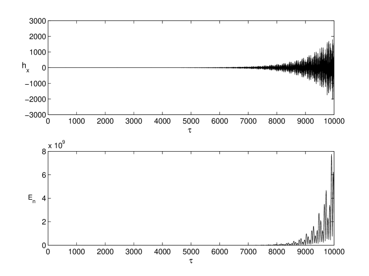
Figure 1: The temporal behavior of $h_{x}(\tau)$ and the energy $E_{n}(\tau)\equiv E_{tot}(\tau)/E_{tot}(0)$ normalized by its initial value for the following set of parameters: $\sigma=0$, $a_{1}=-a_{2}=-1$, $r_{1}=0.01$, $r_{2}=0.9406$, $\epsilon=0.1$, $k_{x0}=k_{y0}=10$, $u_{x0}=u_{y0}=u_{z0}=0$, $h_{x0}=0.01$, $h_{y0}=0$, $d_{0}=0$, $\overline{\nu}=\overline{\eta}=0$. Note that the range of $r_{2}$, where the evolution of the modes is parametrically unstable, is very narrow: $[0.94;0.941]$.

In Fig. 1, we show the temporal behavior of $h_{x}(\tau)$ and the energy $E_{n}(\tau)\equiv E_{tot}(\tau)/E_{tot}(0)$ normalized by its initial value. The considered set of parameters is: $\sigma=0$, $a_{1}=-a_{2}=-1$, $r_{1}=0.01$, $r_{2}=0.9406$, $\epsilon=0.1$, $k_{x0}=k_{y0}=10$, $u_{x0}=u_{y0}=u_{z0}=0$, $h_{x0}=0.01$, $h_{y0}=0$, $d_{0}=0$, $\overline{\nu}=\overline{\eta}=0$. As it is clear from the plots, despite $\Gamma^{2}<0$, the system exhibits unstable modes. The instability takes place only for very narrow ranges of parameters. In particular, one can straightforwardly check that the instability disappears for values of $r_{2}$ outside the interval $[0.94;0.941]$.

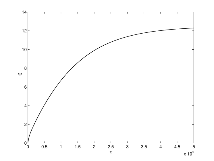
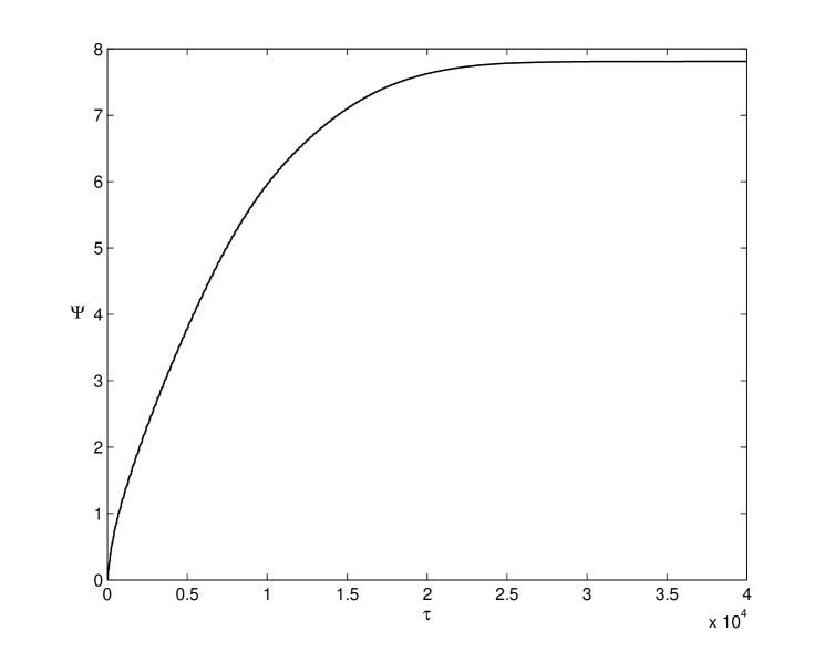
Figure 2: The temporal evolution of the self-heating rate for two different cases. Top panel: $\overline{\nu}=1.25\times 10^{-4}$, $\overline{\eta}=0$. Bottom panel: $\overline{\nu}=0$, $\overline{\eta}=1.25\times 10^{-4}$. The set of parameters is $\sigma=0$, $a_{1}=-a_{2}=-1$, $r_{1}=0.01$, $r_{2}=0.9406$, $\epsilon=0.1$, $k_{x0}=k_{y0}=10$, $u_{x0}=u_{y0}=u_{z0}=0$, $h_{x0}=0.01$, $h_{y0}=0$, $d_{0}=0$.

The dissipative factors will inevitably lead to the self-heating effect. In particular, Fig. 2 shows the temporal evolution of the self-heating rate for two different cases: on the top panel we examine $\overline{\nu}=1.25\times 10^{-4}$, $\overline{\eta}=0$ and on the bottom panel the result is shown for $\overline{\nu}=0$ and $\overline{\eta}=1.25\times 10^{-4}$. All the other parameters are the same as in Fig. 1. As we see from the plots, there is no principal difference between viscosity-dominated and magnetic-resistivity-dominated cases, i.e. the saturated values of the self-heating rates are of the same order of magnitudes. In both cases, the energy converted into heat exceeds the initial perturbation energy about 10 times. This means that the excited non-modal waves extract energy from the mean flow and this energy, via the agency of the dissipative terms, is converted into heat and given back to the flow. As we see from the results, the efficiency of the self-heating is quite high.

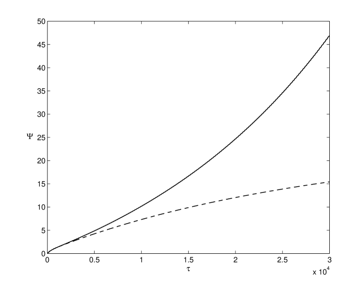
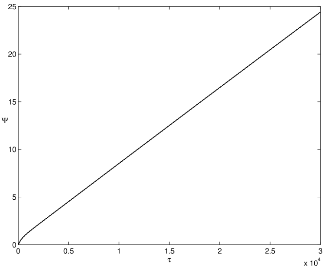
Figure 3: The temporal evolution of the self-heating rate for three different cases. Top panel: $\overline{\nu}=1.2\times 10^{-5}$ (solid line) and $\overline{\nu}=1.24\times 10^{-5}$ (dashed line). Bottom panel: $\overline{\nu}=1.22\times 10^{-5}$. The set of parameters is $\sigma=0$, $a_{1}=-a_{2}=-1$, $r_{1}=0.01$, $r_{2}=0.9406$, $\epsilon=0.1$, $k_{x0}=k_{y0}=10$, $u_{x0}=u_{y0}=u_{z0}=0$, $h_{x0}=0.01$, $h_{y0}=0$, $d_{0}=0$.

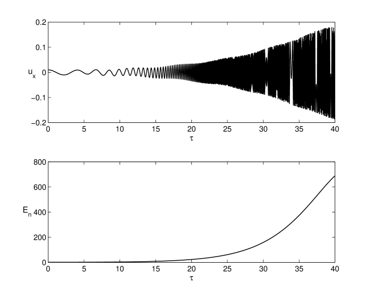
Figure 4: The temporal behavior of $u_{x}(\tau)$ and $E_{n}(\tau)$. The considered set of parameters is $\sigma=0$, $a_{1}=a_{2}=1$, $r_{1}=r_{2}=0$, $\epsilon=0.1$, $k_{x0}=1$, $k_{y0}=0$, $u_{x0}=0$, $u_{y0}=u_{z0}=0$, $h_{x0}=h_{y0}=0$, $d_{0}=0$, $\overline{\nu}=\overline{\eta}=0$.

It is worth noting that for the considered mechanism to be efficient, several conditions must be satisfied. At the one hand, the instability must be robust enough to provide an amplification of the waves and, additionally, the dissipation process must not be too efficient in order to avoid damping of the excited modes before they grow substantially enough. On the other hand, if the damping is too weak the amplified waves fail to give back their energy back to the flow. Therefore, one may expect that self-heating will be efficient for a limited range of moderatly dissipative systems.

On the top panel of Fig. 3, we show the temporal evolution of the self-heating rate for $\overline{\nu}=1.2\times 10^{-5}$ (solid line) and $\overline{\nu}=1.24\times 10^{-5}$ (dashed line). The other parameters are again the same as in Fig. 1. As it is evident from the plots, for the case presented by the solid line, the viscosity is not strong enough and non-modaly amplified modes avoid any significant viscous dissipation. In general, the temporal evolution of the self-heating rate is very sensitive to viscosity. By slightly increasing the value of the viscosity, the situation might change drastically. By the dashed line we show the result for $\overline{\nu}=1.24\times 10^{-5}$, and it is clear that unlike the previous case, more dominant viscous terms here ensure stronger self-heating. The efficiency of the instability seems significantly decreased and $\Psi(t)$ tends to become saturated (see Fig. 2). This tendency implies that for a certain value of the viscosity the effects of non-modal instability and dissipation will balance each other. This particular case is presented on the bottom panel of Fig. 3, where the value of the viscosity equals $1.22\times 10^{-5}$ and, as we see from the figure, the self-heating rate shows a linear dependence on time.

We have already noticed that apart from the parametric instability, the system under consideration exhibits also ‘usual’ instabilities ($\Gamma^{2}>0$), characterized by exponentially evolving wave number vector. Normally, in these cases the waves are more unstable than the parametrically unstable modes. In particular, in Fig. 4 we show the temporal behavior of $u_{x}(\tau)$ and $E_{n}(\tau)$. The considered set of parameters is: $\sigma=0$, $a_{1}=a_{2}=1$, $r_{1}=r_{2}=0$, $\epsilon=0.1$, $k_{x0}=1$, $k_{y0}=0$, $u_{x0}=0$, $u_{y0}=u_{z0}=0$, $h_{x0}=h_{y0}=0$, $d_{0}=0$, $\overline{\nu}=\overline{\eta}=0$. As we see from the figure, the energy perturbation and $u_{x}$ significantly increase until $\tau=40$. These results can be explained as follows: since $\Gamma^{2}>0$, the wave vector components evolve with time exponentially (unlike the cases presented by figures 1-3) and correspondingly, the system undergoes a strong instability, the growth rate of which exceeds that of the parametric instability. For the same reason, the efficiency of the self-heating mechanism for the unstable non-modal modes shown in Fig. 4 must be higher with respect to the self-heating rate for parametrically unstable waves.

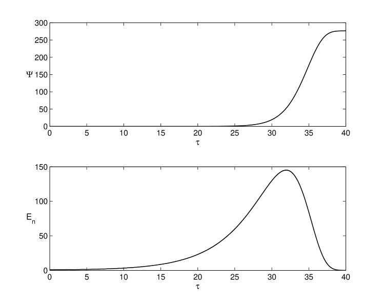
Figure 5: The temporal behavior of $\Psi(\tau)$ and $E_{n}(\tau)$. The considered set of parameters is $\sigma=0$, $a_{1}=a_{2}=1$, $r_{1}=r_{2}=0$, $\epsilon=0.1$, $k_{x0}=1$, $k_{y0}=0$, $u_{x0}=0$, $u_{y0}=u_{z0}=0$, $h_{x0}=h_{y0}=0$, $d_{0}=0$, $\overline{\nu}=1\times 10^{-5}$, $\overline{\eta}=0$.

In Fig. 5, we show the temporal evolution of $\Psi(\tau)$ and $E_{n}(\tau)$. The considered set of parameters is the same as in the previous figure, except for $\overline{\nu}=1\times 10^{-5}$. It is clear from the plots, that initially the instability rate exceeds that of the self-heating (negligible role of the dissipative factors), and therefore, the perturbation energy increases. In the course of time, due to the exponential growth of the wave vectors’ components, the effective length scale, $\lambda\sim 1/k$ decreases, leading to an increasing role of the viscous terms. As a result, the waves become getting damped, the perturbation energy reaches its maximum value, decreases and finally vanishes (see Fig. 5). This in turn, leads to a self-heating rate with a saturated value, $\sim 270-280$, which is much higher than $\Psi_{\infty}$ for the previous cases.

We study compressible MHD flows and all results are obtained for $\epsilon=0.1$. We did not discuss other regimes (like $\epsilon\sim 1,\epsilon\gg 1$), because as it turned out, there is no qualitative difference between the results obtained for this and those regimes.

IV Conclusions

We have considered velocity shear induced instabilities in viscous and resistive, kinematically complex MHD flows. By linearizing the system of equations, two different kinds of instabilities have been disclosed and studied: (a) the instability related to exponentially evolving wave number vectors; and (b) the parametric instability related to wave number vectors with periodic time dependence. The latter instability works only in a relatively narrow area of parametric space. In particular, it has been found that in 3D shear flows one can find specific ranges of parameters, where the system undergoes a very unstable regime (see Fig. 1). By considering the dissipative terms, it has been shown that for proper values of viscosity and magnetic resistivity the self-heating rate may be of the order of $10$ (see Fig. 2). The self-heating mechanism has also been studied former class of instabilities and it was found out that in this case the efficiency of self-heating is considerably higher than for the case of parametrically unstable modes (see Fig. 5). This is directly related to the fact that in the time interval from the initial appearance of these modes until the moment, when the dissipative terms become important, exponentially evolving modes manage to amplify more efficiently than periodically evolving (parametric) modes (see Fig. 4). Consequently, the energy given back to the background flow in the form of heat is larger in the former case and the resulting self-heating is more efficient too.

The present results show high efficiency of non-modal self-heating in kinematically complex MHD shear flows, which may be of astrophysical relevance for different classes of astronomical objects. In particular, the solar atmosphere hosts various kinds of jet-like structures possibly characterized by helical motion and swirling velocity patterns pm98 . On the other hand, it is worth noting that in the solar atmosphere there is the long-standing problem of chromospheric and coronal heating bier ; ruder . A similar problem of unclear origin of heating source exists in the young stellar objects, particularly in Herbig-Haro jets. Therefore, it is of great importance to check whether the non-modal self-heating could be one of the mechanisms of plasma heating in these astrophysical situations. Obviously it remains to see on a quantitative level if the self-heating in MHD flows with kinematic complexity may account for the actually observed heating in concrete, realistic cases of astrophysical interest. Similarly, the results obtained in this paper can be relevamt and important for terrestrial (laboratory) plasma MHD dissipative and resistive flows where the presence of velocity shear and kinematic complexity is known.

References

- (1) Tavecchio et al., 1993, ApJ, 614, 64
- (2) Broderick, Avery E., Loeb, Abraham, 2009, ApJ, 703, 104L
- (3) Kharb, P., Gabuzda, D. C., O’Dea, C. P., Shastri, P. & Baum, S. A., 2009, ApJ, 694, 1485
- (4) Martin C. Weisskopf, Martin C., 2000, ApJ, 536, 81L
- (5) Johnson, S. P. & Wang, Q. D., 2010, MNRAS, DOI: 10.1111/j.1365-2966.2010.17200.x
- (6) Pike C.D., Mason H.E., 1998, Sol. Phys., 182, 333
- (7) Tsuneta, S., et al., 1991, Sol. Phys., 136, 37
- (8) Shimojo, M., & Shibata, K., 2000, ApJ, 542, 1100
- (9) Niita Nariaki V. et al., 2008, ApJ, 675, L125
- (10) Golub, L. et al., 2007, Sol. Phys., 243, 63
- (11) Davis, C. J., Berndsen, A., Smith, M. D., Chrysostomou, A., & Hobson, J., 2000, MNRAS, 314, 241
- (12) Bacciotti, F., Ray, T. P., Mundt, R., Eisloffel, J., & Solf, J. 2002, ApJ, 576, 222
- (13) Trefethen L.N., Trefethen A.E., Reddy S.C. Driscoll T.A., 1993, Sience, 261, 578
- (14) Rogava A.D., Mahajan S.M. Berezhiani V.I.,, 1997, Phys. Plasmas, 12, 4201
- (15) Bodo G., Poedts S., Rogava A., Rossi P., 2001, A&A, 374, 337
- (16) Rogava A.D., Mahajan S.M., Bodo G., Massaglia S., 2003, A&A, 399, 421
- (17) Rogava A.D., Bodo G., Massaglia S., Osmanov, Z., 2003, A&A, 408, 401
- (18) Rogava A. D., 2004, Ap. Space Sci., 293, 189
- (19) Li J.W., Chen Y., Li Z.Y., 2006, Phys. Plasmas, 13, 042101
- (20) Shergelashvili B.M., Poedts S., Pataraya A.D., 2006, ApJ, 642, L73
- (21) Rogava A.D., Osmanov Z., Poedts S., 2010, MNRAS, 404, 224
- (22) Carroll, Bradley, W. & Ostlie, Dale, A., 2008, An Introduction to Modern AStrophysics, Pearson
- (23) Mahajan S.M., Rogava A.D., 1999, ApJ, 518, 814
- (24) Rogava A. D., Poedts S., Mahajan S.M., 2000, A&A, 354, 749
- (25) Biermann L., 1946, Naturwissenschaften, 33, 118
- (26) Ruderman M. S., Nakariakov V. M., & Roberts B. 1998, A&A, 338, 1118