Implementing the Stochastics Brane Calculus
in a Generic Stochastic Abstract Machine

Abstract

In this paper, we deal with the problem of implementing an abstract machine for a stochastic version of the Brane Calculus. Instead of defining an ad hoc abstract machine, we consider the generic stochastic abstract machine introduced by Lakin, Paulevé and Phillips. The nested structure of membranes is flattened into a set of species where the hierarchical structure is represented by means of names. In order to reduce the overhead introduced by this encoding, we modify the machine by adding a copy-on-write optimization strategy. We prove that this implementation is adequate with respect to the stochastic structural operational semantics recently given for the Brane Calculus. These techniques can be ported also to other stochastic calculi dealing with nested structures.

1 Introduction

A fundamental issue in Systems Biology is modelling the membrane interaction machinery. Several models have been proposed in the literature [12, 15, 4]; among them, the Brane Calculus [5] has been arisen as a good model focusing on abstract membrane interactions, still being sound with respect to biological constraints (e.g. bitonality). In this calculus, a process represents a system of nested compartments, where active components are on membranes, not inside them. This reflects the biological evidence that functional molecules (proteins) are embedded in membranes, with consistent orientation.

In the original definition of the Brane Calculus [5] (which we will recall in Section 2) membranes interact according to three basic reaction rules corresponding to phagocytosis, endo/exocytosis, and pinocytosis. However, this semantics does not take into account quantitative aspects, like stochastic distributions, which are important for, e.g., implementing stochastic simulations.

A stochastic semantics for the Brane Calculus has been provided in [3], following an approach pioneered in [6] (but see also [9, 13] for Markov processes). Instead of giving a stochastic version $P\xrightarrow{a,r}Q$ of the reaction relation, in this semantics each process is given a measure of the stochastic distribution of the possible outcomes. More precisely, we define a relation $P\to\mu$ associating to a process $P$ an action-indexed family of measures $\mu$: for an action $a$, the measure $\mu_{a}$ specifies for each measurable set $S$ of processes, the rate $\mu_{a}(S)\in\mathbb{R}^{+}$ of $a$-transitions from $P$ to (elements of) $S$. An advantage of this approach is that we can apply results from measure theory for solving otherwise difficult issues, like instance-counting problems; moreover, process measures are defined compositionally, and in fact the relation $P\to\mu$ can be characterized by means of a set of rules in a GSOS-like format. We will recall this stochastic semantics and its main properties in Section 3.

In this paper, we use this new semantics for defining a stochastic abstract machine for the Brane Calculus, so that it can be effectively used for in silico simulations of membrane systems. Defining an ad hoc abstract machine for the Brane Calculus would be a complex task; instead, we take advantage of the generic abstract machine for stochastic process calculi (GSAM for short) introduced in [14, 11] as a general tool for simulating a broad range of calculi. This machine can be instantiated to a particular calculus by defining a function for transforming a process of the calculus to a set of species, and another for computing the set of possible reactions between species.

An important aspect is that this abstract machine does not have a native notion of compartment, which is central in the Brane Calculus (as in any other model of membranes). To overcome this problem, we adopt a “flat” representation of membrane systems, used also in [11], where the hierarchical structure is represented by means of names: each name represents a compartment, and each species is labelled with the name of the compartment where it is located, and the name of its inner compartment (if any). So names and species are the nodes and the arcs of the tree, respectively. This technique can be used for representing any system with a tree-like structure of compartments.

However, this approach does not scale well, as the population of species may grow enormously: for instance, a population of $n$ identical cells would lead to $n$ species, all differing only for the name of its inner compartment, instead of a single specie with multiplicity $n$. For circumventing this problem, in Section 4 we introduce a variant of the GSAM with a copy-on-write optimization strategy—hence called COWGSAM. The idea is to keep a single copy of each species, with its multiplicity; when a reaction has to be applied, fresh copies of the compartments involved are generated on-the-fly, and reactions and rates are updated accordingly. In this way, the hierarchical structure is unfolded only if and when needed.

In Section 5 we show how the Brane Calculus can be represented in the COWGSAM, and we will prove that the abstract machine obtained in this way is adequate with respect to the stochastic semantics of the Brane Calculus; in this proof, we take advantage of the compositional definition of this semantics.

Conclusions and final remarks are in Section 6.

2 Brane Calculus

In this section we recall Cardelli’s Brane Calculus [5] focusing on its basic version (without communication primitives, complexes and replication).

First, let us fix the notation we will use hereafter. Let $S$ be a set of sorts (or “types”), ranged over by $s,t$, and $T$ a set of $S$-sorted terms; for $t\in S$, $T_{t}\subseteq T$ denotes the set of terms of sort $t$. For $A$ a set of symbols, $A^{*}$ denotes the set of finite words (or lists) over $A$, and $\langle a_{1},\dots,a_{n}\rangle$ denotes a word in $A^{*}$. For a word $\langle t_{1},\dots,t_{n}\rangle$ in $S^{*}$, we define $T_{\langle t_{1},\dots,t_{n}\rangle}\triangleq T_{t_{1}}\times\dots\times T_{t_{n}}$.

Syntax

The sorts and the set $\mathbb{B}$ of terms of Brane Calculus are the following:

$$\text{Sorts}::S t\mathrel{::=}{} \mathsf{sys}\;\mid\;\mathsf{mem}$$

$$\text{Membranes}::\mathbb{B}_{\mathsf{mem}} \sigma,\tau\mathrel{::=}{} \mathbf{0}\;\mid\;\sigma|\tau\;\mid\;\nwarrowin_{n}.\sigma\;\mid\;\nwarrowin^{\smallbot}_{n}(\tau).\sigma\;\mid\;\nwarrowout_{n}.\sigma\;\mid\;\nwarrowout^{\smallbot}_{n}.\sigma\mid\ocirc_{n}(\tau).\sigma$$

$$\text{Systems}::\mathbb{B}_{\mathsf{sys}} P,Q\mathrel{::=}{} \smalldiam\;\mid\;P\smallcirc Q\;\mid\;\sigma\bananaleft P\bananaright$$

The subscripted names $n$ are taken from a countable set $\Lambda$. By convention we shall use $M$, $N$, … to denote generic Brane Calculus terms in $\mathbb{B}$.

A membrane can be either the empty membrane $\mathbf{0}$, or the parallel composition of two membranes $\sigma|\tau$, or the action-prefixed membrane $\epsilon.\sigma$. Actions are: phagocytosis $\nwarrowin$, exocytosis $\nwarrowout$, and pinocytosis $\ocirc$. Each action but pinocytosis comes with a matching co-action, indicated by the superscript ^⊥.

A system can be either the empty system $\smalldiam$, or the parallel composition $P\smallcirc Q$, or the system nested within a membrane $\sigma\bananaleft P\bananaright$. Notice that, differently from [5], pino actions are indexed by names in $\Lambda$. In [5], names are meant only to pair up an action with its corresponding co-action, hence a pino action does not need to be indexed by any name. Actually, names can be thought of as an abstract representation of particular protein conformational shapes; hence, each name can correspond to a different biological behaviour. Therefore, if we want to observe also kinetic properties of processes, it is important to keep track of names in pino actions.

Terms can be rearranged according to a structural congruence relation; the intended meaning is that two congruent terms actually denote the same system. Structural congruence $\equiv$ is the smallest equivalence relation over $\mathbb{B}$ which satisfies the axioms and rules listed below.

$$P\smallcirc Q\equiv Q\smallcirc P\qquad P\smallcirc(Q\smallcirc R)\equiv(P\smallcirc Q)\smallcirc R\qquad P\smallcirc\smalldiam\equiv P$$

$$\sigma|\tau\equiv\tau|\sigma\qquad\sigma|(\tau|\rho)\equiv(\sigma|\tau)|\rho\qquad\sigma|\mathbf{0}\equiv\sigma$$

$$\mathbf{0}\bananaleft\smalldiam\bananaright\equiv\smalldiam\qquad{\displaystyle\frac{P\equiv Q}{P\smallcirc R\equiv Q\smallcirc R}}\qquad{\displaystyle\frac{\sigma\equiv\tau}{\sigma|\rho\equiv\tau|\rho}}\qquad{\displaystyle\frac{P\equiv Q\quad\sigma\equiv\tau}{\sigma\bananaleft P\bananaright\equiv\tau\bananaleft Q\bananaright}}$$

$${\displaystyle\frac{\alpha\in\{\nwarrowin_{n},\nwarrowout_{n},\nwarrowout^{\smallbot}_{n}\}_{n\in\Lambda}\quad\sigma\equiv\tau}{\alpha.\sigma\equiv\alpha.\tau}}\qquad{\displaystyle\frac{\beta\in\{\nwarrowin^{\smallbot}_{n},\ocirc_{n}\}_{n\in\Lambda}\quad\rho\equiv\nu\quad\sigma\equiv\tau}{\beta(\rho).\sigma\equiv\beta(\nu).\tau}}$$

Differently from [5], we allow to rearrange also the sub-membranes contained in co-phago and pino actions (by means of the last inference rule above).

Reduction Semantics

The dynamic behaviour of Brane Calculus is specified by means of a reduction semantics, defined over a reduction relation (“reaction”) $\blacklongrightarrow\subseteq\mathbb{B}_{\mathsf{sys}}\times\mathbb{B}_{\mathsf{sys}}$, whose rules are listed in Table 1.

 

$${\displaystyle\frac{}{\nwarrowin^{\smallbot}_{n}(\rho).\tau|\tau_{0}\bananaleft Q\bananaright\smallcirc\nwarrowin_{n}.\sigma|\sigma_{0}\bananaleft P\bananaright\blacklongrightarrow\tau|\tau_{0}\bananaleft\rho\bananaleft\sigma|\sigma_{0}\bananaleft P\bananaright\bananaright\smallcirc Q\bananaright}}\;\text{\scriptsize{(red-phago)}}$$

$${\displaystyle\frac{}{\nwarrowout^{\smallbot}_{n}.\tau|\tau_{0}\bananaleft\nwarrowout_{n}.\sigma|\sigma_{0}\bananaleft P\bananaright\smallcirc Q\bananaright\blacklongrightarrow\sigma|\sigma_{0}|\tau|\tau_{0}\bananaleft Q\bananaright\smallcirc P}}\;\text{\scriptsize{(red-exo)}}$$

$${\displaystyle\frac{}{\ocirc(\rho).\sigma|\sigma_{0}\bananaleft P\bananaright\blacklongrightarrow\sigma|\sigma_{0}\bananaleft\rho\bananaleft\smalldiam\bananaright\smallcirc P\bananaright}}\;\text{\scriptsize{(red-pino)}}\qquad\qquad{\displaystyle\frac{P\blacklongrightarrow Q}{\sigma\bananaleft P\bananaright\blacklongrightarrow\sigma\bananaleft Q\bananaright}}\;\text{\scriptsize{(red-loc)}}$$

$${\displaystyle\frac{P\blacklongrightarrow Q}{P\smallcirc R\blacklongrightarrow Q\smallcirc R}}\;\text{\scriptsize{(red-comp)}}\qquad\qquad{\displaystyle\frac{P\equiv P^{\prime}\quad P^{\prime}\blacklongrightarrow Q^{\prime}\quad Q^{\prime}\equiv Q}{P\blacklongrightarrow Q}}\;\text{\scriptsize{(red-equiv)}}$$

 

Table 1: Reduction semantics for the Brane Calculus.

Notice that the presence of (red-phago/exo/pino) and (red-equiv) makes this not a structural presentation, since these rules are not primitive recursive in the syntax (i.e., structural recursive) as required by the SOS format.

3 Stochastic Structural Operational Semantics for the Brane Calculus

In this section we recall the stochastic structural operational semantics for the Brane Calculus, as defined in [3]. Following [6], we replace the classic “pointwise” rules of the form $P\xrightarrow{a,r}P^{\prime}$ with rules of the form $P\to\mu$, where $\mu$ is an indexed class of measures on the measurable space of processes. We assume the reader to be familiar with basic notions from measure theory; for a brief summary, see Appendix A.

The set of action labels for the Brane Calculus will be denoted by $\mathbb{A}$ and can be partitioned with respect to the source sort (i.e., either systems or membranes), as follows:

$$\mathbb{A}_{\mathsf{sys}}\triangleq{} \{id:\mathsf{sys}\to\langle\mathsf{sys}\rangle\}\cup\{\text{\rm ph}_{n}:\mathsf{sys}\to\langle\mathsf{sys},\mathsf{sys}\rangle\mid n\in\Lambda\}\cup{}$$

$$\{\text{\rm ph}^{\bot}_{n}:\mathsf{sys}\to\langle\mathsf{mem},\mathsf{mem},\mathsf{sys},\mathsf{sys}\rangle\mid n\in\Lambda\}\cup{}$$

$$\{\text{\rm ex}_{n}:\mathsf{sys}\to\langle\mathsf{mem},\mathsf{sys},\mathsf{sys}\rangle\mid n\in\Lambda\}$$

$$\mathbb{A}_{\mathsf{mem}}\triangleq{} \{\nwarrowin_{n},\nwarrowout_{n},\nwarrowout^{\smallbot}_{n}:\mathsf{mem}\to\langle\mathsf{mem}\rangle\mid n\in\Lambda\}\cup{}$$

$$\{\nwarrowin^{\smallbot}_{n},\ocirc_{n}:\mathsf{mem}\to\langle\mathsf{mem},\mathsf{mem}\rangle\mid n\in\Lambda\}$$

Let $a$ range over $\mathbb{A}$, and $ar(a)$ denote its arity. To ease the reading in the following we will use the notation $\Delta_{a}(T,\Sigma)$ to denote the set of measures $\Delta(T_{\langle t_{1},\dots t_{n}\rangle},\bigotimes_{i=1}^{n}\Sigma_{t_{i}})$, for $ar(a)=t\to\langle t_{1},\dots,t_{n}\rangle$.

Let $\mathbb{B}/_{\equiv}$ be the set of $\equiv$-equivalence classes on $\mathbb{B}$. For $M\in\mathbb{B}$, we denote by $[M]_{\equiv}$ the $\equiv$-equivalence class of $M$ (sometimes dropping the equivalence symbol when clear from the context).

Definition 3.1 (Measurable space of terms).

The measurable space of terms $(\mathbb{B},\Pi)$ is given by the measurable space over $\mathbb{B}$ where $\Pi$ is the $\sigma$-algebra generated by $\mathbb{B}/_{\equiv}$.

Notice that $\mathbb{B}/_{\equiv}$ is a denumerable partition of $\mathbb{B}$, hence it is a base (a generator such that all its elements are disjoint) for $\Pi$. Any element of $\Pi$ can be obtained by a countable union of elements of the base, i.e., for all $\mathpzc{M}\in\Pi$ there exist $\{M_{i}\}_{i\in I}$, for some countable $I$, such that $\mathpzc{M}=\bigcup_{i\in I}[M_{i}]_{\equiv}$. As a consequence, in order to generate the whole $\Pi$ we can simply compute all these unions, without the need of any closure by complement.

A similar argument holds for the product space $(\mathbb{B}_{\langle t_{1},\dots,t_{n}\rangle},\bigotimes_{i=1}^{n}\Pi_{t_{i}})$, where $t_{i}\in\{\mathsf{mem},\mathsf{sys}\}$ ($1\leq i\leq n$); indeed $\bigotimes_{i=1}^{n}\Pi_{t_{i}}$ can be generated from the base $\mathbb{B}_{\langle t_{1},\dots,t_{n}\rangle}/_{\equiv_{\langle t_{1},\dots,t_{n}\rangle}}$, where $\equiv_{\langle t_{1},\dots,t_{n}\rangle}\subseteq\mathbb{B}_{\langle t_{1},\dots,t_{n}\rangle}\times\mathbb{B}_{\langle t_{1},\dots,t_{n}\rangle}$ is defined by

$$\langle M_{1},\dots,M_{n}\rangle \equiv_{\langle t_{1},\dots,t_{n}\rangle}\langle N_{1},\dots,N_{n}\rangle M_{i} \equiv N_{i},\text{ for all $1\leq i\leq n$}\,,$$ iff

which can be easily checked to be an equivalence relation. $\equiv_{\langle t_{1},\dots,t_{n}\rangle}$-equivalence classes are rectangles, i.e. $[\langle M_{1},\dots,M_{n}\rangle]_{\equiv_{\langle t_{1},\dots,t_{n}\rangle}}=[M_{1}]_{\equiv}\times\dots\times[M_{n}]_{\equiv}$, therefore the product measure $\bigotimes_{i=1}^{n}\Pi_{t_{i}}$ is well defined. For sake of simplicity in the following we write $[\langle M_{1},\dots,M_{n}\rangle]_{\equiv}$ in place of $[\langle M_{1},\dots,M_{n}\rangle]_{\equiv_{\langle t_{1},\dots,t_{n}\rangle}}$, and $\mathbb{B}_{\langle t_{1},\dots,t_{n}\rangle}/_{\equiv}$ in place of $\mathbb{B}_{\langle t_{1},\dots,t_{n}\rangle}/_{\equiv_{\langle t_{1},\dots,t_{n}\rangle}}$.

 

$${\displaystyle\frac{}{\mathbf{0}\to_{\mathsf{mem}}\omega_{\mathsf{mem}}}}\;\text{\scriptsize{(zero)}}\qquad{\displaystyle\frac{\alpha\in\{\nwarrowin_{n},\nwarrowout_{n},\nwarrowout^{\smallbot}_{n}\mid n\in\Lambda\}}{\alpha.\sigma\to_{\mathsf{mem}}[\alpha]_{\sigma}}}\;\text{\scriptsize{(pref)}}$$

$${\displaystyle\frac{\beta\in\{\nwarrowin^{\smallbot}_{n},\ocirc_{n}\mid n\in\Lambda\}}{\beta(\tau).\sigma\to_{\mathsf{mem}}[\beta]_{\sigma}^{\tau}}}\;\text{\scriptsize{(pref-arg)}}\qquad{\displaystyle\frac{\sigma\to_{\mathsf{mem}}\mu^{\prime}\qquad\tau\to_{\mathsf{mem}}\mu^{\prime\prime}}{\sigma|\tau\to_{\mathsf{mem}}\mu^{\prime}{}_{\sigma}\kern-2.0pt\varobar_{\tau}\mu^{\prime\prime}}}\;\text{\scriptsize{(par)}}$$

$${\displaystyle\frac{}{\smalldiam\to_{\mathsf{sys}}\omega_{\mathsf{sys}}}}\;\text{\scriptsize{(void)}}\qquad{\displaystyle\frac{\sigma\to_{\mathsf{mem}}\nu\qquad P\to_{\mathsf{sys}}\mu}{\sigma\bananaleft P\bananaright\to_{\mathsf{sys}}\mu@^{\sigma}_{P}\nu}}\;\text{\scriptsize{(loc)}}\qquad{\displaystyle\frac{P\to_{\mathsf{sys}}\mu^{\prime}\qquad Q\to_{\mathsf{sys}}\mu^{\prime\prime}}{P\smallcirc Q\to_{\mathsf{sys}}\mu^{\prime}{}_{P}\kern-1.0pt\otimes_{Q}\mu^{\prime\prime}}}\;\text{\scriptsize{(comp)}}$$

 

Table 2: Stochastic structural operational semantics for Brane Calculus

The operational semantics associates with each membrane a family of measures in $\Delta^{\mathbb{A}_{\mathsf{mem}}}(\mathbb{B},\Pi)$, and with each system a family of measures in $\Delta^{\mathbb{A}_{\mathsf{sys}}}(\mathbb{B},\Pi)$. This can be represented by two relations $\to_{\mathsf{mem}}:T_{\mathsf{mem}}\to\Delta^{\mathbb{A}_{\mathsf{mem}}}(\mathbb{B},\Pi)$, $\to_{\mathsf{sys}}:T_{\mathsf{sys}}\to\Delta^{\mathbb{A}_{\mathsf{sys}}}(\mathbb{B},\Pi)$, defined by the SOS rules listed in Table 2. (In the following, for sake of readability, we will drop the indexes ${}_{\mathsf{mem}},_{\mathsf{sys}}$). In these rules we use some constants and operations over indexed families of measures, that we define next. For a set (of labels) $A$, let us denote by $\Delta^{A}(\mathbb{B},\Pi)$ the set $\prod_{a\in A}\Delta_{a}(\mathbb{B},\Pi)$ of $A$-indexed families of measures over $(\mathbb{B},\Pi)$. Given a family of measures $\mu\in\Delta^{A}(\mathbb{B},\Pi)$ and $a\in A$, the $a$-component of $\mu$ will be denoted as $\mu_{a}\in\Delta_{a}(\mathbb{B},\Pi)$.

Null:

Let $\omega_{\mathsf{mem}}\in\Delta^{\mathbb{A}_{\mathsf{mem}}}(\mathbb{B},\Pi)$ be the constantly zero measure, i.e., for all $a{\in}\mathbb{A}_{\mathsf{mem}}$ such that $ar(a)=t\to\langle t_{1},\dots,t_{n}\rangle$ and $\mathpzc{M}\in\bigotimes_{i=1}^{n}\Pi_{t_{i}}$: $(\omega_{\mathsf{mem}})_{a}(\mathpzc{M}){=}0$.

Prefix:

For arbitrary $n\in\Lambda$, $\alpha\in\{\nwarrowin,\nwarrowout,\nwarrowout^{\smallbot}\}$, and $\beta\in\{\nwarrowin^{\smallbot},\ocirc\}$, let the constants $[\alpha_{n}]_{\sigma},[\beta_{n}]_{\sigma}^{\tau}\in\Delta^{\mathbb{A}_{\mathsf{mem}}}(\mathbb{B},\Pi)$ be defined, for arbitrary $X,Y\in\mathbb{B}_{\mathsf{mem}}/_{\equiv}$, as follows:

$$([\alpha_{n}]_{\sigma})_{\alpha_{m}}(X) =\begin{cases}\iota(n)&\text{if }n=m\text{ and }\sigma\in X\\ 0&\text{otherwise}\end{cases}$$

$$([\alpha_{n}]_{\sigma})_{\beta_{m}}(X\times Y) =0$$

$$([\beta_{n}]_{\sigma})_{\alpha_{m}}(X) =0$$

$$([\beta_{n}]_{\sigma}^{\tau})_{\beta_{m}}(X\times Y) =\begin{cases}\iota(n)&\text{if $n=m$ and $\sigma\in X$, $\tau\in Y$}\\ 0&\text{otherwise}\end{cases}$$

Parallel:

For $\mu,\mu^{\prime}\in\Delta^{\mathbb{A}_{\mathsf{mem}}}(\mathbb{B},\Pi)$, let $\mu{}_{\sigma}\kern-2.0pt\varobar_{\tau}\mu^{\prime}\in\Delta^{\mathbb{A}_{\mathsf{mem}}}(\mathbb{B},\Pi)$ be defined, for $n\in\Lambda$, $\alpha\in\{\nwarrowin,\nwarrowout,\nwarrowout^{\smallbot}\}$, $\beta\in\{\nwarrowin^{\smallbot},\ocirc\}$, and $X,Y\in\mathbb{B}_{\mathsf{mem}}/_{\equiv}$, as follows (where for all $X,\tau$: $X_{|\tau}\triangleq\bigcup\{[\sigma]_{\equiv}\mid\sigma|\tau\in X\}$):

$$(\mu{}_{\sigma}\kern-2.0pt\varobar_{\tau}\mu^{\prime})_{\alpha_{n}}(X) =\mu_{\alpha_{n}}(X_{|\tau})+\mu^{\prime}_{\alpha_{n}}(X_{|\sigma})$$

$$(\mu{}_{\sigma}\kern-2.0pt\varobar_{\tau}\mu^{\prime})_{\beta_{n}}(X\times Y) =(\mu)_{\beta_{n}}(X_{|\tau}\times Y)+(\mu^{\prime})_{\beta_{n}}(X_{|\sigma}\times Y)$$

Void:

Let $\omega_{\mathsf{sys}}\in\Delta^{\mathbb{A}_{\mathsf{sys}}}(\mathbb{B},\Pi)$ be defined by $(\omega_{\mathsf{sys}})_{a}(\mathpzc{M})=0$ for any $a\in\mathbb{A}_{\mathsf{sys}}$, such that $ar(a)=t\to\langle t_{1},\dots,t_{n}\rangle$, and $\mathpzc{M}\in\bigotimes_{i=1}^{n}\Pi_{t_{i}}$.

Nesting:

For $\nu\in\Delta^{\mathbb{A}_{\mathsf{mem}}}(\mathbb{B},\Pi)$ and $\mu\in\Delta^{\mathbb{A}_{\mathsf{sys}}}(\mathbb{B},\Pi)$, let $\mu@^{\sigma}_{P}\nu\in\Delta^{\mathbb{A}_{\mathsf{sys}}}(\mathbb{B},\Pi)$ be defined, for $X,Y\in\mathbb{B}_{\mathsf{mem}}/_{\equiv}$ and $Z,W\in\mathbb{B}_{\mathsf{sys}}/_{\equiv}$, as follows:

$$(\mu@^{\sigma}_{P}\nu)_{\text{\rm ph}_{n}}(Z\times W) =\begin{cases}\nu_{\nwarrowin_{n}}([\sigma]_{\equiv})&\text{if }\sigma\bananaleft P\bananaright\in Z\text{ and }\smalldiam\in W\\ 0&\text{otherwise}\end{cases}$$

$$(\mu@^{\sigma}_{P}\nu)_{\text{\rm ph}^{\bot}_{n}}(X\times Y\times Z\times W) =\begin{cases}\nu_{\nwarrowin^{\smallbot}_{n}}(X\times Y)&\text{if }P\in Z\text{ and }\smalldiam\in W\\ 0&\text{otherwise}\end{cases}$$

$$(\mu@^{\sigma}_{P}\nu)_{\text{\rm ex}_{n}}(X\times Z\times W) =\begin{cases}\nu_{\nwarrowout_{n}}(X)&\text{if }P\in Z\text{ and }\smalldiam\in W\\ 0&\text{otherwise}\end{cases}$$

$$(\mu@^{\sigma}_{P}\nu)_{id}(X) =\mu_{id}(X_{\sigma\bananaleft\bananaright})+\sum^{n\in\Lambda}_{X^{\prime}\bananaleft X^{\prime\prime}\bananaleft[\smalldiam]_{\equiv}\bananaright\smallcirc[P]_{\equiv}\bananaright=X}\nu_{\ocirc_{n}}(X^{\prime}\times X^{\prime\prime})+{}$$

$$\hskip 10.00002pt\sum^{n\in\Lambda}_{X^{\prime}|X^{\prime\prime}\bananaleft Y^{\prime\prime}\bananaright\smallcirc Y^{\prime}=X}\frac{\mu_{\text{\rm ex}_{n}}(X^{\prime}\times Y^{\prime}\times Y^{\prime\prime})\cdot\nu_{\nwarrowout^{\smallbot}_{n}}(X^{\prime\prime})}{\iota(n)}$$

Composition:

For $\mu,\mu^{\prime}\in\Delta^{\mathbb{A}_{\mathsf{sys}}}(\mathbb{B},\Pi)$, let $\mu{}_{P}\kern-1.0pt\otimes_{Q}\mu^{\prime}\in\Delta^{\mathbb{A}_{\mathsf{sys}}}(\mathbb{B},\Pi)$ be defined, for $X,Y\in\mathbb{B}_{\mathsf{mem}}/_{\equiv}$ and $Z,W\in\mathbb{B}_{\mathsf{sys}}/_{\equiv}$, as follows (where for all $W,Q$, $W_{\smallcirc Q}\triangleq\bigcup\{[P]_{\equiv}\mid P\smallcirc Q\in W\}$):

$$(\mu{}_{P}\kern-1.0pt\otimes_{Q}\mu^{\prime})_{\text{\rm ph}_{n}}(Z\times W) =\mu_{\text{\rm ph}_{n}}(Z\times W_{\smallcirc Q})+\mu^{\prime}_{\text{\rm ph}_{n}}(Z\times W_{\smallcirc P})$$

$$(\mu{}_{P}\kern-1.0pt\otimes_{Q}\mu^{\prime})_{\text{\rm ph}^{\bot}_{n}}(X\times Y\times Z\times W) =\mu_{\text{\rm ph}^{\bot}_{n}}(X\times Y\times Z\times W_{\smallcirc Q})+\mu^{\prime}_{\text{\rm ph}^{\bot}_{n}}(X\times Y\times Z\times W_{\smallcirc P})$$

$$(\mu{}_{P}\kern-1.0pt\otimes_{Q}\mu^{\prime})_{\text{\rm ex}_{n}}(X\times Z\times W) =\mu_{\text{\rm ex}_{n}}(X\times Z\times W_{\smallcirc Q})+\mu^{\prime}_{\text{\rm ex}_{n}}(X\times Z\times W_{\smallcirc P})$$

$$(\mu{}_{P}\kern-1.0pt\otimes_{Q}\mu^{\prime})_{id}(X) =\mu_{id}(X_{\smallcirc Q})+\mu^{\prime}_{id}(X_{\smallcirc P})+{}$$

$$\sum^{n\in\Lambda}_{X_{1}\bananaleft X_{2}\bananaleft Y_{1}\bananaright\smallcirc Z_{1}\bananaright\smallcirc Y_{2}\smallcirc Z_{2}=X}\frac{\mu_{\text{\rm ph}_{n}}(Y_{1}\times Y_{2})\cdot\mu^{\prime}_{\text{\rm ph}^{\bot}_{n}}(X_{1}\times X_{2}\times Z_{1}\times Z_{2})}{\iota(n)}+{}$$

$$\sum^{n\in\Lambda}_{X_{1}\bananaleft X_{2}\bananaleft Z_{1}\bananaright\smallcirc Y_{1}\bananaright\smallcirc Z_{2}\smallcirc Y_{2}=X}\frac{\mu_{\text{\rm ph}^{\bot}_{n}}(X_{1}\times X_{2}\times Y_{1}\times Y_{2})\cdot\mu^{\prime}_{\text{\rm ph}_{n}}(Z_{1}\times Z_{2})}{\iota(n)}$$

These operators have nice algebraic properties (e.g., $\mu^{\prime}{}_{\sigma}\kern-2.0pt\varobar_{\tau}\mu^{\prime\prime}=\mu^{\prime\prime}{}_{\tau}\kern-2.0pt\varobar_{\sigma}\mu^{\prime}$, $(\mu^{\prime}{}_{\sigma}\kern-2.0pt\varobar_{\tau}\mu^{\prime\prime}){}_{\sigma|\tau}\kern-2.0pt\varobar_{\rho}\mu^{\prime\prime\prime}=\mu^{\prime}{}_{\sigma}\kern-2.0pt\varobar_{\tau|\rho}(\mu^{\prime\prime}{}_{\tau}\kern-2.0pt\varobar_{\rho}\mu^{\prime\prime\prime})$, …), and respect the structural congruence (e.g., if $P\equiv P^{\prime}$ and $Q\equiv Q^{\prime}$ then $\mu^{\prime}{}_{P}\kern-1.0pt\otimes_{Q}\mu^{\prime\prime}=\mu^{\prime}{}_{P^{\prime}}\kern-1.0pt\otimes_{Q^{\prime}}\mu^{\prime\prime}$). We refer to [3] for further details about these properties, very useful in calculations.

The next lemmata state that the stochastic transition relation $\to$ (and hence the operational semantics) is well-defined and consistent, that is, for each process we have exactly one family of measures of its continuations, and this family respects structural congruence.

Lemma 3.2 (Uniqueness).

For $a\in\mathbb{A}$ such that $ar(a)=t\to\langle t_{1},\dots,t_{n}\rangle$, and $M\in\mathbb{B}_{t}$, there exists a unique $\mu\in\Delta^{\mathbb{A}_{t}}(\mathbb{B},\Pi)$ such that $M\to\mu$.

Lemma 3.3.

If $M\equiv N$ and $M\to\mu$, then $N\to\mu$.

This operational semantics can be used to define the “ traditional” pointwise semantics:

$$M\xrightarrow{a,r}\langle M_{1},\dots,M_{n}\rangle\stackrel{{\scriptstyle\triangle}}{{\iff}}M\to\mu\;\text{ and }\;\mu_{a}([\langle M_{1},\dots,M_{n}\rangle]_{\equiv})=r$$

and it is conservative with respect to the non-stochastic reduction semantics.

Proposition 3.4.

For all systems $P,Q\in\mathbb{B}_{\mathsf{mem}}$, if $P\to\mu$ and $\mu_{id}([Q])>0$ then $P\blacklongrightarrow Q$.

4 The COW Generic Stochastic Abstract Machine

In this section we present a variant of the generic stochastic abstract machine (GSAM), oriented to systems with nested compartments.

The GSAM has been introduced in [14, 11] for simulating a broad range of process calculi with an arbitrary reaction-based simulation algorithm. Although it does not have a native notion of “compartment”, nested systems can represented by “flattening” all compartments and species into a single multiset, where each species is tagged with names representing their position in the hierarchy, as shown in [11]. The idea is to represent each compartment as a different species, keeping track of their position in the hierarchy by means of (node) names. These names are ranged over by $x,y,z,\dots$, and are different from names in actions. As an example, a system $\sigma\bananaleft\tau\bananaleft\bananaright\bananaright$ is represented as the multiset $\{\sigma\bananaleft^{x}_{y}\bananaright\mapsto 1,\tau\bananaleft^{y}_{z}\bananaright\mapsto 1\}$, which means “there is one cell with membrane $\sigma$ located in the compartment $x$ and whose compartment is $y$, and one cell with membrane $\tau$ positioned in $y$ and whose compartment is $z$”. Reactions can happen only if the names tagging the involved species match according to the required nesting structure.

Unfortunately, this approach does not scale well, as the population of species grows. Let us consider a system composed of $n$ copies of the same cell, e.g., $n\cdot(\sigma\bananaleft\bananaright)$ (where $n$ can be easily in the order of $10^{3}$–$10^{4}$). In the original GSAM idea, this should be represented in the machine as a single species with multiplicity $n$, and each possible reaction is represented once but with propensity given by the law of mass action taking into account the species’ multiplicity $n$. Instead, the “flat encoding” above yields $n$ different species $\sigma\bananaleft^{x}_{y_{1}}\bananaright,\dots,\sigma\bananaleft^{x}_{y_{n}}\bananaright$, each with multiplicity 1; the set of reactions explodes correspondingly.

For circumventing this problem we introduce a variant of the GSAM with a copy-on-write strategy—hence it is called COWGSAM. The idea is to keep a single copy of each species, with its multiplicity; the same applies to reactions. When a reaction has to be applied, the compartments involved are “unfolded”, i.e., fresh copies of the compartments are generated and the reaction set is modified accordingly; then, the reaction can be applied. In this way, the hierarchical structure is unfolded only if and when needed.

In order to implement this idea, we have to modify the notion of machine term, reaction and reaction rule. The COWGSAM (with the Next Reaction method) is shown in Figure 1.

$$T::= E\vdash(t,S,R)$$ (Machine term)

$$E::= x_{1},\ldots,x_{n}$$ (Environments)

$$S::= \{I_{1}\mapsto i_{1},\ldots,I_{N}\mapsto i_{N}\}$$ (Populations)

$$R::= \{O_{1}\mapsto A_{1},\ldots,O_{N}\mapsto A_{N}\}$$ (Reactions)

$$O::= (S_{1},r,f,S_{2})$$ (Reaction)

$${\displaystyle\frac{((S_{1},r,f,S_{2}),a,t^{\prime})=next(t,S,R)\quad E^{\prime}\vdash(t,S^{\prime},R^{\prime})=cow(E\vdash(t,S,R),S_{1})}{E\vdash(t,S,R)\xrightarrow{a,(S_{1},r,f,S_{2})}norm(E^{\prime}\cup fn(S_{2})\vdash(f(S_{2}\oplus((t^{\prime},S^{\prime},R^{\prime})\ominus S_{1}))))}}$$ (Reaction rule)

$$next(t,S,R)\triangleq \ (O,a,t^{\prime})\quad\text{if }R(O)=(t^{\prime},a)\text{ and }t^{\prime}=\min\{t\mid R(O)=(t,a)\}$$

$$cow(E\vdash(t,S,R),\emptyset)\triangleq \ E\vdash(t,S,R)$$

$$cow(E\vdash(t,S,R),\{\rho\bananaleft^{y}_{z}\bananaright\mapsto j\}\cup S_{1})\triangleq \ cow(E^{\prime}\cup fn(S^{\prime\prime})\vdash(t,S^{\prime\prime},R^{\prime\prime}\cup init(L^{\prime}\cup L^{\prime\prime},(t,S^{\prime},R)),S_{1})\quad\text{where}$$

$$\text{if }S(\sigma\bananaleft^{x}_{y}\bananaright)>1\text{ for some }\sigma,x:$$

$$\quad\text{let }i=S(\sigma\bananaleft^{x}_{y}\bananaright)\text{ and }y^{\prime}\notin E$$

$$\quad(S^{\prime},R^{\prime})=dup(E\vdash(t,S\{\sigma\bananaleft^{x}_{y}\bananaright\mapsto 1,\sigma\bananaleft^{x}_{y^{\prime}}\bananaright\mapsto i-1\},R),y,y^{\prime})$$

$$\quad L^{\prime}=reactions(\sigma\bananaleft^{x}_{y^{\prime}}\bananaright\mapsto i-1,S)$$

$$\text{otherwise let }(S^{\prime},R^{\prime})=(S,R),L^{\prime}=\emptyset\text{ in}$$

$$\text{let }n=S(\rho\bananaleft^{y}_{z}\bananaright),E^{\prime}=E\cup fn(S^{\prime}),\text{ and }z^{\prime}\notin E^{\prime}$$

$$\quad(S^{\prime\prime},R^{\prime\prime})=dup(E^{\prime}\vdash(t,S^{\prime}\{\rho\bananaleft^{y}_{z}\bananaright\mapsto j,\rho\bananaleft^{y}_{z^{\prime}}\bananaright\mapsto n{-}j\},R^{\prime}),z,z^{\prime})$$

$$\quad L^{\prime\prime}=reactions(\rho\bananaleft^{y}_{z^{\prime}}\bananaright\mapsto n-j,S^{\prime})$$

$$dup(E\vdash(t,S,R),y,y^{\prime})\triangleq \ (S^{\prime}\cup S^{\prime\prime},R\cup R^{\prime\prime}\cup init(L,(t,S^{\prime},R)))$$

$$\text{where }S^{\prime}=S\cup\{\rho\bananaleft^{y^{\prime}}_{w^{\prime}}\bananaright\mapsto i\mid S(\sigma\bananaleft^{z}_{y}\bananaright)>0,S(\rho\bananaleft^{y}_{w}\bananaright)=i\},w^{\prime}\notin E,$$

$$\phantom{where}L=reactions(\rho\bananaleft^{y^{\prime}}_{w^{\prime}}\bananaright\mapsto i,S^{\prime}),$$

$$\phantom{where}(S^{\prime\prime},R^{\prime\prime})=dup(E\cup\{w^{\prime}\}\vdash(t,S,R),w,w^{\prime})$$

Figure 1: The COW Generic Stochastic Abstract Machine, with the Next Reaction method.

$$\{I_{1}\mapsto i_{1},\ldots,I_{N}\mapsto i_{N}\}\oplus(t,S,R)\triangleq \ I_{1}\mapsto i_{1}\oplus\ldots\oplus I_{N}\mapsto i_{N}\oplus(t,S,R)$$

$$I\mapsto i\oplus(t,S,R)\triangleq \begin{cases}(t,S^{\prime},R\cup updates(I,(t,S^{\prime},R)))&\text{if }S(I)=i^{\prime}\text{ and }S^{\prime}=S\{I\mapsto i^{\prime}+i\}\\ (t,S^{\prime},R\cup init(L,(t,S^{\prime},R)))&\text{if }I\notin dom(S),S^{\prime}=S\{I\mapsto i\}\\ &\text{and }L=reactions(I\mapsto i,S)\end{cases}$$

$$(t,S,R)\ominus\{I_{1}\mapsto i_{1},\ldots,I_{N}\mapsto i_{N}\}\triangleq \ (t,S,R)\ominus I_{1}\mapsto i_{1}\ominus\ldots\ominus I_{N}\mapsto i_{N}$$

$$(t,S,R)\ominus I\mapsto i\triangleq \ (t,S^{\prime},R\cup updates(I,(t,S^{\prime},R)))$$

$$\hskip 56.9055pt\text{if }S(I)=i^{\prime},i^{\prime}\geq i\text{ and }S^{\prime}=S\{I\mapsto i^{\prime}-i\}$$

$$init(L,(t,S,R))\triangleq \ \{O\mapsto(t^{\prime},a)\mid O\in L\text{ and }a=propensity(O,S)\text{ and }$$

$$\hskip 64.01869ptO=(S_{1},r,f,S_{2})\text{ and }t^{\prime}=t+delay(r,a)\}$$

$$updates(I,(t,S,R))\triangleq \ \{O\mapsto(t^{\prime},a^{\prime})\mid R(O)=(t^{\prime\prime},a)\text{ and }O=(S_{1},r,f,S_{2})\text{ and }S_{1}(I)>0\text{ and}$$

$$\hskip 31.29802pt\text{if }t^{\prime\prime}>t\text{ then }a^{\prime}=propensity(O,S)\text{ and }t^{\prime}=t+(a/a^{\prime})(t^{\prime\prime}-t)$$

$$\hskip 31.29802pt\text{if }t^{\prime\prime}=t\text{ then }a^{\prime}=propensity(O,S)\text{ and }t^{\prime}=t+delay(r,a)\}$$

$$propensity((S_{1},r,f,S_{2}),S)\triangleq \ r\cdot\left(\begin{array}[]{c}S^{*}(I_{1})\\ j_{1}\end{array}\right)\cdot\ldots\cdot\left(\begin{array}[]{c}S^{*}(I_{n})\\ j_{n}\end{array}\right)\text{ if }S_{1}=\{I_{1}\mapsto j_{1},\ldots,I_{n}\mapsto j_{n}\}$$

$$S^{*}(\sigma\bananaleft^{x}_{y}\bananaright)\triangleq \begin{cases}S(\sigma\bananaleft^{x}_{y}\bananaright)&\text{ if }x=root\\ S(\sigma\bananaleft^{x}_{y}\bananaright)\cdot S^{*}(\rho\bananaleft^{z}_{x}\bananaright)&\text{ if }x\neq root\text{ and }S(\rho\bananaleft^{z}_{x}\bananaright)>0\end{cases}$$

Figure 2: The COW Generic Stochastic Abstract Machine (cont.).

First, for generating fresh names, we have to keep track of those already allocated. To this end we introduce environments, which are finite sets of names. Then, the machine state is represented by a machine term $T$, i.e. a quadruple $E\vdash(t,S,R)$ where $E$ is an environment; $t$ is the current time; $S$ is a finite function mapping each species $I$ to its population $S(I)$ (if not null); and $R$ maps each reaction $O$ to its activity $A$, which is used to compute the next reaction. (Notice that the syntax of species $I$ is left unspecified, as it depends on the specific process calculus one has to implement.) We say that a machine term $E\vdash(t,S,R)$ is well-formed if for all $x_{i},x_{j}\in E:x_{i}=x_{j}\Rightarrow i=j$, and the free names in $S,R$ appear in $E$. In the following, we assume that machine terms are well formed.

Each reaction is a quadruple $(S_{1},r,f,S_{2})$, basically representing a reaction $S_{1}\xrightarrow{r}S_{2}$, where

• $S_{1}$ and $S_{2}$ denote the reactant population and product population respectively;

• r denotes the rate (in $s^{-1}$) of the reaction;

• f is a function mapping machine terms to machine terms; this functions implements any global update of the machine term after the reaction (if needed).

The transitions of the abstract machine are represented by a relation $T\xrightarrow{a,O}T^{\prime}$ between machine terms, indexed by the propensity $a$ and reaction rules. This should be read as “$T$ goes to $T^{\prime}$ with rate $a$, using the rule $O$”. This relation is defined by (Reaction rule) in Figure 1, where the function $next(T)$ selects the next reaction, i.e. it returns a pair $(O,t^{\prime})$ where $O=(S_{1},r,f,S_{2})$ is the reaction to happen first among all possible reactions in $T$, and $t^{\prime}$ is the new time of the system. Once the reaction has been selected, we have first to create the separate (private) copies of the compartments involved, and to update the reaction set accordingly. This is done by the functions $cow(\_)$ and $dup(\_)$, which implement a deep copy-on-write: $cow(E\vdash(t,S,R),S_{1})$ is a machine term $E^{\prime}\vdash(t,S^{\prime},R^{\prime})$ representing the same state as $E\vdash(t,S,R)$, but in $S^{\prime}$ the species indicated in $S_{1}$ are unfolded; $E^{\prime}$ contains all names which have been generated in the process, and $R^{\prime}$ is the new set of reactions. (Actually, the freshly generated copies represent the instances which are not involved by the reaction; this simplifies the reaction application.) An example of the action of $cow(\_)$ is depicted in Figure 3.

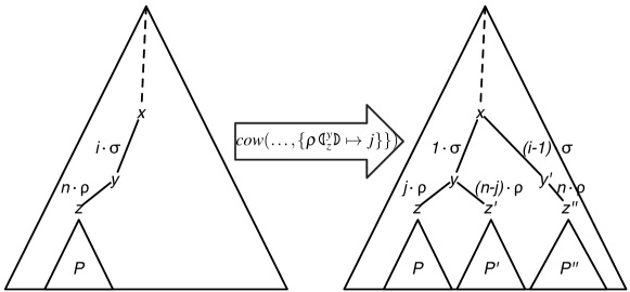
Figure 3: Example copy-on-write of a subterm.

At this point, the reaction is executed, by removing the reactants $S_{1}$ from the machine term (via the operation $\ominus$), adding the products $S_{2}$ (via the operation $\oplus$) and updating the current time of the machine. The function $f$ performs any global “clean-up” and restructuring to the machine term that may be required by the reaction (e.g., garbage collection, elimination of names not used anymore,…). Moreover, since a reaction can rearrange the hierarchy structure, possibly creating new compartments and deleting others, we have to add to the environment any fresh name introduced in the products.

Finally, the term can be “normalized” by collapsing equivalent copies of the same subtree into a single copy (with the right multiplicity), by the function $norm(\_)$. In its simplest form, $norm(\_)$ can be the identity, i.e., no normalization is performed at all. Although this is correct, it can lead to unnecessary copies of the same subtrees. We can define $norm(\_)$ such that

$$norm(\{I_{1}\mapsto i_{1},I_{2}\mapsto i_{2}\}\cup S,R)=norm(\{I_{1}\mapsto i_{1}+i_{2}\}\cup S,R[I_{2}/I_{1}])\quad\text{if }I_{1}\equiv I_{2}$$

where the equivalence between species can be implemented by comparing the subtrees starting from $I_{1}$, $I_{2}$, e.g., by calculating a suitable hash value. We leave this refinement as future development.

In order to implement the Next Reaction method, each reaction $O$ is associated with a pair $R(O)=(a,t)$, where $a$ is the reaction propensity and $t$ is the time at which the reaction is supposed to occur. The function $delay(r,a)$ computes a time interval from a random variable with rate $r$ and propensity $a$.

This general structure can be instantiated with a given process calculus, just by providing the definition for the missing parts. Given a set $Proc$ of processes, we have to define:

1. the syntax of the species $I$ (which may be different from that of processes);

2. a function $species_{E,x}(P)$ mapping a process $P\in Proc$ to a species set located in $x$;

3. a function $reactions(I\mapsto i,S)$ for computing the multiset of reactions between a (new) species I with multiplicity $i$ and a population of (existing) species $S$.

The function $species$ is used to initialise the abstract machine at the beginning of a simulation. If we aim to simulate the execution of a process $P\in Proc$, the corresponding initial state (rooted in $root$) is

$$\llparenthesis P\rrparenthesis_{root}\triangleq fn(J)\vdash J\oplus(0,\emptyset,\emptyset)\quad\text{ where }J=species_{\emptyset,root}(P).$$

The $reactions$ function is used to adjust the set of possible reactions dynamically.

5 Implementing the Stochastic Brane Calculus in COWGSAM

In this section, we show how the COW Generic Stochastic Abstract Machine can be used to implement the Stochastic Brane Calculus, following the protocol described in the previous section.

5.1 Encoding of the Stochastic Brane Calculus

Syntax of species

We define the species for the brane calculus, which in turn lead us to introduce complexes and actions. Notice that (despite the deceiving syntax) species are not systems and complexes are not membranes; nevertheless, actions are a subset of membranes.

$$I::=\ C\bananaleft^{x}_{y}\bananaright$$ (Species)

$$C::=\ A_{1},\ldots,A_{n}$$ (Complexes)

$$A::=\ \nwarrowin_{n}.\sigma\mid\nwarrowin^{\smallbot}_{n}(\tau).\sigma\mid\nwarrowout_{n}.\sigma\mid\nwarrowout^{\smallbot}_{n}.\sigma\mid\ocirc_{n}(\tau).\sigma$$ (Actions)

Node names can appear in the species in $S$ and in reactions $R$.

The $species$ function

We can now provide the definition of the translation of a process $P\in\mathbb{B}_{\mathsf{sys}}$ into a species set. Basically, each compartment is assigned a different, fresh node name; therefore, the function $species_{E,x}(P)$ is parametric in the set $E$ of allocated node names, and the name $x\in E$ to be used as the location of the system $P$. The name $x$ changes as we descend the compartment hierarchy.

In order to capture correctly the multiplicity of each species, we assume that systems are in normal form. Basically, this form is a shorthand for products where $n$ copies of the same system, i.e., $P\circ\dots\circ P$, are represented as $n\cdot P$.

$$\text{Normal Systems}::\mathbb{B}_{\mathsf{sys}}^{n}\qquad Q\mathrel{::=}n_{1}\cdot\sigma_{1}\bananaleft Q_{1}\bananaright\smallcirc\dots\smallcirc n_{k}\cdot\sigma_{k}\bananaleft Q_{k}\bananaright\\ \text{ where }k\geq 0\text{ and for }i\neq j:\sigma_{i}\bananaleft Q_{i}\bananaright\not\equiv\sigma_{j}\bananaleft Q_{j}\bananaright$$

A system in normal form can be translated into a system just by unfolding the products. For $Q\in\mathbb{B}_{\mathsf{sys}}^{n}$ a system in normal form, let $\lceil Q\rceil\in\mathbb{B}_{\mathsf{sys}}$ defined as follows:

$$\lceil\smalldiam\rceil=\smalldiam\qquad\lceil n\cdot\sigma\bananaleft Q^{\prime}\bananaright\circ Q^{\prime\prime}\rceil=\overbrace{\sigma\bananaleft\lceil Q^{\prime}\rceil\bananaright\circ\dots\circ\sigma\bananaleft\lceil Q^{\prime}\rceil\bananaright}^{n\text{ times}}\circ\lceil Q^{\prime\prime}\rceil$$

Proposition 5.1.

For all $P\in\mathbb{B}_{\mathsf{sys}}$, there exists a system in normal form $Q\in\mathbb{B}_{\mathsf{sys}}^{n}$ such that $\lceil Q\rceil\equiv P$.

As a consequence, we can give the definition of $species$ on systems in normal form, as follows:

$$species_{E,x}(\smalldiam)\triangleq\ \emptyset$$

$$species_{E,x}(n\cdot\sigma\bananaleft Q_{1}\bananaright\circ Q_{2})\triangleq\ \{s(\sigma)\bananaleft^{x}_{y}\bananaright\mapsto n\}\cup species_{E\uplus\{y\},y}(Q_{1})\cup species_{E,x}(Q_{2})$$

$$\text{with }\ y\notin E\text{ and }fn(species_{E\uplus\{y\},y}(Q_{1}))\cap fn(species_{E,x}(Q_{2}))\subseteq\{x\}$$

The condition in the second case ensures that two different compartments are never given the same name—any name clash has to be resolved by an $\alpha$-conversion. The function $s(\_)$ converts a membrane into a set of complexes:

$$s(\mathbf{0})\triangleq\ \emptyset \qquad s(\sigma|\sigma^{\prime})\triangleq\ s(\sigma)\cup s(\sigma^{\prime}) \qquad s(\pi.\sigma)\triangleq\ \{\pi.\sigma\}$$

The $reactions$ function

The next step is to define the function $reactions(I\mapsto i,S)$, for $I$ a species with multiplicity $i$ and $S$ a population.

$$reactions_{E}(I_{1}\mapsto i,S)\triangleq\ unary_{E}(I_{1})\cup binary_{E}(I_{1},S)$$

$$unary_{E}(I_{1})\triangleq\ \{(\{I_{1}\mapsto 1\},r_{n},id,\{(s(\sigma)\cup U_{1}^{\prime})\bananaleft^{x}_{y}\bananaright\mapsto 1,s(\rho)\bananaleft^{y}_{w}\bananaright\mapsto 1\})\mid$$

$$\hskip 56.9055ptI_{1}=U_{1}\bananaleft^{x}_{y}\bananaright,~{}U_{1}=\{\ocirc_{n}(\rho).\sigma\}\cup U_{1}^{\prime},w\notin E\}$$

$$binary_{E}(I_{1},S)\triangleq\ \left\{(\{I_{1}\mapsto 1,I_{2}\mapsto 1\},r_{n},f,\{(s(\tau)\cup U^{\prime}_{1}\cup s(\sigma)\cup U^{\prime}_{2})\bananaleft^{x}_{y}\bananaright\mapsto 1\})\mid I_{2}\in dom(S),\right.$$

$$\hskip 56.9055pt(I_{1}=U_{1}\bananaleft^{x}_{y}\bananaright,I_{2}=U_{2}\bananaleft^{y}_{w}\bananaright)\vee(I_{2}=U_{1}\bananaleft^{x}_{y}\bananaright,I_{1}=U_{2}\bananaleft^{y}_{w}\bananaright),$$

$$\hskip 56.9055pt\left.U_{1}=\{\nwarrowout^{\smallbot}_{n}.\tau\}\cup U^{\prime}_{1},U_{2}=\{\nwarrowout_{n}.\sigma\}\cup U^{\prime}_{2},f=\lambda T.T[w:=x]\right\}\ \uplus$$

$$\left\{(\{I_{1}\mapsto 1,I_{2}\mapsto 1\},r_{n},id,\phantom{U^{\prime}_{1}}\right.$$

$$\hskip 28.45274pt\{(s(\tau)\cup U^{\prime}_{1})\bananaleft^{x}_{y}\bananaright\mapsto 1,s(\rho)\bananaleft^{y}_{w}\bananaright\mapsto 1,(s(\sigma)\cup U^{\prime}_{2})\bananaleft^{w}_{z}\bananaright\mapsto 1\})\mid I_{2}\in dom(S),$$

$$\hskip 56.9055pt(I_{1}=U_{1}\bananaleft^{x}_{y}\bananaright,I_{2}=U_{2}\bananaleft^{x}_{z}\bananaright)\vee(I_{2}=U_{1}\bananaleft^{x}_{y}\bananaright,I_{1}=U_{2}\bananaleft^{x}_{z}\bananaright),$$

$$\hskip 56.9055pt\left.U_{1}=\{\nwarrowin^{\smallbot}_{n}(\rho).\tau\}\cup U^{\prime}_{1},U_{2}=\{\nwarrowin_{n}.\sigma\}\cup U^{\prime}_{2},~{}w\notin E\right\}$$

In the case of Brane Calculus, the unary reactions are only those arising from pinocytosis, while binary reactions arise from exocytosis and phagocytosis. In both cases, the multiplicity of each reactant is 1, so the multiplicity of $I_{1}$ is not relevant. Exocytosis merges two compartments; this is reflected by the fact that the “rearranging” function $f$ substitutes every occurrence of the name $w$ in $T$ with $x$. On the other hand, pinocytosis and phagocytosis create new compartments; to represent the new structure, we choose a fresh name $w$ representing the new intermediate nesting level, and reconnect the various compartments accordingly. Therefore, for any reaction $(S_{1},r,f,S_{2})\in reactions_{E}(I_{1}\mapsto i,S)$, $fn(S_{2})\setminus E$ is either $\emptyset$ (in the case of exocytosis) or the singleton $\{w\}$.

5.2 Adequacy results

Before proving the correctness of our implementation, we have to define how to translate a species set back to a system of the brane calculus.

Let $S$ be a non empty species set. A root name of $S$, denoted by $root(S)$, is a name $x$ such that $S(C\bananaleft^{x}_{y}\bananaright)>0$ for some $C,y$, and for all $z,C^{\prime}:C^{\prime}\bananaleft^{z}_{x}\bananaright\notin dom(S)$. The next result states that $root(\_)$ is well defined on the species sets we encounter during a simulation.

Lemma 5.2.

For all $P\in\mathbb{B}_{\mathsf{sys}}$:

1. if $P\neq\smalldiam$: $root(\llparenthesis P\rrparenthesis_{x})=x$.

2. if $\llparenthesis P\rrparenthesis_{x}\xrightarrow{a,O}E\vdash(t,S,R)$ and $S\neq\emptyset$, then $root(S)=x$.

Proof.

(1.) is trivial by definition. (2.) It is enough to check that the reaction rules introduced by $reactions(\_)$ do not change the name of the root, nor introduce new ones. ∎

We can now define a function $\llbracket\_\rrbracket$ which maps complexes to membranes, and a function $\llbracket\_\rrbracket_{x}$ mapping species sets to systems; the latter is parametric in the name $x$ of the root of the system.

$$\llbracket A_{1},\dots,A_{n}\rrbracket\triangleq A_{1}|\dots|A_{n}\qquad\llbracket S\rrbracket_{x}\triangleq\prod_{C\bananaleft^{x}_{y}\bananaright\in dom(S)}{S(C\bananaleft^{x}_{y}\bananaright)}\cdot(\llbracket C\rrbracket\bananaleft\llbracket S\rrbracket_{y}\bananaright)$$

where the notation $n\cdot P$ is a shorthand for $P\smallcirc\dots\smallcirc P$, $n$ times.

Lemma 5.3.

For all $P\in\mathbb{B}_{\mathsf{sys}}$:

1. $\llbracket\llparenthesis P\rrparenthesis_{x}\rrbracket_{x}\equiv P$.

2. if $\llparenthesis P\rrparenthesis_{x}\xrightarrow{a,O}E\vdash(t,S,R)$ then $\llbracket S\rrbracket_{x}$ is well defined.

Proof.

(1.) is easy. (2.) It is enough to check that the reaction rules introduced by $reactions(\_)$ do not introduce loops (i.e., the order among names is well founded). ∎

We can now state and prove the main results of this section.

Proposition 5.4 (Soundness).

For all $P\in\mathbb{B}_{\mathsf{sys}}$, if $\llparenthesis P\rrparenthesis_{x}\xrightarrow{a,O}E\vdash(t,S,R)$ then there exists $\mu$ such that $P\xrightarrow{}\mu$ and $\mu_{id}([\llbracket S\rrbracket_{x}])=a$.

Proof.

The proof is by cases on which reaction rule $O$ is selected by the function $next$. By additivity of measures, we can restrict ourselves to when the whole process $P$ is the redex of the reduction. Let us see here the case when $P$ is the redex of a (red-pino) (another is in Appendix B).

Let $P=\ocirc_{n}(\rho).\sigma|\sigma_{0}\bananaleft P^{\prime}\bananaright$ and let us assume that $\sigma_{0}$ does not exhibit a $\ocirc_{n}$ action. Then, the translation of $P$ is $\llparenthesis P\rrparenthesis_{x}=E\vdash species_{\emptyset,x}(P)\oplus(0,\emptyset,\emptyset)$, where

$$species_{\emptyset,x}(P) =\{s(\ocirc_{n}(\rho).\sigma|\sigma_{0})\bananaleft^{x}_{y}\bananaright\mapsto 1\}\cup species_{\{y\},x}(P^{\prime})$$

$$=\{(s(\ocirc_{n}(\rho).\sigma)\cup s(\sigma_{0}))\bananaleft^{x}_{y}\bananaright\mapsto 1\}\cup species_{\{y\},x}(P^{\prime})$$

$$=\{(\{\ocirc_{n}(\rho).\sigma\}\cup s(\sigma_{0}))\bananaleft^{x}_{y}\bananaright\mapsto 1\}\cup species_{\{y\},x}(P^{\prime})$$

Let $I_{1}=(\{\ocirc_{n}(\rho).\sigma\}\cup s(\sigma_{0}))\bananaleft^{x}_{y}\bananaright$ and $J_{P^{\prime}}=species_{\{y\},x}(P^{\prime})$; then $\llparenthesis P\rrparenthesis_{x}=I_{1}\mapsto 1\oplus J_{P^{\prime}}\oplus(0,\emptyset,\emptyset)=J_{P^{\prime}}\oplus(0,S^{\prime},R^{\prime})$ where

$$S^{\prime} =\{I_{1}\mapsto 1\}$$

$$R^{\prime} =init(L,(0,S^{\prime},\emptyset))=\{O_{L}\mapsto(t_{1},a_{1})\}$$

$$O_{L} =(\{I_{1}\mapsto 1\},r_{n},id,\{(s(\sigma)\cup s(\sigma_{0}))\bananaleft^{x}_{y}\bananaright\mapsto 1,s(\rho)\bananaleft^{y}_{w}\bananaright\mapsto 1\})$$

$$L =reactions(I_{1}\mapsto 1,\emptyset)=unary(I_{1})=\{(\{I_{1}\mapsto 1\},r_{n},id,\{(s(\sigma)\cup s(\sigma_{0}))\bananaleft^{x}_{y}\bananaright\mapsto 1,s(\rho)\bananaleft^{y}_{w}\bananaright\mapsto 1\})\}$$

Now, the reaction $O$ in $\llparenthesis P\rrparenthesis_{x}\xrightarrow{a,O}T$ is $O_{L}$ (otherwise it would involve $P^{\prime}$, not the pino of the whole $P$). This means that $\llparenthesis P\rrparenthesis_{x}\xrightarrow{a,O}T$ is derived by means of an application of the (Reaction rule) as follows, where $S_{1}=\{I_{1}\mapsto 1\}$ and $S_{2}=\{(s(\sigma)\cup s(\sigma_{0}))\bananaleft^{x}_{y}\bananaright\mapsto 1,s(\rho)\bananaleft^{y}_{w}\bananaright\mapsto 1\}$:

$${\displaystyle\frac{((S_{1},r_{n},id,S_{2}),a_{1},t_{1})=next(0,S^{\prime},R^{\prime})\quad(E^{\prime}\vdash(0,S^{\prime\prime},R^{\prime\prime}))=cow(E\vdash(0,S^{\prime},R^{\prime}),S_{1})}{E\vdash\{J_{P^{\prime}}\}\oplus(0,S^{\prime},R^{\prime})\xrightarrow{a_{1},(S_{1},r_{n},id,S_{2})}norm(E\cup fn(S_{2})\vdash(\{J_{P^{\prime}}\}\oplus S_{2}\oplus((t_{1},S^{\prime\prime},R^{\prime\prime})\ominus S_{1})))}}$$

where $S^{\prime\prime}=S^{\prime}$ and $R^{\prime\prime}=R^{\prime}$.

$\{J_{P^{\prime}}\}\oplus S_{2}\oplus((t_{1},S^{\prime\prime},R^{\prime\prime})\ominus S_{1})=$
                           $=J_{P^{\prime}}\oplus\{(s(\sigma)\cup s(\sigma_{0}))\bananaleft^{x}_{y}\bananaright\mapsto 1,s(\rho)\bananaleft^{y}_{w}\bananaright\mapsto 1\}\oplus((t_{1},S^{\prime},R^{\prime})\ominus\{I_{1}\mapsto 1\})$
                           $=J_{P^{\prime}}\oplus\{(s(\sigma)\cup s(\sigma_{0}))\bananaleft^{x}_{y}\bananaright\mapsto 1,s(\rho)\bananaleft^{y}_{w}\bananaright\mapsto 1\}\oplus(t_{1},\{I_{1}\mapsto 0\},\{O_{L}\mapsto(t_{2},a_{2})\})$
                           $=J_{P^{\prime}}\oplus J^{\prime}\oplus(t_{1},\{I_{1}\mapsto 0\},\{O_{L}\mapsto(t_{2},a_{2})\})$

Now let us define $Q$ as $Q=\sigma|\sigma_{0}\bananaleft\rho\bananaleft\smalldiam\bananaright\smallcirc P^{\prime}\bananaright$, then $\llparenthesis Q\rrparenthesis_{x}=species_{\emptyset,x}(Q)\oplus(0,\emptyset,\emptyset)$ where

$$species_{\emptyset,x}(Q) =species_{\emptyset,x}(\sigma|\sigma_{0}\bananaleft\rho\bananaleft\smalldiam\bananaright\smallcirc P^{\prime}\bananaright)$$

$$=\{s(\sigma|\sigma_{0})\bananaleft^{x}_{y}\bananaright\mapsto 1\}\cup species_{\{x\},y}(\rho\bananaleft\smalldiam\bananaright\smallcirc P^{\prime})$$

$$=\{(s(\sigma)\cup s(\sigma_{0}))\bananaleft^{x}_{y}\bananaright\mapsto 1\}\cup species_{\{x\},y}(\rho\bananaleft\smalldiam\bananaright)\cup species_{\{x\},y}(P^{\prime})$$

$$=\{(s(\sigma)\cup s(\sigma_{0}))\bananaleft^{x}_{y}\bananaright\mapsto 1\}\cup\{s(\rho)\bananaleft^{y}_{w}\bananaright\mapsto 1\}\cup\emptyset\cup J_{P^{\prime}}=J^{\prime}\cup J_{P^{\prime}}$$

and hence $Q\equiv\llbracket J_{P^{\prime}}\oplus J^{\prime}\oplus(t_{1},\{I_{1}\mapsto 0\},\{O_{L}\mapsto(t_{2},a_{2})\})\rrbracket_{x}$. It remains to prove that $r_{n}=\mu_{id}([Q])$. Let us notice that the derivation of $P\to\mu$ is actually as follows:

            $\ocirc_{n}(\rho).\sigma\xrightarrow{}[\ocirc_{n}]_{\sigma}^{\rho}$         $\sigma_{0}\xrightarrow{}\mu^{\prime\prime}$ (par)             $\ocirc_{n}(\rho).\sigma|\sigma_{0}\xrightarrow{}[\ocirc_{n}]^{\rho}_{\sigma}{}_{\ocirc_{n}(\rho).\sigma}\kern-2.0pt\varobar_{\sigma_{0}}\mu^{\prime\prime}$        $P^{\prime}\xrightarrow{}\mu^{\prime}$  (loc)                         $\ocirc_{n}(\rho).\sigma|\sigma_{0}\bananaleft P^{\prime}\bananaright\xrightarrow{}\mu$

where $\mu=\mu^{\prime}@^{\ocirc_{n}(\rho).\sigma|\sigma_{0}}_{P^{\prime}}([\ocirc_{n}]^{\rho}_{\sigma}{}_{\ocirc_{n}(\rho).\sigma}\kern-2.0pt\varobar_{\sigma_{0}}\mu^{\prime\prime})$. Then:

$$\mu_{id}([\sigma|\sigma_{0}\bananaleft\rho\bananaleft\smalldiam\bananaright\smallcirc P^{\prime}\bananaright]) =(\mu^{\prime}@^{\ocirc_{n}(\rho).\sigma|\sigma_{0}}_{P^{\prime}}([\ocirc_{n}]^{\rho}_{\sigma}~{}{}_{\ocirc_{n}(\rho).\sigma}\kern-2.0pt\varobar_{\sigma_{0}}\mu^{\prime\prime}))_{id}([\sigma|\sigma_{0}\bananaleft\rho\bananaleft\smalldiam\bananaright\smallcirc P^{\prime}\bananaright])$$

$$=\mu^{\prime}_{id}([\sigma|\sigma_{0}\bananaleft\rho\bananaleft\smalldiam\bananaright\smallcirc P^{\prime}\bananaright])+([\ocirc_{n}]^{\rho}_{\sigma}{}_{\ocirc_{n}(\rho).\sigma}\kern-2.0pt\varobar_{\sigma_{0}}\mu^{\prime\prime})_{\ocirc_{n}}([\sigma|\sigma_{0}]\times[\rho])$$

$$=([\ocirc_{n}]^{\rho}_{\sigma}{}_{\ocirc_{n}(\rho).\sigma}\kern-2.0pt\varobar_{\sigma_{0}}\mu^{\prime\prime})_{\ocirc_{n}}([\sigma|\sigma_{0}]\times[\rho])$$

$$=([\ocirc_{n}]^{\rho}_{\sigma})_{\ocirc_{n}}([\sigma|\sigma_{0}]\times[\rho])+\mu^{\prime\prime}_{\ocirc_{n}}([\sigma|\sigma_{0}]\times[\rho])$$

$$=r_{n}+\mu^{\prime\prime}_{\ocirc_{n}}([\sigma|\sigma_{0}]\times[\rho])=r_{n}$$

where the last equivalence holds because $\mu^{\prime\prime}_{\ocirc_{n}}([\sigma|\sigma_{0}]\times[\rho])=0$ because we assumed that the reaction does not involve $\sigma_{0}$. ∎

Proposition 5.5 (Progress).

For all processes $P,Q$, if $P\blacklongrightarrow Q$ then there exists a reaction $O$ and a term $T$ such that $\llparenthesis P\rrparenthesis_{x}\xrightarrow{a,O}T$ and $Q\equiv\llbracket T\rrbracket_{x}$.

Proof.

By induction on the derivation of $P\blacklongrightarrow Q$. Let us see the case of (red-pin), the others being similar. Let $P=\ocirc(\rho).\sigma|\sigma_{0}\bananaleft P^{\prime}\bananaright$ and $Q=\sigma|\sigma_{0}\bananaleft\rho\bananaleft\smalldiam\bananaright\smallcirc P^{\prime}\bananaright$. Then,

$$\llparenthesis P\rrparenthesis_{x}=species_{\{y\},x}(P^{\prime})\oplus(0,\{(\{\ocirc_{n}(\rho).\sigma\}\cup s(\sigma_{0}))\bananaleft^{x}_{y}\bananaright\mapsto 1\},\{O_{L}\mapsto(t_{1},a_{1})\})$$

where $O_{L}=(\{(\{\ocirc_{n}(\rho).\sigma\}\cup s(\sigma_{0}))\bananaleft^{x}_{y}\bananaright\mapsto 1\},r_{n},id,\{(s(\sigma)\cup s(\sigma_{0}))\bananaleft^{x}_{y}\bananaright\mapsto 1,s(\rho)\bananaleft^{y}_{w}\bananaright\mapsto 1\})$. Then, by the (Reaction rule) we can take $T=species_{\{x\},y}(P^{\prime})\oplus(t_{1},\{(s(\sigma)\cup s(\sigma_{0}))\bananaleft^{x}_{y}\bananaright\mapsto 1,s(\rho)\bananaleft^{y}_{w}\bananaright\mapsto 1\},\emptyset)$. It is easy to check that $Q\equiv\llbracket T\rrbracket_{x}$. ∎

Proposition 5.6 (Completeness).

For all processes $P,Q$, if $P\xrightarrow{}\mu$ and $\mu_{id}([Q])>0$ then for all node name $x$, there exists a reaction $O$ and a term $T$ such that $\llparenthesis P\rrparenthesis_{x}\xrightarrow{a,O}T$, $Q\equiv\llbracket T\rrbracket_{x}$ and $a=\mu_{id}([Q])$.

Proof.

If $P\xrightarrow{}\mu$ and $\mu_{id}([Q])>0$ then $P\blacklongrightarrow Q$ by Prop. 3.4. By Prop. 5.5, we have that for some $a,O,T$, $\llparenthesis P\rrparenthesis_{x}\xrightarrow{a,O}T$ and $Q\equiv\llbracket T\rrbracket_{x}$. But then $a=\mu_{id}([Q])$ by soundness (Prop. 5.4). ∎

5.3 Example

We conclude this section with an example. Let $P=10000\cdot\nwarrowin_{n}.\nwarrowout_{m}\bananaleft\nwarrowin_{k}\bananaleft\bananaright\bananaright\smallcirc 100\cdot((\nwarrowin^{\smallbot}_{n}(\nwarrowout^{\smallbot}_{m})\mid\nwarrowout^{\smallbot})\bananaleft\nwarrowin_{k}\bananaleft\bananaright\bananaright)$. Then, its reductions in the Brane Calculus are as follows:

$$10000\cdot\nwarrowin_{n}.\nwarrowout_{m}\bananaleft\nwarrowin_{k}\bananaleft\bananaright\bananaright\smallcirc 100\cdot((\nwarrowin^{\smallbot}_{n}(\nwarrowout^{\smallbot}_{m})\mid\nwarrowout^{\smallbot})\bananaleft\nwarrowin_{k}\bananaleft\bananaright\bananaright)$$

$$\blacklongrightarrow 9999\cdot\nwarrowin_{n}.\nwarrowout_{m}\bananaleft\nwarrowin_{k}\bananaleft\bananaright\bananaright\smallcirc 99\cdot((\nwarrowin^{\smallbot}_{n}(\nwarrowout^{\smallbot}_{m})\mid\nwarrowout^{\smallbot})\bananaleft\nwarrowin_{k}\bananaleft\bananaright\bananaright)\smallcirc\nwarrowout^{\smallbot}\bananaleft\nwarrowout^{\smallbot}_{m}\bananaleft\nwarrowout_{m}\bananaleft\nwarrowin_{k}\bananaleft\bananaright\bananaright\bananaright\smallcirc\nwarrowin_{k}\bananaleft\bananaright\bananaright$$

$$\blacklongrightarrow 9999\cdot\nwarrowin_{n}.\nwarrowout_{m}\bananaleft\nwarrowin_{k}\bananaleft\bananaright\bananaright\smallcirc 99\cdot((\nwarrowin^{\smallbot}_{n}(\nwarrowout^{\smallbot}_{m})\mid\nwarrowout^{\smallbot})\bananaleft\nwarrowin^{\smallbot}_{k}()\bananaleft\bananaright\bananaright)\smallcirc\nwarrowout^{\smallbot}\bananaleft 2\cdot\nwarrowin_{k}\bananaleft\bananaright\smallcirc\smalldiam\bananaleft\smalldiam\bananaright\bananaright$$

The translation of $P$ is $\llparenthesis P\rrparenthesis_{x}=E\vdash species_{\emptyset,x}(P)\oplus(0,\emptyset,\emptyset)$, where

$$species_{\emptyset,x}(P) =species_{\{x\}}(10000\cdot\nwarrowin_{n}.\nwarrowout_{m}\bananaleft\nwarrowin_{k}\bananaleft\bananaright\bananaright\circ 100\cdot(\nwarrowin^{\smallbot}_{n}(\nwarrowout^{\smallbot}_{m})\mid\nwarrowout^{\smallbot})\bananaleft\nwarrowin_{k}\bananaleft\bananaright\bananaright)$$

$$=\{s(\nwarrowin_{n}.\nwarrowout_{m})\bananaleft^{x}_{y}\bananaright\mapsto 10000\}\cup species_{\{x,y\},y}(\nwarrowin_{k}\bananaleft\bananaright)\cup\{s(\nwarrowin^{\smallbot}_{n}(\nwarrowout^{\smallbot}_{m})\mid\nwarrowout^{\smallbot})\bananaleft^{x}_{z}\bananaright\mapsto 100\}$$

$$\phantom{=}~{}\cup species_{\{x,z\},z}(\nwarrowin_{k}\bananaleft\bananaright)$$

$$=\{\{\nwarrowin_{n}.\nwarrowout_{m}\}\bananaleft^{x}_{y}\bananaright\mapsto 10000,\{\nwarrowin^{\smallbot}_{n}(\nwarrowout^{\smallbot}_{m}),\nwarrowout^{\smallbot}\}\bananaleft^{x}_{z}\bananaright\mapsto 100,\{\nwarrowin_{k}\}\bananaleft^{y}_{w}\bananaright\mapsto 1,$$

$$\phantom{=}~{}\{\nwarrowin_{k}\}\bananaleft^{z}_{v}\bananaright\mapsto 1\}$$

Let $I_{1}=\{\nwarrowin_{n}.\nwarrowout_{m}\}\bananaleft^{x}_{y}\bananaright$, $I_{2}=\{\nwarrowin^{\smallbot}_{n}(\nwarrowout^{\smallbot}_{m}),\nwarrowout^{\smallbot}\}\bananaleft^{x}_{z}\bananaright$, $I_{3}=\{\nwarrowin_{k}\}\bananaleft^{y}_{w}\bananaright$, $I_{4}=\{\nwarrowin_{k}\}\bananaleft^{z}_{v}\bananaright$, $r_{n}=10s^{-1}$, $r_{k}=5s^{-1}$ and $r_{m}=5s^{-1}$; then

$$\llparenthesis P\rrparenthesis_{x} =I_{1}\mapsto 10000\oplus I_{2}\mapsto 100\oplus I_{3}\mapsto 1\oplus I_{4}\mapsto 1\oplus(0,\emptyset,\emptyset)$$

$$=I_{2}\mapsto 100\oplus I_{3}\mapsto 1\oplus I_{4}\mapsto 1\oplus(0,S_{1},R_{1})$$

$$=I_{3}\mapsto 1\oplus I_{4}\mapsto 1\oplus(0,S_{2},R_{2})$$

$$=I_{4}\mapsto 1\oplus(0,S_{3},R_{3})=(0,S_{4},R_{4})$$

where

$$L_{1} =reactions(I_{1}\mapsto 10000,\emptyset)=\emptyset$$

$$S_{1} =S\{I_{1}\mapsto 10000\}$$

$$R_{1} =R\cup init(L_{1},(0,S_{1},\emptyset))=\emptyset$$

$$L_{2} =reactions(I_{2}\mapsto 100,S_{1})$$

$$=(\{I_{2}\mapsto 1,I_{1}\mapsto 1\},10,id,\{\{\nwarrowout^{\smallbot}\}\bananaleft^{x}_{z}\bananaright\mapsto 1,\{\nwarrowout^{\smallbot}_{m})\}\bananaleft^{z}_{w}\bananaright\mapsto 1,\{\nwarrowout_{m}\}\bananaleft^{w}_{y}\bananaright\mapsto 1\})$$

$$S_{2} =S_{1}\{I_{2}\mapsto 100\}=\{I_{1}\mapsto 10000,I_{2}\mapsto 100\}$$

$$R_{2} =R_{1}\cup init(L_{2},(0,S_{2},R_{1}))=\{O_{L_{2}}\mapsto(t_{1},a_{1})\}$$

$$L_{3} =reactions(I_{3}\mapsto 1,S_{2})=\emptyset$$

$$S_{3} =S_{2}\{I_{3}\mapsto 1\}=\{I_{1}\mapsto 10000,I_{2}\mapsto 100,I_{3}\mapsto 1\}$$

$$R_{3} =R_{2}\cup init(L_{3},(0,S_{3},R_{2}))=R_{2}$$

$$L_{4} =reactions(I_{4}\mapsto 1,S_{3})=\emptyset$$

$$S_{4} =S_{3}\{I_{4}\mapsto 1\}=\{I_{1}\mapsto 10000,I_{2}\mapsto 100,I_{3}\mapsto 1,I_{4}\mapsto 1\}$$

$$R_{4} =R_{3}\cup init(L_{4},(0,S_{4},R_{3}))=R_{3}$$

with $\begin{array}[t]{rl}O_{L_{2}}&=(\{I_{2}\mapsto 1,I_{1}\mapsto 1\},10,id,\{\{\nwarrowout^{\smallbot}\}\bananaleft^{x}_{z}\bananaright\mapsto 1,\{\nwarrowout^{\smallbot}_{m}\}\bananaleft^{z}_{w}\bananaright\mapsto 1,\{\nwarrowout_{m}\}\bananaleft^{w}_{y}\bananaright\mapsto 1\})\\ a_{1}&=propensity(O_{L_{2}},S_{2})=10000000\\ t_{1}&=0+delay(10,10000000).\end{array}$
Now, the reaction $O$ in $\llparenthesis P\rrparenthesis_{x}\xrightarrow{a,O}T$ is $O_{L}$. This means that $\llparenthesis P\rrparenthesis_{x}\xrightarrow{a,O}T$ is derived by means of an application of the (Reaction rule) as follows, where $E=x,y,z,w$, $S_{1}=\{I_{2}\mapsto 1,I_{1}\mapsto 1\}$, and $S_{2}=\{\{\nwarrowout^{\smallbot}\}\bananaleft^{x}_{z}\bananaright\mapsto 1,\{\nwarrowout^{\smallbot}_{m}\}\bananaleft^{z}_{w}\bananaright\mapsto 1,\{\nwarrowout_{m}\}\bananaleft^{w}_{y}\bananaright\mapsto 1\}$:

$${\displaystyle\frac{((S_{1},10,id,S_{2}),10,t_{1})=next(0,S_{4},R_{4})\quad(E^{\prime}\vdash(0,S_{5},R_{5}))=cow(E\vdash(0,S_{4},R_{4}),S_{1})}{\begin{array}[]{l}E\vdash(0,S_{4},R_{4})\xrightarrow{10,(S_{1},10,id,S_{2})}norm(E^{\prime}\cup fn(S_{2})\vdash(S_{2}\oplus((t_{1},S_{5},R_{5})\ominus S_{1})))\end{array}}}$$

where

$$S_{5} =\{I_{1}\mapsto 1,\{\nwarrowin_{n}.\nwarrowout_{m}\}\bananaleft^{x}_{y^{\prime}}\bananaright\mapsto 9999,I_{2}\mapsto 1,\{\nwarrowin^{\smallbot}_{n}(\nwarrowout^{\smallbot}_{m}),\nwarrowout^{\smallbot}\}\bananaleft^{x}_{z^{\prime}}\bananaright\mapsto 99,I_{3}\mapsto 1,$$

$$\phantom{\ =\{}I_{4}\mapsto 1,\{\nwarrowin_{k}\}\bananaleft^{y^{\prime}}_{w^{\prime}}\bananaright\mapsto 1,\{\nwarrowin_{k}\}\bananaleft^{z^{\prime}}_{v^{\prime}}\bananaright\mapsto 1\}$$

$$R_{5} =\{O_{L_{2}}\mapsto(t_{1},a_{1}),O_{1}\mapsto(t_{2},a_{2}),O_{2}\mapsto(t_{3},a_{3}),O_{3}\mapsto(t_{4},a_{4})\}$$

with

$$O_{1} =(\{\{\nwarrowin_{n}.\nwarrowout_{m}\}\bananaleft^{x}_{y^{\prime}}\bananaright\mapsto 1,I_{2}\mapsto 1\},10,id,\{\{\nwarrowout^{\smallbot}\}\bananaleft^{x}_{z}\bananaright\mapsto 1,\{\nwarrowout^{\smallbot}_{m}\}\bananaleft^{z}_{w^{\prime\prime}}\bananaright\mapsto 1,\{\nwarrowout_{m}\}\bananaleft^{w^{\prime\prime}}_{y^{\prime}}\bananaright\mapsto 1\})$$

$$O_{2} =(\{\nwarrowin^{\smallbot}_{n}(\nwarrowout^{\smallbot}_{m}),\nwarrowout^{\smallbot}\}\bananaleft^{x}_{z^{\prime}}\bananaright\mapsto 1,I_{1}\mapsto 1\},10,id,\{\{\nwarrowout^{\smallbot}\}\bananaleft^{x}_{z^{\prime}}\bananaright\mapsto 1,\{\nwarrowout^{\smallbot}_{m}\}\bananaleft^{z^{\prime}}_{w^{\prime\prime\prime}}\bananaright\mapsto 1,\{\nwarrowout_{m}\}\bananaleft^{w^{\prime\prime\prime}}_{y}\bananaright\mapsto 1\})$$

$$O_{3} =(\{\{\nwarrowin_{n}.\nwarrowout_{m}\}\bananaleft^{x}_{y^{\prime}}\bananaright\mapsto 1,\{\nwarrowin^{\smallbot}_{n}(\nwarrowout^{\smallbot}_{m}),\nwarrowout^{\smallbot}\}\bananaleft^{x}_{z^{\prime}}\bananaright\mapsto 1\},10,id,\{\{\nwarrowin^{\smallbot}\}\bananaleft^{x}_{z^{\prime}}\bananaright\mapsto 1,\{\nwarrowout^{\smallbot}_{m}\}\bananaleft^{z^{\prime}}_{z^{\prime\prime}}\bananaright\mapsto 1,\{\nwarrowout_{m}\}\bananaleft^{z^{\prime\prime}}_{y^{\prime}}\bananaright\})$$

$$a_{2} =propensity(O_{1},S_{5})=99990$$

$$a_{3} =propensity(O_{2},S_{5})=990$$

$$a_{4} =propensity(O_{3},S_{5})=989901$$

$$t_{2} =0+delay(10,99990)$$

$$t_{3} =0+delay(10,990)$$

$$t_{4} =0+delay(10,989901)$$

We can now compute the multiset of the new machine state:

$$S_{2}\oplus((t_{1},S_{5},R_{5})\ominus S_{1}) =S_{2}\oplus((t_{1},S_{5},R_{5})\ominus\{I_{2}\mapsto 1,I_{1}\mapsto 1\})$$

$$=S_{2}\oplus((t_{1},S_{6},R_{6}\})\ominus\{I_{1}\mapsto 1\})$$

$$=\{\{\nwarrowout^{\smallbot}\}\bananaleft^{x}_{z}\bananaright\mapsto 1,\{\nwarrowout^{\smallbot}_{m}\}\bananaleft^{z}_{w}\bananaright\mapsto 1,\{\nwarrowout_{m}\}\bananaleft^{w}_{y}\bananaright\mapsto 1\}\oplus(t_{1},S_{7},R_{7})$$

$$=(t_{1},S_{8},R_{8})$$

with

$$a^{\prime}_{2} =propensity(O_{1},S_{6})=0 S_{8} =S_{6}\cup\{\{\nwarrowout^{\smallbot}\}\bananaleft^{x}_{z}\bananaright\mapsto 1,\{\nwarrowout^{\smallbot}_{m}\}\bananaleft^{z}_{w}\bananaright\mapsto 1,\{\nwarrowout_{m}\}\bananaleft^{w}_{y}\bananaright\mapsto 1\}$$

$$t^{\prime}_{2} =t_{1}+(a_{2}/a^{\prime}_{2})(t_{2}-t_{1}) R_{6} =\{O_{1}\mapsto(t^{\prime}_{2},a^{\prime}_{2})\}$$

$$a^{\prime}_{3} =propensity(O_{2},S_{7})=0\qquad\quad R_{7} =R_{6}\cup\{O_{2}\mapsto(t^{\prime}_{3},a^{\prime}_{3})\}$$

$$t^{\prime}_{3} =t_{1}+(a_{3}/a_{5})(t_{3}-t_{1}) R_{8} =R_{7}\cup\{\{\{\nwarrowout^{\smallbot}_{m}\}\bananaleft^{z}_{w}\bananaright\mapsto 1,\{\nwarrowout_{m}\}\bananaleft^{w}_{y}\bananaright\mapsto 1\},5,f,\{\emptyset\bananaleft^{z}_{w}\bananaright\}\mapsto 1\}$$

$$S_{6} =S_{5}\backslash\{I_{2}\mapsto 1\}$$

$$S_{7} =S_{6}\backslash\{I_{1}\mapsto 1\} f =\lambda T.T[y:=z]$$

6 Conclusions

In this paper, we have presented an abstract machine for the Stochastic Brane Calculus. Instead of defining an ad hoc machine, we have adopted the generic abstract machine for stochastic calculi (GSAM) recently introduced by Lakin, Paulevé and Phillips. According to the encoding technique we have adopted, membranes are flattened into a set of species, where the hierarchical structure is represented by means of names. In order to keep track of these names, and for dealing efficiently with multiple copies of the same species, we have introduced a new generic abstract machine, called COWGSAM, which extends the GSAM with a name environment and a copy-on-write optimization strategy. We have proved that the implementation of the Stochastic Brane Calculus in COWGSAM is adequate with respect to the stochastic structural operational semantics of the calculus given in [3].

We think that COWGSAM can be used for implementing other stochastic calculi dealing with nested structures, also beyond the models for systems biology. In particular, it is interesting to apply this approach to Stochastic Bigraphs [10], a general meta-model well-suited for representing a range of stochastic systems with compartments; in this way we would obtain a General Stochastic Bigraphical Machine, which could be instantiated to any given stochastic bigraphic reactive system. However, such a machine would not scale well, as in general the COW strategy may be not very useful; thus, we can restrict our attentions to smaller subsets of BRSs, specifically designed to some application domain. For biological applications, the bigraphic reactive systems considered in [2, 8] might be a more reasonable target.

Another interesting question is about the expressive power of GSAM and COWGSAM. We think that GSAM correspond to stochastic (multiset) Petri nets, but COWGSAM could go further thanks to the possibility of creating unlimited new names during execution. Further work include comparison with other stochastic simulation tools dealing with compartments, like BioPEPA [7].

Acknowledgment Work funded by MIUR PRIN project “SisteR”, prot. 20088HXMYN.

Appendix A Some measure theory

Given a set $M$, a family $\Sigma$ of subsets of $M$ is called a $\sigma$-algebra if it contains $M$ and is closed under complements and (infinite) countable unions:

1. $M\in\Sigma$;

2. $A\in\Sigma$ implies $A^{c}\in\Sigma$, where $A^{c}=M\setminus A$;

3. $\{A_{i}\}_{i\in\mathbb{N}}\subset\Sigma$ implies $\bigcup_{i\in\mathbb{N}}A_{i}\in\Sigma$.

Since $M\in\Sigma$ and $M^{c}=\emptyset$, $\emptyset\in\Sigma$, hence $\Sigma$ is nonempty by definition. A $\sigma$-algebra is closed under countable set-theoretic operations: is closed under finite unions ($A,B\in\Sigma$ implies $A\cup B=A\cup B\cup\emptyset\cup\emptyset\cup\dots\in\Sigma$), countable intersections (by DeMorgan’s law $A\cap B=(A^{c}\cup B^{c})^{c}$ in its finite and inifite version), and countable subtractions ($A,B\in\Sigma$ implies $A\setminus B=A\cap B^{c}\in\Sigma$).

Definition A.1 (Measurable Space).

Given a set $M$ and a $\sigma$-algebra on $M$, the tuple $(M,\Sigma)$ is called a measurable space, the elements of $\Sigma$ measurable sets, and $M$ the support-set.

A set $\Omega\subseteq 2^{M}$ is a generator for the $\sigma$-algebra $\Sigma$ on $M$ if $\Sigma$ is the closure of $\Omega$ under complement and countable union; we write $\sigma(\Omega)=\Sigma$ and say that $\Sigma$ is generated by $\Omega$. Note that the $\sigma$-algebra generated by a $\Omega$ is also the smallest $\sigma$-algebra containing $\Omega$, that is, the intersection of all $\sigma$-algebras that contain $\Omega$. In particular it holds that a completely arbitrary intersection of $\sigma$-algebras is a $\sigma$-algebra. A $\sigma$-algebra generated by $\Omega$, denoted by $\sigma(\Omega)$, is minimal in the sense that if $\Omega\subset\Sigma$ and $\Sigma$ is a $\sigma$-algebra, then $\sigma(\Omega)\subset\Sigma$. If $\Omega$ is a $\sigma$-algebra then obviously $\sigma(\Omega)=\Omega$; if $\Omega$ is empty or $\Omega=\{\emptyset\}$, or $\Omega=\{M\}$, then $\sigma(\Omega)=\{\emptyset,M\}$; if $\Omega\subset\Sigma$ and $\Sigma$ is a $\sigma$-algebra, then $\sigma(\Omega)\subset\Sigma$. A generator $\Omega$ for $\Sigma$ is a base for $\Sigma$ if it has disjoin elements. Note that if $\Omega$ is a base for $\Sigma$, all measurable sets in $\Sigma$ can be decomposed into countable unions of elements in $\Omega$.

A measure on a measurable space $(M,\Sigma)$ is a function $\mu\colon\Sigma\to\mathbb{R}^{+}_{\infty}$, where $\mathbb{R}^{+}_{\infty}$ denotes the extended positive real line, such that

1. $\mu(\emptyset)=0$;

2. for any disjoint sequence $\{N_{i}\}_{i\in I}\subseteq\Sigma$ with $I\subseteq\mathbb{N}$, it holds

   $$\textstyle\mu(\bigcup_{i\in I}N_{i})=\sum_{i\in I}\mu(N_{i})\,.$$

The triple $(M,\Sigma,\mu)$ is called a measure space. A measure space $(M,\Sigma,\mu)$ is called finite if $\mu(M)$ is a finite real number; it is called $\sigma$-finite if $M$ can be decomposed into a countable union of measurable sets of finite measure, that is, $M=\bigcup_{i\in I}N_{i}$, for some $I\subseteq\mathbb{N}$ and $\mu(N_{i})\in\mathbb{R}^{+}$ for each $i\in I$. A set in a measure space has $\sigma$-finite measure if it is a countable union of sets with finite measure. Specifying a measure includes specifying its domain. If $\mu$ is a measure on a measurable space $(M,\Sigma)$ and $\Sigma^{\prime}$ is a $\sigma$-algebra contained in $\Sigma$, then the restriction $\mu^{\prime}$ of $\mu$ to $\Sigma^{\prime}$ is also a measure, and in particular a measure on $(M^{\prime},\Sigma^{\prime})$, for some $M^{\prime}\subseteq M$ such that $\Sigma^{\prime}$ is a $\sigma$-algebra on $M^{\prime}$.

Given two measurable spaces and measures on them, one can obtain the product measurable space and the product measure on that space. Let $(M_{1},\Sigma_{1})$ and $(M_{2},\Sigma_{2})$ be measurable spaces, and $\mu_{1}$ and $\mu_{2}$ be measures on these spaces. Denote by $\Sigma_{1}\otimes\Sigma_{2}$ the $\sigma$-algebra on the cartesian product $M_{1}\times M_{2}$ generated by subsets of the form $B_{1}\times B_{2}$, said rectangles, where $B_{1}\in\Sigma_{1}$ and $B_{2}\in\Sigma_{2}$. The product measure $\mu_{1}\otimes\mu_{2}$ is defined to be the unique measure on the measurable space $(M_{1}\times M_{2},\Sigma_{1}\otimes\Sigma_{2})$ such that, for all $B_{1}\in\Sigma_{1}$ and $B_{2}\in\Sigma_{2}$

$$(\mu_{1}\otimes\mu_{2})(B_{1}\times B_{2})=\mu_{1}(B_{1})\cdot\mu_{2}(B_{2})$$

The existence of this measure is guaranteed by the Hahn-Kolmogorov theorem. The uniqueness of the product measure is guaranteed only in the case that both $(M_{1},\Sigma_{1},\mu_{1})$ and $(M_{2},\Sigma_{2},\mu_{2})$ are $\sigma$-finite.

Let $\Delta(M,\Sigma)$ be the family of measures on $(M,\Sigma)$. It can be organized as a measurable space by considering the $\sigma$-algebra generated by the sets $\{\mu\in\Delta(M,\Sigma):\mu(S)\geq r\}$, for arbitrary $S\in\Sigma$ and $r>0$.

Given two measurable spaces $(M,\Sigma)$ and $(N,\Theta)$ a mapping $f\colon M\to N$ is measurable if for any $T\in\Theta$, $f^{-1}(T)\in\Sigma$. Measurable functions are closed under composition: given $f\colon M\to N$ and $g\colon N\to O$ measurable functions then $g\circ f\colon M\to O$ is also measurable.

Appendix B Proof of Prop. 5.4

Let $P=\nwarrowout^{\smallbot}_{n}.\tau|\tau_{0}\bananaleft\nwarrowout_{n}.\sigma|\sigma_{0}\bananaleft P^{\prime}\bananaright\smallcirc P^{\prime\prime}\bananaright$; then, $\llparenthesis P\rrparenthesis_{x}=E\vdash species_{\emptyset,x}(P)\oplus(0,\emptyset,\emptyset)$, where

$$species_{\emptyset,x}(P)=\{s(\nwarrowout^{\smallbot}_{n}.\tau|\tau_{0})\bananaleft^{x}_{y}\bananaright\}\cup species_{\{x\},y}(\nwarrowout_{n}.\sigma|\sigma_{0}\bananaleft P^{\prime}\bananaright\smallcirc P^{\prime\prime})$$

$$=\{(\{\nwarrowout^{\smallbot}_{n}.\tau\}\cup s(\tau_{0}))\bananaleft^{x}_{y}\bananaright\mapsto 1\}\cup species_{\{x\},y}(\nwarrowout_{n}.\sigma|\sigma_{0}\bananaleft P^{\prime}\bananaright)\cup species_{\{x\},y}(P^{\prime\prime})$$

$$=\{(\{\nwarrowout^{\smallbot}_{n}.\tau\}\cup s(\tau_{0}))\bananaleft^{x}_{y}\bananaright\mapsto 1\}\cup\{s(\nwarrowout_{n}.\sigma|\sigma_{0})\bananaleft^{y}_{w}\bananaright\mapsto 1\}\cup species_{\{x,y\},w}(P^{\prime})\cup species_{\{x\},y}(P^{\prime\prime})$$

$$=\{(\{\nwarrowout^{\smallbot}_{n}.\tau\}\cup s(\tau_{0}))\bananaleft^{x}_{y}\bananaright\mapsto 1\}\cup\{(s(\nwarrowout_{n}.\sigma)\cup s(\sigma_{0}))\bananaleft^{y}_{w}\bananaright\mapsto 1\}\cup species_{\{x,y\},w}(P^{\prime})\cup species_{\{x\},y}(P^{\prime\prime})$$

$$=\{(\{\nwarrowout^{\smallbot}_{n}.\tau\}\cup s(\tau_{0}))\bananaleft^{x}_{y}\bananaright\mapsto 1\}\cup\{(\{\nwarrowout_{n}.\sigma\}\cup s(\sigma_{0}))\bananaleft^{y}_{w}\bananaright\mapsto 1\}\cup species_{\{x,y\},w}(P^{\prime})\cup species_{\{x\},y}(P^{\prime\prime})$$

Let $I_{1}=(\{\nwarrowout^{\smallbot}_{n}.\tau\}\cup s(\tau_{0}))\bananaleft^{x}_{y}\bananaright$, $I_{2}=(\{\nwarrowout_{n}.\sigma\}\cup s(\sigma_{0}))\bananaleft^{y}_{w}\bananaright$, $J_{P^{\prime}}=species_{\{x,y\},w}(P^{\prime})$, $J_{P^{\prime\prime}}=species_{\{x\},y}(P^{\prime\prime})$; then $\llparenthesis P\rrparenthesis_{x}=I_{1}\mapsto 1\oplus I_{2}\mapsto 1\oplus J_{P^{\prime}}\oplus J_{P^{\prime\prime}}\oplus(0,\emptyset,\emptyset)=I_{2}\mapsto 1\oplus J_{P^{\prime}}\oplus J_{P^{\prime\prime}}\oplus(0,S^{\prime},R^{\prime})=J_{P^{\prime}}\oplus J_{P^{\prime\prime}}\oplus(0,S^{\prime\prime},R^{\prime\prime})$ where

$$L^{\prime} =reactions(I_{1}\mapsto 1,\emptyset)=\emptyset$$

$$S^{\prime} =S\{I_{1}\mapsto 1\}$$

$$R^{\prime} =init(L^{\prime},(0,S^{\prime},\emptyset))=\emptyset$$

$$L^{\prime\prime} =reactions(I_{2}\mapsto 1,S^{\prime})$$

$$=(\{I_{2}\mapsto 1,I_{1}\mapsto 1\},r_{n},f,\{(s(\tau)\cup s(\tau_{0})\cup s(\sigma)\cup s(\sigma_{0}))\bananaleft^{x}_{y}\bananaright\mapsto 1\})$$

$$S^{\prime\prime} =S^{\prime}\{I_{2}\mapsto 1\}=\{I_{1}\mapsto 1,I_{2}\mapsto 1\}$$

$$R^{\prime\prime} =init(L^{\prime\prime},(0,S^{\prime\prime},R^{\prime}))=\{O_{L}\mapsto(t_{1},a_{1})\}$$

with $O_{L}=(\{I_{1}\mapsto 1,I_{2}\mapsto 1\},r_{n},f,\{(s(\tau)\cup s(\tau_{0})\cup s(\sigma)\cup s(\sigma_{0}))\bananaleft^{x}_{y}\bananaright\mapsto 1\})$. Now, the reaction $O$ in $\llparenthesis P\rrparenthesis_{x}\xrightarrow{F,O}T$ is $O_{L}$. This means that $\llparenthesis P\rrparenthesis_{x}\xrightarrow{F,O}T$ is derived by means of an application of the (Reaction rule) as follows, where $S_{1}=\{I_{1}\mapsto 1,I_{2}\mapsto 1\}$, $S_{2}=\{(s(\tau)\cup s(\tau_{0})\cup s(\sigma)\cup s(\sigma_{0}))\bananaleft^{x}_{y}\bananaright\mapsto 1\}$ and $f=T[w:=x]$:

$${\displaystyle\frac{((S_{1},r_{n},f,S_{2}),a_{1},t_{1})=next(0,S^{\prime\prime},R^{\prime\prime})\quad(E^{\prime}\vdash(0,S^{\prime\prime\prime},R^{\prime\prime\prime}))=cow(E\vdash(0,S^{\prime\prime},R^{\prime\prime}),S_{1})}{\begin{array}[]{l}E\vdash(0,S^{\prime\prime},R^{\prime\prime})\xrightarrow{a_{1},(S_{1},r_{n},f,S_{2})}norm(E^{\prime}\cup fn(S_{2})\vdash(f(S_{2}\oplus((t_{1},S^{\prime\prime\prime},R^{\prime\prime\prime})\ominus S_{1}))))\end{array}}}$$

where $S^{\prime\prime\prime}=S^{\prime\prime}$ and $R^{\prime\prime\prime}=R^{\prime\prime}$.

$$(f(S_{2}\oplus((t_{1},S^{\prime\prime\prime},R^{\prime\prime\prime})\ominus S_{1}))))=$$

$$=f((s(\tau)\cup s(\tau_{0})\cup s(\sigma)\cup s(\sigma_{0})\bananaleft^{x}_{y}\bananaright)\oplus((t_{1},S^{\prime\prime\prime},R^{\prime\prime\prime})\ominus\{I_{1}\mapsto 1,I_{2}\mapsto 1\})$$

$$=f((s(\tau)\cup s(\tau_{0})\cup s(\sigma)\cup s(\sigma_{0})\bananaleft^{x}_{y}\bananaright)\oplus((t_{1},\{I_{1}\mapsto 0,I_{2}\mapsto 1\},\{O_{L}\mapsto(t_{2},a_{2})\})\ominus\{I_{2}\mapsto 1\})$$

$$=f((s(\tau)\cup s(\tau_{0})\cup s(\sigma)\cup s(\sigma_{0})\bananaleft^{x}_{y}\bananaright)\oplus(t_{1},\{I_{1}\mapsto 0,I_{2}\mapsto 0\},\{O_{L}\mapsto(t_{3},a_{3})\})$$

$$=(s(\tau)\cup s(\tau_{0})\cup s(\sigma)\cup s(\sigma_{0})\bananaleft^{x}_{y}\bananaright)\oplus(t_{1},\{I_{1}\mapsto 0,I_{2}\mapsto 0\},\{O_{L}\mapsto(t_{3},a_{3})\})$$

$$=J^{\prime}\oplus(t_{1},\{I_{1}\mapsto 0,I_{2}\mapsto 0\},\{O_{L}\mapsto(t_{3},a_{3})\})$$

Now let us define $Q$ as $Q=\sigma|\sigma_{0}|\tau|\tau_{0}\bananaleft P^{\prime\prime}\bananaright\smallcirc P^{\prime}$, then $\llparenthesis Q\rrparenthesis_{x}=species_{\emptyset,x}(Q)\oplus(0,\emptyset,\emptyset)$ where

$$species_{\emptyset,x}(Q) =species_{\emptyset,x}(\sigma|\sigma_{0}|\tau|\tau_{0}\bananaleft P^{\prime\prime}\bananaright\smallcirc P^{\prime})$$

$$=species_{\emptyset,x}(\sigma|\sigma_{0}|\tau|\tau_{0}\bananaleft P^{\prime\prime}\bananaright)\cup species_{\emptyset,x}(P^{\prime})$$

$$=\{s(\sigma|\sigma_{0}|\tau|\tau_{0})\bananaleft^{x}_{y}\bananaright)\mapsto 1\}\cup species_{\{x\},y}(P^{\prime\prime})\cup species_{\emptyset,x}(P^{\prime})$$

$$=\{s(\tau)\cup s(\tau_{0})\cup s(\sigma)\cup s(\sigma_{0})\bananaleft^{x}_{y}\bananaright\mapsto 1\}\cup J_{P^{\prime\prime}}\cup J_{P^{\prime}}=J^{\prime}\cup J_{P^{\prime\prime}}\cup J_{P^{\prime}}$$

And hence $Q\equiv\llbracket J_{P^{\prime}}\oplus J_{P^{\prime\prime}}\oplus J^{\prime}\oplus(t_{1},\{I_{1}\mapsto 0,I_{2}\mapsto 0\},\{O_{L}\mapsto(t_{3},a_{3})\})\rrbracket_{x}$. It remains to prove that $r_{n}=\mu_{id}([Q])$. Let us notice that the derivation of $P\xrightarrow{}\mu$ is actually as follows:

       $\nwarrowout^{\smallbot}_{n}.\tau\xrightarrow{}[\nwarrowout^{\smallbot}_{n}]_{\tau}$         $\tau_{0}\xrightarrow{}\mu$ ​​​​​(par)           $\nwarrowout^{\smallbot}_{n}.\tau|\tau_{0}\xrightarrow{}[\nwarrowout^{\smallbot}_{n}]_{\tau}{}_{\nwarrowout^{\smallbot}_{n}.\tau}\kern-2.0pt\varobar_{\tau_{0}}\mu$               $\nwarrowout_{n}.\sigma\xrightarrow{}[\nwarrowout_{n}]_{\sigma}$         $\sigma_{0}\xrightarrow{}\mu^{\prime\prime}$    (par)   $\nwarrowout_{n}.\sigma|\sigma_{0}\xrightarrow{}[\nwarrowout_{n}]_{\sigma}{}_{\nwarrowout_{n}.\sigma}\kern-2.0pt\varobar_{\sigma_{0}}\mu^{\prime\prime}$        $P^{\prime}\xrightarrow{}\mu^{\prime}$    (loc)      $\nwarrowout.\sigma|\sigma_{0}\bananaleft P^{\prime}\bananaright\xrightarrow{}\mu^{\prime}@^{\nwarrowout_{n}.\sigma|\sigma_{0}}_{P^{\prime}}([\nwarrowout_{n}]_{\sigma}{}_{\nwarrowout_{n}.\sigma}\kern-2.0pt\varobar_{\sigma_{0}}\mu^{\prime\prime})$        $P^{\prime\prime}\xrightarrow{}\mu^{\prime\prime\prime}$ ​​​​​​​(comp)            ​​​​​​​$\nwarrowout_{n}.\sigma|\sigma_{0}\bananaleft P^{\prime}\bananaright\smallcirc P^{\prime\prime}\xrightarrow{}(\mu^{\prime}@^{\nwarrowout_{n}.\sigma|\sigma_{0}}_{P^{\prime}}([\nwarrowout_{n}]_{\sigma}{}_{\nwarrowout_{n}.\sigma}\kern-2.0pt\varobar_{\sigma_{0}}\mu^{\prime\prime})){}_{\nwarrowout_{n}.\sigma|\sigma_{0}\bananaleft P^{\prime}\bananaright}\kern-1.0pt\otimes_{P^{\prime\prime}}\mu^{\prime\prime\prime}$  ​​​​​(loc)                                          $\nwarrowout^{\smallbot}_{n}.\tau|\tau_{0}\bananaleft\nwarrowout_{n}.\sigma|\sigma_{0}\bananaleft P^{\prime}\bananaright\smallcirc P^{\prime\prime}\bananaright\xrightarrow{}\nu$

where $\nu=((\mu^{\prime}@^{\nwarrowout_{n}.\sigma|\sigma_{0}}_{P^{\prime}}([\nwarrowout_{n}]_{\sigma}{}_{\nwarrowout_{n}.\sigma}\kern-2.0pt\varobar_{\sigma_{0}}\mu^{\prime\prime})){}_{\nwarrowout_{n}.\sigma|\sigma_{0}\bananaleft P^{\prime}\bananaright}\kern-1.0pt\otimes_{S}\mu^{\prime\prime\prime})@^{\nwarrowout^{\smallbot}_{n}.\tau|\tau_{0}}_{\nwarrowout_{n}.\sigma|\sigma_{0}\bananaleft P^{\prime}\bananaright\smallcirc P^{\prime\prime}}([\nwarrowout^{\smallbot}_{n}]_{\tau}{}_{\nwarrowout^{\smallbot}_{n}.\tau}\kern-2.0pt\varobar_{\tau_{0}}\mu)$,
$\mu_{1}=(\mu^{\prime}@^{\nwarrowout_{n}.\sigma|\sigma_{0}}_{P^{\prime}}([\nwarrowout_{n}]_{\sigma}{}_{\nwarrowout_{n}.\sigma}\kern-2.0pt\varobar_{\sigma_{0}}\mu^{\prime\prime})){}_{\nwarrowout_{n}.\sigma|\sigma_{0}\bananaleft P^{\prime}\bananaright}\kern-1.0pt\otimes_{P^{\prime\prime}}\mu^{\prime\prime\prime}$ and $\mu_{2}=[\nwarrowout^{\smallbot}_{n}]_{\tau}{}_{\nwarrowout^{\smallbot}_{n}.\tau}\kern-2.0pt\varobar_{\tau_{0}}\mu$. Then:

$$\nu_{id}([\sigma|\sigma_{0}|\tau|\tau_{0}\bananaleft P^{\prime\prime}\bananaright\smallcirc P^{\prime}])=(\mu_{1}~{}@^{\nwarrowout^{\smallbot}_{n}.\tau|\tau_{0}}_{\nwarrowout_{n}.\sigma|\sigma_{0}\bananaleft P^{\prime}\bananaright\smallcirc P^{\prime\prime}}~{}\mu_{2})_{id}([\sigma|\sigma_{0}|\tau|\tau_{0}\bananaleft P^{\prime\prime}\bananaright\smallcirc P^{\prime}])$$

$$={\mu_{1}}_{id}([\sigma|\sigma_{0}|\tau|\tau_{0}\bananaleft P^{\prime\prime}\bananaright\smallcirc P^{\prime}])+{\mu_{1}}_{ex_{n}}([\sigma|\sigma_{0}]\times[P^{\prime}]\times[P^{\prime\prime}])\cdot{\mu_{2}}_{\nwarrowout^{\smallbot}_{n}}([\tau|\tau_{0}])/r_{n}$$

$$={\mu_{1}}_{ex_{n}}([\sigma|\sigma_{0}]\times[P^{\prime}]\times[P^{\prime\prime}])\cdot{\mu_{2}}_{\nwarrowout^{\smallbot}_{n}}([\tau|\tau_{0}])/r_{n}$$

$$=({(\mu^{\prime}@^{\nwarrowout_{n}.\sigma|\sigma_{0}}_{P^{\prime}}([\nwarrowout_{n}]_{\sigma}{}_{\nwarrowout_{n}.\sigma}\kern-2.0pt\varobar_{\sigma_{0}}\mu^{\prime\prime}))}_{ex_{n}}([\sigma|\sigma_{0}]\times[P^{\prime}]\times[P^{\prime\prime}])+{\mu^{\prime\prime\prime}_{ex_{n}}([\sigma|\sigma_{0}]\times[P^{\prime}]\times[P^{\prime\prime}])})\cdot{\mu_{2}}_{\nwarrowout^{\smallbot}_{n}}([\tau|\tau_{0}])/r_{n}$$

$$=(([\nwarrowout_{n}]_{\sigma}~{}{}_{\nwarrowout_{n}.\sigma}\kern-2.0pt\varobar_{\sigma_{0}}~{}\mu^{\prime\prime})_{\nwarrowout_{n}}([\sigma|\sigma_{0}])+{\mu^{\prime\prime\prime}_{ex_{n}}([\sigma|\sigma_{0}]\times[P^{\prime}]\times[P^{\prime\prime}])})\cdot{([\nwarrowout^{\smallbot}_{n}]_{\tau}{}_{\nwarrowout^{\smallbot}_{n}.\tau}\kern-2.0pt\varobar_{\tau_{0}}\mu)}_{\nwarrowout^{\smallbot}_{n}}([\tau|\tau_{0}])/r_{n}$$

$$=(([\nwarrowout_{n}]_{\sigma})_{\nwarrowout_{n}}([\sigma|\sigma_{0}])+\mu^{\prime\prime}_{\nwarrowout_{n}}([\sigma|\sigma_{0}])+{\mu^{\prime\prime\prime}_{ex_{n}}([\sigma|\sigma_{0}]\times[P^{\prime}]\times[P^{\prime\prime}])})\cdot(([\nwarrowout^{\smallbot}_{n}]_{\tau})_{\nwarrowout^{\smallbot}_{n}}([\tau|\tau_{0}])+\mu_{\nwarrowout^{\smallbot}_{n}}([\tau|\tau_{0}]))/r_{n}$$

$$=(r_{n}+\mu^{\prime\prime}_{\nwarrowout_{n}}([\sigma|\sigma_{0}])+{\mu^{\prime\prime\prime}_{ex_{n}}([\sigma|\sigma_{0}]\times[P^{\prime}]\times[P^{\prime\prime}])})\cdot(r_{n}+\mu_{\nwarrowout^{\smallbot}_{n}}([\tau|\tau_{0}]))/r_{n}=r_{n}$$

where the last equivalence holds because $\mu^{\prime\prime}_{\nwarrowout_{n}}([\sigma|\sigma_{0}])=\mu^{\prime\prime\prime}_{ex_{n}}([\sigma|\sigma_{0}]\times[P^{\prime}]\times[P^{\prime\prime}])=\mu_{\nwarrowout^{\smallbot}_{n}}([\tau|\tau_{0}])=0$ because we assumed that the reaction does not involve either $\sigma_{0}$ nor $\tau_{0}$.

References

- [1]
- [2] Giorgio Bacci, Davide Grohmann & Marino Miculan (2009): Bigraphical models for protein and membrane interactions. In: Gabriel Ciobanu, editor: Proc. MeCBIC’09, EPTCS 11, pp. 3–18. doi:10.4204/EPTCS.11.1.
- [3] Giorgio Bacci & Marino Miculan (2012): Measurable Stochastics for Brane Calculus. Theoretical Computer Science 431, pp. 117–136. doi:10.1016/j.tcs.2011.12.055.
- [4] Roberto Barbuti, Andrea Maggiolo-Schettini, Paolo Milazzo & Angelo Troina (2007): The Calculus of Looping Sequences for Modeling Biological Membranes. In: George Eleftherakis, Petros Kefalas, Gheorghe Paun, Grzegorz Rozenberg & Arto Salomaa, editors: Workshop on Membrane Computing, Lecture Notes in Computer Science 4860, Springer, pp. 54–76. doi:10.1007/978-3-540-77312-2_4.
- [5] Luca Cardelli (2004): Brane Calculi. In: Vincent Danos & Vincent Schächter, editors: Proc. CMSB, Lecture Notes in Computer Science 3082, Springer, pp. 257–278. doi:10.1007/978-3-540-25974-9_24.
- [6] Luca Cardelli & Radu Mardare (2010): The Measurable Space of Stochastic Processes. In: Proc. QEST, IEEE Computer Society, pp. 171–180. doi:10.1109/QEST.2010.30.
- [7] Federica Ciocchetta & Maria Luisa Guerriero (2009): Modelling Biological Compartments in Bio-PEPA. Electronic Notes in Theoretical Computer Science 227, pp. 77–95. doi:10.1016/j.entcs.2008.12.105.
- [8] Troels Christoffer Damgaard, Espen Højsgaard & Jean Krivine (2012): Formal Cellular Machinery. Electronic Notes in Theoretical Computer Science 284, pp. 55–74. doi:10.1016/j.entcs.2012.05.015.
- [9] Holger Hermanns (2002): Interactive Markov Chains: The Quest for Quantified Quality, Lecture Notes in Computer Science 2428. Springer. doi:10.1007/3-540-45804-2.
- [10] Jean Krivine, Robin Milner & Angelo Troina (2008): Stochastic Bigraphs. In: Proc. 24th MFPS, ENTCS 218, pp. 73–96. doi:10.1016/j.entcs.2008.10.006.
- [11] Matthew R. Lakin, Loïc Paulevé & Andrew Phillips (2012): Stochastic Simulation of Multiple Process Calculi for Biology. Theoretical Computer Science 431, pp. 181–206. doi:10.1016/j.tcs.2011.12.057.
- [12] Cosimo Laneve & Fabien Tarissan (2008): A simple calculus for proteins and cells. Theoretical Computer Science 404(1-2), pp. 127–141. doi:10.1016/j.tcs.2008.04.011.
- [13] Prakash Panangaden (2009): Labelled Markov Processes. Imperial College Press, London, U.K.
- [14] Loïc Paulevé, Simon Youssef, Matthew R. Lakin & Andrew Phillips (2010): A generic abstract machine for stochastic process calculi. In: Paola Quaglia, editor: Proc. CMSB, ACM, pp. 43–54. doi:10.1145/1839764.1839771.
- [15] Aviv Regev, Ekaterina M. Panina, William Silverman, Luca Cardelli & Ehud Y. Shapiro (2004): BioAmbients: an abstraction for biological compartments. Theoretical Computer Science 325(1), pp. 141–167. doi:10.1016/j.tcs.2004.03.061.