Study of the Kinematics and Plasma Properties of A Solar Surge Triggered due to Chromospheric Activity in AR11271

Abstract

We observe a solar surge in NOAA AR11271 using SDO AIA 304 Å image data on 25 August, 2011. The surge rises vertically from its origin upto a height of $\approx$65 Mm with a terminal velocity of $\approx$100 km s^-1, and thereafter falls and fades gradually. The total life time of the surge was $\approx$20 min. We also measure the temperature and density distribution of the observed surge during its maximum rise, and found an average temperature and density of $2.0$ MK and $4.1\times$10⁹ cm^-3, respectively. The temperature map shows the expansion and mixing of cool plasma lagging behind the hot coronal plasma along the surge. As SDO/HMI temporal image data does not show any detectable evidence of the significant photospheric magnetic field cancellation for the formation of the observed surge, we infer that it is probably driven by magnetic reconnection generated thermal energy in the lower chromosphere. The radiance (thus mass density) oscillations near the base of the surge are also evident, which may be the most likely signature of its formation by a reconnection generated pulse. In support of the present observational base-line of the triggering of the surge due to chromospheric heating, we devise a numerical model with conceivable implementation of VAL-C atmosphere and a thermal pulse as an initial trigger. We find that the pulse steepens into a slow shock at higher altitudes that triggers plasma perturbations exhibiting the observed features of the surge, e.g., terminal velocity, height, width, life-time, and heated fine structures near its base.

1 Introduction

Various types of plasma ejections are significant in the solar atmosphere to transport mass and energy at diverse spatio-temporal scales (e.g., Bohlin et al., 1975; Innes et al., 1997; Shibata et al., 2007; Katsukawa et al., 2007; Culhane et al., 2007; Filippov et al., 2009; Srivastava & Murawski, 2011; Morton et al., 2012, and references cited there). The magnetically structured lower solar atmosphere is dynamically filled with different types of jet-like phenomena at short spatial scales, e.g., spicules, mottles, fibrils, anemone jets, tornadoes (e.g., De Pontieu et al., 2004; Hansteen et al., 2006; De Pontieu et al., 2007a, 2011; Wedemeyer-Böhm et al., 2012a, and references cited there). The large-scale plasma jets (polar jets, surges, sprays etc) are also important to channel mass and energy into upper corona (e.g., Srivastava & Murawski, 2011; Uddin et al., 2012, and references cited there). The magnetic reconnection and magnetohydrodynamic (MHD) wave activity are found to be the basic mechanisms for driving such plasma ejecta in the solar atmosphere (e.g., Yokoyama & Shibata, 1995, 1996; Innes et al., 1997; De Pontieu et al., 2004; Hansteen et al., 2006; Shibata et al., 2007; Katsukawa et al., 2007; Cirtain et al., 2007; De Pontieu et al., 2007a, b, c; Pariat et al., 2010; Filippov et al., 2009; Murawski & Zaqarashvili, 2010; Kamio et al., 2010; Murawski et al., 2011; Morton et al., 2012, and references cited there).

Among various types of solar jets, the solar surges are cool jets, typically formed by a plasma that is usually visible in H_α and other chromospheric and coronal lines (Sterling, 2000). The solar surges are most likely triggered by magnetic reconnection and they exhibit different episodes of heating and cooling (Brooks et al., 2007). Solar surges are mostly associated with flaring regions and places of transient and dynamical activities in the solar atmosphere. The solar surges and their evolution at various temperatures have been observed extensively in association with magnetic field and flaring activities of the solar atmosphere (e.g., Schmieder et al., 1994; Chae et al., 1999; Yoshimura et al., 2003; Liu & Kurokawa, 2004; Jiang et al., 2007; Uddin et al., 2012, and references cited there). Inspite of the direct magnetic reconnection and photospheric magnetic field emergence and cancellation (Gaizauskas, 1996; Sterling, 2000; Liu et al., 2005; Uddin et al., 2012), the solar surges can also be triggered by impulsive generation of pressure pulse (Shibata et al., 1982; Sterling et al., 1993), and may also be associated with the explosive events (Madjarska et al., 2009). However, understanding of their exact drivers requires further investigations, and more than one mechanism may work for the surge evolution depending upon the local plasma and magnetic field conditions. Therefore, study of the driving mechanisms of any particular surge is always the forefront of solar research that may also be useful probing of the localized conditions and magnetic activities in the solar atmosphere.

In the present paper, we describe empirical results derived from the observations of a surge that originated from the western boundary of an active region NOAA AR11271 on 25 August, 2011. We study the kinematics and plasma properties of this surge, as well as its most likely trigger mechanism. We select a distinct surge that was not related with the recurrent surge activities in AR11271, and apply a numerical model that reproduces its observed properties. Our model suggests that the trigger of the observed surge may be due to the reconnection generated thermal pulse in the lower solar atmosphere. In Sect. 2 we describe the observations of the surge, its kinematics, and derived plasma properties. We also investigate the magnetic fields at the base of the surge using Helioseismic Magnetic Imager (HMI) data and discuss its consequences. We report on the numerical model of the observed surge and present numerical results in Sect. 3 and conclude with the discussions.

2 STUDY OF THE KINEMATICS, PLASMA, AND MAGNETIC PROPERTIES OF A SOLAR SURGE TRIGGERED FROM AR11271

For this study we have used the imaging and magnetic field observations from instruments onboard SDO. AIA is a multi-channel full-disk imager (Lemen et al., 2012) with resolution elements of 0.6$"$ and a cadence of 12 s. For this study we have used data of 171 Å (coronal) and 304 Å (upper chromospheric/TR) filters. HMI is designed to study the photospheric magnetic field and takes full-disk images at a cadence of 3.75 s to provide Doppler intensity, magnetic field, and full vector magnetic field at a cadence of 45 s (Schou et al., 2012). SDO/AIA and SDO/HMI data have been obtained from Solar-Soft cut-out service established at Lokheed Martin Space Research Laboratory, USA , which are corrected for flat-field and spikes. For further cleaning and calibration of this data, we also run aia_prep subroutine of SSWIDL.

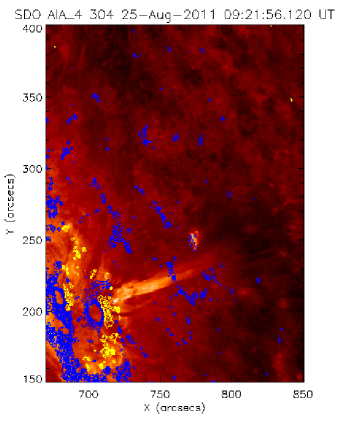
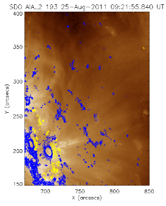
Figure 1: SDO/AIA 193 Å (right, yellow-brown map for 1.0 MK plasma) and 304 Å (left, red-temperature map for 0.1 MK plasma) EUV images overlaid by HMI magnetic field contours of maximum level $\pm$800 G. Yellow (blue) contours show positive (negative) polarity of the magnetic field. The surge origin is accompanied by heating above its foot-point. The observed surge is clearly evident in He II 304 Å filter that is sensitive to the low temperature plasma of 0.1 MK. Some heated part of the surge especially near its base up-to the height of 20 Mm, is also evident in the coronal filters (e.g., 193 Å ) that are sensitive to the plasma temperature around 1.0 MK. The surge is originated from the western boundary of the positive polarity situated in the North-West direction of the big sunspot with negative polarity as represented by the blue circular contour at X = 700$"$, Y = 200$"$.

We use an image sequence of a solar surge in AR11271 on 25 August 2011 during 09:11–09:31 UT as observed in the 304 Å  and 193 Å  filters, which represent 10⁵ K and 10⁶ K plasma, respectively. The surge originated near the western boundary of AR11271 as shown in Fig. 1. These images are overlaid by SDO/HMI magnetic field contours at a level of $\pm$800 G : yellow (blue) stays for positive (negative) polarity.It is clearly evident that the surge occurred near a positive polarity region (yellow) in the north-west side of a big negative polarity spot (shown by blue circle). The surge plasma mostly emits in the 304 Å filter sensitive to the plasma temperature around $\sim$10⁵ K , but does not show much emission in the coronal filter. However, some emission in the hotter coronal channel is visible up to the height of 20 Mm from the foot point of the surge (cf., right panel of Fig. 1). Therefore, the surge consists of multi-temperature plasma.

2.1 Kinematics of the Surge

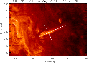
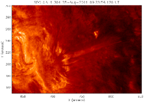
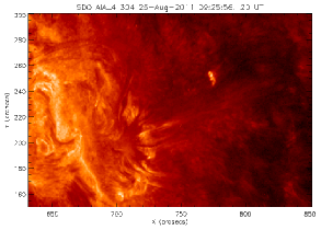
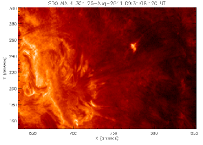
Figure 2: SDO/AIA 304 Å time sequence of a surge propagation higher into the corona from the boundary of an active region NOAA AR11271. The surge fades gradually with time, and the material tries to settle down due to gravity. Horizontal and vertical dotted lines on the snapshot of 09:21 UT show the two paths along which the Distance-Time measurements have been made.

Fig. 2 represents the spatio-temporal evolution of the surge material using the sub-field data. It is clear that the surge is being activated at 09:11 UT near the western boundary of NOAA AR11271, and faded around 09:21 UT. The observed surge was not associated with the recurrent spray surge activity in AR11271 (Kayshap et al., 2012). This image sequence shows that the surge reaches upto a projected height of $\approx$65 Mm in $\approx$660 s. The terminal speed of the surge is found to be $\approx$100 km s^-1. This surge is well collimated with a maximum width of $\approx$7 Mm and does not show any significant lateral expansion. Its down falling time is $\approx$500 s in which it also faded gradually. Top-panel of Fig. 3 shows the distance-time measurement along the observed surge. It is evident that the denser core material of the surge first rises up and then decelerates. Some fainter and less denser plasma reaches much higher into the solar atmosphere, and falls freely thereafter. The distance-time map across the surge at a particular height around $\approx$15 Mm is shown in the bottom panel. The radiance periodicity is observed on 3.0 min time-scale, which may be the signature of the periodic enhancement of mass density in the surge. This may provide the clues about the periodic driver of the surge, which will be discussed in detail in Sec. 3. It is also possible that the periodicity of 3.0 min near the surge base may be due to the swirling motion as recently observed in spectroscopic data (e.g., Wedemeyer-Böhm et al., 2012b; De Pontieu et al., 2012, and references cited therein). However, such small-scale motion is below the detection limit in our data. Moreover, the radiance oscillations occur higher in the transition region, and therefore, in the present case it may be the most likely evidence of the periodic signature of the arrival of slow shocks in the upper chromosphere/transition region.

2.2 Estimations of the Average Temperature and Density of the Surge

In the present section, we carried out emission measure and temperature distribution analysis, as well as the tracing and estimation of density along the surge by extensively using the automated method developed by Aschwanden et al. (2011). Understanding such plasma properties provide more clues about the driver of the surge, while comparing with the numerical results. SDO/AIA data provides information of the emission measure and estimation of the average density and temperature (Aschwanden et al., 2011). We use full-disk SDO/AIA in all EUV channels at the time of the maximum rise of the surge around 09:22 UT on 25 August, 2011. We calibrate and clean the data using aia_prep subroutine of SSW IDL as well as co-align the AIA images as observed in various AIA filters by using the co-alignment test as described by Aschwanden et al. (2011).

Using the automated code developed by Aschwanden et al. (2011), we obtain emission measure and temperature maps for six AIA filter full-disk and co-aligned images (304 Å, 171 Å, 193 Å, 94 Å, 335 Å, 211 Å) in the temperature between 0.5-9.0 MK. The emission measure map in the top-left panel of Fig. 4 shows that the surge has significant emissions from its denser core part. The emissions from its leading edge is comparatively low. Top-right panel of Fig. 4 shows the distribution of temperature in and around the surge location. It is evident that heating is confined near its foot-point. Greenish-yellow regions represent the highest temperature in and around the footpoint of the surge. The reddish region shows the plasma at the base of the surge with a temperature of 6.2-6.3 MK. Above the heated area near the base of the surge, the cool plasma is maintained at sub-coronal temperatures as represented by blue-black colors. It is also mixed with the comparatively hot plasma. The leading edge of the surge is, however, maintained at comparatively high coronal temperatures. The heating near the base of the surge probably drives it, and the cool plasma moves behind the hot plasma at its leading edge. It is also mixed with the hot plasma, and constitutes the multi-temperature surge.

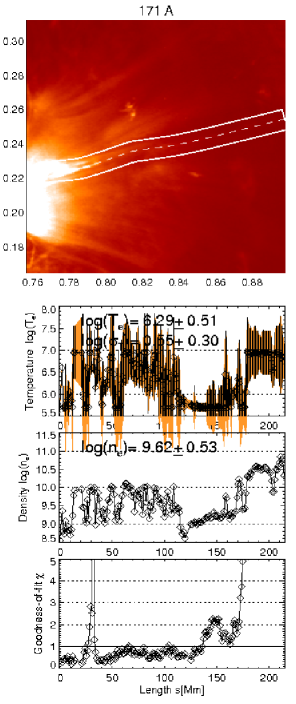
Figure 5: The AIA 171 Å image (top-panel) displays the sub-field containing the surge and its overlying diffuse corona. The image axes are scaled as a fraction of the solar radius. This panel shows the 171 Å image in which the box shows the area along the surge and its overlying diffuse corona along which the physical parameters are evaluated. The estimated plasma properties, e.g., the integrated density, temperature along the surge (dashed-line) during its maximum rise are displayed in two consecutives middle-panels.

Using the automated procedure (Aschwanden et al., 2011), we trace the loop segments and surge in the co-spatial and co-temporal images of various wavelengths of SDO/AIA data. The input free parameters for this automated tracing of the surge is summarized in Table 1. The bottom panel of Fig. 4 shows that the surge material is erupting along open field lines, indicated by white arrow, from the western part of active region boundary. The surge consists of multi-temperature plasma. The contribution of cool surge plasma (T=0.1 MK) as evident in 304 Å channel, is represented by yellow colour. For the estimation of the plasma properties (temperature and density) along the surge material and its overlying diffuse corona, we trace the larger segment of this coronal structure using another set of free parameters (cf., Table 1) and implement the best forward fit of the possible DEM solutions. We choose this set of free parameters on the basis of trial and error, and it gives the best DEM forward fit in the case of 171 Å fluxes at each pixel of the considered region around the surge and its overlying atmosphere. In Fig. 5, the estimated density and temperature are displayed. The chi-square of the estimation in the forward modeling is good-enough up to 70 Mm along the surge as well as upto 140 Mm in its overlying diffuse corona. The average temperature and density of the surge material are respectively 2.0 MK and 4.1$\times$10⁹ cm^-3. We can estimate these physical parameters in all the traced structures in all AIA channels. However, we display the best fit results of the estimation of the density and temperature along the surge and its overlying corona in 171Å  channel as shown in Fig. 5.

2.3 SDO/HMI Investigations of the Magnetic Field Properties at the Base of the Surge

The surge occurred at the north-western side of the big sunspot with negative polarity. It was located at the outer layer of a positive polarity region (cf., snapshot on 09:00 UT in Fig. 6). The surge is shown as intensity contour (blue) of co-aligned AIA data on HMI snapshot of 09:21 UT in Fig. 6. The morphology of the origin site of the observed surge is almost similar to that observed recently by Uddin et al. (2012) in association with the recurrent surges from NOAA 10884 on 25 October 2003. However, we do not observe any strong signature of the magnetic field annihilation as well as moving magnetic features (MMFs) in our present observational data as previously observed by Uddin et al. (2012). Therefore, we infer that the observed surge may not be triggered by strong photospheric magnetic field activities. It is evident that tiny negative magnetic polarities have been evolved near the surge location, as well as the major positive polarity region has shown some areal enhancement towards the western direction. Therefore, such rearrangements of the magnetic polarities around the surge region may produce more complexity in the overlying magnetic flux-tubes (Roy, 1973; Canfield et al., 1996), e.g., in low-lying loops and an arch crossing near the base of the surge (cf., 09:11 UT AIA 304 Å snapshot of Fig. 2; HMI-AIA snapshot on 09:20 UT in Fig. 6). Therefore, the chromospheric reconnection between the open field lines as well as surrounding closed fields may trigger the surge. The localized brightening and heating at the same location is evident where dark arch type flux-tube and low-lying closed loops are crossing near the surge base (cf., 09:11 UT snapshot of Fig. 2, and right panel of Fig. 4), which may generate the thermal pulse probably triggering the observed plasma perturbations. In the next section, in support of the present observational base-line of the triggering of the surge due to chromospheric heating, we devise a numerical model with implementation of VAL-C atmosphere and a thermal pulse as an initial trigger, which re-produce the observations closely.

3 A NUMERICAL MODEL FOR THE PULSE-DRIVEN SOLAR SURGE

To reproduce the observed surge, our model system assumes a gravitationally-stratified solar atmosphere that is described by the ideal two-dimensional (2D) MHD equations:

$${{\partial\varrho}\over{\partial t}}+\nabla\cdot(\varrho{\bf V})=0\,,$$ (1)

$$\varrho{{\partial{\bf V}}\over{\partial t}}+\varrho\left({\bf V}\cdot\nabla\right){\bf V}=-\nabla p+\frac{1}{\mu}(\nabla\times{\bf B})\times{\bf B}+\varrho{\bf g}\,,$$ (2)

$${\partial p\over\partial t}+\nabla\cdot(p{\bf V})=(1-\gamma)p\nabla\cdot{\bf V}\,,$$ (3)

$${{\partial{\bf B}}\over{\partial t}}=\nabla\times({\bf V}\times{\bf B})\,,\hskip 8.53581pt\nabla\cdot{\bf B}=0\,.$$ (4)

Here ${\varrho}$, ${\bf V}$, ${\bf B}$, $p=\frac{k_{\rm B}}{m}\varrho T$, $T$, $\gamma=5/3$, ${\bf g}=(0,-g)$ with its value $g=274$ m s^-2, $m$, $k_{\rm B}$, are respectively the mass density, flow velocity, magnetic field, gas pressure, temperature, adiabatic index, gravitational acceleration, mean particle mass, and Boltzmann’s constant. It should be noted that we do not invoke the radiative cooling and thermal conduction in our model for simplicity reasons since we simulate the cool surge ejecta in the solar atmosphere.

3.1 Equilibrium configuration

We assume that at its equilibrium the solar atmosphere is still (${\bf V}_{\rm e}={\bf 0}$) with a force-free magnetic field,

$$(\nabla\times{\bf B}_{\rm e})\times{\bf B}_{\rm e}={\bf 0}\ ,$$ (5)

such that it satisfies a current-free condition, $\nabla\times{\bf B}_{\rm e}={\bf 0}$, and it is specified by the magnetic flux function, $A$, as

$${\bf B}_{\rm e}=\nabla\times(A\hat{\bf z})\,.$$ (6)

Here the subscript ’${\rm e}$’ corresponds to equilibrium quantities. We set an arcade magnetic field by choosing

$$A(x,y)=B_{\rm 0}{\Lambda}_{\rm B}\cos{(x/{\Lambda}_{\rm B})}{\rm exp}[-(y-y_{\rm r})/{\Lambda}_{\rm B}]\,$$ (7)

with $B_{\rm 0}$ being the magnetic field at $y=y_{\rm r}$, and the magnetic scale-height is

$${\Lambda}_{\rm B}=\frac{2L}{\pi}\,.$$ (8)

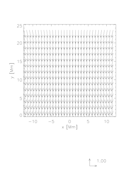
Figure 7: Equilibrium profile of solar temperature (top panel) and magnetic field vectors (bottom panel). The magnetic field is expressed in units of 44 gauss and a part of the simulation region is displayed.

We set and hold fixed $L=100$ Mm. For such choice the magnetic field vectors are weakly curved (Fig. 7, bottom panel).

As a result of Eq. (5) the pressure gradient is balanced by the gravity force,

$$-\nabla p_{\rm e}+\varrho_{\rm e}{\bf g}={\bf 0}\,.$$ (9)

With the ideal gas law and the $y$-component of Eq. (9), we arrive at

$$p_{\rm e}(y)=p_{\rm 0}~{}{\rm exp}\left[-\int_{y_{\rm r}}^{y}\frac{dy^{{}^{\prime}}}{\Lambda(y^{{}^{\prime}})}\right]\,,\hskip 8.53581pt\varrho_{\rm e}(y)=\frac{p_{\rm e}(y)}{g\Lambda(y)}\,,$$ (10)

where

$$\Lambda(y)=\frac{k_{\rm B}T_{\rm e}(y)}{mg}$$ (11)

is the pressure scale-height, and $p_{\rm 0}$ denotes the gas pressure at the reference level that we choose in the solar corona at $y_{\rm r}=10$ Mm.

We take an equilibrium temperature profile $T_{\rm e}(y)$ for the solar atmosphere derived from the VAL-C atmospheric model of Vernazza et al. (1981). Having specified $T_{\rm e}(y)$ (see Fig. 7, top panel) with Eq. (10) we obtain the corresponding gas pressure and mass density profiles.

The transition region (TR) is located at $y\simeq 2.7$ Mm. Above the TR we assume an extended solar corona. Below the solar chromosphere, the temperature minimum is located at $y\simeq 0.9$ Mm.

3.2 Perturbations

We initially perturb the equilibrium impulsively by a Gaussian pulse in a gas pressure viz.,

$$p(x,y,t=0)=p_{\rm e}(y)+\\ p_{\rm e}(y)A_{\rm p}\exp\left[-\frac{(x-x_{\rm 0})^{2}}{w_{\rm x}^{2}}-\frac{(y-y_{\rm 0})^{2}}{w_{\rm y}^{2}}\right]\,.$$

Here $A_{\rm p}$ is the amplitude of the pulse, $(x_{\rm 0},y_{\rm 0})$ is its initial position and $w_{\rm x}$, $w_{\rm y}$ denote its widths along the $x$- and $y$-directions, respectively. We set and hold fixed $A_{\rm p}=80$, $x_{\rm 0}=0$ Mm, $y_{\rm 0}=1.75$ Mm, $w_{\rm x}=2.25$ Mm, and $w_{\rm y}=0.2$ Mm.

3.3 Results of the Numerical Simulations

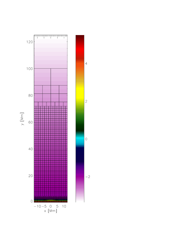
Figure 8: The grid system with block boundaries represented by solid lines as adopted in the simulation. The initial pressure perturbation of the system is displayed by the horizontally elongated patch at a location $(0Mm,1.75Mm)$.

Equations (1)-(4) are solved numerically using the FLASH code (Lee & Deane, 2009; Fryxell et al., 2000). This code uses a second-order unsplit Godunov solver with various slope limiters and Riemann solvers, as well as adaptive mesh refinement (AMR). We set the simulation box of $(-12.5,12.5)\,\times(0,125)\,$ Mm² along the $x$- and $y$-directions (Fig. 8, bottom panel) and set and hold fixed all plasma quantities at all boundaries of the simulation region to their equilibrium values which are given by Eqs. (6) and (10). These fixed boundary conditions performed much better than transparent boundaries, leading only to negligibly small numerical reflections of wave signals from these boundaries.

In our modeling, we use an AMR grid with a minimum (maximum) level of refinement set to $4$ ($7$) (Fig 8). The refinement strategy is based on controlling numerical errors in mass density, which results in an excellent resolution of steep spatial profiles and greatly reduces numerical diffusion at these locations.

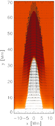
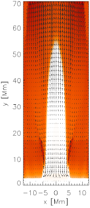
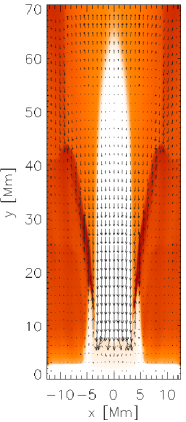
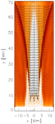
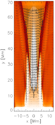
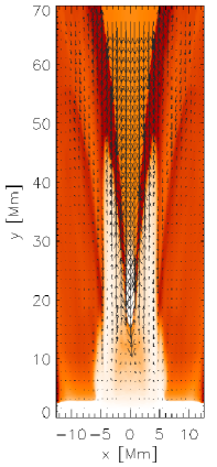
Figure 9: Temporal snapshots of a simulated surge. The temperature (colour maps) profiles at $t=200$ s, $t=400$ s, $t=600$ s, $t=800$ s, $t=1000$ s, and $t=1200$ s (from top to bottom). Temperature is drawn in units of $1$ MK as shown in the colour bar, which is common to all the panels. The velocity vector unit is 150 km s^-1.

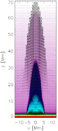
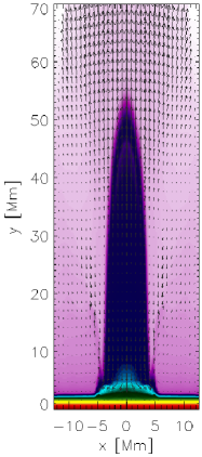
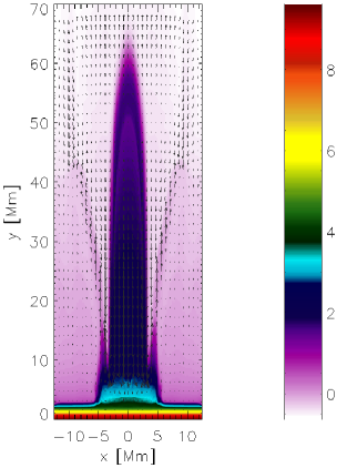
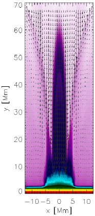
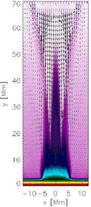
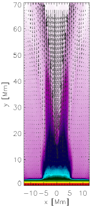
Figure 10: Temporal snapshots of a simulated surge. The density (colour maps) profiles at $t=200$ s, $t=400$ s, $t=600$ s, $t=800$ s, $t=1000$ s, and $t=1200$ s (from top to bottom). Density is drawn in the units of 10^-12 kg m^-3 as shown in the colour bar, which is common to all the panels. The velocity vector unit is 150 km s^-1.

Fig. 9 displays the spatial profiles of the plasma temperature (color maps) and velocity (arrows) resulting from the initial pulse of Eq. (3.2), which splits into counter-propagating pulse trains. The downward propagating part is reflected from the dense ambient plasma of the photosphere. This reflected part lags behind the originally upward propagating pulses, which become slow shocks. Because the plasma is initially pushed upward, the under-pressure results in the region below the initial pulse. This under-pressure sucks up comparatively cold chromospheric plasma, which lags behind the shock front at higher temperature. As a result, the pressure gradient force works against gravity and forces the chromospheric material to arrive into the solar corona in form of a rarefaction wave. At $t=200$ s this shock reaches the altitude of $y\simeq 65$ Mm and the cold plasma edge is located at $y\simeq 35$ Mm, which is below the slow shock. The reason for the material being lifted up is the rarefaction of the plasma behind the shock front, which leads to low pressure there. The next snapshot (top middle panel) is drawn for $t=400$ s. At this time the chromospheric plasma is located below at $y\simeq 55$ Mm. At the next moment, $t=600$ s (top right panel) the chromospheric plasma shows its developed phase, reaching the level of $y=65$ Mm, which approximately matches the observational data of Fig. 2 (top right panel). The cool surge slows down while propagating upward. At $t=800$ s it arrives at the level of $y\simeq 70$ Mm and subsequently the surge already subsides being attracted by gravity (bottom panels). At the subsiding stage the heated fine structures develop as a result of interaction between the down-falling plasma. During the evolution of the surge, the comparatively hot plasma is evident near the base of the simulated surge that qualitatively matches the observations. The leading front of the slow shock moving above the cool surge plasma may also leave some traces in the overlying diffused quiet-Sun atmosphere evident in the coronal filters (cf., right panel of Fig.1). However, the less denser and diffused overlying quiet-Sun may not be visible as a tracer of a slow shock front. The temporal evolution of the density reveals that the surge is denser near its base, while the density decreases with the height (Fig. 10). This is consistent with the observational data.

4 DISCUSSIONS AND CONCLUSION

In the present paper, we study the kinematics and plasma properties of the solar surge triggered in AR11271 on 25 August, 2011. We also performed a 2 D numerical simulation using VAL-C model of the solar atmosphere as initial condition and the FLASH code (Fryxell et al., 2000), which approximately reproduce the dynamics of the observed cool surge. The surge rises vertically from its origin site up to a height $\approx$65 Mm with a terminal velocity of $\approx$100 km s^-1, and thereafter falls and fades gradually within its total life time of $\approx$20 min. We also measure the temperature and density distribution of the observed surge during its maximum rise, and its average temperature and density are respectively $2.0$ MK and $4.1\times$10⁹ cm^-3. We do not get any strong evidence of the photospheric magnetic field activity (i.e., MMFs, flux-emergence, field annihilation, etc) in support of the formation of the observed surge. The surge is most likely found to be driven by magnetic reconnection generated thermal energy in the chromosphere.

The numerical simulations exhibit a general scenario of rising and subsequently down-falling/fading of the observed surge with a number of observational features such as its height and width, ejection, approximate rising time-scale, and average rising velocity that are close to the observational data. The heated fine structures at the base of the surge are also matching well both in the observations and theory. The temperature distribution (Fig. 4) shows that the significant amount of cool plasma expands along the surge, while its leading edge is maintained at coronal temperatures. This scenario matches qualitatively with our simulation results when the comparatively cooler core plasma of surge lags behind the high temperature slow shock. The kinematical estimations of the surge (Fig. 3) also reveals the acceleration of the surge material and its subsequent free fall due to gravity thereafter, which also matches well the simulation results. However, some parts of the comparison between the numerical and observational data are approximate and only qualitative. This mismatch may result from simplified profiles of the parameters in our numerical model. Moreover, the real surge was excited in more complex plasma and magnetic field conditions at the boundary of AR11271.

It is reported in literature that if the height of the energy release site is less (greater) than a critical height then the jet will be driven by crest shocks (directly by the pressure gradient force generated by explosion) (Shibata et al., 1982). However, this minimum critical height in the solar atmosphere depends upon the strength of pressure enhancement in time at the energy release site. For the larger pressure enhancement, this height will be lower and vice versa. Under the conditions when the energy release site is higher in the solar atmosphere, the surge material may be accelerated by the ${\bf j}{\times}{\bf B}$ force as a result of reconnection (Yokoyama & Shibata, 1995, 1996) as observed by Nishizuka et al. (2008). Therefore, the surge dynamics may not be so simple like a thermal pulse driven jet, and magnetic forces may also play some role in its formation. If the reconnection and thus the energy release site occurs in the lower chromosphere, any ${\bf j}{\times}{\bf B}$ force driven flow may generate slow mode MHD wave/shock which eventually accelerates the jet in the upper chromosphere and transition region (Shibata et al., 1982). We consider the energy release site and the triggering by the thermal pulse at $y$=1.75 Mm above the photosphere, and its amplitude A_p=80 times larger than the ambient gas pressure. In our case, A_p is beyond the parameters considered by Shibata et al. (1982). We aim to perform some parametric studies in order to compare numerical results with the findings of Shibata et al. (1982), which will be devoted to our potential future studies. However, it is noteworthy that the numerical model we devised, is an extension of the 1D model of Shibata et al. (1982). We adopted the temperature profile and a curved magnetic field in the MHD regime, therefore our 2D model represents a natural extension of the hydrodynamic model of Shibata et al. (1982) in simulating the cool jet.

5 Acknowledgments

We acknowledge the constructive suggestions of the reviewer, which considerably improve our manuscript, use of automated DEM and temperature analysis of solar structures developed by Prof. Markus Aschwanden, LMSAL, USA, and the use of the SDO/AIA observations for this study. The FLASH code has been developed by the DOE-supported ASC/Alliance Center for Astrophysical Thermonuclear Flashes at the University of Chicago. This work has been supported by a Marie Curie International Research Staff Exchange Scheme Fellowship within the 7th European Community Framework Program (K.M.). PK acknowledges UMCS, Lublin, Poland for the visit grant in 2011 where the part of the work has been executed. AKS acknowledges Shobhna Srivastava for patient encouragement during the work. AKS also thanks Prof. K. Shibata for his valuable suggestions during the discussion on the simulation of solar jets. KM thanks Kamil Murawski for his assistance in drawing numerical data.

Table 1: The Summary of Input Free Parameters

	Half	Threshold level	Min filling	Output	Minimum	Max traced	Min curvature
	Width	in standard	factor	resolution	length	structures	radius
		flux deviation
To trace the surge	2 pixels	1.0	0.35	5.0	0.01	10,000	25
To estimate the plasma properties	10 pixels	1.0	0.15	5.0	0.04	10,000	60

 

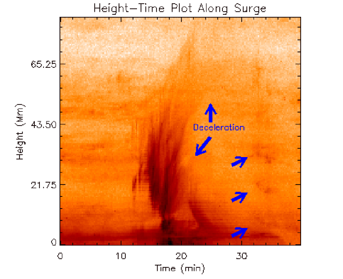
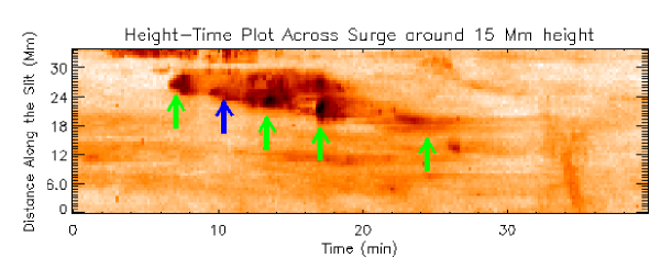
Figure 3: The height-time plots : (i) Along the solar surge using He II 304 Å data (top) where the distance is measured along the slit chosen along the surge; (ii) Across the surge at a height of $\approx$15 Mm from its base (bottom) where the distance is measured along the slit chosen across the surge. The positions of both the slits are shown over the 09:21 304 Å snapshot in Fig. 2.

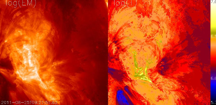
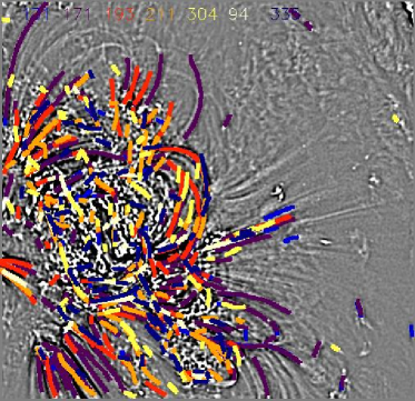
Figure 4: The Emission Measure (EM) map (top-left) and temperature map (top-right panel) : Evidence of the multi-temperature plasma forming the surge. The lower part of the surge consists of cool plasma, while the leading edge exhibits coronal temperatures. Bottom panel shows the automated tracing of the plasma threads as visible at various temperatures along the open field lines of the surge as shown by arrow using the methodology of Aschwanden et al. (2011). Colour codes for the emitting plasma in different AIA channels are shown at the top of this snapshot.

Figure 6: Co-aligned SDO/HMI time sequence of the photospheric magnetic field near the origin of the surge. The blue surge is shown as intensity contour on HMI snapshot of 09:21 UT. The blue loop arches on both the sides of the surge may cause possible reconnection at its base to heat and subsequently launch a thermal pulse for its acceleration.

References

- Aschwanden et al. (2011) Aschwanden, M. J., Boerner, P., Schrijver, C. J., & Malanushenko, A. 2011, Sol. Phys., 384
- Bohlin et al. (1975) Bohlin, J. D., Vogel, S. N., Purcell, J. D., Sheeley, N. R., Jr., Tousey, R., & Vanhoosier, M. E. 1975, ApJ, 197, L133
- Brooks et al. (2007) Brooks, D. H., Kurokawa, H., & Berger, T. E. 2007, ApJ, 656, 1197
- Canfield et al. (1996) Canfield, R. C., Reardon, K. P., Leka, K. D., Shibata, K., Yokoyama, T., & Shimojo, M. 1996, ApJ, 464, 1016
- Chae et al. (1999) Chae, J., Qiu, J., Wang, H., & Goode, P. R. 1999, ApJ, 513, L75
- Cirtain et al. (2007) Cirtain, J. W., et al. 2007, Science, 318, 1580
- Culhane et al. (2007) Culhane, L., et al. 2007, PASJ, 59, 751
- De Pontieu et al. (2012) De Pontieu, B., Carlsson, M., Rouppe van der Voort, L. H. M., Rutten, R. J., Hansteen, V. H., & Watanabe, H. 2012, ApJ, 752, L12
- De Pontieu et al. (2004) De Pontieu, B., Erdélyi, R., & James, S. P. 2004, Nature, 430, 536
- De Pontieu et al. (2007a) De Pontieu, B., Hansteen, V. H., Rouppe van der Voort, L., van Noort, M., & Carlsson, M. 2007a, ApJ, 655, 624
- De Pontieu et al. (2007b) De Pontieu, B., et al. 2007b, PASJ, 59, 655
- De Pontieu et al. (2011) De Pontieu, B., et al. 2011, Science, 331, 55
- De Pontieu et al. (2007c) De Pontieu, B., et al. 2007c, Science, 318, 1574
- Filippov et al. (2009) Filippov, B., Golub, L., & Koutchmy, S. 2009, Sol. Phys., 254, 259
- Fryxell et al. (2000) Fryxell, B., et al. 2000, ApJS, 131, 273
- Gaizauskas (1996) Gaizauskas, V. 1996, Sol. Phys., 169, 357
- Hansteen et al. (2006) Hansteen, V. H., De Pontieu, B., Rouppe van der Voort, L., van Noort, M., & Carlsson, M. 2006, ApJ, 647, L73
- Innes et al. (1997) Innes, D. E., Inhester, B., Axford, W. I., & Wilhelm, K. 1997, Nature, 386, 811
- Jiang et al. (2007) Jiang, Y. C., Chen, H. D., Li, K. J., Shen, Y. D., & Yang, L. H. 2007, A&A, 469, 331
- Kamio et al. (2010) Kamio, S., Curdt, W., Teriaca, L., Inhester, B., & Solanki, S. K. 2010, A&A, 510, L1
- Katsukawa et al. (2007) Katsukawa, Y., et al. 2007, Science, 318, 1594
- Kayshap et al. (2012) Kayshap, P., Srivastava, A., & Murawski, K. 2012, Sol. Phys., 386, , in preparation
- Lee & Deane (2009) Lee, D., & Deane, A. E. 2009, Journal of Computational Physics, 228, 952
- Lemen et al. (2012) Lemen, J. R., et al. 2012, Sol. Phys., 275, 17
- Liu & Kurokawa (2004) Liu, Y., & Kurokawa, H. 2004, ApJ, 610, 1136
- Liu et al. (2005) Liu, Y., Su, J. T., Morimoto, T., Kurokawa, H., & Shibata, K. 2005, ApJ, 628, 1056
- Madjarska et al. (2009) Madjarska, M. S., Doyle, J. G., & de Pontieu, B. 2009, ApJ, 701, 253
- Morton et al. (2012) Morton, R. J., Srivastava, A. K., & Erdélyi, R. 2012, A&A, 542, A70
- Murawski et al. (2011) Murawski, K., Srivastava, A. K., & Zaqarashvili, T. V. 2011, A&A, 535, A58
- Murawski & Zaqarashvili (2010) Murawski, K., & Zaqarashvili, T. V. 2010, A&A, 519, 8
- Nishizuka et al. (2008) Nishizuka, N., Shimizu, M., Nakamura, T., Otsuji, K., Okamoto, T. J., Katsukawa, Y., & Shibata, K. 2008, ApJ, 683, L83
- Pariat et al. (2010) Pariat, E., Antiochos, S. K., & DeVore, C. R. 2010, ApJ, 714, 1762
- Roy (1973) Roy, J. R. 1973, Sol. Phys., 28, 95
- Schmieder et al. (1994) Schmieder, B., Golub, L., & Antiochos, S. K. 1994, ApJ, 425, 326
- Schou et al. (2012) Schou, J., et al. 2012, Sol. Phys., 275, 229
- Shibata et al. (2007) Shibata, K., et al. 2007, Science, 318, 1591
- Shibata et al. (1982) Shibata, K., Nishikawa, T., Kitai, R., & Suematsu, Y. 1982, Sol. Phys., 77, 121
- Srivastava & Murawski (2011) Srivastava, A. K., & Murawski, K. 2011, A&A, 534, A62
- Sterling (2000) Sterling, A. C. 2000, Sol. Phys., 196, 79
- Sterling et al. (1993) Sterling, A. C., Shibata, K., & Mariska, J. T. 1993, ApJ, 407, 778
- Uddin et al. (2012) Uddin, W., Schmieder, B., Chandra, R., Srivastava, A. K., Kumar, P., & Bisht, S. 2012, ApJ, 752, 70
- Vernazza et al. (1981) Vernazza, J. E., Avrett, E. H., & Loeser, R. 1981, ApJS, 45, 635
- Wedemeyer-Böhm et al. (2012a) Wedemeyer-Böhm, S., Scullion, E., Steiner, O., Rouppe van der Voort, L., de La Cruz Rodriguez, J., Fedun, V., & Erdélyi, R. 2012a, Nature, 486, 505
- Wedemeyer-Böhm et al. (2012b) Wedemeyer-Böhm, S., Scullion, E., Steiner, O., Rouppe van der Voort, L., de La Cruz Rodriguez, J., Fedun, V., & Erdélyi, R. 2012b, Nature, 486, 505
- Yokoyama & Shibata (1995) Yokoyama, T., & Shibata, K. 1995, Nature, 375, 42
- Yokoyama & Shibata (1996) Yokoyama, T., & Shibata, K. 1996, PASJ, 48, 353
- Yoshimura et al. (2003) Yoshimura, K., Kurokawa, H., Shimojo, M., & Shine, R. 2003, PASJ, 55, 313