A multiprecision C++ library for matrix-product-state simulation of quantum computing: Evaluation of numerical errors

Abstract

The time-dependent matrix-product-state (TDMPS) simulation method has been used for numerically simulating quantum computing for a decade. We introduce our C++ library ZKCM_QC developed for multiprecision TDMPS simulations of quantum circuits. Besides its practical usability, the library is useful for evaluation of the method itself. With the library, we can capture two types of numerical errors in the TDMPS simulations: one due to rounding errors caused by the shortage in mantissa portions of floating-point numbers; the other due to truncations of nonnegligible Schmidt coefficients and their corresponding Schmidt vectors. We numerically analyze these errors in TDMPS simulations of quantum computing.

1 Introduction

Simulations of time-evolving quantum states using a matrix-product-state (MPS) [1] representation have been widely used in a variety of physical systems [2, 3]. We have been developing a C++ library, named ZKCM_QC [4], for multiprecision time-dependent MPS (TDMPS) simulations of quantum computing using Vidal’s representation [5] for MPS. Here, we define the precision by the length of a mantissa portion for each floating point number.

Let us begin with a brief description of conventions. We employ the computational basis $\{|0\rangle,|1\rangle\}^{n}$ for $n$-qubit quantum states, where $|0\rangle=\left(\begin{array}[]{cc}1&0\end{array}\right)^{\rm T}$ and $|1\rangle=\left(\begin{array}[]{cc}0&1\end{array}\right)^{\rm T}$. An $n$-qubit quantum state is represented as $|\Psi\rangle=\sum_{i_{0}\cdots i_{n-1}=0\cdots 0}^{1\cdots 1}c_{i_{0}\cdots i_{n-1}}|i_{0}\cdots i_{n-1}\rangle$ with complex amplitudes $c_{i_{0}\cdots i_{n-1}}$. In this paper, we employ the following MPS form [5, 6] of the state, for our TDMPS simulations.

$$\begin{array}[]{rl}|\Psi\rangle=&\sum_{i_{0}\cdots i_{n-1}=0\cdots 0}^{1\cdots 1}\biggl{[}\sum_{v_{0}=0}^{m_{0}-1}\sum_{v_{1}=0}^{m_{1}-1}\cdots\sum_{v_{n-2}=0}^{m_{n-2}-1}Q_{0}(i_{0},v_{0})V_{0}(v_{0})Q_{1}(i_{1},v_{0},v_{1})V_{1}(v_{1})\cdots\\ &Q_{s}(i_{s},v_{s-1},v_{s})V_{s}(v_{s})\cdots V_{n-2}(v_{n-2})Q_{n-1}(i_{n-1},v_{n-2})\biggr{]}|i_{0}\cdots i_{n-1}\rangle,\end{array}$$ (1)

where we use tensors $\{Q_{s}\}_{s=0}^{n-1}$ with parameters $i_{s},v_{s-1},v_{s}$ ($v_{-1}$ and $v_{n-1}$ are excluded) and $\{V_{s}\}_{s=0}^{n-2}$ with parameter $v_{s}$; $m_{s}$ is a suitable number of values for $v_{s}$, with which the state is represented precisely or well approximated. [Tensor $V_{s}(v_{s})$ stores the Schmidt coefficients for the splitting between the $s$th site and the $(s+1)$th site.]

With the MPS form, the cost to update data in accordance with a time evolution is reduced considerably in comparison to the brute-force method. We have only to update tensors corresponding to the sites under the influence of a unitary operator for each step. The cost to simulate an evolution by a single unitary operation $\in{\rm U}(4)$ acting on some consecutive sites is $O(m_{\rm max}^{3})$ floating-point operations where $m_{\rm max}$ is the largest value of $m_{s}$ among the sites $s$ [5]. The total cost of a TDMPS simulation thus grows polynomially in the largest Schmidt rank among those for the splittings, which highly depends on the instance of the problem of one’s concern. (Here, each splitting we consider is, of course, a bipartite splitting between consecutive sites.)

The TDMPS simulation method in double precision [i.e., (52+1)-bits-long mantissa for a floating point number] has already been used commonly in the community of computational physics [7]. There are, however, known cases for general computational methods where more accurate computation is needed to obtain a reliable results describing physical phenomena [8]. Accumulations of rounding errors of basic arithmetic operations are the main cause in such cases. This should be true also in TDMPS simulations of quantum computing where many matrix diagonalizations are involved unless the depth of quantum circuits is very small. Besides the precision of basic operations, another factor of losing accuracy is the truncation of Schmidt coefficients. When many of Schmidt coefficients are nonnegligible at a certain step of a TDMPS simulation, imposing a threshold to the number of Schmidt coefficients for each splitting may truncate out important data affecting simulation results [9]. So far truncations of nonvanishing Schmidt coefficients have been uncommon and the largest Schmidt rank and its upper bound in the absence of truncations have been of main concern when MPS and related data structures are used for handling quantum and/or classical computational problems [5, 11, 12, 6, 13, 14, 15, 16, 17]. This is in contrast to MPS and TDMPS simulations in condensed matter physics where truncations are very commonly employed [18].

In this report, we evaluate numerical errors in actual TDMPS simulations of quantum computing. We first begin with a brief introduction to the ZKCM_QC library in section 2. Then we conduct numerical evaluations in section 3: an error due to precision shortage is investigated in section 3.1 and that due to truncations of Schmidt coefficients is investigated in section 3.2. We discuss and summarize obtained results in sections 4 and 5, respectively.

2 ZKCM_QC library

The ZKCM_QC library has been developed as a C++ library for TDMPS simulations of quantum computing with an emphasis on multiprecision computation. It is an extension package of the ZKCM library [19] which uses the GMP [20] and MPFR [21] libraries for basic arithmetic operations. We briefly explain the usage of the ZKCM_QC library.

The library can be installed by the standard process: “./configure”, “make”, and “make install” in any Unix-like system with GNU tools. Once it is installed, a user will write a C++ program using the header file “zkcm_qc.hpp” and compile the program with the library flags “-lzkcm_qc -lzkcm -lmpfr -lgmp -lgmpxx -lm” using a C++ compiler.

In the main part of a program, a user will firstly specify the default precision. For example “zkcm_set_default_prec(256);” will set the default precision to 256 bits. Then, a user will call a constructor of the class “mps” to create the object of an MPS kept in the form of (1). For example, “mps M(5);” will generate an object keeping the data of $|0_{0}0_{1}0_{2}0_{3}0_{4}\rangle$ in the MPS form. Then a user will apply certain unitary operations by using some member functions of the class, such as “applyU” and “applyU8” with predefined and/or user-defined unitary matrices. For example, “M.applyU(tensor2tools::Hadamard, 2);” applies an Hadamard gate $H=\left(\begin{array}[]{cc}1&1\\ 1&-1\end{array}\right)/\sqrt{2}$ to qubit $2$. For another example, “M.applyU(tensor2tools::CNOT, 2, 4);” applies the CNOT gate to qubits $2$ and $4$ that are the control bit and the target bit, respectively. Here, CNOT is a conditional bit flip; the target bit is flipped when the control bit is in $|1\rangle$. There are other member functions for unitary operations. For instance, “CCNOT” is used for a CCNOT operation; “M.CCNOT(0, 2, 4);” applies a bit flip on qubit $4$ under the condition that qubits $0$ and $2$ are both in $|1\rangle$. In addition, it is possible to simulate a projective measurement by calling the member function “pmeasure”. For example, “int event = M.pmeasure(zkcm_matrix("[1,0;0,-1]"), 2, -1);” will simulate a projective measurement on qubit $2$ with the observable Pauli $Z$, as a random process. The returned value “event” will be $0$ when the event corresponding to the larger eigenvalue of $Z$ occurs and will be $1$ otherwise. There are other useful functions documented in the reference manual of the library. Among them, functions to achieve a reduced density matrix of specified qubits will be frequently used. One example to use such a function is “std::string s = M.RDO_block(2, 4).str_dirac_b();” which obtains the reduced density matrix of the block of qubits $2$, $3$, and $4$ as a “std::string”-type string.

For each call of unitary operations and/or projective measurements, we update involved tensors of the MPS. This is a tedious process, but is concealed by the library. User programs usually do not pay attention to the background simulation process. One may still set a threshold $m_{\rm trunc}$ on the number of Schmidt coefficients of a bipartite splitting at one’s risk. A user will write, e.g., “M.m_trunc(12);” to specify the threshold (it is set to $12$ for this example, i.e., only largest $12$ Schmidt coefficients will be kept at each time tensors are updated during the TDMPS simulation).

More detailed instructions on the installation and the usage of the ZKCM_QC library are found in the documents placed at the “doc” directory of the package.

3 Numerical errors in TDMPS simulations of quantum computing

In this section, we firstly investigate the influence of precision shortage in TDMPS simulations of a simple quantum search [22] and a quantum Fourier transform [23]; we secondly investigate the influence of the truncation of Schmidt coefficients in a TDMPS simulation of the Deutsch-Jozsa algorithm [24] for a simple boolean function.

3.1 Errors due to the precision shortage

A TDMPS simulation is in fact sensitive to the precision of floating-point computation. Here, we show typical examples.

3.1.1 Example 1

For the first example, we consider Grover’s quantum search [22] (or quantum amplitude amplification) for a simple oracle with a three-qubit input. The initial state is set to $|s\rangle=\frac{1}{\sqrt{8}}\sum_{x_{0}x_{1}x_{2}=000}^{111}|x_{0}x_{1}x_{2}\rangle$ and the target state is set to $|101\rangle$. We successively apply the so-called Grover routine $R=(1-2|s\rangle\langle s|)(1-2|101\rangle\langle 101|)$ to the state starting from $|s\rangle$. This results in an oscillation of the population of $|101\rangle$, ${\rm Prob}_{101}(t)=|\langle 101|R^{t}|s\rangle|^{2}$, as shown in figure 1 ($t=0,1,2,\ldots$).

Figure 1: Theoretical graph of the oscillation of ${\rm Prob}_{101}(t)$ in the three-qubit quantum search described in the text.

For the TDMPS simulation, we used five qubits including a single oracle qubit and a single ancilla qubit. The oracle circuit was simply constructed by three CCNOT gates and two NOT gates. This is just for simplified demonstration; a meaningful quantum search should be performed for a realistic computational problem like a satisfiability problem [25] with a large input size. This will be hopefully realized in future with a real quantum computer. The quantum circuit of the total process of our present concern is quite simple as illustrated in figure 2.

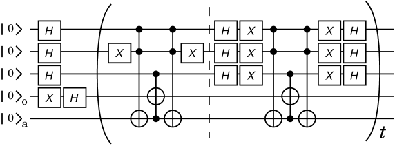
Figure 2: Quantum circuit of the three-qubit quantum search described in the text. The circuit in the parentheses illustrates $R$, in which the left half corresponds to $(1-2|101\rangle\langle 101|)$ and the right half corresponds to $(1-2|s\rangle\langle s|)$. Symbol “o” stands for the oracle qubit and “a” stands for the ancilla qubit.

In addition, here, truncations of nonzero Schmidt coefficients were not employed.

We plot the computational error $|\widetilde{\rm Prob}_{101}(20)-{\rm Prob}_{101}(20)|$ after 20 iterations of the Grover routine against the precision in figure 3, where $\widetilde{\rm Prob}_{101}(20)$ is a computed value and ${\rm Prob}_{101}(20)=|\langle 101|R^{20}|s\rangle|^{2}=\frac{5327874951961}{8796093022208}$ is the exact value calculated symbolically by the Maxima system [26] with the Qcomp.mac package [27].

Figure 3: Computational error $|\widetilde{\rm Prob}_{101}(20)-{\rm Prob}_{101}(20)|$ plotted against the precision.

It is manifest that the double precision (53 bits) is not enough and more than 70 bits precision is preferable for an accurate simulation. In addition, it is interesting that the computational error does not look like a simple elementary function of the precision; there is a sudden drop at a certain value of the precision.

We next evaluate the computational cost by increasing the precision of the TDMPS simulation. The real CPU time used for simulating the above Grover search is plotted against the precision in figure 4. In the figure, we employed a polynomial for coarse fitting, since the computational cost of a TDMPS simulation of a quantum algorithm is guaranteed to be some polynomial in the floating-point precision $p$ (in bits) because each basic arithmetic operation is performed within polynomial time. It can be exponential in the input size of a problem instance, but this is not of our present interest. One might expect that the cost grows quasi-linearly in $p$ considering the cost of each floating-point multiplication. However, the value of $p$ does effect on the number of inverse iterations to guarantee enough accuracy in each matrix diagonalization. In this sense, the fitting seems plausible.

Figure 4: Computation time to simulate 20 iterations of the Grover routine, plotted against the precision. The average was taken over 10 trials for each data point. Error bars span from the minimum to the maximum. Here, $f(p)=1.5\times 10^{-9}(p-64)^{3}+1.0\times 10^{-5}(p-64)^{2}+3.0$. Environment: Redhat Enterprise Linux 6 on Intel Xeon X7542 CPU 2.67GHz, 132GB memory.

The maximum Schmidt rank of the MPS at the time steps between basic quantum gates was $4$ during the above simulation. One may find it smaller than expected. This is because operations $\in{\rm U}(8)$ are simulated without decomposition in terms of ${\rm U}(4)$ and ${\rm U}(2)$ operations, in ZKCM_QC.

3.1.2 Example 2

The sudden drop of the numerical error found in figure 3 is not specific to the example. We will now find a similar behavior in another example. Here, we consider an $n$-qubit quantum circuit shown in figure 5. A Bell state $|\phi\rangle_{0,n-1}=(|0\rangle_{0}|0\rangle_{n-1}+|1\rangle_{0}|1\rangle_{n-1})/\sqrt{2}$ of qubits $0$ and $n-1$ is initially created and then the state $|\phi\rangle_{0,n-1}|0\cdots 0\rangle_{1,\ldots,n-2}$ goes through the quantum Fourier transform (QFT) and its inverse. Thus, the resultant state of the qubits $0$ and $n-1$ should be the initial Bell state. Here, we employ Fowler et al.’s linear-nearest-neighbour construction for QFT [28] exactly as it is.

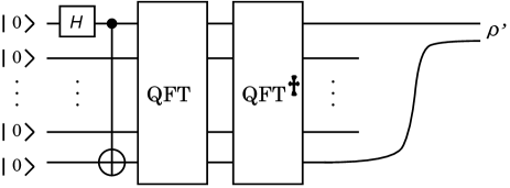
Figure 5: Quantum circuit with QFT and its inverse (${\rm QFT}^{\dagger}$). This circuit has no practical meaning but to examine a numerical error caused by precision shortage in a TDMPS simulation.

Figure 6: Precision dependence of the numerical error $|\langle 00|\widetilde{\rho^{\prime}}|11\rangle-1/2|$ for the three values of $n$.

We performed TDMPS simulations of the circuit for $n=8$, $14$, and $20$ and examined the precision dependence of the numerical error in the $|00\rangle\langle 11|$ element of the reduced density matrix $\rho^{\prime}$ of the qubits $0$ and $n-1$ in the resultant state. Truncations of nonzero Schmidt coefficients were not employed. Ideally, we should have $\langle 00|\rho^{\prime}|11\rangle=1/2$. Let $\widetilde{\rho^{\prime}}$ be the computed matrix; the numerical error is quantified as $|\langle 00|\widetilde{\rho^{\prime}}|11\rangle-1/2|$. We found that the sudden drop of the error appeared for all of the three values of $n$ as shown in figure 6 (Note that the vertical axis is in the logarithmic scale). The figure also indicates that the precision required for avoiding an obvious numerical error tends to grow as the system size grows.

So far we have seen two examples, which have clarified the importance of high-precision computation for accurate TDMPS simulations of quantum computing. We will next examine the truncation error of TDMPS.

3.2 Errors due to truncations

It is uncommon to make use of a truncation of nonzero Schmidt coefficients in TDMPS simulations of quantum computing unlike those used for condensed matter physics as we mentioned in section 1. We however investigate the case we dare to impose truncations. Let us denote the limit on the number of Schmidt coefficients that can be kept for each splitting as $m_{\rm trunc}$. Thus, among Schmidt coefficients, larger $m_{\rm trunc}$ coefficients are kept and the remaining small coefficients are truncated out at each step in the simulation of a quantum circuit.

Here we study the effect of a truncation in a TDMPS simulation of the Deutsch-Jozsa algorithm [24] for a function $f:\{0,1\}^{9}\rightarrow\{0,1\}$ with a nine-bit input ${\bf x}$. Recall that $f$ is either balanced (i.e., $\mathit{\sharp}\{{\bf x}|f({\bf x})=0\}=\mathit{\sharp}\{{\bf x}|f({\bf x})=1\}$) or constant (i.e., $f({\bf x})$ is same for all ${\bf x}$) by the promise of the problem definition for the algorithm (see, e.g., section 3.1.2 of [30]). The Deutsch-Jozsa algorithm for nine qubits is interpreted as the following process. (i) Apply $H^{\otimes 9}V_{f}H^{\otimes 9}$ to $|0_{0}\ldots 0_{8}\rangle$ (here, $V_{f}$ is an operation to put the factor $(-1)^{f({\bf x})}$ to the states $|{\bf x}\rangle$); (ii) Measure the nine qubits of the resultant state. When $f$ is balanced, the probability of having the nine qubits in $|0\rangle$’s simultaneously in the resultant state vanishes; when $f$ is constant, the probability is exactly unity.

We employ the following function for our TDMPS simulation. $f({\bf x})=g(x_{0}x_{1}x_{2})\oplus g(x_{3}x_{4}x_{5})\oplus g(x_{6}x_{7}x_{8})$ with $g({\bf y})=[(\neg y_{0})\wedge(\neg y_{1})]\vee(y_{1}\wedge y_{2})$. This function is balanced. In addition, more specifically, we have ${\rm Prob}(0_{0}0_{1}0_{2})=0$ in the resultant state of (i) for this particular function. The quantum circuit of the Deutsch-Jozsa algorithm for this function is illustrated in figure 7.

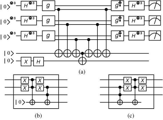
Figure 7: Quantum circuit of the Deutsch-Jozsa algorithm for the function $f$. Circuits (b) and (c) describe the gates $g$ and $g^{\dagger}$ of circuit (a), respectively.

We set the floating-point precision to 256 bits and tried several different values of $m_{\rm trunc}$ in the TDMPS simulation of the quantum circuit. As shown in figure 8, the error in the computed value of ${\rm Prob}(0_{0}0_{1}0_{2})$ (namely, a discrepancy from zero in the present context) vanishes for $m_{\rm trunc}\geq 12$ while a considerable error exists for $m_{\rm trunc}\leq 11$. The largest value among $m_{s}$’s during the simulation is shown as $m_{\rm max}$ in the figure. It indicates that $m_{\rm trunc}$ should be set to at least the maximum possible value of $m_{\rm max}$ which is $12$ in the present case, so as to avoid a nonnegligible error.

Figure 8: Plot of the error in the computed value of ${\rm Prob}(0_{0}0_{1}0_{2})$ (crosses) and the plot of $m_{\rm max}$ (boxes) as functions of $m_{\rm trunc}$. See the text for the details of the simulation.

The above result shows that we cannot truncate out any nonzero Schmidt coefficient during the simulation. This phenomenon should be related to the distribution of Schmidt coefficients if discussions of reference [9] apply to the present case. We show the distribution at the points we had the maximum Schmidt rank $12$ in the simulation, in figure 9 (this is same for both of the points). These points were the second CNOT gate from the left and one from the right among the seven CNOT gates in the middle part of circuit (a) of figure 7. It is now manifest that none of the twelve Schmidt coefficients is negligible. This is how even a single truncation caused a significant error.

Figure 9: Distribution of Schmidt coefficients for the splitting at the points we had the maximum Schmidt rank in the simulation. The distribution was same for both of the points.

4 Discussion

The TDMPS method is regarded as an approximation method in condensed matter physics, but is usually an exact method in simulation studies of quantum computing. Truncations of nonzero small Schmidt coefficients are thus unemployed, usually, for the purpose of simulating quantum computation. In a known case in condensed matter physics [9] where we should avoid truncations, a dominant number of Schmidt coefficients are nonnegligible. This should be true also in TDMPS simulations of quantum circuits. In fact, we found that this is the case and the threshold $m_{\rm trunc}$ for the largest number of surviving Schmidt coefficients should be at least the maximum possible number of nonzero Schmidt coefficients, in the simulation results for the Deutsch-Jozsa algorithm presented in section 3.2.

Besides, we have also evaluated the effect of precision shortage. Rounding errors of individual basic arithmetic operations may accumulate to a large error in the resultant state of a TDMPS simulation of a quantum circuit. In our simulation of a simple quantum search presented in section 3.1.1, a nonnegligible error was observed in the resultant population of a target state unless we increased the precision beyond the double precision. Furthermore, we found that the error does not behave like a smooth curve as a function of the precision in bits, but behaves like a step function with a sudden drop, as shown in figure 3. This phenomenon was also observed in the TDMPS simulation of a quantum circuit containing the quantum Fourier transform, for three different system sizes, as presented in section 3.1.2. In addition, this is not a particular phenomenon for a TDMPS simulation but a rather commonly observed one for matrix computation (see the document of the ZKCM library [19]).

With our simulation results for investigating numerical errors, it is suggested that the precision should be preferably at least 70 bits and the truncation of nonzero Schmidt coefficients is not encouraged for a TDMPS simulation of quantum computation. As for the cost of multiprecision computation, figure 4 indicates that more than 1000 bits precision is quite expensive. As a matter of fact, the current computer architecture does not have a good hardware support for high precision computation. Thus the practical precision we may employ should be several hundreds bits for the time being.

5 Conclusion

We have utilized our multiprecision TDMPS library ZKCM_QC to investigate numerical errors in TDMPS simulations of quantum computing. To avoid a nonnegligible rounding error within a practical cost, it is suggested that the length of the mantissa portion of each floating-point number should be beyond the double-precision length but not more than 1000 bits in the present technology. It is also suggested that a truncation of nonzero Schmidt coefficients is discouraged.

6 Software information

The simulations were performed with ZKCM_QC ver. 0.0.9beta put on the repository
https://sourceforge.net/p/zkcm/sublibqc .

References

References

- [1] White S R 1993 Phys. Rev. B 48 10345
- [2] Schollwöck U 2005 Rev. Mod. Phys. 77 259–315
- [3] Schollwöck U 2011 Ann. Phys. 326 96–192
- [4] SaiToh A ZKCM_QC https://sourceforge.net/p/zkcm/home/Extension Packages/; see also Preprint arXiv:1111.3124
- [5] Vidal G 2003 Phys. Rev. Lett. 91 147902
- [6] SaiToh A and Kitagawa M 2006 Phys. Rev. A 73 062332
- [7] Bauer B et al. 2011 J. Stat. Mech. 2011(05) P05001; http://alps.comp-phys.org/
- [8] Bailey D H, Barrio R and Borwein J M 2012 Appl. Math. Comput. 218 10106–10121
- [9] Venzl H, Daley A J, Mintert F and Buchleitner A 2009 Phys. Rev. E 79 056223
- [10] Bañuls M C, Orús R, Latorre J I, Pérez A and Ruiz-Femenía P 2006 Phys. Rev. A 73 022344
- [11] Kawaguchi A, Shimizu K, Tokura Y and Imoto N Classical simulation of quantum algorithms using the tensor product representation Preprint arXiv:quant-ph/0411205
- [12] Markov I L and Shi Y 2008 SIAM J. Comput. 38 963–981
- [13] Yoran N and Short A J 2006 Phys. Rev. Lett. 96 170503
- [14] Jozsa R On the simulation of quantum circuits Preprint arXiv:quant-ph/0603163
- [15] Chamon C and Mucciolo E R 2012 Phys. Rev. Lett. 109 030503
- [16] Temme K and Wocjan P Efficient computation of the permanent of block factorizable matrices Preprint arXiv:1208.6589
- [17] Johnson T H, Biamonte J D, Clark S R and Jaksch D 2013 Sci. Rep. 3 1235
- [18] Hallberg K A 2006 Adv. Phys. 55 477–526
- [19] Documents linked from http://zkcm.sf.net/
- [20] The GNU multiple precision arithmetic library http://gmplib.org/
- [21] Fousse L, Hanrot G, Lefèvre V, Pélissier P and Zimmermann P 2007 ACM Trans. Math. Software 33 13; http://www.mpfr.org/
- [22] Grover L K 1996 Proceedings of the 28th Annual ACM Symposium on Theory of Computing (STOC 1996) (Philadelphia, PA: ACM Press, New York, 1996) pp 212–219
- [23] Shor P W 1997 SIAM J. Comput. 26 1484–1509
- [24] Deutsch D and Jozsa R 1992 Proc. Royal Soc. London A 439 553–558
- [25] Garey M R and Johnson D S 1979 Computers and Intractability: A Guide to the Theory of NP-Completeness (New York: W.H. Freeman and Co.)
- [26] Maxima, a computer algebra system http://maxima.sourceforge.net/
- [27] SaiToh A Qcomp.mac http://silqcs.org/∼saitoh/qcomp.mac
- [28] Fowler A G, Devitt S J and Hollenberg L C L 2004 Quant. Inf. Comput. 4 237–251
- [29] Draper T G Addition on a quantum computer Preprint arXiv:quant-ph/0008033
- [30] Gruska J 1999 Quantum Computing (Berkshire, UK: McGraw-Hill)