Pebbling in Split Graphs
 

Abstract

Graph pebbling is a network optimization model for transporting discrete resources that are consumed in transit: the movement of two pebbles across an edge consumes one of the pebbles. The pebbling number of a graph is the fewest number of pebbles $t$ so that, from any initial configuration of $t$ pebbles on its vertices, one can place a pebble on any given target vertex via such pebbling steps. It is known that deciding if a given configuration on a particular graph can reach a specified target is NP-complete, even for diameter two graphs, and that deciding if the pebbling number has a prescribed upper bound is $\Pi_{2}^{\sf P}$-complete.

On the other hand, for many families of graphs there are formulas or polynomial algorithms for computing pebbling numbers; for example, complete graphs, products of paths (including cubes), trees, cycles, diameter two graphs, and more. Moreover, graphs having minimum pebbling number are called Class 0, and many authors have studied which graphs are Class 0 and what graph properties guarantee it, with no characterization in sight.

In this paper we investigate an important family of diameter three chordal graphs called split graphs; graphs whose vertex set can be partitioned into a clique and an independent set. We provide a formula for the pebbling number of a split graph, along with an algorithm for calculating it that runs in $O(n^{\beta})$ time, where ${\beta}=2{\omega}/({\omega}+1)\cong 1.41$ and ${\omega}\cong 2.376$ is the exponent of matrix multiplication. Furthermore we determine that all split graphs with minimum degree at least 3 are Class 0.

Key words. pebbling number, split graphs, Class 0, graph algorithms, complexity

MSC. 05C85 (68Q17, 90C35)

1 Introduction

Graph pebbling is a network optimization model for transporting discrete resources that are consumed in transit: while two pebbles cross an edge of a graph, only one arrives at the other end as the other is consumed (or lost to a toll, one can imagine). This operation is called a pebbling step. The basic questions in the subject revolve around deciding if a particular configuration of pebbles on the vertices of a graph can reach a given root vertex via pebbling steps (for this reason, graph pebbling is carried out on connected graphs only). If a configuration can reach $r$, it is called $r$-solvable, and $r$-unsolvable otherwise.

Various rules for pebbling steps have been studied for years and have found applications in a wide array of areas. One version, dubbed black and white pebbling, was applied to computational complexity theory in studying time-space tradeoffs (see [15, 28]), as well as to optimal register allocation for compilers (see [30]). Connections have been made also to pursuit and evasion games and graph searching (see [21, 27]). Another (black pebbling) is used to reorder large sparse matrices to minimize in-core storage during an out-of-core Cholesky factorization scheme (see [12, 22, 24]). A third version yields results in computational geometry in the rigidity of graphs, matroids, and other structures (see [13, 31]). The rule we study here originally produced results in combinatorial number theory and combinatorial group theory (the existence of zero sum subsequences — see [4, 11]) and have recently been applied to finding solutions in $p$-adic diophantine equations (see [23]). Most of these rules give rise to computationally difficult problems, which we discuss for our case below.

We follow fairly standard graph terminology (e.g. [32]), with a graph $G=(V,E)$ having $n=n(G)$ vertices $V=V(G)$ and having edges $E=E(G)$. The eccentricity ${\sf ecc}(G,r)$ for a vertex $r\in V$ equals $\max_{v\in V}{\sf dist}(v,r)$, where ${\sf dist}(x,y)$ denotes the length (number of edges) of the shortest path from $x$ to $y$; the diameter ${\sf diam}(G)=\max_{r\in V}{\sf ecc}(G,r)$. When $G$ is understood we will shorten our notation to ${\sf ecc}(r)$.

The most studied graph pebbling parameter, and the one investigated here, is the pebbling number $\pi(G)=\max_{r\in V}\pi(G,r)$, where $\pi(G,r)$ is defined to be the minimum number $t$ so that every configuration of size at least $t$ is $r$-solvable. The size $|C|$ of a configuration $C:V{\rightarrow}{\mathbb{N}}=\{0,1,\ldots\}$ is its total number of pebbles $\sum_{v\in V}C(v)$. Simple lower bounds like $\pi(G)\geq n$ (sharp for complete graphs, cubes, and, probabilisticaly, almost all graphs) and $\pi(G)\geq 2^{{\sf diam}(G)}$ (sharp for paths and cubes, among others) are easily derived. Graphs satisfying $\pi(G)=n$ are called Class $0$ and are a topic of much interest (e.g. [2, 3, 5, 6, 9, 10]). Surveys on the topic can be found in [16, 17, 19], and include variations on the theme such as $k$-pebbling, fractional pebbling, optimal pebbling, cover pebbling, and pebbling thresholds, as well as applications to combinatorial number theory and combinatorial group theory (see references).

Computing graph pebbling numbers is difficult in general. The problem of deciding if a given configuration of pebbles on a graph can reach a particular vertex was shown in [14, 20] to be NP-complete (via reduction from the problem of finding a perfect matching in a $4$-uniform hypergraph). The problem of deciding if a graph $G$ has pebbling number at most $k$ was shown in [14] to be $\Pi_{2}^{\sf P}$-complete.

On the other hand, pebbling numbers of many graphs are known: for example, cliques, trees, cycles, cubes, diameter two graphs, graphs of connectivity exponential in its diameter, and others. In particular, in [26] the pebbling number of a diameter $2$ graph $G$ was determined to be $n$ or $n+1$. Moreover, [5] characterized those graphs having $\pi(G)=n+1$ (a slight error in the characterization was corrected by [3]). All such connectivity $1$ graphs have $\pi(G)=n+1$. The smallest such $2$-connected graph is the near-Pyramid on $6$ vertices, which is the $6$-cycle $(r,a,p,c,q,b)$ with an extra two or three of the edges of the triangle $(a,b,c)$ (the Pyramid has all three). All diameter $2$ graphs with pebbling number $n+1$ can be described by adding simple structures to the near-Pyramid. It was shown in [14] that one can recognize such graphs in quartic time.

Here we begin to study for which graphs their pebbling numbers can be calculated in polynomial time. Aiming for tree-like structures (as was considered in [6]), one might consider chordal graphs of various sorts. Moving away from diameter $2$, one might consider diameter $3$ graphs; recently ([29]), the tight upper bound of ${\lfloor}3n/2{\rfloor}+2$ has been shown for this class. Combining these two thoughts we study split graphs in this paper, and find that their pebbling numbers can be calculated quickly, in fact, in $O(n^{1.41})$ time.

Split graphs can be described by adding simplicial vertices (cones) to a fixed clique. In other words, a graph is a split graph if its vertices can be partitioned into an independent set $S$ and a clique $K$. Notice that the Pyramid is a split graph with clique $\{a,b,c\}$ and cone vertices $r$, $p$, and $q$. The Pyramid plays a key role in the theory of split graphs. However, the Pyramid has diameter $2$, and we are interested in diameter $3$ split graphs.

It turns out that Pereyra and Phoenix graphs (which we define below and necessarily contain the Pyramid) are important for our work (see Fig. 1). We say that $G$ has a Pyramid if there exist three cone vertices with degree $2$ whose neighborhoods do not have the Helly property (that is, their neighborhoods form a triangle). We say that the subgraph induced by the closed neighborhoods of the three cone vertices is a Pyramid of $G$. If $r$ is one of the three cone vertices we say it is an $r$-Pyramid. A graph $G$ is called $r$-Pereyra if it has an $r$-Pyramid, none of whose vertices is a cut vertex of $G$. Denote by ${{\delta}^{*}}(G,r)$ the minimum degree among all vertices at maximum distance from $r$. A graph $G$ is $r$-Phoenix if it is $r$-Pereyra, ${\sf ecc}(r)=3$, and ${{\delta}^{*}}(G,r)\geq 4$. A Pereyra (resp. Phoenix) graph is $r$-Pereyra (resp. $r$-Phoenix) for some $r$.

   

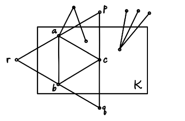
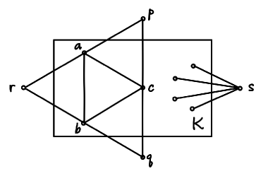
Figure 1: Examples of Pereyra (left) and Phoenix (right) graphs

Like the Pyramid, an $r$-Pereyra graph having ${\sf ecc}(r)=2$ has pebbling number one more than “normal”; that is, it is an exception to how most of the graphs in its class behave. On such $G$, the configuration that places $3$ pebbles on $p$ and $q$, $0$ pebbles on $r$, $a$, $b$, and $c$, and $1$ everywhere else is $r$-unsolvable, showing that $\pi(G,r)\geq n+{\rm x}+1$, where ${\rm x}$ is the number of cut vertices of $G$. (In the course of proving Theorem 3 below, one finds that this configuration is the unique $r$-unsolvable configuration of size $n+{\rm x}$ on $G$.) We will find analogous behavior for $r$-Phoenix graphs as well.

Notationally, we abbreviate ${\sf deg}(x)$ by $d_{x}$. We also abbreviate $N(x)$ by $N_{x}$ (so that $d_{x}=|N_{x}|$), with $[N_{x}]$ denoting $N_{x}\cup\{x\}$. If $v\in S$, we define $K_{v}=K-N_{v}$. We denote the set of cut vertices of $G$ by $X$, with ${\rm x}=|X|$. For a set $U$ of vertices, we write $C(U)=\sum_{x\in U}C(x)$, and define $U^{i}=\{u\in U\mid C(u)=i\}$. For a list of vertices, we denote $C(x_{1},\ldots,x_{k})=(C(x_{1}),\ldots,C(x_{k}))$. We say that a graph is $r$-(semi)greedy if every configuration of size at least $\pi(G,r)$ has a (semi)greedy $r$-solution; that is, every pebbling step in the solution decreases (doesn’t increase) the distance of the moved pebble to $r$. Note that any step from a cone vertex to one of its neighbors is semigreedy.

We begin by outlining in Section 2 a rather new technique for finding upper bounds on $\pi$ using weight functions. From there we prove pebbling number results in the case that ${\sf ecc}(r)=2$. We prepare in Section 4 preliminary lemmas that will be used in Section 5 to prove pebbling results for the ${\sf ecc}(r)=3$ case. In Section 6 we collect recognition results for Pereyra and Phoenix graphs that are combined with our pebbling number theorems to prove our main result that pebbling numbers for split graphs can be calculated in polynomial time. From this analysis we learn that all split graphs with minimum degree at least 3 are Class 0. We end with some comments and conjectures in Section 7.

2 The Weight Function Lemma

In this section we describe a tool developed in [18] for calculating upper bounds for pebbling numbers of graphs that will be useful in delivering a quick proof of Theorem 2.

Let $G$ be a graph and $T$ be a subtree of $G$, with at least two vertices, rooted at vertex $r$. For a vertex $v\in V(T)$ let $v^{+}$ denote the parent of $v$; i.e. the $T$-neighbor of $v$ that is one edge closer to $r$ (we also say that $v$ is a child of $v^{+}$). We call $T$ a strategy when we associate with it a nonnegative, nonzero weight function ${\sf w}:V(T){\rightarrow}{\mathbb{N}}$ with the property that ${\sf w}(r)=0$ and ${\sf w}(v^{+})\geq 2{\sf w}(v)$ for every other vertex that is not a neighbor of $r$ (and ${\sf w}(v)=0$ for vertices not in $T$). We extend ${\sf w}$ to a function on configurations by defining ${\sf w}(C)=\sum_{v\in V}{\sf w}(v)C(v)$. Now denote by ${\mathbf{T}}$ the configuration with ${\mathbf{T}}(r)=0$, ${\mathbf{T}}(v)=1$ for all $v\in V(T)$, and ${\mathbf{T}}(v)=0$ everywhere else. The following was proven in [18].

Lemma 1

[Weight Function Lemma] Let $T$ be a strategy of $G$ rooted at $r$, with associated weight function ${\sf w}$. Suppose that $C$ is an $r$-unsolvable configuration of pebbles on $V(G)$. Then ${\sf w}(C)\leq{\sf w}({\mathbf{T}})$.

The manner in which one uses this lemma to obtain a pebbling number upper bound is as follows. If we have several strategies $T_{1},\ldots,T_{m}$ of $G$, each rooted at $r$, with associated weight functions ${\sf w}_{1},\ldots,{\sf w}_{m}$ and configurations ${\mathbf{T}}_{1},\ldots,{\mathbf{T}}_{m}$, then we can define the accumulated weight function ${\sf w}=\sum_{i=1}^{m}{\sf w}_{i}$ and the accumulated configuration ${\mathbf{T}}=\sum_{i=1}^{m}{\mathbf{T}}_{i}$, and have that ${\sf w}(C)\leq{\sf w}({\mathbf{T}})$ for every $r$-unsolvable configuration $C$. Moreover, if it so happens that ${\sf w}(v)\geq 1$ for all $v\in V-\{r\}$, then we also have $|C|\leq{\sf w}(C)$, from which follows $\pi(G,r)\leq\lfloor{\sf w}({\mathbf{T}})+1\rfloor$.

3 Eccentricity Two

For a split graph $G$ define $X^{r}=X-\{r\}$, with ${{\rm x}^{r}}=|X^{r}|$.

Theorem 2

If $r\in K$ then $G$ is $r$-greedy and $\pi(G,r)=n+{{\rm x}^{r}}$.

Proof.  The lower bound is given by the configuration having $0$ on $r$ and every cut vertex, $3$ on one leaf per vertex in $X^{r}$, and $1$ everywhere else. The upper bound can be proved by using the Weight Function Lemma as follows.

For every neighbor ${r^{\prime}}$ of $r$ we define a strategy $T_{{r^{\prime}}}$. If ${r^{\prime}}\in X$ then give it weight $2$. Include all of its neighbors outside of $K$, giving them weight $1$ each. If ${r^{\prime}}\not\in X$ then give it weight $1$. For every vertex $s$ not yet in some strategy (necessarily not in $K$; also $d_{s}\geq 2$), choose neighbors ${s^{\prime}}$ and $s^{{\prime}{\prime}}$ and include $s$ in both strategies $T_{{s^{\prime}}}$ and $T_{s^{{\prime}{\prime}}}$ with weight $1/2$ each. The resulting sum of strategies has weight $2$ on every vertex in $X^{r}$, and weight $1$ everywhere else. Hence $\pi(G,r)\leq n+{{\rm x}^{r}}$.

Greediness follows because every strategy used is $r$-greedy. $\Box$

We recall the theorem of [3, 5] that if $G$ is a $2$-connected, diameter $2$ graph then $\pi(G)=n+1$ if and only if $G$ is a member of the following special class of graphs ${\cal F}$. First, ${\cal F}$ contains the Pyramid $P$, as well as $P-e$ for any edge $e$ of the triangle $(a,b,c)$. Notice that these graphs have the following separation property: $\{a,b\}$ separates $r$ from $c$, $\{b,c\}$ separates $q$ from $a$, and $\{a,c\}$ separates $p$ from $b$. Next, ${\cal F}$ is closed by adding cones over pairs or triples from $\{a,b,c\}$. Finally, ${\cal F}$ is closed by adding edges between cone vertices, provided that we maintain the separation property. Thus, if $G$ is a $2$-connected split graph of diameter $2$, then $G\in{\cal F}$ if and only if $G$ is Pereyra. In particular, we obtain the diameter $2$ case of Theorem 3, below, when ${\rm x}=0$ (i.e. $G$ is $2$-connected).

For a cone vertex $r$, we have two cases since ${\sf ecc}(r)\in\{2,3\}$. We first note that, in the case ${\sf ecc}(r)=2$, every $r$-unsolvable configuration $C$ has $C(v)\leq 3$ for all $v$. In particular, the solution moving pebbles directly to $r$ from a vertex with $C(v)\geq 4$ is greedy. Recall that ${\rm x}=|X|$.

Theorem 3

If $r$ is a cone vertex with ${\sf ecc}(r)=2$, then $G$ is $r$-semigreedy and $\pi(G,r)=n+{\rm x}+{\psi}$, where ${\psi}={\psi}(G,r)$ is $1$ if $G$ is $r$-Pereyra and $0$ otherwise.

Proof.  The lower bound for non $r$-Pereyra graphs is given by the configuration having $0$ on $r$ and every cut vertex, $3$ on one leaf per cut vertex, and $1$ everywhere else. For $r$-Pereyra graphs we place $0$ on $r$, $a$, $b$, and $c$, $3$ on $p$ and $q$, and $1$ everywhere else ($X={\emptyset}$ because ${\sf ecc}(r)=2$).

We first prove the upper bound directly for $r$-Pereyra graphs. If $G$ is $r$-Pereyra then $N_{r}=\{a,b\}$, and since ${\sf ecc}(r)=2$ we have ${\rm x}=0$ and $[N_{x}]\cap\{a,b\}\neq{\emptyset}$ for all $x$. If $C$ is $r$-unsolvable of size $|C|=n+1$ then $C(r)=0$ and some $C(x)\geq 2$ with, say, $a\sim x$. Thus $C(a)=0$, and also $C(y)\leq 1$ for all $y\in N_{a}$. Now we have $n+1$ pebbles on $n-2$ vertices, which means there must be another vertex $z$, with $b\sim z\not\sim a$, having $C(z)\geq 2$, and so $C(b)=0$. This puts the $n+1$ pebbles on just $n-3$ vertices, which can only happen if $C(r,a,b,x,z)=(0,0,0,3,3)$ and $C(y)=1$ for all other $y$. But this allows us to solve $r$ by moving a pebble from $x$ to $a$, from $z$ to a common neighbor of $z$ and $a$ and then to $a$, and finally from $a$ to $r$. This contradiction means that every configuration of size $n+1$ is $r$-solvable.

Next we prove the upper bound for non $r$-Pereyra $G$. The lower bound is given by the following two unsolvable configurations having size $n+{\rm x}-1$. The first, when $r$ is the only leaf, has $0$ on $r$ and its neighbor ${r^{\prime}}$, $3$ on some $x\neq{r^{\prime}}$, and $1$ everywhere else. Otherwise, the second has $0$ on $r$ and every cut vertex, $3$ on one leaf per vertex in $X^{r}$, and $1$ everywhere else.

For the upper bound, as described above, the result is true for diameter $2$ graphs, and so we may assume that ${\sf diam}(G)=3$. This means that $d_{r}\geq 2$ because, otherwise, ${\sf ecc}(r)=2$ would require that every vertex is adjacent to the neighbor of $r$. Moreover, ${\sf diam}(G)=3$ implies that there are at least two cones different from $r$, whose neighborhoods are disjoint. We remark first that, with eccentricity $2$, the only nonsemigreedy move is one from distance $1$ to distance $2$; but if a move from distance $1$ is possible then it can move to $r$ immediately. Therefore every $r$-solution can be converted to one which is semigreedy.

If a cone vertex $v\neq r$ has the property that $G-v$ is $r$-Pereyra, then we say that $v$ is bad; otherwise it is a good cone vertex. Notice that a bad cone vertex is necessarily a leaf adjacent to a neighbor of $r$; in addition, it is the unique such leaf and $d_{r}=2$. Let $C$ be a configuration of size $n+{\rm x}$. We argue by induction (on the number of cone vertices) and contradiction that $C$ is $r$-solvable.

Suppose that $C$ is not $r$-solvable, let $v$ be any cone vertex, and define ${G^{\prime}}=G-v$, with ${C^{\prime}}=C$ on ${G^{\prime}}$ and ${C^{\prime}}(v)=0$. Also define ${{\rm x}^{\prime}}={\rm x}({G^{\prime}})$ and ${\psi^{\prime}}={\psi}({G^{\prime}})$. Because ${C^{\prime}}$ is $r$-unsolvable on ${G^{\prime}}$, we have $n-C(v)+{\rm x}=|{C^{\prime}}|<\pi({G^{\prime}},r)$. By induction, $\pi({G^{\prime}},r)=(n-1)+{{\rm x}^{\prime}}+{\psi^{\prime}}\leq(n-1)+{\rm x}$ whether $v$ is good or bad: if $v$ is good it holds because ${{\rm x}^{\prime}}\leq{\rm x}$ and ${\psi^{\prime}}=0$, and if $v$ is bad it holds because ${{\rm x}^{\prime}}=0$, ${\psi^{\prime}}=1$, and ${\rm x}=1$. Therefore we may assume that $C(v)\geq 2$.

If $C(v)=2$, then move a pebble from $v$ to one of its neighbors to form $C^{*}$. Then $C^{*}$ is a configuration on ${G^{\prime}}$ of size $n-1+{\rm x}$, which by induction is $r$-solvable. On the other hand, if $C(v)\geq 3$, then $C(v)=3$. We can make the above argument for each cone vertex; thus we may assume that $C(v)=3$ for every cone vertex. Hence no neighbor of $r$ is adjacent to more than one cone vertex, and every neighbor of $r$ adjacent to some cone vertex must have no pebble. Furthermore, if some $x\in K$ has two pebbles then we can move pebbles greedily from $v$ to its common neighbor ${r^{\prime}}$ of $r$, from $x$ to ${r^{\prime}}$, and then from ${r^{\prime}}$ to $r$. Hence we may assume that $C(x)\leq 1$ for all $x\in K$.

Recall that there are at least two cone vertices. If $v$ is a cone vertex with neighbor ${v^{\prime}}$ having $C({v^{\prime}})\geq 1$, then move a pebble from another cone vertex $u$ to its common neighbor ${u^{\prime}}$ of $r$. Then move a second pebble from $v$ to ${v^{\prime}}$ to ${u^{\prime}}$ to $r$. Thus we must have $C(N_{v})=0$ for every cone vertex $v$.

We claim that the neighborhoods of cone vertices are pairwise disjoint. Indeed, suppose two cone vertices $u$ and $v$ have a common neighbor $x$. If there is a third cone vertex $w$ (necessarily having $3$ pebbles), then move one to its common neighbor ${w^{\prime}}$ of $r$. Then move pebbles from $u$ and $v$ to $x$, then from $x$ to ${w^{\prime}}$ to $r$. Thus there are no other cone vertices. As mentioned above, if $u$ and $v$ are the only cone vertices then $N_{u}$ and $N_{v}$ are disjoint. This proves the claim.

Now we may partition $G-r$ into closed neighborhoods of cone vertices and one extra part ${K^{\prime}}$ consisting of vertices of $K$ adjacent to no cone. Notice that the above arguments show that $C([N_{v}])=3$ for every cone vertex $v$. Moreover, $3=|[N_{v}]|+1$ when $d_{v}=1$ (i.e. ${v^{\prime}}\in X$), and $3\leq|[N_{v}]|$ otherwise. Also, $C({K^{\prime}})\leq|{K^{\prime}}|$. Hence $|C|\leq n-1+{\rm x}$, a contradiction. $\Box$

We finish this section with a result that will be used to prove Theorem 11 below. Define $\pi_{k}(G,r)$ to be the minimum number of pebbles $t$ so that from every configuration of size $t$ one can move $k$ pebbles to $r$ (such a configuration is called $k$-fold $r$-solvable). For example, $\pi_{1}(G,r)=\pi(G,r)$.

Recall that $X^{r}=X-\{r\}$ and ${{\rm x}^{r}}=|X^{r}|$. Now define ${X_{rs}}=X-N_{r}-N_{s}$, with ${{\rm x}_{rs}}=|{X_{rs}}|$.

Theorem 4

If $r\in K$ and ${\delta}={{\delta}^{*}}(G,r)$ then

$$\pi_{2}(G,r)=\left\{\begin{array}[]{lll}n+{{\rm x}^{r}}+4&\hbox{if}&{\delta}=1;\\ n+6-{\delta}&\hbox{if}&1<{\delta}<4;\\ n+2&\hbox{if}&{\delta}\geq 4.\\ \end{array}\right.$$

Proof.  Suppose ${\delta}=1$. Choose $s$ to be a vertex at distance $2$ from $r$ with $d_{s}={\delta}$, The lower bound is given by the following configuration $C$ of size $n+{{\rm x}^{r}}+3$ that is not $2$-fold $r$-solvable: we place $0$ pebbles on $r$ and each cut vertex, $7$ on $s$, $3$ on one leaf per vertex in ${X_{rs}}$, and $1$ everywhere else. Evidently, the only pebble that can reach $r$ comes from four that are on $s$.

For the upper bound, we assume that $C$ is a configuration of size $n+{{\rm x}^{r}}+4$ that cannot place two pebbles on $r$. If we can place one pebble on $r$ using at most $3$ pebbling steps, then Theorem 2 says we can place another on $r$ with the remaining $n+{{\rm x}^{r}}$ pebbles, so we suppose otherwise.

This means that $C(x)\leq 1$ for all $x\in K$, $C(x)\leq 3$ for all $x$, $C(N_{x})=0$ for all $x\in{S^{+}}=S^{2}\cup S^{3}$, and $N_{x}\cap N_{y}={\emptyset}$ for all $x,y\in{S^{+}}$. Now every $x\in{S^{+}}$ satisfies $|[N_{x}]|+1\geq 3\geq C(x)=C([N_{x}])$, with equality if and only if $x$ is a leaf. Hence, with $L$ denoting the set of leaves, $L^{+}=L\cap{S^{+}}$, and $U=V-\cup_{x\in{S^{+}}}[N_{x}]$, we have

$$|C| =\sum_{x\in L^{+}}C([N_{x}])+\sum_{x\in{S^{+}}-L^{+}}C([N_{x}])+\sum_{x\in U}C(x)$$

$$\leq\sum_{x\in L^{+}}(|[N_{x}]|+1)+\sum_{x\in{S^{+}}-L^{+}}|[N_{x}]|+(|U|-1)$$

$$\leq n+{{\rm x}^{r}}-1,$$

a contradiction.

Now suppose that $1<{\delta}<4$ — notice that ${{\rm x}^{r}}=0$ when ${\delta}>1$. The lower bound comes from the configuration that places $7$ on $s$, $0$ on $r$ and $N_{s}$, and $1$ everywhere else, having size $n+5-{\delta}$. Once again, the only pebble that can reach $r$ comes from four that are on $s$.

The very same upper bound argument above works here when ${\delta}=2$, so we assume that ${\delta}=3$, whereby $C$ has size $n+3$. Suppose $C$ is not $2$-fold $r$-solvable. Then since by Theorem 2 we have $\pi_{1}(G,r)=n$, it must be that:

1. $C(r)=0$,

2. $C(x)\leq 1$ for every $x\in K$,

3. if $x\in S$ and $C(x)\geq 2$ then $C(N_{x})=0$,

4. (by induction) $C(x)\geq 2$ for every $x\in S_{s}$, and

5. if there exists a vertex $x\neq s$ at distance $2$ from $r$ with $d_{x}={\delta}$, then $C(s)\geq 2$.

Now, if there exists $x\in S_{s}$, then by part 4 we have $C(x)\geq 2$, and by part 5 we have $C(N_{x})=0$. Let $h\in N_{x}$, $h\neq r$, and consider ${G^{\prime}}=G-h$. Notice that ${{\delta}^{*}}({G^{\prime}},r)\geq{\delta}-1=2$ so that, by induction, $\pi_{2}({G^{\prime}},r)=n-1+6-{{\delta}^{*}}({G^{\prime}},r)\leq n+3=|C|$. Thus $C$ is $2$-fold $r$-solvable, a contradiction.

Otherwise, $S_{s}=\emptyset$, and we can assume $K=\{r\}\cup N_{s}$. It follows $n=5$, $|C|=8$, and $C$ is $2$-fold $r$-solvable, a contraction.

Finally, suppose that ${\delta}\geq 4$. In this case the lower bound comes from the configuration with $3$ on $s$, $0$ on $r$, and $1$ everywhere else, having size $n+1$. Here, the only pebble that can reach $r$ comes from two on $s$.

For the upper bound, let $C$ be a configuration of size $n+2$ that is not $2$-fold $r$-solvable. Since, by Theorem 2, we have $\pi(G,r)=n$, it must be that $C(r)=0$, and $C(x)\leq 1$ for every $x\in K_{r}$. We will use induction on $|S|$, with the base case of $|S|=1$ (say $S=\{x\}$). In this case we have $C(x)\geq 4$, so $C(N_{x})\leq 1$. Then $C(x)\geq 8-C(N_{x})$, so in either case of $C(N_{x})\in\{0,1\}$ we can put two pebbles on $r$, a contradiction. Now suppose that $|S|\geq 2$.

Let $x\in K_{r}$. Because ${\delta}\geq 4$, $G-x$ is connected and has no cut vertices different from $r$. Denote ${{\delta}^{\prime}}={{\delta}^{*}}(G-x,r)$. Notice that ${{\delta}^{\prime}}\geq{\delta}-1$ and so, by the inductive hypothesis,

$$\pi_{2}(G-x,r)=\left\{\begin{array}[]{ll}n-1+6-3=n+2,&\mbox{ when }{{\delta}^{\prime}}=3;\\ n-1+2=n+1,&\mbox{ when }{{\delta}^{\prime}}\geq 4.\\ \end{array}\right.$$

This implies that if $C(x)=0$ then $C$ is $2$-fold $r$-solvable, a contradiction.

Therefore $C(x)=1$ for every $x\in K_{r}$, thus $C(S)=n+2-|K_{r}|=|S|+3$. This means that in $S$ there is a vertex with at least $4$ pebbles or there are two vertices with at least $2$ pebbles each. In both cases we can place two pebbles on $r$, a contradiction which completes the proof. $\Box$

4 Eccentricity Three

In the case that ${\sf ecc}(r)=3$, define ${D_{3}(r)}$ to be the set of vertices at distance $3$ from $r$, with ${\delta}={{\delta}^{*}}(G,r)$, and let $s\in{D_{3}(r)}$ be chosen to have $d_{s}={\delta}$. Denote by $S$ the set of cone vertices of $G$, with $S_{v}=S-\{v\}$ and ${S_{rs}}=S-\{r,s\}$. Also, let $K_{v}=K-N_{v}$, and ${K_{rs}}=K_{r}-N_{s}$. Recall that ${X_{rs}}=X\cap{K_{rs}}$, with ${{\rm x}_{rs}}=|{X_{rs}}|$. Now let ${X_{0}}$ be the set of cut vertices of $N_{r}$ adjacent to some cone vertex in $S_{r}$, with ${{\rm x}_{0}}=|{X_{0}}|$. Note that ${{\rm x}_{rs}}>0$ implies $d_{s}=1$.

Define the following four functions:

$${t_{rs}}(G,r) =n+{{\rm x}_{rs}}+6-d_{r}-d_{s};$$

$$t_{r}(G,r) =n+{{\rm x}_{rs}}+2-d_{r};$$

$$t_{s}(G,r) =n+{{\rm x}_{rs}}+{{\rm x}_{0}}+2-d_{s};$$

$$t_{0}(G,r) =n+{{\rm x}_{rs}}+{{\rm x}_{0}};$$

and let $t(G,r)=\max\{t_{\alpha}(G,r)\mid{\alpha}\in\{rs,r,s,0\}\}$. Notice that $t$ is well defined: the selection of vertex $s$ does not change the value of $t$. Furthermore, the choice of $S$ in the split representation of $G$ does not influence $t$ either. Also, If $G$ is $r$-Phoenix then $d_{r}=2$, ${{\rm x}_{0}}={{\rm x}_{rs}}=0$, and $d_{s}=4$, which yields $t(G,r)=n$ in this instance.

Next define the following four configurations $C_{\alpha}$ of sizes $|C_{\alpha}|=t_{\alpha}(G,r)-1$.

• $0$ on $r$, $N_{r}$, $N_{s}$, ${X_{rs}}$, $7$ on $s$, $3$ on one leaf per cut vertex in ${X_{rs}}$, and $1$ everywhere else.

• $0$ on $r$, $N_{r}$, and ${X_{rs}}$, $3$ on $s$ and on one leaf per cut vertex in ${X_{rs}}$, and $1$ everywhere else.

• $0$ on $r$, $N_{s}$, ${X_{rs}}$, and ${X_{0}}$, $3$ on $s$ and on one leaf per cut vertex in ${X_{rs}}\cup{X_{0}}$, and $1$ everywhere else.

• $0$ on $r$, ${X_{rs}}$, and ${X_{0}}$, $3$ on one leaf per cut vertex in ${X_{rs}}\cup{X_{0}}$, and $1$ everywhere else.

Also, in the case that $G$ is $r$-Phoenix, define the configuration $C_{P}$ by placing $0$ on $\{r,a,b,c\}$, $3$ on $p$ and $q$, and $1$ everywhere else. Notice that $C_{P}$ witnesses that $\pi(G)\geq n+1$ for every $r$-Phoenix graph $G$.

Lemma 5

Each $C_{\alpha}$ is $r$-unsolvable.

Proof.  For ${\alpha}\in\{s,0\}$ $C_{\alpha}$ is $r$-unsolvable because the only pebbling moves available are from the cones with $3$ pebbles to $K$, and after those no pebbling move is available. In $C_{r}$, the only move available is from $s$ to some $v\in N_{s}$, and then from $v$ along any path to some $u\in N_{r}$, at which point no more moves are available. In ${C_{rs}}$, the leaves with $3$ pebbles can only move to their neighbors, at which point they stop. Then $s$ can only move $3$ to its neighbor, at which point it can travel along any path to some neighbor of $r$ and stop there. Finally, as mentioned in the proof of Theorem 3, $C_{P}$ is $r$-unsolvable on $r$-Pereyra graphs. $\Box$

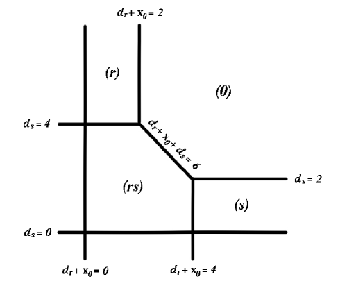
Figure 2: Graph of Cases in Lemma 6

Lemma 6

With the values of $t_{\alpha}$ defined above, we list when (if and only if) each is largest.

• ${t_{rs}}\geq t_{\alpha}$ for all ${\alpha}\in\{s,r,0\}$ when $d_{s}\leq 4$, $d_{r}+{{\rm x}_{0}}\leq 4$, and $d_{r}+d_{s}+{{\rm x}_{0}}\leq 6$;

• $t_{r}\geq t_{\alpha}$ for all ${\alpha}\in\{rs,s,0\}$ when $d_{s}\geq 4$, and $d_{r}+{{\rm x}_{0}}\leq 2$;

• $t_{s}\geq t_{\alpha}$ for all ${\alpha}\in\{rs,r,0\}$ when $d_{r}+{{\rm x}_{0}}\geq 4$, and $d_{s}\leq 2$;

• $t_{0}\geq t_{\alpha}$ for all ${\alpha}\in\{rs,s,r\}$ when $d_{r}+d_{s}+{{\rm x}_{0}}\geq 6$, $d_{r}+{{\rm x}_{0}}\geq 2$, and $d_{s}\geq 2$.

Proof.  Easy to check (see Figure 2). $\Box$

The next lemma shows how the function $t$ changes when some vertex is removed. We say that a vertex $v$ has a false twin if there exists ${v^{\prime}}$ non-adjacent to $v$ such that $N_{v}=N_{{v^{\prime}}}$.

Lemma 7

Let $v\in{S_{rs}}$. Then

1. If $d_{v}\geq 2$ then $t(G-v,r)=t(G,r)-1$.

2. If $d_{v}=1$ and $v$ has at least one false twin different from $r$ then $t(G-v,r)=t(G,r)-1$.

3. If $d_{v}=1$ and $r$ is the only false twin vertex of $v$ then $t(G-v,r)\leq t(G,r)-1$.

4. If $d_{v}=1$, $v$ has no false twins, and $N_{v}{\subseteq}{X_{rs}}$ then $t(G-v,r)=t(G,r)-2$.

5. If $d_{v}=1$, $v$ has no false twins, and $N_{v}{\subseteq}{X_{0}}$ then $t(G-v,r)\leq t(G,r)-1$.

Proof.  This follows from Lemma 6. $\Box$

Corollary 8

If $v\in{S_{rs}}$ then $t(G-v,r)\leq t(G,r)-1$. $\Box$

Lemma 9

If $d_{r}\geq 2$, $x\in N_{r}$ and $N_{x}\cap S=\{r\}$, then $t(G-x,r)\leq t(G,r)$.

Proof.  This follows from Lemma 6. $\Box$

Lemma 10

Let $G$ be non $r$-Phoenix, ${\delta}={{\delta}^{*}}(G,r)$, and assume there exists $v\in S_{r}$ such that ${G^{\prime}}=G-v$ is $r$-Phoenix. Then exactly one of the following statements is true.

1. $v$ is the only vertex of $G$ with degree $1$, and $N_{v}{\subseteq}N_{r}$. In this case, $d_{r}(G)=d_{r}({G^{\prime}})=2$, ${\delta}\geq 4$, ${{\rm x}_{rs}}=0$ and ${{\rm x}_{0}}=1$; thus $t(G,r)=n+1$.

2. ${\delta}\leq 3$ and $v$ is the only vertex of ${D_{3}(r)}$ with $d_{v}={\delta}$. In this case,

   $$t(G,r)=\left\{\begin{array}[]{ll}n+3,&\hbox{\mbox{ if } ${\delta}=1$;}\\ n+4-{\delta},&\hbox{\mbox{ if } $2\leq{\delta}\leq 3$.}\\ \end{array}\right.$$

In both cases, if $w\neq r$ is a cone vertex of an $r$-Pyramid of $G$ then $G-w$ is not $r$-Phoenix and $t(G-w,r)=t(G,r)-1$.

Proof.  This follows from the definition of $r$-Phoenix and from Lemma 6. $\Box$

Theorem 11

If $r$ is a cone vertex with ${\sf ecc}(r)=3$, then $G$ is $r$-semigreedy and $\pi(G,r)=t(G,r)+{\phi}(G,r)$, where ${\phi}(G,r)=1$ if $G$ is $r$-Phoenix and $0$ otherwise.

5 Proof of Theorem 11

The lower bound is given by Lemma 5. The upper bound follows by induction on $n=|V(G)|$. The theorem is trivially true if $n=4$. Suppose that $G$ is a graph with at least $5$ vertices, $r$ a cone vertex with ${\sf ecc}(r)=3$, and $C$ is a configuration on $G$ of size (without loss of generality) exactly $t=t(G,r)+{\phi}(G,r)$. We assume, for the sake of contradiction, that $C$ is not $r$-solvable; in particular, $C(r)=0$. The semigreediness of $G$ will follow from moving pebbles semigreedily to a subgraph that by induction has a resulting semigreedy solution. Among vertices in ${D_{3}(r)}$, let $s$ be chosen to have the minimum degree ${\delta}={{\delta}^{*}}(G,r)$ and, among such, having the maximum number of pebbles.

5.1 $G$ is $r$-Phoenix

Since $G$ is $r$-Phoenix, then $t(G,r)=n$ and so $|C|=n+1$. Let $p\in S$ be a cone vertex of an $r$-Pyramid such that $N_{p}=\{a,c\}$. It is clear that $C(p)\leq 3$. By Lemma 7(1), $t(G-p,r)=t(G,r)-1$. Thus, by the inductive hypothesis, we have $\pi(G-p,r)=t(G-p,r)+{\phi}(G-p,r)=t(G,r)-1+{\phi}(G-p,r)\leq t(G,r)=n$.

If $C(p)\leq 2$, then we can move a pebble from $p$ to $N_{p}$, creating a configuration ${C^{\prime}}$ on $G-p$ of size $n$, which implies that ${C^{\prime}}$, and hence $C$ is $r$-solvable, a contradiction. So we may assume that $C(p)=3$ and, by an analogous argument, that $C(q)=3$ where $q$ is a cone vertex of the $r$-Pyramid such that $N_{q}=\{b,c\}$. Moreover, we can assume that $p$ and $q$ are the only cone vertices with degree $2$ whose neighborhoods are $\{a,c\}$ or $\{b,c\}$. It follows that the graph $G-p$ is not $r$-Phoenix, so ${\phi}(G-p,r)=0$.

Then, as above, we obtain $\pi(G-p,r)=t(G,r)-1+{\phi}(G-p,r)=t(G,r)-1=n-1$. Moving a pebble from $p$ to $N_{p}$, we obtain a configuration ${C^{\prime}}$ on $G-p$ of size $n+1-3+1=n-1$, which implies that ${C^{\prime}}$, and hence $C$ is $r$-solvable, a contradiction.

5.2 $G$ is not $r$-Phoenix

Thus $|C|=t(G,r)+{\phi}(G,r)=t(G,r)+0=t(G,r)$.

5.2.1 $G-v$ is $r$-Phoenix for some $v\in S_{r}$

We consider the two different cases of Lemma 10.

1. The first case of Lemma 10 has $t(G,r)=n+1$ and $v$ at distance $2$ of $r$; thus $C(v)\leq 3$.

   1. If $C(v)\leq 2$, we obtain a configuration ${C^{\prime}}$ of $G-v$ with at least $|C|-1=t(G,r)-1=n$ pebbles. Since $G-v$ is $r$-Phoenix, $t(G-v,r)=n-1$, then, by the inductive hypothesis, $\pi(G-v,r)=t(G-v,r)+{\phi}(G-v,r)=n-1+1=n$. This means that ${C^{\prime}}$, and so $C$, is $r$-solvable, a contradiction.

   2. If $C(v)=3$, let $w\neq r$ be a cone vertex of an $r$-Pyramid, having distance $2$ from $v$. It is clear that $C(w)\leq 1$; thus we obtain a configuration $|{C^{\prime}}|$ of $G-w$ with at least $|C|-1=t(G,r)-1=n$ pebbles. By the observation at the end of Lemma 10, $t(G-w,r)=n+1-1=n$ and $G-w$ is not $r$-Phoenix, then, by the inductive hypothesis, $\pi(G-w,r)=t(G-w,r)+{\phi}(G-w,r)=n+0=n$. This means that ${C^{\prime}}$, and thus $C$, is $r$-solvable, a contradiction.

2. The second case of Lemma 10 has two options for $t(G,r)$, depending on the value of ${\delta}$.

   1. If $d_{v}={\delta}=1$ then $|C|=t(G,r)=n+3$. We can assume that $C(v)\leq 7$.

      1. If $C(v)\leq 6$ then since, by the inductive hypothesis, $\pi(G-v,r)=t(G-v,r)+{\phi}(G-v,r)=n-1+1=n$, it is easy to see that $C$ is $r$-solvable, a contradiction.

      2. If $C(v)=7$ then let $w\neq r$ be a cone vertex of an $r$-Pyramid. It is clear that $C(w)\leq 1$; thus we have a configuration ${C^{\prime}}$ on $G-w$ of size at least $n+2$. By the observation at the end of Lemma 10, $t(G-w,r)=n+3-1=n+2$. Also, $G-w$ is not $r$-Phoenix so, by the inductive hypothesis, $\pi(G-w,r)=t(G-w,r)+{\phi}(G-w,r)=n+2+0=n+2$. This means that ${C^{\prime}}$, and thus $C$, is $r$-solvable, a contradiction.

   2. If $2\leq d_{v}={\delta}\leq 3$, then $|C|=t(G,r)=n+4-d$. Let $p$ be a cone vertex of an $r$-Pyramid such that $N_{p}=\{a,c\}$ with $a\in N_{r}$. Since $G-p$ is not $r$-Phoenix, by Lemma 7 and the inductive hypothesis, we can assume that $C(p)=3$. Thus we find the configuration ${C^{\prime}}$, equal to $C$ on $G-\{w,r\}$, having size $|C|-3=n+4-d-3=n+1-d\geq n-2$. By Theorem 2 we have $\pi(G-\{p,r\},a)=n-2$, and so ${C^{\prime}}$ is $a$-solvable, implying that $C$ is $r$-solvable, a contradiction.

5.2.2 For every $x\in S_{r}$, $G-x$ is not $r$-Phoenix

Recall that $s\in{D_{3}(r)}$ has the maximum number of pebbles among those vertices of ${D_{3}(r)}$ having $d_{s}={\delta}$.

1. Some $v\in{S_{rs}}$ has $C(v)\leq 2$: We obtain a configuration ${C^{\prime}}$ of $G-v$ with at least $|C|-1=t(G,r)-1$ pebbles. By Corollary 8, $t(G-v,r)\leq t(G,r)-1$, so by the inductive hypothesis $\pi(G-v,r)=t(G-v,r)+{\phi}(G-v,r)\leq t(G,r)-1+0=t(G,r)-1$. This means that ${C^{\prime}}$, and hence $C$, is solvable, a contradiction.

2. Some $v\in{S_{rs}}$ has $C(v)\geq 4$ and every other $u\in{S_{rs}}$ has $C(u)\geq 3$: Notice that we can assume that $v\in{D_{3}(r)}$, that $C(x)\leq 3$ for every $x\in{S_{rs}}-\{v\}$, and that $C(y)=0$ and $N_{y}\cap S=\{r\}$ for all $y\in N_{r}$ (in particular, ${{\rm x}_{0}}=0$). Let ${r^{\prime}}\in N_{r}$ and assume that $d_{r}=1$. By Theorem 4 we have

   $$\pi_{2}(G-r,{r^{\prime}})=\left\{\begin{array}[]{lll}n-1+c_{{r^{\prime}}}+4=n+{{\rm x}_{rs}}+4&\hbox{if}&{\delta}=1;\\ n-1+6-{\delta}=n+5-{\delta}&\hbox{if}&1<{\delta}<4;\\ n-1+2=n+1&\hbox{if}&{\delta}\geq 4.\\ \end{array}\right.$$

   By Lemma 6 (since ${{\rm x}_{rs}}=0$ when ${\delta}>1$) we also have

   $$t(G,r)=\left\{\begin{array}[]{lll}n+{{\rm x}_{rs}}-1-1+6=n+{{\rm x}_{rs}}+4&\hbox{if}&{\delta}=1;\\ n-1-{\delta}+6=n+5-{\delta}&\hbox{if}&1<{\delta}<4;\\ n-1+2=n+1&\hbox{if}&{\delta}\geq 4.\\ \end{array}\right.$$

   Thus $C$ can place two pebbles on ${r^{\prime}}$, then one on $r$, a contradiction. It follows that we can assume that $d_{r}\geq 2$, so that the graph $G-{r^{\prime}}$ is connected.

   The configuration ${C^{\prime}}$, the restriction of $C$ to $G-{r^{\prime}}$, has size $|{C^{\prime}}|=|C|=t(G,r)$. By Lemma 9, $t(G-{r^{\prime}},r)\leq t(G,r)$. Since $G-{r^{\prime}}$ is not $r$-Phoenix, we know from the inductive hypothesis that $\pi(G-{r^{\prime}},r)=t(G-{r^{\prime}},r)+{\phi}(G-{r^{\prime}},r)=t(G-{r^{\prime}},r)\leq t(G,r)$. This means that ${C^{\prime}}$, and therefore $C$, is solvable, a contradiction.

3. ${S_{rs}}={\emptyset}$ or every $v\in{S_{rs}}$ has $C(v)=3$:

   1. ${{\rm x}_{0}}\geq 1$: Let $w$ be a leaf adjacent to ${r^{\prime}}\in N_{r}$. By Theorem 2, $\pi(G-r-w,{r^{\prime}})=n-2+{{\rm x}_{rs}}+{\gamma}$ where ${\gamma}=1$ when $d_{s}=1$ and ${\gamma}=0$ otherwise. We move a pebble from $w$ to ${r^{\prime}}$, and consider the configuration ${C^{\prime}}$, the restriction of $C$ to $G-r-w$, of size $t(G,r)-3$. Notice that when $d_{s}=1$ we have $t(G,r)-3\geq t_{s}(G,r)-3=n+{{\rm x}_{rs}}+{{\rm x}_{0}}-ds+2-3=\pi(G-r-w,{r^{\prime}})-{\gamma}+{{\rm x}_{0}}-d_{s}+1\geq\pi(G-r-w,{r^{\prime}})$, and that when $d_{s}>1$ we have $t(G,r)-3\geq t_{0}(G,r)-3=n+{{\rm x}_{rs}}+{{\rm x}_{0}}-3=\pi(G-r-w,{r^{\prime}})-{\gamma}+{{\rm x}_{0}}-1\geq\pi(G-r-w,{r^{\prime}})$. Thus, in both cases, it is possible to move another pebble to ${r^{\prime}}$, a contradiction.

   2. ${{\rm x}_{0}}=0$ and ${{\rm x}_{rs}}\geq 1$: Notice that in this case $C(s)\geq 3$. Let $w$ be a leaf adjacent to ${w^{\prime}}\in{K_{rs}}$.

      1. If $w$ has no false twins, by the inductive hypothesis and by Lemma 7(4), $\pi(G-w,r)=t(G-w,r)=t(G,r)-2$. We move a pebble from $w$ to ${w^{\prime}}$ and consider the configuration ${C^{\prime}}$, the restriction of $C$ to $G-w$ (except with ${C^{\prime}}({w^{\prime}})=C({w^{\prime}})+1$), having size $t(G,r)-3+1=t(G,r)-2=\pi(G-w,r)$. This makes ${C^{\prime}}$, and hence $C$, $r$-solvable, a contradiction.

      2. If $w$ has a false twin, then we can assume that $s$ has no false twins and $C(s)=3$. Thus $w$ can be chosen as $s$ and the proof follows as above.

   3. ${{\rm x}_{0}}=0$ and ${{\rm x}_{rs}}=0$: Recall from Lemma 6 that in this case we have

      $$t(G,r)=\left\{\begin{array}[]{llllll}n-d_{r}-d_{s}+6,&\hbox{if}&d_{r}\leq 4,&d_{s}\leq 4,&d_{r}+d_{s}\leq 6;&(rs)\\ n-d_{r}+2,&\hbox{if}&d_{r}\leq 2,&d_{s}\geq 4;&&(r)\\ n-d_{s}+2,&\hbox{if}&d_{r}\geq 4,&d_{s}\leq 2;&&(s)\\ n,&\hbox{if}&d_{r}\geq 2,&d_{s}\geq 2,&d_{r}+d_{s}\geq 6.&(0)\\ \end{array}\right.$$

      Furthermore, when $d_{r}=1$ we have from Theorem 4 that $|C|=t(G,r)\leq\pi_{2}(G-r,{r^{\prime}})$, where ${r^{\prime}}$ is the neighbor of $r$. Thus we can place two pebbles on ${r^{\prime}}$ and hence solve $r$, a contradiction. So we will assume hereafter that $d_{r}\geq 2$.

      1. $C(N_{r})>0$: Then there exists ${r^{\prime}}\in N_{r}$ with $C({r^{\prime}})=1$. By Theorem 2, $\pi(G-r,{r^{\prime}})=n-1+{\gamma}$, where ${\gamma}=1$ when $d_{s}=1$ and ${\gamma}=0$ otherwise. We consider the configuration ${C^{\prime}}$, the restriction of $C$ to $G-r$ (except with ${C^{\prime}}({r^{\prime}})=0$), having size $t(G,r)-1$, which is at least $\pi(G-r,{r^{\prime}})$ when $d_{s}>1$. When $d_{s}=1$ we see that $t(G,r)-1\geq t_{s}(G,r)-1=n-1+2-1=\pi(G-r,{r^{\prime}})$. In either case, ${C^{\prime}}$ is ${r^{\prime}}$-solvable, a contradiction.

      2. $C(N_{r})=0$: Define the sets

         $${A_{rs}} =\{x\in{S_{rs}}\mid N_{x}\cap N_{r}\neq{\emptyset},N_{x}\cap N_{s}\neq{\emptyset}\},$$

         $$A_{r} =\{x\in{S_{rs}}\mid N_{x}\cap N_{r}\neq{\emptyset},N_{x}\cap N_{s}={\emptyset}\},$$

         $$A_{s} =\{x\in{S_{rs}}\mid N_{x}\cap N_{r}={\emptyset},N_{x}\cap N_{s}\neq{\emptyset}\},{\rm\ and}$$

         $$A_{0} =\{x\in{S_{rs}}\mid N_{x}\cap N_{r}={\emptyset},N_{x}\cap N_{s}={\emptyset}\}.$$

         Of course, $K^{i}={\emptyset}$ for $i\geq 4$. Notice that, whenever $C(s)\geq 4$, $A_{r}\neq{\emptyset}$, ${A_{rs}}\neq{\emptyset}$, $K^{1}\cap N_{r}\neq{\emptyset}$, or some pair of vertices $x,y\in{S_{rs}}$ satisfies $N_{x}\cap N_{y}\neq{\emptyset}$, we can assume both that $K^{i}={\emptyset}$ for $i\geq 2$ and that either $A_{0}={\emptyset}$ or the sets $[N_{x}]$ for $x\in A_{0}$ are pairwise disjoint.

         We will analyze the possible intersections between the neighborhoods of the cone vertices to compare the number of vertices and the size of the configuration. We consider different cases depending on the number of pebbles in $s$. Let ${K^{\prime}}=K-N(S)$.

         1. $6\leq C(s)\leq 7$: In this case $A_{r}={A_{rs}}=A_{s}={\emptyset}$. Thus $n=1+d_{r}+1+d_{s}+\sum_{x\in A_{0}}|[N_{x}]|+|{K^{\prime}}|\geq 1+d_{r}+1+d_{s}+3|A_{0}|+|K^{1}|$. We also have $C(K)=|K^{1}|$, and so $|C|=3|A_{0}|+C(s)+|K^{1}|$. Then $|C|=t(G,r)\geq n-d_{r}-d_{s}+6\geq 1+d_{r}+1+d_{s}+3|A_{0}|+|K^{1}|-d_{r}-d_{s}+6=|C|-C(s)+8$. Thus $C(s)\geq 8$, a contradiction.

         2. $4\leq C(s)\leq 5$: In this case $A_{r}={A_{rs}}={\emptyset}$. Moreover, $K^{1}{\subseteq}N_{s}$, $|A_{s}|+|K^{1}|\leq 1$, and $N_{x}\cap N_{y}={\emptyset}$ for all $\{x,y\}{\subseteq}{S_{rs}}$ ($x\neq y$). This means that $|C|=3|A_{0}|+3|A_{s}|+|K^{1}|+C(s)$ and $n\geq 1+d_{r}+1+d_{s}+\sum_{x\in A_{0}}|[N_{x}]|+|A_{s}|\geq d_{r}+d_{s}+3|A_{0}|+2+|A_{s}|$. Together these imply that $|C|=t(G,r)\geq n-d_{r}-d_{s}+6\geq 3|A_{0}|+8+|A_{s}|=|C|-2|A_{s}|-|K^{1}|-C(s)+8$, and hence $C(s)\geq 8-2|A_{s}|-|K^{1}|\geq 6$, a contradiction.

         3. $2\leq C(s)\leq 3$:

            • If $A_{r}\neq{\emptyset}$: Then ${A_{rs}}=A_{s}={\emptyset}$, $K^{i}={\emptyset}$ for $i\geq 2$, and $K^{1}{\subseteq}N_{A_{r}}-N_{r}-N_{s}$.

              • If $|A_{r}|\leq 2$ then $n\geq 1+d_{r}+1+d_{s}+\sum_{x\in A_{0}}|[N_{x}]|+|A_{r}|+|K^{1}|\geq d_{r}+d_{s}+2+3|A_{0}|+|A_{r}|+|K^{1}|$. Also $3|A_{0}|+3|A_{r}|+C(s)+|K^{1}|=|C|\geq n-d_{r}-d_{s}+6\geq 8+3|A_{0}|+|A_{r}|+|K^{1}|$, which implies the contradiction that $C(s)\geq 8-2|A_{r}|\geq 4$.

              • If $|A_{r}|\geq 3$ then $K^{1}={\emptyset}$ and $n\geq 1+1+d_{s}+\sum_{x\in A_{0}\cup A_{r}}|[N_{x}]|\geq d_{s}+2+3|A_{0}|+3|A_{r}|$. Thus $3|A_{0}|+3|A_{r}|+C(s)=|C|\geq n-d_{s}+2\geq 4+3|A_{0}|+3|A_{r}|$, which implies the contradiction that $C(s)\geq 4$.

            • If $A_{r}={\emptyset}$ and ${A_{rs}}\neq{\emptyset}$: Then ${A_{rs}}$ contains exactly one vertex $w$ and $K^{1}{\subseteq}N_{w}$. In this case we see that the sets $[N_{r}]$, $[N_{x}]$ (for all $x\in A_{0}$), $K^{1}$ and $[N_{s}]$ are pairwise disjoint. Thus $|C|\leq 3+|K^{1}|+3|A_{0}|+C(s)$ and $|C|=t(G,r)\geq n-d_{r}-d_{s}+6\geq 1+d_{r}+1+|K^{1}|+3|A_{0}|+1+d_{s}-d_{r}-d_{s}+6$, which implies $C(s)\geq 6$, a contradiction.

            • If $A_{r}={A_{rs}}={\emptyset}$: Let ${r^{\prime}}\in N_{r}$ and consider ${G^{\prime}}=G-([N_{r}]-{r^{\prime}})$. Notice that if ${\delta}=1$ then $c_{{r^{\prime}}}={{\rm x}_{rs}}+1$, with $c_{{r^{\prime}}}=c_{rs}=0$ otherwise. By Theorem 4,

              $$\pi_{2}({G^{\prime}},{r^{\prime}})=\left\{\begin{array}[]{lll}n-d_{r}+{{\rm x}_{rs}}+5&\hbox{if}&{\delta}=1;\\ n-d_{r}+6-{\delta}&\hbox{if}&1<{\delta}<4\\ n-d_{r}+2&\hbox{if}&{\delta}\geq 4.\\ \end{array}\right.$$

              Since $C(N_{r})=0$, the restriction of $C$ to ${G^{\prime}}$ has size

              $$t(G,r)=\left\{\begin{array}[]{lll}n+{{\rm x}_{rs}}+5-d_{r}&\hbox{if}&{\delta}=1,d_{r}\leq 4;\\ n+{{\rm x}_{rs}}+1&\hbox{if}&{\delta}=1,d_{r}\geq 4;\\ n+4-d_{r}&\hbox{if}&{\delta}=2,d_{r}\leq 4;\\ n&\hbox{if}&{\delta}=2,d_{r}\geq 4;\\ n+3-d_{r}&\hbox{if}&{\delta}=3,d_{r}\leq 3;\\ n&\hbox{if}&{\delta}=3,d_{r}\geq 3;\\ n+1&\hbox{if}&{\delta}\geq 4,d_{r}=1;\\ n&\hbox{if}&{\delta}\geq 4,d_{r}\geq 2.\\ \end{array}\right.$$

              Thus $C$ is $2$-fold ${r^{\prime}}$-solvable, hence $r$-solvable, a contradiction.

         4. $C(s)\leq 1$: In this case, we have a configuration ${C^{\prime}}$ (the restriction of $C$ to $G-s$) of size at least $|C|-1=t(G,r)-1$ on the graph $G-s$. We will show that $\pi(G-s,r)\leq t(G,r)-1$, implying that ${C^{\prime}}$, and hence $C$ is $r$-solvable, a contradiction.

            • If $r$ has eccentricity $2$ in $G-s$ and $G-s$ is not Pereyra: Then $\pi(G-s,r)=n-1$. On the other hand $t(G,r)\geq n$.

            • If $r$ has eccentricity $2$ in $G-s$ and $G-s$ is $r$-Pereyra: Then $\pi(G-s,r)=n-1+1=n$ and $d_{r}=2$. Furthermore, $d_{s}\leq 3$ because $G$ is not $r$-Phoenix. Hence $t(G,r)=n-2-d_{s}+6\geq n+1$.

            • If $r$ has eccentricity $3$ in $G-s$: Then, by the inductive hypothesis, $\pi(G-s,r)=t(G-s,r)$, since we know that $G-s$ is not $r$-Phoenix. Let ${{\delta}^{\prime}}={{\delta}^{*}}(G-s,r)$ and notice that, since any cone vertex of ${S_{rs}}$ has $3$ pebbles and $s$ has just one pebble, then $d_{s}<{{\delta}^{\prime}}$. We have from Lemma 6 that

              $$t(G-s,r)=\left\{\begin{array}[]{lllll}n-d_{r}-{{\delta}^{\prime}}+5&\hbox{if}&d_{r}\leq 4,\ {{\delta}^{\prime}}\leq 4,&&(rs)^{\prime}\\ &&{\rm and\ }d_{r}+{{\delta}^{\prime}}\leq 6;\\ n-d_{r}+1&\hbox{if}&d_{r}\leq 2,\ {{\delta}^{\prime}}\geq 4;&&(r)^{\prime}\\ n-{{\delta}^{\prime}}+1&\hbox{if}&d_{r}\geq 4,\ {{\delta}^{\prime}}\leq 2;&&(s)^{\prime}\\ n-1&\hbox{if}&d_{r}\geq 2,\ {{\delta}^{\prime}}\geq 2,&&(0)^{\prime}\\ &&{\rm and\ }d_{r}+{{\delta}^{\prime}}\geq 6.\end{array}\right.$$

              Observe that the only possible change of cases from $G$ to $G-s$ is from $(rs)$ to $(r)^{\prime}$ or $(0)^{\prime}$, or from $(s)$ to $(0)^{\prime}$. It is easy to see that in all cases, $t(G-s,r)\leq t(G,r)-1$.

This completes the proof. $\Box$

For $n=2m$ ($+1$ if $n$ is odd), define the sun $S_{n}$, to be the split graph with $|K|=m$ and $m$ leaves matched with the vertices of $K$ (and an extra leaf joined to $K$ if necessary). According to Theorem 11 we have $\pi(S_{n})=n+(m-2)+(6-1-1)={\lfloor}3n/2{\rfloor}+2$, showing that the pebbling bound for diameter $3$ graphs given in [29] is tight.

6 Algorithms

We begin with a key construction for finding a Pyramid in a split graph $G$. Suppose that $r$ is a cone vertex of $G$ with $d_{r}=2$. Then let $X$ be the set of cut vertices of $G$, $W$ be the set of degree $2$ vertices of $G$ whose neighbors are in $G-X$ and define the graph $H=H(G)$ to have vertices $\cup_{v\in W}N_{v}$ and edges $\{N_{v}\}_{v\in W}$.

Theorem 12

Given a split graph $G$ and root $r$, recognizing if $G$ is $r$-Pereyra can be done in linear time.

Proof.  Of course $G$ being $r$-Pereyra requires $d_{r}=2$. The graph $H=H(G)$ takes linear time to construct. Then $G$ is $r$-Pereyra if and only if $H$ has a triangle including the edge $N_{r}$, which can be checked in linear time. $\Box$

Corollary 13

Calculating $\pi(G,r)$ when $G$ is a split graph with root $r$ can be done in linear time.

Proof.  The set of cut vertices $X$ of $G$ is the neighborhood of the degree $1$ cone vertices, and so can be calculated in linear time at the start. For $r\in K$, Theorem 2 determines $\pi(G,r)$ immediately. For a cone vertex $r$, we calculate its eccentricity in linear time via breadth-first search. If its eccentricity is $2$ then Theorem 3 determines $\pi(G,r)$ in linear time from recognizing if it is $r$-Pereyra or not. Otherwise, we have ${\sf ecc}(r)=3$. In the breadth-first search we also learned of all cone vertices $s$ at distance $3$ from $r$. As we encounter each such $s$ we keep track of the one having least degree. At the end we calculate $t(G,r)$ immediately from Lemma 6 and find $\pi(G,r)$ via Theorem 11. $\Box$

Finding a triangle in a graph is a well-known problem in combinatorial optimization. The best known algorithm is found in [1], below. Let ${\omega}\cong 2.376$ be the exponent of matrix multiplication, and define ${\beta}=2{\omega}/({\omega}+1)\cong 1.41$.

Algorithm 14

[[1], Theorem 3.5] Deciding whether a graph $G$ with $m$ edges contains a triangle, and finding one if it does, can be done in $O(m^{\beta})$ time.

Theorem 15

Given a split graph $G$, recognizing if it is Pereyra can be done in $O(n^{1.41})$ time.

Proof.  We define $H=H(G)$ as above and see that $G$ is Pereyra if and only if $H$ has a triangle. Then Algorithm 14 decides this in $O(n^{1.41})$ time, since the number of edges of $H$ is at most the number of vertices of $G$. $\Box$

Theorem 16

If $G$ is a diamter 3 split graph then $\pi(G)$ is given as follows.

1. If ${\rm x}\geq 2$ then

   $\pi(G)=n+{\rm x}+2$.

2. If ${\rm x}=1$ then

   $\pi(G)=\left\{\begin{array}[]{ll}n+5-{{\delta}^{*}}&\hbox{if\ }r\hbox{\ is a leaf with\ }{\sf ecc}(r)=3\hbox{\ and\ }{{\delta}^{*}}={{\delta}^{*}}(G,r)\leq 4;\\ n+1&\hbox{otherwise.}\end{array}\right.$

3. If ${\rm x}=0$ then

   $\pi(G)=\left\{\begin{array}[]{ll}n+4-{{\delta}^{*}}&\hbox{if there is a cone vertex\ }r\hbox{\ with\ }d_{r}=2,{\sf ecc}(r)=3\\ &\quad\hbox{and\ }{{\delta}^{*}}={{\delta}^{*}}(G,r)\leq 3;\\ n+1&\hbox{if no such\ }r\hbox{\ exists and\ }G\hbox{\ is Pereyra};\\ n&\hbox{otherwise.}\end{array}\right.$

Proof.  First we remark that ${{\rm x}^{r}}\leq{\rm x}$. Hence we know that $\pi(G)=\pi(G,r)$ for some cone root $r$.

If ${\rm x}\geq 2$ then there exist leaves $r$ and $s$ at distance $3$ from each other (in fact, if $r$ is a leaf then so is $s$). For every such $r$ and $s$ we have $t(G,r)={t_{rs}}(G,r)=n+{{\rm x}_{rs}}+6-d_{r}-d_{s}$ from Lemma 6. Also, ${{\rm x}_{rs}}={\rm x}-2$ and $d_{r}=d_{s}=1$, so that $t(G,r)=n+{\rm x}+2$ when $r$ is a leaf. When ${\sf ecc}(r)=3$ but $r$ is not a leaf, we see that $t(G,r)\leq n+{\rm x}+2$ (with equality if and only if $d_{r}=2$, $d_{s}=1$, and $x_{0}=0$). Finally, when ${\sf ecc}(r)=2$ we have from Theorem 3 that $\pi(G,r)=n+{\rm x}+{\psi}<n+{\rm x}+2$. Hence Theorem 11 implies $\pi(G)=n+{\rm x}+2$.

If ${\rm x}=1$ then $G$ is not Phoenix. When ${\sf ecc}(r)=2$, $G$ is not Pereyra, and so Theorem 3 gives $\pi(G,r)=n+1$. When ${\sf ecc}(r)=3$, the cut vertex $v$ is a neighbor of either $r$ or $s$, and so ${{\rm x}_{rs}}=0$. The function $t_{r}=n+2-d_{r}$ is maximized at $n+1$ when $r$ is a leaf, so $\pi(G)\geq n+1$. Obviously $t_{0}\leq n+1$, and $t_{s}=n+{{\rm x}_{0}}+2-d_{s}\leq n+1$, since $d_{s}=1$ implies ${{\rm x}_{0}}=0$. The function ${t_{rs}}$ is also maximized when $r$ is a leaf. Indeed, if $v\not\in N_{r}$ then $s$ is a leaf. Then with ${r^{\prime}}=s$ having corresponding ${s^{\prime}}\in D_{3}({r^{\prime}})$ we have ${t_{{r^{\prime}}{s^{\prime}}}}\geq{t_{rs}}$ because $d_{r^{\prime}}=d_{s}=1$ and $d_{s^{\prime}}\leq d_{r}$. So we may assume that $v\in N_{r}$. If $r$ is not a leaf then let $w$ be a leaf. But then with ${r^{\prime}}=w$ having corresponding ${s^{\prime}}\in D_{3}({r^{\prime}})$ we have ${t_{{r^{\prime}}{s^{\prime}}}}>{t_{rs}}$ since $d_{r^{\prime}}<d_{r}$ and $d_{s^{\prime}}=d_{s}$. Thus we have $\pi(G)\geq n+5-d_{s}$ when $r$ is a leaf and $s\in D_{3}(r)$ with $d_{s}={{\delta}^{*}}$.

Finally, if ${\rm x}=0$, we note from Lemma 6 and Theorem 11 that the only way to have $\pi(G,r)\geq n+1$ when some cone vertex $r$ has ${\sf ecc}(r)=3$ is either via ${t_{rs}}$ (with $d_{r}=2$ and $d_{s}\leq 3$) or if $G$ is $r$-Phoenix. When a cone vertex $r$ has ${\sf ecc}(r)=2$ then we have $\pi(G,r)=n+1$ if $G$ is $r$-Pereyra, by Theorem 3. Thus $\pi(G,r)=n$ in all other cases.

The above description can be reorganized as follows. Suppose that there is no cone vertex $r$ with $d_{r}=2$ and $s\in D_{3}(r)$ with $d_{s}={{\delta}^{*}}(G,r)\leq 3$. If $G$ is Pereyra then it is $r$-Pereyra for some cone vertex $r$ with $d_{r}=2$. Now we know that either ${\sf ecc}(r)=2$ or ${{\delta}^{*}}(G,r)\geq 4$, the latter case of which makes $G$ $r$-Phoenix. In either case we get $\pi(G,r)=n+1$. $\Box$

Corollary 17

Calculating $\pi(G)$ when $G$ is a split graph can be done in $O(n^{1.41})$ time.

Proof.  Recall that we discover the value of ${\rm x}$ in linear time. So if ${\rm x}\geq 2$ then $\pi(G)=n+{\rm x}+2$. When ${\rm x}=1$ we let $r$ be any leaf of $G$. Using breadth-first search from $r$ we discover if $D_{3}(r)\neq{\emptyset}$ and, if so, find $s\in D_{3}(r)$ with $d_{s}={{\delta}^{*}}(G,r)$. Thus, in linear time we know $\pi(G)$.

Now, if ${\rm x}=0$, we describe a linear algorithm either to find a cone vertex $r$ with $d_{r}=2$ and some $s\in D_{3}(r)$ having $d_{s}\leq 3$ or to conclude that none exist.

For ease of notation, we write $d_{i}$ for $d_{v_{i}}$ and $N_{i}$ for $N_{v_{i}}$. In linear time we can reorder the vertices of $G$ so that $d_{i}=2$ for $1\leq i\leq k$ and $d_{i}=3$ for $k+1\leq i\leq l$. Initialize ${\lambda}(i)$ to be empty for every vertex $v_{i}$ of $G$. Then for each $i\leq k$ we add $i$ to ${\lambda}(j)$ for each $v_{j}\in N_{i}$ and check the size of $L_{i}=\cup_{v_{j}\in N_{i}}{\lambda}(j)$. If $|L_{i}|<i$ then there is some $j<i$ such that $N_{i}\cap N_{j}={\emptyset}$ — choose any $j\in\{1,\ldots,i\}-L_{i}$. In this case we set $r=v_{j}$ and $s=v_{i}$ and quit; otherwise we continue. Then for each $k+1\leq i\leq l$ we only check the size of $L_{i}=\cup_{v_{j}\in N_{i}}{\lambda}(j)$. If $|L_{i}|<k$ then there is some $j\leq k$ such that $N_{i}\cap N_{j}={\emptyset}$ — choose any $j\in\{1,\ldots,k\}-L_{i}$. In this case we set $r=v_{j}$ and $s=v_{i}$ and quit; otherwise we continue. If we have not found $r$ and $s$ by now, they do not exist. This algorithm is linear because of the bounded degrees.

If $r$ and $s$ were found then $\pi(G)=n+6-d_{r}-d_{s}$. If no such $r$ and $s$ exist, we use Theorem 15 to discover if $G$ is Pereyra, which takes $O(n^{1.41})$ time. If it is then $\pi(G)=n+1$, otherwise $\pi(G)=n$. $\Box$

7 Remarks

We begin by noting the following corollary to Theorem 16. Let ${\kappa}(G)$ denote the connectivity of $G$.

Corollary 18

If $G$ is a split graph with ${\delta}(G)\geq 3$ then $G$ is Class 0.

Proof.  The first two instances of the ${\rm x}=0$ case of Theorem 16 require ${\delta}(G)=2$. $\Box$

Note that this implies that every $3$-connected split graph is Class 0. The analogous result with “split” replaced by “diameter two” was proven in [5]. The full characterization of diameter two, connectivity two, non Class 0 graphs in [5] involves the appearance of a Pyramid, whereas for connectivity two, non Class 0 split graphs, Pereyra and Phoenix graphs play a significant role.

With the similarities in structure and function mentioned above between Pyramid and Pereyra graphs, one wonders two things. First, in the diameter $2$ case, it is possible to add edges between twin cone vertices (thus leaving the class of split graphs) without changing the pebbling number; is the same true for diameter $3$? Second, might there be a family of graphs that plays for diameter $4$ graphs the same role played by Pyramid and Pereyra graphs for diameters $2$ and $3$, at least in the case that the root $r$ has eccentricity $2$?

It is interesting that, while one can calculate the pebbling number of a diameter two graph in polynomial time, it was shown in [8] that it is NP-complete to decide if a given configuration on a diameter two graph can solve a fixed root. (The same was proven more recently for planar graphs in [7] — the problem is polynomial for planar diameter two graphs.) In that context we offer the following.

Problem 19

Let $C$ be a configuration on a split graph $G$ with root $r$. Is it possible in polynomial time to determine if $C$ is $r$-solvable?

We also offer the following two conjectures.

Conjecture 20

If $G$ is chordal then $\pi(G)$ can be calculated in polynomial time.

Conjecture 21

For fixed $d$, if ${\sf diam}(G)=d$ then $\pi(G)$ can be calculated in polynomial time.

At the very least we believe that, for a chordal or fixed diameter graph $G$, it can be decided in polynomial time whether or not $G$ is Class $0$.

8 Acknowledgements

The third author thanks the Fulbright International Exchange Program for their support and assistance, the National University of La Plata for their hospitality, the Ferrocarril General Roca for a surprise trip to Pereyra, and his coauthors for their generosidad extraordinaria y mate delicioso.

References

- [1] N. Alon, R. Yuster and U. Zwick, Finding and counting given length cycles, Algorithmica 17 (1997), 209–223.
- [2] A. Bekmetjev and C.A. Cusack, Pebbling algorithms in diameter two graphs, SIAM J. Discrete Math. 22 (2009), 634–646.
- [3] A. Blasiak and J. Schmitt, Degree sum conditions in graph pebbling, Austral. J. Combin. 42 (2008), 83–90.
- [4] F. R. K. Chung, Pebbling in hypercubes, SIAM J. Disc. Math. 2 (1989), 467–472.
- [5] T. Clarke, R. Hochberg and G. Hurlbert, Pebbling in diameter two graphs and products of paths, J. Graph Theory 25 (1997), no. 2, 119–128.
- [6] D. Curtis, T. Hines, G. Hurlbert and T. Moyer, Pebbling graphs by their blocks, Integers: Elec. J. Combin. Number Th. 9 (2009), #G2, 411–422.
- [7] C.A. Cusack, L. Dion and T. Lewis, The complexity of pebbling reachability in planar graphs, preprint.
- [8] C.A. Cusack, T. Lewis, D. Simpson and S. Taggart, The complexity of pebbling in diameter two graphs, SIAM J. Discrete Math. 26 (2012), 919–928.
- [9] A. Czygrinow and G. Hurlbert, Girth, pebbling and grid thresholds, SIAM J. Discrete Math. 20 (2006), 1–10.
- [10] A. Czygrinow, G. Hurlbert, H. Kierstead and W. T. Trotter, A note on graph pebbling, Graphs and Combin. 18 (2002), 219–225.
- [11] S. Elledge and G. Hurlbert, An application of graph pebbling to zero-sum sequences in abelian groups, Integers: Elec. J. Combin. Number Theory 5 (2005), no. 1, #A17, 10pp.
- [12] J. Gilbert, T. Lengauer and R. Tarjan, The pebbling problem is complete in polynomial space, SIAM J. Comput. 9 (1980), 513–525.
- [13] Y. Gurevich and S. Shelah, On finite rigid structures, J. Symbolic Logic 61 (1996), no. 2, 549–562.
- [14] D. Herscovici, B. Hester and G. Hurlbert, -Pebbling and extensions, Graphs and Combin., to appear.
- [15] J. Hopcroft, W. Paul and L. Valiant, On time versus space, J. Assoc. Comput. Mach. 24 (1977), no. 2, 332–337.
- [16] G. Hurlbert, Recent progress in graph pebbling, Graph Theory Notes of New York XLIX (2005), 25–37.
- [17] G. Hurlbert, General graph pebbling, Discrete Appl. Math., in press.
- [18] G. Hurlbert, The weight function lemma for graph pebbling, arXiv:1101.5641 [math.CO] (2011).
- [19] G. Hurlbert, The graph pebbling page, http://mingus.la.asu.edu/hurlbert/ pebbling/pebb.html.
- [20] G. Hurlbert and H. Kierstead, Graph pebbling complexity and fractional pebbling, unpublished (2005).
- [21] L. M. Kirousis and C. H. Papadimitriou, Searching and pebbling, Theoret. Comput. Sci. 47 (1986), no. 2, 205–218.
- [22] Klawe, Maria M., The complexity of pebbling for two classes of graphs. Graph theory with applications to algorithms and computer science (Kalamazoo, Mich., 1984), 475–487, Wiley-Intersci. Publ., Wiley, New York, 1985.
- [23] M. P. Knapp, 2-adic zeros of diagonal forms and distance pebbling of graphs, preprint.
- [24] J. W. H. Liu, An application of generalized tree pebbling to sparse matrix factorization, SIAM J. Algebraic Discrete Methods 8 (1987), no. 3, 375–395.
- [25] K. Milans and B. Clark, The complexity of graph pebbling, SIAM J. Discrete Math. 20 (2006), 769–798.
- [26] L. Pachter, H. Snevily and B. Voxman, On pebbling graphs, Congr. Numer. 107 (1995), 65–80.
- [27] T.D. Parsons, Pursuit-evasion in a graph, in Y. Alani and D. R. Lick, eds., Theory and Applications of Graphs, 426–441, Springer, Berlin, 1976.
- [28] M. S. Paterson and C. E. Hewitt, Comparative schematology, in Proj. MAC Conf. on Concurrent Systems and Parallel Computation, June 2–5, 1970, Woods Hole, Mass., 119–127.
- [29] L. Postle, N. Streib and C. Yerger, Pebbling graphs of diameter 3 and 4, J. Graph Theory, to appear.
- [30] R. Sethi, Complete register allocation problems, SIAM J. Comput. 4 (1975), no. 3, 226–248.
- [31] I. Streinu, L. Theran, Sparse hypergraphs and pebble game algorithms, European J. Combin. 30 (2009), no. 8, 1944–1964.
- [32] D. B. West, Introduction to Graph Theory, Prentice-Hall, Upper Saddle River, NJ (1996).