Accelerated molecular dynamics force evaluation on graphics processing units for thermal conductivity calculations

Abstract

Thermal conductivity is a very important property of a material both for testing theoretical models and for designing better practical devices such as more efficient thermoelectrics, and accurate and efficient calculations of thermal conductivity are very desirable. In this paper, we develop a highly efficient molecular dynamics code fully implemented on graphics processing units for thermal conductivity calculations using the Green-Kubo formula. We compare two different schemes for force evaluation, a previously used thread-scheme, where a single thread is used for one particle and each thread calculates the total force for the corresponding particle, and a new block-scheme, where a whole block is used for one particle and each thread in the block calculates one or several pair forces between the particle associated with the given block and its neighbor particle(s) associated with the given thread. For both schemes, two different classical potentials, namely, the Lennard-Jones potential and the rigid-ion potential are implemented. While the thread-scheme performs a little better for relatively large systems, the block-scheme performs much better for relatively small systems. The relative performance of the block-scheme over the thread-scheme also increases with the increasing of the cutoff radius. We validate the implementation by calculating lattice thermal conductivities of solid argon and lead telluride. The efficiency of our code makes it very promising to study thermal conductivity properties of more complicated materials, especially, materials with interesting nanostructures.

1 Introduction

Recently, graphics processing units (GPU) have attracted more and more attention in the computational physics community due to their large-scale parallelism ability, which has been explored in many kinds of computational physics problems, including gravitational $N$-body simulation [1], classical molecular dynamics simulation [2, 3, 4, 5, 6, 7, 8], classical Monte Carlo simulation [9], quantum Monte Carlo simulation [10], quantum transport [11] and exact diagonalization [12], just to name a few. Despite the achievements obtained so far, the potential of GPU to speed up computational physics applications is far from being fully explored.

One of the physical problems which is very demanding of high performance computing is molecular dynamics (MD) simulation and its GPU acceleration has been studied by several groups [2, 3, 4, 5, 6, 7, 8]. As early as in 2006, Yang et al [2] carried out a proof-of-principle study on the acceleration of equilibrium molecular dynamics simulation for thermal conductivity prediction of solid argon based on the Green-Kubo formula using a GPU. For this purpose, there is no need to update the neighbor list since every particle in the system just oscillates around its equilibrate position. Using a very old GPU, they obtained a speedup of about 10 relative to a single CPU, although their implementation suffers from accuracy loss, which results in a heat current autocorrelation function (HCACF) not decaying to zero but a finite value. After this pioneering work, a few other groups studied the GPU-acceleration of more general MD simulations, mainly oriented to large-scale simulations in biochemical systems, and the problem of neighbor list update attracts special considerations [4, 5, 6, 8]. The reported speedups over CPU implementations range from one to two orders of magnitude, depending on the interaction potential, the simulation size and the cutoff radius used in the simulations.

In this work, we consider the development and optimization of a full GPU implementation of equilibrium MD simulations and use it for thermal conductivity predictions using the Green-Kubo formula. The main difference between our work and the previous ones [3, 4, 5, 6, 7, 8] is that we are more interested in relatively small systems, since size effects for the Green-Kubo method of thermal conductivity prediction are not very significant, and they can often be eliminated with less than several thousand particles. The demand for high performance computing for the Green-Kubo method comes from the fact that the number of simulation steps usually needs to be very large (sometimes as large as $10^{8}$ steps [13]) to ensure a well converged HCACF and the corresponding running thermal conductivity (RTC). Around this simulation size, we find that the conventional approach of force evaluation, where a single thread is assigned to evaluate the total force on one particle [5], can not utilize the computational power of modern GPUs sufficiently. Here, we propose another approach of force evaluation, where one block of threads is assigned to evaluate the total force on one particle, which exhibits significantly superior performance for small-to-intermediate simulation sizes. In the one thread per particle scheme (which will be called the thread-scheme), the number of invoked blocks in the force evaluation kernel, which equals the number of particles divided by the block size, is much smaller than that in the one block per particle scheme (which will be called the block-scheme), where it equals the number of particles. We will demonstrate that the block-scheme can attain its optimal performance for relatively small systems and is several times faster than the thread-scheme for these. Compared with the proof-of-principle study of Yang et al [2], which only calculates the lattice thermal conductivity of solid argon using the simple Lennard-Jones (LJ) potential, we also consider the rigid-ion (RI) potential, which is more computational demanding. On average, two orders of magnitude speedups can be obtained for the evolution part of the MD simulation. For all the tested situations, the acceleration rates for the RI potential are several times larger than those for the LJ potential, reflecting the higher arithmetic intensity for the RI potential. In addition, neighbor list construction and HCACF calculation are also implemented in the GPU and good speedups are obtained for these parts too.

This paper is organized as follows. In Sect. 2, we review the techniques of molecular dynamics simulation for thermal conductivity prediction using the Green-Kubo formula and some important features of CUDA relevant to our implementation. In Sect. 3, we present the detailed algorithms and implementations of our code. In Sect. 4, the performances for the different force evaluation schemes and the different potentials are shown and compared. In Sect. 5, we validate our implementation by computing the lattice thermal conductivities of solid argon and lead telluride at different temperatures. Our conclusions will be presented in Sect. 6.

2 Background

2.1 Green-Kubo method for thermal conductivity calculations

In atomistic calculations of lattice thermal conductivity, both the equilibrium-based and the non-equilibrium-based molecular dynamics simulations can be employed. The non-equilibrium-based method uses the Fourier’s law of heat conduction and is referred to as the direct method. The equilibrium-based method uses the Green-Kubo linear response theory and is referred to as the Green-Kubo method. Schelling et al [14] showed that the equilibrium and the nonequilibrium methods give consistent results. In some cases, the former is more advantageous; in other cases, the reverse is true. The most important advantage of the Green-Kubo method is that it has a much less prominent size effect compared to the direct method. In the direct method, unless the simulation cell is many times longer than the mean-free path, scattering from the heat source and heat sink contributes more to the thermal resistivity than the intrinsic anharmonic phonon-phonon scattering does. In most cases, a value for the thermal conductivity of an infinite system can be reliably obtained by the direct method from simulations of different system sizes and an extrapolation to an infinite system size [14]. However, as pointed out by Sellan et al [15], the linear extrapolation procedure is only accurate when the minimum system size used in the direct method simulations is comparable to the largest mean free paths of the phonons that dominate the thermal transport. As for the computational cost, the Green-Kubo method requires a rather long simulation time ($10^{7}\sim 10^{8}$ time steps) to get a well converged HCACF and thermal conductivity value. To get a well defined temperature gradient, the direct method only requires a relatively short simulation time ($\sim 10^{6}$ time steps). However, the Green-Kubo method is still generally computationally cheaper since one needs to simulate several very large systems when using the direct method to accurately extrapolate to the infinite limit. Additionally, by a single simulation, one can obtain the full thermal conductivity tensor of the system when using the Green-Kubo method, but can only obtain a single component of the thermal conductivity when using the direct method.

According to the Green-Kubo linear response theory [16, 17, 18], the lattice thermal conductivity tensor $\kappa_{\mu\nu}$ can be expressed as a time integral of the HCACF $C_{\mu\nu}(t)$,

$$\kappa_{\mu\nu}=\frac{1}{k_{B}T^{2}V}\int_{0}^{\infty}dtC_{\mu\nu}(t),$$ (1)

where $t$ is the correlation time, $k_{B}$ the Boltzmann’s constant, $V$ the volume and $T$ the temperature. The HCACF $C_{\mu\nu}(t)=\langle J_{\mu}(0)J_{\nu}(t)\rangle$ is computed in the MD simulation by an average over different time origins,

$$C_{\mu\nu}(t)=\frac{1}{M}\sum_{m=0}^{M-1}J_{\mu}(m\delta t)J_{\nu}(m\delta t+t),$$ (2)

where $\delta t$ is the time step and $M$ is the number of time origins to be averaged, which is approximately the number of production steps if the number of correlation steps is much less than the number of production steps. For isotropic 3D materials, the thermal conductivity scalar is usually defined to be the average of the diagonal elements, $(\kappa_{xx}+\kappa_{yy}+\kappa_{zz})/3$. Similarly, for a material isotropic in a plane, the thermal conductivity in that plane can be defined to be $(\kappa_{xx}+\kappa_{yy})/2$. Generally, the Green-Kubo method is able to produce the full tensor of thermal conductivity in a single run. We will use $\mathbf{C}$ to denote the vector with components $C_{xx}$, $C_{yy}$ and $C_{zz}$.

The heat current vector $\mathbf{J}$ (with components $J_{x}$, $J_{y}$ and $J_{z}$) is defined to be the time derivative of the sum of the moments of the site energies of the particles in the system [18],

$$\mathbf{J}=\frac{d}{dt}\sum_{i}^{N}\mathbf{r}_{i}E_{i}=\sum_{i}^{N}\mathbf{v}_{i}E_{i}+\sum_{i}^{N}\mathbf{r}_{i}\frac{d}{dt}E_{i},$$ (3)

where the site energy is the sum of the kinetic energy and the potential energy, $E_{i}=\frac{1}{2}m_{i}\mathbf{v}_{i}^{2}+U_{i}$. For a two-body potential, $U_{i}=\frac{1}{2}\sum_{j}U_{ij}$ and $\mathbf{F}_{i}=\sum_{i}\mathbf{F}_{ij}=\sum_{i}\left(-\frac{\partial}{\partial\mathbf{r}_{i}}\right)U_{ij}$, we have

$$\mathbf{J}=\sum_{i}^{N}\mathbf{J}_{i}=\sum_{i}^{N}\left[\sum_{j\neq i}^{N}\mathbf{J}_{ij}+\left(\frac{1}{2}m_{i}\mathbf{v}_{i}^{2}\right)\mathbf{v}_{i}\right],$$ (4)

where

$$\mathbf{J}_{ij}=\frac{1}{4}\left[\mathbf{v}_{ij}U_{ij}-\mathbf{r}_{ij}\left(\mathbf{F}_{ij}\cdot\mathbf{v}_{ij}\right)\right],$$ (5)

with $\mathbf{r}_{ij}=\mathbf{r}_{j}-\mathbf{r}_{i}$ and $\mathbf{v}_{ij}=\mathbf{v}_{j}+\mathbf{v}_{i}$.

In this paper, we consider two kinds of pair-wise potentials. The first is the LJ potential of the form

$$U_{ij}^{\text{LJ}}=4\epsilon\left(\frac{\sigma^{12}}{r_{ij}^{12}}-\frac{\sigma^{6}}{r_{ij}^{6}}\right),$$ (6)

where $\epsilon$ and $\sigma$ are two parameters of the model, the dimensions of which are [energy] and [length] respectively. For argon, $\epsilon/k_{B}=119.8$ K and $\sigma=3.405$ Å, where $k_{B}$ is the Boltzmann’s constant. This potential has been used by many groups to calculate thermal conductivities of both pure solid argon [19, 20, 21, 22, 23] and argon-krypton composites [24, 25]. The second potential we consider is the RI potential which consists of the Coulomb potential as well as a short range part in the Buckingham form

$$U_{ij}^{\text{Buckingham}}=A_{ij}\exp\left(-\frac{r_{ij}}{\rho_{ij}}\right)-\frac{C_{ij}}{r_{ij}^{6}}.$$ (7)

The presence of the subscripts in the parameters $A_{ij}$, $\rho_{ij}$ and $C_{ij}$ indicates that the values of the parameters depend on the particle types of the interacting pairs.

The other part of the RI potential is the Coulomb potential which is a long range potential, and direct evaluation of it using the traditional Ewald summation is very time consuming for large systems. Instead, the Wolf method [26] is more advantageous both computationally and conceptually. In our work, we use a modified form of the Wolf formula developed by Fennell et al [27], in which both the potential and force are continuous at the cutoff radius,

$$\begin{split}U_{ij}^{\text{Coulomb}}&=\frac{q_{i}q_{j}}{4\pi\epsilon_{0}}\left[\frac{\text{erfc}(\alpha r_{ij})}{r_{ij}}-\frac{\text{erfc}(\alpha R_{c})}{R_{c}}\right.\\ &\left.+\left(\frac{\text{erfc}(\alpha R_{c})}{R_{c}^{2}}+\frac{2\alpha}{\pi^{1/2}}\frac{\exp(-\alpha^{2}R_{c}^{2})}{R_{c}}\right)(r_{ij}-R_{c})\right],\end{split}$$ (8)

where $\alpha$ and $R_{c}$ are the electrostatic damping factor and the cutoff radius, respectively. The RI potential in the Buckingham form is used extensively to study lattice thermal conductivities of various kinds of semiconductors and insulators such as complex silica crystals [28], ZnO [29] and PbTe [30]. In this work, we only consider PbTe, using the potential parameters developed by Qiu et al [31]. Note that in their parameterizations, partial charges are used for both Pb and Te, which are +0.666 and -0.666, respectively.

To obtain the lattice thermal conductivity form HCACF, one usually first fits the HCACF by a double-exponential function [32, 20] with two time parameters and obtains the thermal conductivity by analytical integration of the function. Ideally, the HCACF should decay to zero except for some anomalous systems with divergent thermal conductivity [33]. Therefore, alternatively, one can also directly integrate the HCACF and average the resulting RTC values in an appropriate range of time block [14, 15]. We will show that the RTC will converge to a definite value as long as the simulation time is large enough to obtain a smooth HCACF which decays to zero after a given correlation time.

2.2 Overview of CUDA

In this subsection, we review some techniques for GPU programming with CUDA. We choose to use CUDA as our development tool, although other tools such as OpenCL can be equally used. Only the important features relevant to our implementation are presented here. For a more thorough introduction to CUDA, we refer to the official manual [34]. Although our discussion is based on Tesla M2070, which is of compute capability 2.0, the implementation and optimization can be easily ported to other platforms.

CUDA (Compute Unified Device Architecture) [34] is a parallel computing architecture for a hybrid platform of CPU (the host) and GPU (the device). Our CUDA program consists of both common C/C++ code which is compiled and executed on the host and special functions called kernels invoked from the host and executed on the device. When a kernel is called from the host, a grid of blocks, each of which contains individual threads, are invoked to execute the instructions of the kernel in a single instruction multiple data way. Each individual thread has a unique ID which can be specified by built-in variables such as threadIdx.x and blockIdx.x. The sizes of the grid and the blocks for a kernel are specified at runtime and can also be inferred from built-in variables such as gridDim.x and blockDim.x.

The concept of CUDA is closely connected to the GPU hardware architecture, the knowledge of which is vital for understanding and optimizing CUDA applications. A GPU consists of a number of streaming multiprocessors (SMs) and an SM consists of a number of scalar processors (SPs). For our testing GPU, Tesla M2070, there are 16 SMs and $16\times 32=448$ SPs. The maximum numbers of resident blocks and threads that can be simultaneously invoked within an SM are limited. For GPUs with compute capability 2.x, they are 8 and 1536, respectively [34]. Thus, the theoretically optimal number of threads in a block (the block size) is about $1536/8=192$ for Tesla M2070. In this case, the number of active blocks and the number of active threads in an SM all reach their optimized values. In practice, the optimal block size is also affected by the specific problem under consideration. For example, in the block-scheme of force evaluation, a block size of 128 is better, since 192 is not an exponential of 2, and thus not suitable for binary reduction.

Understanding different GPU memories is also important for the implementation and optimization of a CUDA program. There are various types of memories in the GPU, each of which has its own strengths and limits. The most important memories of the GPU are global memory, shared memory, registers, constant memory and texture. Global memory plays the crucial roles of exchanging data between the CPU and the GPU and passing data from one kernel to another. Global memory can be both read and written by each thread in a kernel but is very slow, thus should be minimized. Shared memory plays the important role of sharing data within a block, which is crucial when we do some reduction calculations such as summation. Shared memory is fast but expensive. For Tesla M2070, there are only 48 KB shared memory for each SM. If we hope to keep the maximum number of resident blocks (which is 8 per SM), we should not define more than 6 KB shared memory in a kernel. Registers are private read-and-write memories for individual threads. The access of registers is very fast, but the amount of register memory is rather limited. For Tesla M2070, there are only 32 K 32-bit registers for each SM. If we hope to keep the maximum number of resident threads (which is 1024 per SM if we take the block size as 128), we should not define more than 32 32-bit registers (or 16 64-bit registers) in a kernel. Compared with global memory, constant memory is faster but its amount is also very limited, only 64 KB. Although some data in our application, such as the neighbor list, do not change during the entire computation, we cannot use constant memory for them since the required amount of memory for the neighbor list exceeds the upper bound even for a small system with a few hundred particles. Alternatively, textures can be used for this kind of data. We only use constant memory for some invariant parameters needed in the kernels.

Lastly, we note that only when the number of blocks is several times larger than the number of SMs to keep the GPU busy at all times, can we have the possibility of attaining the peak performance of the GPU. This important feature will be discussed in detail when we compare the two schemes of force evaluation in the following sections.

3 Implementation details

In this section, we describe in some detail the techniques of the CUDA implementation of our code.

3.1 The overall consideration

Firstly, we should find out which part of the CPU code deserves to be rewritten using CUDA. Since force evaluation is the most time-consuming part of an MD code, it is expected that a CUDA acceleration of this part of the code would result in a significant speedup. However, this is not the case due to the following two reasons: (1) even if the force evaluation part takes up $99\%$ of the computation time, a 100-fold speedup of this part would only result in about a 50-fold speedup for the whole program; (2) if we only rewrite this part of code using CUDA, we have to exchange data between CPU and GPU frequently, which is very time-consuming. This will result in a lower speedup for the whole program. Thus, we should implement the whole evolution part of the program in CUDA.

After confirming this, the next question is whether the whole evolution part should be implemented in a single kernel or multiple kernels. At first thought, the single kernel approach seems to be very appealing, since in this way, global memory access can be reduced to its minimal amount. Unfortunately, this is not easy to achieve. When we calculate the total force exerted on one particle, we need the positions of all of its neighbor particles, some of which would reside in different blocks from the one where the considered particle resides in. Since there is no intrinsic way to synchronize the individual blocks [34], the positions of the neighbor particles cannot be guaranteed to be completely updated before evaluating the total force of a given particle. Therefore, the natural choice is to implement multiple kernels for the evolution part, some devoting to the updating of positions and velocities and one devoting to the force evaluation.

Thus, the overall structure of the whole CUDA program is as follows.

1. Allocate global memory in the GPU according to the input parameters and transfer data from CPU to GPU.

2. Do the simulation in the GPU.

   1. Construct the invariant neighbor list.

   2. Evolve the system according to the interaction potential. In the equilibrium stage, control the temperature and / or pressure; in the production stage, record the heat current data for each time step into global memory.

   3. Calculate the HCACF from the recorded heat current data.

3. Transfer the HCACF data from GPU to CPU and analyze the results.

To facilitate later discussions, we list the main data in the global memory of the GPU and the relevant parameters:

1. $N$ is the number of particles in the simulated system.

2. $N_{c}$ is the number of correlation steps.

3. $N_{p}$ is the number of production steps.

4. NN_i ($0\leq i\leq N-1$) is the number of neighbor particles for particle $i$.

5. NL_ik ($0\leq i\leq N-1$, $0\leq k\leq\text{NN}_{i}-1$) is the index of the $k$-th neighbor particle of particle $i$.

6. $\mathbf{r}_{i}$, $\mathbf{v}_{i}$, $\mathbf{F}_{i}$ and $\mathbf{J}_{i}$ ($0\leq i\leq N-1$) are the position, velocity, force and heat current for particle $i$ at a given time step.

7. $\mathbf{J}(i)$ ($0\leq i\leq N_{p}-1$) is the total heat current of the system at time step $i$.

8. $\mathbf{C}(i)$ ($0\leq i\leq N_{c}-1$) is the $i$-th HCACF data.

We now discuss the details of the implementations of the relevant kernels in the GPU.

3.2 The neighbor list construction kernel

For our purpose, the simple Verlet neighbor list [35] suffices. Although in our applications, the neighbor list needs no update during the simulation, it is still advantageous to implement it directly in the GPU, which can reduce the computation time significantly compared with a direct $O(N^{2})$ implementation in the CPU. We use a simple algorithm to construct the Verlet neighbor list as listed in Algorithm 1. This kernel is launched with the execution configuration <<<$\lceil N/S_{b}\rceil$, $S_{b}$>>>, where $N$ is the number of particles and $S_{b}$ is the block size. When $N$ is not an integer multiple of $S_{b}$, the indices of some threads in the kernel would exceed $N$. The if statement in line 2 ensures that only the valid memory is manipulated. After executing this kernel, the number of neighbor particles for particle $i$ is stored in NN_i and the index of the $k$-th neighbor particle of particle $i$ is stored in NL_ik.

Note that we have expressed the neighbor list in a matrix from $N_{ik}$, but the actual order of the data in this matrix still needs to be specified when we implement it in the computer code. There are two natural ways to arrange the data. The first is to store all the indices of the neighbor particles of the $i$-th particle consecutively, i.e., in the order of NL₀₀, NL₀₁, NL₀₂, $\cdots$, NL₁₀, NL₁₁, NL₁₂, $\cdots$, NL_i0, NL_i1, NL_i2, $\cdots$. The second is to store the indices of the $k$-th neighbor particles for all the particles consecutively, i.e., in the order of NL₀₀, NL₁₀, NL₂₀, $\cdots$, NL₀₁, NL₁₁, NL₂₁, $\cdots$, NL_0k, NL_1k, NL_2k, $\cdots$. While for a serial CPU implementation, the first choice is more preferable, it turns out that, for our GPU implementation, different force evaluation schemes require different forms of the neighbor list to ensure coalesced global memory access. This will be discussed in more detail when we present the force evaluation algorithms.

Algorithm 1 Pseudo code for Verlet neighbor list construction kernel.

1:$b$ is the block index

2:$t$ is the thread index

3:$S_{b}$ is the block size

4:$i=S_{b}\times b+t$

5:$k\leftarrow 0$

6:if $i<N$ then

7:     for $j$ = 0 to $N-1$ do

8:         if $j\neq i$ then

9:              $\mathbf{r}_{ij}\leftarrow$ minimum image of $\mathbf{r}_{j}-\mathbf{r}_{i}$

10:              if $|\mathbf{r}_{ij}|^{2}<$ square of the cutoff radius then

11:                  NL${}_{ik}\leftarrow j$

12:                  $k\leftarrow k+1$

13:              end if

14:         end if

15:     end for

16:     NN${}_{i}\leftarrow k$

17:end if

3.3 The integration kernels

The update of positions and velocities for one particle is independent of that for another particle. Therefore, they can be carried out in parallel. Since this operation is rather simple, we can assign the task of updating the velocity and position of a particle to a single thread. Thus, the execution configuration of any of the integration kernels is the same as that of the neighbor list construction kernel. Again, an if statement is necessary to ensure that invalid memory is not manipulated. The algorithms for these kernels are rather straightforward and not provided here.

3.4 The Force evaluation kernel

Force evaluation is the most time consuming part of most MD simulations and thus deserves special consideration.

3.4.1 The thread-scheme for force evaluation

Since the calculation of the total force for one particle is independent of the calculation of the total force for any other particles, the most natural choice for GPU implementation of the force evaluation kernel is to assign a single thread to one particle and loop for all the neighbor particles of it to accumulate the total force exerted on this particle. To our knowledge, previous works either follow more or less this strategy when using the neighbor list approach or use a cell-list approach for force evaluation instead. The pseudo code for this thread-scheme is presented in Algorithm 2. The total force and heat current for one particle are accumulated (lines 10 and 11) in the for loop and saved (line 13) to global memory after exiting the for loop.

Global memory access is relatively slow compared with the access of other memories such as shared memory and registers in the GPU, and we have made many efforts to minimize global memory access as much as we can, although it is not manifest from the presented pseudo codes. For example, in Algorithm  2, we have to calculate the distances between one particle and all its neighbor particles $\mathbf{r}_{ij}$ ($0\leq j<\text{NN}_{i}$). While we need to read in the positions $\mathbf{r}_{j}$ ($0\leq j<\text{NN}_{i}$) from the global memory within the for loop, we need not read in the position $\mathbf{r}_{i}$ repeatedly within the for loop. Instead, we can read in $\mathbf{r}_{i}$ before entering the for loop and store it in a register. As pointed out earlier, registers are fast but their number for each SM is limited, and excessive use of them will deteriorate the performance. In the case that registers are not enough for use, we can use some shared memory substituting for registers.

When a global memory access is unavoidable, it is important to maximize the coalescing by using the most optimal access pattern possible. Generally, the positions $\mathbf{r}_{j}$ and velocities $\mathbf{v}_{j}$ within the for loop are accessed in a random pattern, and a special particle sorting method has been developed to generate better memory access pattern [5]. As for the global memory access for the neighbor list as given in line 5, we note that here we should choose the neighbor list representation where the indices of the $k$-th neighbor particles for all the particles are stored consecutively. This makes nearby threads in a warp access nearby elements in the neighbor list.

In the thread-scheme, the execution configuration of the force evaluation kernel is the same as that of the neighbor list construction kernel, for which the number of blocks invoked is $\lceil N/S_{b}\rceil$, which is not large enough to fully utilize the computational resources of a modern GPU for relatively small systems. This motivates us to consider the other force evaluation scheme, as discussed below.

Algorithm 2 Pseudo code for the force evaluation kernel in the thread-scheme.

1:$b$ is the block index

2:$t$ is the thread index

3:$S_{b}$ is the block size

4:$i=S_{b}\times b+t$

5:$\mathbf{F}_{i}\leftarrow 0$

6:$\mathbf{J}_{i}\leftarrow 0$

7:if $i<N$ then

8:     for $k$ = 0 to NN${}_{i}-1$ do

9:         $j\leftarrow\text{NL}_{ik}$

10:         $\mathbf{r}_{ij}\leftarrow$ minimum image of $\mathbf{r}_{j}-\mathbf{r}_{i}$

11:         $\mathbf{v}_{ij}\leftarrow\mathbf{v}_{i}+\mathbf{v}_{j}$

12:         Calculate the pair force $\mathbf{F}_{ij}$

13:         Calculate the pair heat current $\mathbf{J}_{ij}$

14:         $\mathbf{F}_{i}\leftarrow\mathbf{F}_{i}+\mathbf{F}_{ij}$

15:         $\mathbf{J}_{i}\leftarrow\mathbf{J}_{i}+\mathbf{J}_{ij}$

16:     end for

17:     Save $\mathbf{F}_{i}$ and $\mathbf{J}_{i}$ to global memory

18:end if

3.4.2 The block-scheme for force evaluation

To increase the number of blocks in the force evaluation kernel, we notice that for force evaluation, there is a second level of parallelism: the calculations of the pair forces between one particle and all its neighbor particles are also independent of each other. Therefore, instead of accumulating the total force of a particle in a single thread, we can also calculate the pair forces between the given particle and all its neighbor particles in different threads. These threads should be in the same block in order to accumulate the total force of the considered particle in an efficient way by making use of shared memory. In the simplest case, one thread in the block only computes a single pair force. For example, (block $i$, thread $j$) is assigned to calculate the force acted on particle $i$ from the $j$-th neighbor particle of $i$. In this case, the number of blocks for the force evaluation kernel is exactly the number of particles in the system, which is much larger than the total number of SMs in the GPU for a system with intermediate size. We call this the block-scheme for force evaluation and the implementation is given in Algorithm 3.

As in the case of the thread-scheme, the choice of the neighbor list representation is important. Since in the block-scheme nearby threads in a warp evaluate the pair forces between a given particle and a portion of its neighbor particles, we should choose the neighbor list representation where the indices of the neighbor particles of the $i$-th particle are stored consecutively.

Algorithm 3 Pseudo code for the force evaluation kernel in the block-scheme.

1:$i$ is the block index

2:$k$ is the thread index

3:$\mathbf{F}_{ij}$ and $\mathbf{J}_{ij}$ are in shared memory

4:$\mathbf{F}_{ik}\leftarrow 0$

5:$\mathbf{J}_{ik}\leftarrow 0$

6:if $k<\text{NN}_{i}$ then

7:     $j\leftarrow\text{NL}_{ik}$

8:     $\mathbf{r}_{ij}\leftarrow$ minimum image of $\mathbf{r}_{j}-\mathbf{r}_{i}$

9:     $\mathbf{v}_{ij}\leftarrow\mathbf{v}_{i}+\mathbf{v}_{j}$

10:     Calculate the pair force $\mathbf{F}_{ij}$

11:     Calculate the pair heat current $\mathbf{J}_{ij}$

12:end if

13:synchronize the threads in each block

14:Binary reductions of $\mathbf{F}_{ij}$ and $\mathbf{J}_{ij}$ to $\mathbf{F}_{i0}$ and $\mathbf{J}_{i0}$

15:Save $\mathbf{F}_{i0}$ and $\mathbf{J}_{i0}$ to global memory $\mathbf{F}_{i}$ and $\mathbf{J}_{i}$

In the block-scheme, shared memory must be used for recording the pair forces $\mathbf{F}_{ij}$ and the corresponding heat current components $\mathbf{J}_{ij}$. Otherwise, there is no efficient way to sum them up to get the total force and heat current for a given particle. Before recording the data, we should initialize all the elements of $\mathbf{F}_{ij}$ and $\mathbf{J}_{ij}$ to be zero, as shown in lines 1 and 2, since the number of neighbor particles for some particles would probably be less than the block size. After recording the calculated data into $\mathbf{F}_{ij}$ and $\mathbf{J}_{ij}$, we should synchronize the threads in each block before summing them up. The synchronization ensures that all the threads have completed their calculations before the summation. The summation can be carried out efficiently in the way of binary reduction, i.e., add the second half of data to the first half and repeat the process until we get a single number, which is the sum of the whole data.

The execution configuration for the force evaluation kernel in the block-scheme deserves more consideration. Firstly, the block size should be an exponential of two, such as 128, in order to do the binary reductions for $\mathbf{F}_{ij}$ and $\mathbf{J}_{ij}$. Secondly, since the number of blocks in the kernel equals the number of particles, which has the chance of exceeding the maximal value of the first dimension of the grid size, which is 65535 for Tesla M2070, we need to use a two dimensional grid in such a way that the difference between the total number blocks in the grid and the number of particles is minimized.

In the above discussion of the block-scheme, we only considered the simplest case, where a whole block of threads are devoted to calculating the total force of a single particle and each thread only calculates one pair force. In general, we can have two alternatives, depending on the values of the block size $S_{b}$ and the maximal number of neighbor particles $N_{m}$. If $N_{m}>S_{b}$, we should calculate at most $\lceil N_{m}/S_{b}\rceil$ pair forces in each thread. For example, if $N_{m}=256$ and $S_{b}=128$, each thread has to calculate two pair forces. In this case, it is important to access the global memory in a coalesced way. This requires to use thread $j$ to calculate the pair forces associated with the $j$-th and $(j+S_{b})$-th neighbor particles, instead of those associated with two adjacent neighbor particles. If $N_{m}\leq S_{b}/2$, we do not need to use a whole block for one particle. For example, if $N_{m}=64$ and $S_{b}=128$, we can use one block for two particles, with the first 64 threads for the first one and the second 64 threads for the second one.

After the execution of the force evaluation kernel, either in the thread-scheme or in the block-scheme, the total forces $\mathbf{F}_{i}$ and heat currents $\mathbf{J}_{i}$ for the individual particles are stored into global memory, and we should, at each time step, sum up the heat current values for the individual particles to get the heat current for the whole system, $\mathbf{J}=\sum_{i}\mathbf{J}_{i}$. This can also be done efficiently by using the binary reduction.

3.5 HCACF calculation

As discussed in the beginning of this section, to obtain a high acceleration rate for the whole program, one has to implement the whole evolution part in the GPU. Although the post-processing part of the program, namely, the part for HCACF calculation usually takes up only a fraction of computation time of the whole program, it is still advantageous to implement this part on the GPU rather than on the CPU, since when we have obtained orders of magnitude of speedup for the evolution part, the post-processing part would take up a significant portion of the whole computation time.

The GPU implementation of HCACF calculation is very straightforward. Since the ensemble averages (which are time averages in MD) of the HCACF at different correlation times can be performed independently, we can simply use one block for one point of the HCACF data. The pseudo code for the HCACF calculation kernel as presented in Algorithm 4 is designed according to Eq. (2). This kernel is executed with the configuration of <<<$N_{c}$, $S_{b}$>>>, where $N_{c}$ is the number of correlation steps and $S_{b}$ is the block size. As in the case of the force evaluation kernel in the block-scheme, if the number of blocks (which is $N_{c}$ here) exceeds the upper bound of the first dimension of the grid size (which is 65535 for Tesla M2070), a two dimensional grid is needed. After executing this kernel, the HCACF data are saved in global memory, which will be transferred to CPU for analysis.

The value of $M$ in Eq. (2), which is the number of time origins used to calculate the ensemble averages of the HCACF data is chosen to be $S_{b}\lfloor(N_{p}-N_{c})/S_{b}\rfloor$ for any correlation time. This will waste a small portion of heat current data if $N_{p}-N_{c}$ is not an integer multiple of $S_{b}$. Usually, $N_{p}$ is much larger than both $N_{c}$ and $S_{b}$, and we have $M\approx N_{p}$.

Algorithm 4 Pseudo code for HCACF calculation kernel.

1:$i$ is the block index

2:$j$ is the thread index

3:$S_{b}$ is the block size

4:$\mathbf{C}_{ij}$ is in shared memory

5:$\mathbf{C}_{ij}\leftarrow 0$

6:for $n=0$ to $\lfloor(N_{p}-N_{c})/S_{b}\rfloor-1$ do

7:     $\mathbf{C}_{ij}\leftarrow\mathbf{C}_{ij}+\mathbf{J}(j+nS_{b})\mathbf{J}(j+nS_{b}+i)$

8:end for

9:synchronize the threads in each block

10:binary reduction of $\mathbf{C}_{ij}$ to $\mathbf{C}_{i0}$

11:Save $\mathbf{C}_{i0}$ to global memory $\mathbf{C}(i)$

3.6 Use of texture memory

Texture memory is a kind of read-only memory that is cached on-chip. In some situations, it provides higher effective bandwidth, especially in the cases that memory access patterns exhibit a great deal of spatial locality, i.e., nearby threads are likely to read from nearby memory locations. This is the case for the force evaluation kernel (both the thread-scheme and the block-scheme), where the access of the global memory containing the data of the positions $\mathbf{r}_{i}$ and velocities $\mathbf{v}_{i}$ of the neighbor particles for a given particle is not coalesced but exhibits some spatial locality. The overall gain of performance by using texture memory is about $10\%$.

3.7 Global memory requirements

Lastly, we give an estimation of the memory requirements with respect to the simulation size and simulation time. Most of the global memory is occupied by the neighbor list and the heat current data. For the neighbor list, the required global memory scales with the number of particles $N$ as 2 $N/10^{6}$ GB if the maximum number of neighbor particles for one particle is less than 512. For the heat current data, the required global memory scales with the number of production steps $N_{p}$ as 1.2 $N_{p}/10^{8}$ GB and 2.4 $N_{p}/10^{8}$ GB for single and double precisions, respectively. Thus, it is quite safe to perform a simulation with the system size as large as $N=10^{6}$ and the number of production steps as large as $N_{p}=10^{8}$ for Tesla M2070, which has 6 GB of global memory. The Green-Kubo method rarely needs a simulation domain size as large as one million particles. Regarding the simulation time, if $10^{8}$ heat current data are not enough to obtain a well converged HCACF, we can simply perform the same simulation for a number of times with different initial random velocities and average the resulting HCACFs to get a better one.

4 Performance measurements

In this section, we measure the performance of our GPU code running on a Tesla M2070 and compare it with that of our CPU code running on an Intel Xeon X5650. The CPU code is implemented in C/C++ and is compiled using g++ with the O3 optimization mode. Newton’s third law is also used to save unnecessary calculations for the CPU code. However, as pointed out by others [2, 5], it is not straightforward and beneficial to use the Newton’s third law in the GPU. Our GPU implementation thus does not use this law.

4.1 The evolution part

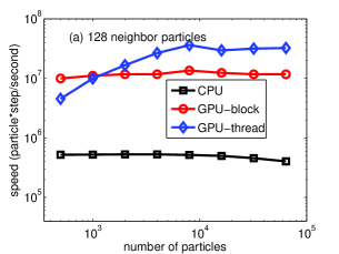
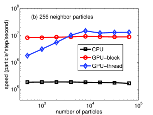
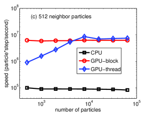
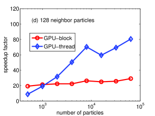
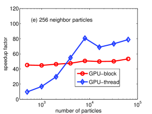
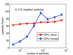
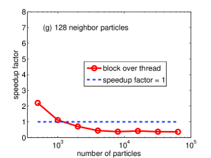
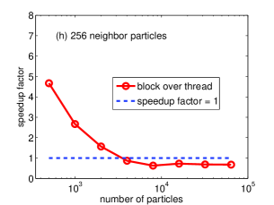
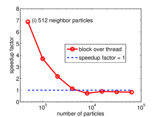
Figure 1: (Color online) Performance evaluation for the evolution part in the production stage for the LJ potential: (a-c) computation speeds for both the CPU code and the GPU code with different force evaluation schemes; (d-f) speedup factors of the GPU code over the CPU code; (g-i) relative speedup factors of the block-scheme over the thread-scheme. The maximal number of neighbor particles in the simulations (128, 256 or 512) are indicated in each subplot.

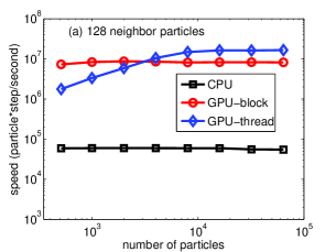
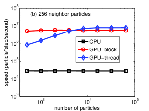
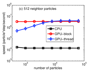
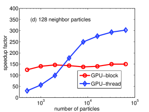
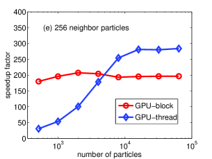
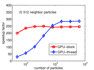
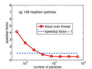
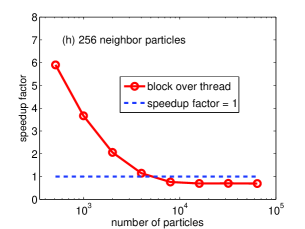
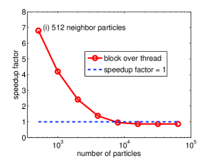
Figure 2: (Color online) Performance evaluation for the evolution part in the production stage for the RI potential: (a-c) computation speeds for both the CPU code and the GPU code with different force evaluation schemes; (d-f) speedup factors of the GPU code over the CPU code; (g-i) relative speedup factors of the block-scheme over the thread-scheme. The maximal number of neighbor particles in the simulations (128, 256 or 512) are indicated in each subplot.

In this subsection, we evaluate the performance of the evolution part, with an emphasis on the comparison of the two force evaluation schemes. To be specific, we only present the results for the production stage, where the heat current data need to be calculated and recorded. The results for the equilibration stage are similar. We test the performance for the evolution part by measuring the computation time for 1000 time steps. The computational speed is defined as the product of the number of particles and the number of steps divided by the computation time. In the literature [5, 8], the inverse of this quantity is also used to evaluate the computational speed. The speedup factor is defined to be the computation time for the CPU over that for the GPU. The system size used for our evaluation spans from a few hundred to 64 thousand particles. We also considered different cutoff radii, which determine the maximal number of neighbor particles $N_{m}$.

4.1.1 The LJ potential

The performances for the LJ potential are presented in Fig. 1, where the computational speeds and the speedup factors are plotted against the simulation size.

For our CPU code, the LJ potential with $N_{m}=128$ executes at a speed of about $5.0\times 10^{5}$ particle $\cdot$ step / second, or equivalently, 2.0 $\mu$s / (particle $\cdot$ step). The computational speed decreases with the increasing of the maximal number of neighbor particles $N_{m}$. For $N_{m}=512$, the computational speed slows down to about $9.0\times 10^{4}$ particle $\cdot$ step / second. For relatively small systems ($N<10^{4}$), the computation speed is nearly independent of the simulation size, indicating a good linear-scaling dependence of the computation time on the simulation size. However, the linear-scaling behavior is not well preserved for relatively large systems ($N>10^{4}$). This is probably due to the more expensive memory operations for larger data arrays associated with larger simulation size. We will come to this problem when we discuss the RI potential later.

Our GPU implementation achieves high performance and large speedup factors. By using the thread-scheme, the computational speed can be as high as $3.5\times 10^{7}$ particle $\cdot$ step / second, or equivalently, 0.029 $\mu$s / (particle $\cdot$ step) for $N_{m}=128$ and $N=8000$, which gives a speedup factor of about 70. For $N_{m}=512$ and $N=8000$, the speedup factor can reach 95 by using the thread-scheme.

From Fig. 1 (a-c) we can see that the computational speeds for the thread-scheme and the block-scheme saturate at different simulation sizes. As discussed before, the number of invoked blocks for the force evaluation kernel in the thread-scheme is $\lceil N/S_{b}\rceil$. With a block size of $S_{b}=128$, the number of blocks only reaches the upper bound of the number of resident blocks in the GPU when $N=16384$. This explains why the performance for the thread-scheme saturates at about $N=10^{4}$. In contrast, the number of invoked blocks for the force evaluation kernel in the block-scheme is the number of particles, and the block-scheme can attain its peak performance with only a few hundred particles.

There is always a crossover of the performances for the two force evaluation schemes. For the cases of $N_{m}$ = 128, 256 and 512, the simulation sizes at which the crossovers take place are around 1000, 3000 and 5000, respectively. From Fig. 1 (g-i) we can see that while the thread-scheme is a little faster when $N>10^{4}$, the block-scheme is several times faster when $N<10^{4}$. The smaller the system, the higher the relative speedup factor of the block-scheme over the thread-scheme. This makes the block-scheme more preferable for thermal conductivity calculation using the Green-Kubo method, where we rarely need to consider system with more than a few thousand particles. There are two main reasons for the superior performance of the thread-scheme over the block-scheme for large systems when saturation is obtained for both schemes. The first is that in the block-scheme, the total force and heat current for each particle has to be accumulated by binary reduction, during which only a portion of threads are used to do the calculation. The second is that there is more global memory access for the block-scheme. In the block-scheme, the positions $\mathbf{r}_{i}$ and velocities $\mathbf{v}_{i}$ as used in lines 5 and 6 of Algorithm 3 need to be transfered from global memory to all the threads in the block corresponding to the heading particle $i$. In contrast, in the thread-scheme, the positions and velocities for a heading particle need only to be transfered from global memory to a single thread.

From Fig. 1 (d-f) we can see that while the speedup factors for the thread-scheme nearly do not vary with the increasing of $N_{m}$, the speedup factors for the block-scheme increase significantly with the increasing of $N_{m}$. The computation time for the thread-scheme is dominated by the for loop in lines 4-12 of Algorithm 2 and scales nearly linearly with respect to $N_{m}$, as in the case of the CPU code. In contrast, in the block-scheme, a significant portion of computation time is spent on the extra global memory access of positions and velocities and the binary reduction operations for force and heat current. The amount of the extra global memory access scales with $N$ and the number of binary reduction operations is determined by $S_{b}$, both of which do not scale with $N_{m}$. Thus, the block-scheme performs better and better with the increasing of $N_{m}$.

Lastly, we note that there is an abrupt ‘drop’ of the computational speed for the thread-scheme around $N=10^{4}$. This is likely caused by increasingly inefficient use of the cache memories and the saturation of the GPU’s cores.

4.1.2 The RI potential

The RI potential is much more computationally intensive than the LJ potential. One can see from Fig. 2 (a) that for $N_{m}$ = 128, the CPU computational speed for the RI potential is about $6\times 10^{4}$ particle $\cdot$ step / second, or equivalently, 17 $\mu$s / (particle $\cdot$ step), which is about 12 times slower than that for the LJ potential with the same $N_{m}$. Thus, compared to the LJ potential, the computation time for the RI potential would be dominated by the actual floating point operations, and this can help to understand why the linear-scaling behavior with respect to the simulation size is preserved much better for the RI potential (Fig. 2 (a-c)) than for the LJ potential (Fig. 1 (a-c)).

As for the performances for the GPU code, the results for the RI potential are even more impressive compared with the LJ potential. The speedup factors can be as large as 300 for the thread-scheme. The higher acceleration rate for the RI potential compared to that for the LJ potential results from the higher arithmetic intensity of RI potential.

The testing results for the RI potential exhibit similar features as in the case of the LJ potential, which can be listed as follows:

1. The performance for the thread-scheme saturates only when $N>10^{4}$, while that for the block-scheme saturates for a few hundred particles.

2. For each $N_{m}$, there is a crossover point for the performance curves, before which the block-scheme performs better, and after which the opposite is true. The simulation sizes associated with the crossover points are around 2000, 5000 and 7000 for $N_{m}$ = 128, 256 and 512, respectively.

3. The performance for the thread-scheme is weakly dependent on the value of $N_{m}$. In contrast, the average speedup factor for the block-scheme varies from 150 to 200 to 250 when $N_{m}$ increases from 128 to 256 to 512.

All these points can be explained similarly as in the case of the LJ potential.

4.2 Neighbor list construction

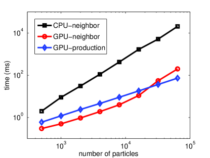
Figure 3: Computation times for the neighbor list construction in the CPU and the GPU as a function of the simulation size. The computation time of 10 production steps without neighbor list update in the block-scheme for LJ potential with $N_{m}$ = 128 is also presented for comparison.

The computation times for constructing the neighbor list in the CPU and the GPU are compared in Fig. 3. The computation time for the CPU implementation scales quadratically with the simulation size, as expected. Although our GPU implementation is nearly a direct translation of the CPU implementation, its computation time scales linearly for $N<10^{4}$ and only begin to scale quadratically for $N>10^{4}$. Furthermore, for $N<10^{4}$, the computation time for the neighbor list construction is less than that of 10 production steps without neighbor list update in the block-scheme for LJ potential with $N_{m}$ = 128. As a comparison, the computation time for the neighbor list construction reported by Anderson et al [5], who use a cell decomposition approach, is about 10 times larger than their reported computation time for the force evaluation with one step. Thus, for $N<10^{4}$, the simple neighbor list construction method as given in Algorithm 1 can lead to rather good performance. However, for larger systems, the cell decomposition approach will definitely perform better.

4.3 HCACF calculation

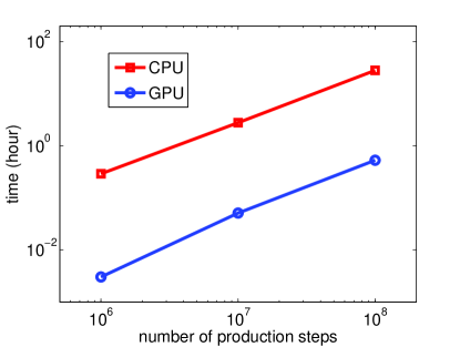
Figure 4: (Color online) Computation times for the HCACF calculations in CPU and GPU as functions of the production time steps $N_{p}$. The number of data points for HCACF is chosen to be $N_{c}=5\times 10^{4}$.

Figure 4 presents the computation times for the HCACF calculation in the CPU and the GPU. The calculation of HCACF for the case of $N_{c}=5\times 10^{4}$ and $N_{p}=10^{8}$ takes up more than one day using a CPU but only half an hour using a GPU. From the previous discussion, we can see that the evolution part of the MD simulation achieves more than two orders of magnitude speedup. If we do not implement this post-processing part in the GPU as well, the speedup factor for the whole program will be much lower than that for the evolution part alone. For example, in the next section, we will apply the GPU code in the block-scheme to calculate the thermal conductivity of PbTe at a given temperature using the following values of the relevant parameters: $N=512$, $N_{m}=512$ and $N_{p}=10^{8}$. The computational speed is $3.4\times 10^{6}$ particle $\cdot$ step / second by using the block-scheme (Fig. 2 (c)), and the computation time for the evolution part would be less than 5 hours, which is even much less than that for the HCACF calculation in CPU.

5 Validation

In this section, we validate our GPU implementation by studying the lattice thermal conductivity of solid argon and bulk PbTe, using the LJ potential and the RI potential, respectively.

5.1 Determining the lattice constant at zero pressure

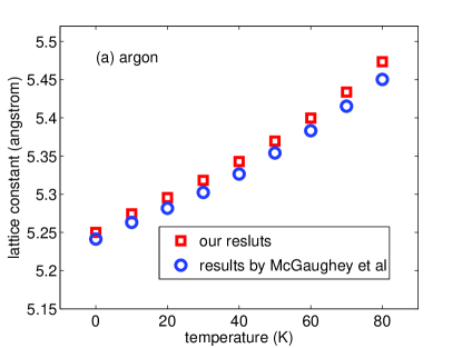
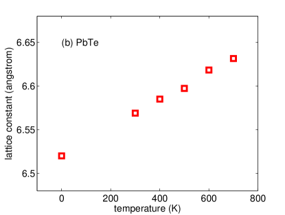
Figure 5: (Color online) Zero-pressure lattice constants for solid argon (a) and PbTe (b) at different temperatures. For solid argon, the results by McGaughey et al [20] are also presented for comparison.

We only consider systems without external pressure (0 Pa). The correct determination of the lattice constant is crucial for the correct prediction of the lattice thermal conductivity. In fact, the under-prediction of the lattice thermal conductivities of solid argon [19] compared to experimental data results from an over-prediction of the lattice constants, which is corrected by later studies [20, 21, 22, 23]. The zero-pressure lattice constant for non-bonded potential can be obtained by using an NPT ensemble to control the pressure as well as the temperature of a sufficiently large system with a large cutoff radius for force evaluation. The calculated lattice constants at different temperatures for solid argon and PbTe are shown in Fig. 5. For solid argon, the results by McGaughey et al [20] are also presented for comparison. The lattice constants at zero temperature are obtained from the cohesive energy curves. For solid argon, the zero-temperature lattice constant is calculated to be 5.25 Å. As a comparison, the one obtained by McGaughey et al [20] is 5.24 Å, and the experimental value [36] is 5.30 Å. For PbTe, the zero-temperature lattice constant is calculated to be 6.52 Å, which is the same as that obtained by Qiu et al [31]. The lattice constants for PbTe at elevated temperatures also exhibit a linear-dependence behavior on temperature in the range of 300-700 K, from which we can deduce a well defined value of the thermal expansion coefficient, $2.30\times 10^{-5}$ K^-1, which is comparable to the experimental value [37], $2.04\times 10^{-5}$ K^-1.

5.2 Results for lattice thermal conductivities

After determining the lattice constants, we can calculate the zero-pressure lattice thermal conductivities at different temperatures. For argon, the cutoff radius for force evaluation is chosen to be $R_{c}=3\sigma$ and the time step is chosen to be $\delta t=2$ fs. We firstly equilibrate the simulated system in the NVT ensemble for $N_{e}=10^{6}$ steps and then evolve the system in the NVE ensemble for $N_{p}=10^{7}$ steps. The NVT ensemble in the equilibration stage serves to control the temperature of the simulated system. After the system attains an equilibrated temperature, the heat current data are calculated and recorded at each time step in the NVE ensemble, which is the most natural ensemble to simulate an equilibrated system (with fluctuations, of course). For PbTe, the corresponding parameters are chosen to be $R_{c}=16$ Å, $\delta t=0.2$ fs, $N_{e}=10^{7}$ and $N_{p}=10^{8}$. Another parameter which is only relevant for PbTe, namely, the electrostatic damping factor, is chosen to be $\alpha=0.2$ Å^-1, which is a reasonable choice as suggested by Fennell et al [27].

5.2.1 Solid argon

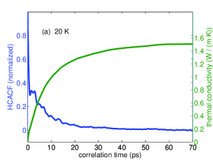
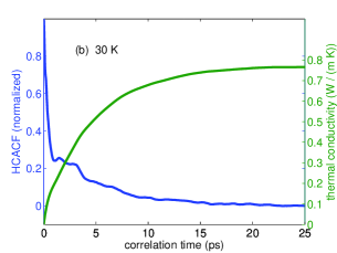
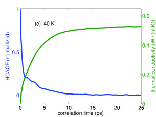
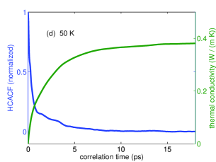
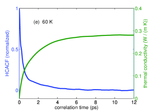
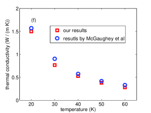
Figure 6: (Color online) HCACFs and RTCs (a-e) of solid argon as a function of the correlation time and the converged lattice thermal conductivity as a function of temperature (f). In (f), the MD results obtained by McGaughey et al [20] are also presented for comparison.

Figure 6 (a-e) gives the calculated results for HCACFs and RTCs at different temperatures for solid argon using the GPU code in the block-scheme. For all the temperatures, well converged HCACF and RTC can always be obtained, as long as we collect sufficiently many heat current data. The curves presented in Fig 6 (a-e) are obtained by setting the number of production steps to be $N_{p}=10^{7}$. Since the curves are so smooth, we need not do any fitting to obtain a well defined value of thermal conductivity.

Figure 6 (f) compares our simulation results with those reported by McGaughey et al [20]. We have tested the finite size effects and found that a simulation size of $N=5\times 5\times 5\times 4=500$ is sufficient. It can be seen that our results agree well with theirs. Since their results are well established, this agreement provides a strong evidence of the correctness of our program.

5.2.2 PbTe

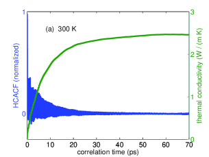
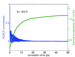
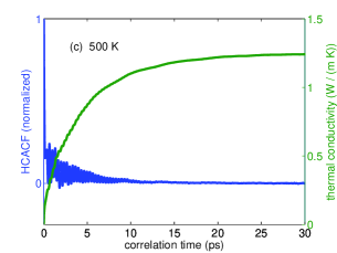
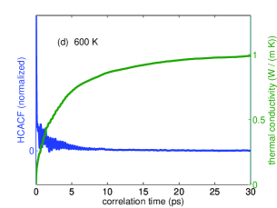
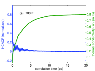
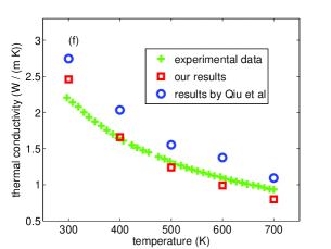
Figure 7: (Color online) HCACFs and RTCs (a-e) of PbTe as a function of the correlation time and the converged lattice thermal conductivity as a function of temperature (f). In (f), experimental data [38] and the MD results obtained by Qiu et al [30] are also presented for comparison.

The calculated HCACFs and RTCs at different temperatures for PbTe using the GPU code in the block-scheme are presented in Fig 7 (a-e). For PbTe, a number of $10^{7}$ production steps is not sufficient to obtain smooth curves for HCACF and RTC. The curves presented in Fig 7 (a-e) are obtained by setting the number of production steps to be $N_{p}=10^{8}$. It can be seen that even if there exists high frequency oscillations (caused by optical phonons [28]) in the HCACF, the RTC still exhibits a very smooth behavior as long as we collect sufficiently many heat current data.

Figure 7 (f) presents our calculated lattice thermal conductivities of PbTe at different temperatures. We have tested the size effects and found that a simulation size of $N=4\times 4\times 4\times 8=512$ is sufficient. Our results agree well with the original results obtained by Qiu et al [30]. Both results agree fairly with the experimental data [38].

5.3 A demonstration of the finite-size effect

We stressed several times that the Green-Kubo method requires only small system sizes for well-converged results. Now, we give a demonstration of this important fact. Figure 8 presents the calculated thermal conductivities of solid argon at zero pressure and 10 K with different simulation sizes: $N=$ 32, 108, 256, 500, 864, and 1372. We choose to demonstrate the finite-size effect for the lowest temperature case, since this case gives the largest value of thermal conductivity (and phonon mean free path), and a system with larger thermal conductivity usually presents more prominent finite-size effect. From Fig. 8 we see that, the finite-size effect can be eliminated even by using a system of 256 argon atoms. The small finite-size effect is one of the most advantages of the Green-Kubo method over the direct method, and makes our new force evaluation scheme (the block-scheme) very useful.

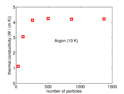
Figure 8: (Color online) Lattice thermal conductivity of solid argon at 0 Pa and 10 K as a function of the simulation size.

6 Conclusions

In conclusion, we presented in detail the development and optimization of a molecular dynamics simulation program fully implemented in the GPU, which can calculate the lattice thermal conductivity using the Green-Kubo formula. For the most time-consuming part, the force evaluation part, we compared two alternative approaches, a thread-scheme where the total force for a particle is accumulated in a single thread and a block scheme where the pair forces for a particle are distributively calculated in different threads within a block and summed up using shared memory to obtain the total force of the given particle. For both LJ and RI potentials, the block-scheme outperforms the thread-scheme for smaller systems. This makes the block-scheme particularly preferable for thermal conductivity calculations using the Green-Kubo approach, which is more demanding on the simulation time rather than the simulation size. For large systems, the speedup factors obtained reach about one hundred and three hundred for LJ and RI potentials, respectively. The higher acceleration rate for the RI potential compared with that for the LJ potential results from its higher arithmetic intensity, defined as the number of arithmetic operations divided by the number of memory operations. The correctness of our implementation is validated by calculating the lattice thermal conductivities of solid argon and PbTe.

Both the LJ and the RI potentials considered in this work are very simple; they are pair-wise in nature. Generalization of our work to more general and complicated potentials deserves further consideration. It is interesting to consider the acceleration of the bond-order potential, which would find interesting applications in carbon nanostructures. Since the bond-order potential also has high arithmetic intensity, we expect that a well-designed GPU implementation of the bond-order potential can also lead to high acceleration rates.

In this work, we only applied our MD program to thermal conductivity calculations. However, our program contains most of the essential parts of a general MD program. Thus, one can modify it to study other problems. Our code is available upon request.

References

- Belleman et al. [2008] R. G. Belleman, J. Bedorf, S. F. P. Zwart, High performance direct gravitational -body simulations on graphics processing units - II: an implementation in CUDA, New Astronomy 13 (2008) 103–112.
- Yang et al. [2007] J. Yang, Y. Wang, Y. Chen, GPU accelerated molecular dynamics simulation of thermal conductivities, J. Comp. Phys. 221 (2007) 799–804.
- Stone et al. [2007] J. E. Stone, J. C. Phillips, P. L. Freddolino, D. J. Hardy, L. G. Trabuco, K. Schulten, Accelerating molecular modeling applications with graphics processors, J. Comp. Chem. 28 (2007) 72618–2640.
- van Meel et al. [2008] J. A. van Meel, A. Arnold, D. Frenkel, S. F. Portegies Zwart, R. G. Belleman, Harvesting graphics power for MD simulations, Molecular Simulation 34 (2008) 259–266.
- Anderson et al. [2008] J. A. Anderson, C. D. Lorenz, A. Travesset, General purpose molecular dynamics simulations fully implemented on graphics processing units, J. Comp. Phys. 227 (2008) 5342–5359.
- Liu et al. [2008] W. Liu, B. Schmidt, G. Voss, W. Müller-Wittig, Accelerating molecular dynamics simulations using graphics processing units with CUDA, Comp. Phys. Commun. 179 (2008) 634–641.
- Friedrichs et al. [2009] M. S. Friedrichs, P. Eastman, V. Vaidyanathan, M. Houston, S. Legrand, A. L. Beberg, D. L. Ensign, C. M. Bruns, V. S. Pande, Accelerating molecular dynamic simulation on graphics processing units, J Comput Chem. 30 (2009) 864–872.
- Rapaport [2011] D. C. Rapaport, Enhanced molecular dynamics performance with a programmable graphics processor, Comp. Phys. Commun. 182 (2011) 926–934.
- Preis et al. [2009] T. Preis, P. Virnau, W. Paul, J. J. Schneider, GPU accelerated Monte Carlo simulation of the 2D and 3D Ising model, J. Comp. Phys. 228 (2009) 4468–4477.
- Anderson et al. [2007] A. G. Anderson, W. A. Goddard, P. Schröder, Quantum Monte Carlo on graphical processing units, Comp. Phys. Commun. 177 (2007) 298–306.
- Ihnatsenka [2012] S. Ihnatsenka, Computation of electron quantum transport in graphene nanoribbons using GPU, Comp. Phys. Commun. 183 (2012) 543–546.
- Siro and Harju [2012] T. Siro, A. Harju, Exact diagonalization of the Hubbard model on graphics processing units, Comp. Phys. Commun. 183 (2012) 1884–1889.
- Yao et al. [2005] Z. Yao, J. S. Wang, B. Li, G. R. Liu, Thermal conduction of carbon nanotubes using molecular dynamics, Phys. Rev. B 71 (2005) 085417.
- Schelling et al. [2002] P. K. Schelling, S. R. Phillpot, P. Keblinski, Comparison of atomic-level simulation methods for computing thermal conductivity, Phys. Rev. B 65 (2002) 144306.
- Sellan et al. [2010] D. P. Sellan, E. S. Landry, J. E. Turney, A. J. H. McGaughey, C. H. Amon, Size effects in molecular dynamics thermal conductivity predictions, Phys. Rev. B 81 (2010) 214305.
- Green [1954] M. S. Green, Markoff random processes and the statistical mechanics of time-dependent phenomena. II. irreversible processes in fluids, J. Chem. Phys. 22 (1954) 398.
- Kubo [1957] R. Kubo, Statistical-mechanical theory of irreversible processes. I. general theory and simple applications to magnetic and conduction problems, J. Phys. Soc. Jpn. 12 (1957) 570.
- McQuarrie [2000] D. A. McQuarrie, Statistical Mechanics, University Science Books, Sausalito, 2000.
- Kaburaki et al. [1999] H. Kaburaki, J. Li, S. Yip, Thermal conductivity of solid argon by molecular dynamics, Mater. Res. Soc. Symp. Proc. 538 (1999) 503.
- McGaughey and Kaviany [2004] A. J. H. McGaughey, M. Kaviany, Thermal conductivity decomposition and analysis using molecular dynamics simulations, Int. J. Heat Mass Transfer 47 (2004) 1783.
- Tretiakova and Scandolo [2004] K. V. Tretiakova, S. Scandolo, Thermal conductivity of solid argon from molecular dynamics simulations, J. Chem. Phys. 120 (2004) 3765.
- Chen et al. [2004] Y. Chen, J. R. Lukes, D. Li, J. Yang, Y. Wu, Thermal expansion and impurity effects on lattice thermal conductivity of solid argon, J. Chem. Phys. 120 (2004) 3841.
- Kaburaki et al. [2007] H. Kaburaki, J. Li, S. Yip, H. Kimizuka, Dynamical thermal conductivity of argon crystal, J. Appl. Phys. 102 (2007) 043514.
- Chen et al. [2005] Y. Chen, D. Li, J. R. Lukes, Z. Ni, M. Chen, Minimum superlattice thermal conductivity from molecular dynamics, Phys. Rev. B 72 (2005) 174302.
- Landry et al. [2008] E. S. Landry, M. I. Hussein, A. J. H. McGaughey, Complex superlattice unit cell designs for reduced thermal conductivity, Phys. Rev. B 77 (2008) 0184302.
- Wolf et al. [1999] D. Wolf, P. Keblinski, S. R. Phillpot, J. Eggebrecht, Exact method for the simulation of coulombic systems by spherically truncated, pairwise summation, J. Chem. Phys. 110 (1999) 8255.
- Fennell and Gezelter [2006] C. J. Fennell, J. D. Gezelter, Is the Ewald summation still necessary? pairwise alternatives to the accepted standard for long-range electrostatics, J. Chem. Phys. 124 (2006) 234104.
- McGaughey and Kaviany [2004] A. J. H. McGaughey, M. Kaviany, Thermal conductivity decomposition and analysis using molecular dynamics simulations, Int. J. Heat Mass Transfer 47 (2004) 1799–1816.
- Kulkarni and Zhou [2006] A. J. Kulkarni, M. Zhou, Size-dependent thermal conductivity of zinc oxide nanobelts, Appl. Phys. Lett. 88 (2006) 141921.
- Qiu et al. [2012] B. Qiu, H. Bao, G. Zhang, Y. Wu, X. Ruan, Molecular dynamics simulations of lattice thermal conductivity and spectral phonon mean free path of PbTe: Bulk and nanostructures, Comp. Mater. Sci. 53 (2012) 278–285.
- Qiu et al. [2008] B. Qiu, H. Bao, X. Ruan, Multiscale simulations of thermoelectric properties of PbTe, ASME 2008 3rd Energy Nanotechnology International COnference (2008) 45.
- Che et al. [2000] J. Che, T. Cagin, W. Deng, W. A. Goddard, Thermal conductivity of diamond and related materials from molecular dynamics simulations, J. Chem. Phys. 113 (2000) 6888.
- Henry and Chen [2008] A. Henry, G. Chen, High thermal conductivity of single polyethylene chains using molecular dynamics simulations, Phys. Rev. Lett. 101 (2008) 235502.
- NVIDIA [2011] NVIDIA, CUDA C programming guide, version 4.0 (2011).
- Verlet [1967] L. Verlet, Computer ‘experiments’ on classical fluids. I. thermodynamical properties of Lennard-Jones molecules, Phys. Rev. 159 (1967) 98–103.
- Ashcroft and Mermin [1976] N. W. Ashcroft, N. D. Mermin, Solid State Physics, Saunders College, Orlando, FL, 1976.
- Houston et al. [1968] B. Houston, R. Strakna, H. Belson, Elastic constants, thermal expansion, and Debye temperature of lead telluride, J. Appl. Phys. 39 (1968) 3913–3916.
- Fedorov and Machuev [1969] V. I. Fedorov, V. I. Machuev, The thermal conductivity of PbTe, SnTe, and GeTe in the solid and liquid phases, Sov. Phys. Solid State, USSR 11 (1969) 1116.