On the resonant optical bistability condition.

Abstract

We address a two level system in an environment interacting with the electromagnetic field in the dipole approximation. The resonant optical bistability induced by local-field effects is studied by considering the relationship between the population difference and the excitation field. The diversity of various systems is included by accounting for the system self-action via the surface part of the Green’s dyadic in the general form. The bistability condition and the exact solution of the steady state optical Bloch equations at the absolute bistability threshold are derived analytically.

Because of its underlying nature and possible applications in the field of all-optical processing, the optical bistability (OB) was a subject of an intense experimental and theoretical research.Abraham82 ; Gibbs85 In the early studies the use of a saturable absorber to induce OB was suggested.Szoke69 ; Austin71 ; Spiller71 ; McCall74 ; Bonifacio76 The phenomenon was demonstrated experimentally for a cell of sodium vapor enclosed in a Fabry Perot interferometer and excited by a cw dyelaser.Gibbs76 Later it was conjectured that the local-field corrections alone could give rise to the mirrorless OB. Bowden79 This type of bistability was extensively studiedAbram82 ; Hopf84 ; BenAryeh86 ; Friedberg89 ; Crenshaw92 and observed experimentally.Hehlen94

The practical interest in all-optical devices faded to some extent as their solid state counterparts proved to perform better in terms of the switching speed and device density. However, the OB and optical hysteresis remain of considerable interest from the fundamental standpoint as a clear manifestation of a nonlinear light-matter interaction. Some new types of bistability mechanisms were discussed recently.Afanasev99 ; Kaplan08 ; Kaplan09 ; Volkov10 Besides, the question of the OB and hysteresis has received a renewed attention in connection with novel hybrid 0D nanoscopic systems, e. g., an artificial molecules comprising a semiconductor quantum dot (SQD) and metal nanoparticles (see Refs. Zhang06, ; Artuso08, ; Sadeghi10b, ; Malyshev11, and references therein).

In this paper we address only the mirrorless OB induced by the local-field effects on a two-level system (TLS) interacting with the electromagnetic field in the dipole approximation. The local-filed correction leads to a self-action of the system, which results in a nonlinear relation between the applied field and the one acting upon the system. This type of the OB mechanism can be relevant for a large variety of systems: dense 3D assemblies of two-level atoms Bowden79 ; Friedberg89 , optically dense thin films of TLS Zakharov88 ; Benedict90 or films of linear molecular aggregates, Malyshev96 ; Klugkist07 ; Klugkist08 hybrid metal-semiconductor systems, Zhang06 ; Artuso08 ; Sadeghi10b ; Malyshev11 or a more general case of a TLS in an environment involving dielectric and conducting surfaces, such as, a stratified media, a microcavity or a nanostructure.

OB can occur within a range of internal system parameters and external field intensities; identifying these ranges is therefore an important problems and its analytical solution is desirable. To the best of the author’s knowledge, so far, it has been solved exactly only for two particular cases. Thus, Friedberg et al obtained analytically the bistability condition for the limiting case in which the active mechanism of the feedback is the nonlinear Lorentz shift of the resonance in a 3D gas of two-level atoms, which resulted from the near-field corrections. Friedberg89 Ignoring these corrections, Zakharov and Manykin derived the exact bistability criterion in the other limit in which the self-action is due to the radiated secondary field in a thin 2D film of TLS. Zakharov88 The case when both these fields contribute into the self-action has been studied only numerically so far. Orayevsky94

We consider the simplest optical TLS coupled to an environment. The self-action of the TLS due to the environment can be described by the surface part of the Green’s dyadic evaluated at the position of the TLS. Therefore, in this case the nonlinearity is characterized by a complex number which should satisfy some condition for the OB to occur. Below, we derive such condition analytically.

Following Refs. Friedberg89, ; Zakharov88, ; Orayevsky94, we address the OB condition by considering the relationship between the population difference and the excitation field within the framework of the Bloch equations for the $2\times 2$ density matrix $\rho_{mn}\>(m,n=0,1)$ of a TLS. In the rotating wave approximation these equations read:

$$\dot{Z} =-\gamma\,(Z+1)-\frac{1}{2}\left[\,\Omega\,P^{*}+\Omega^{*}P\,\right]\ ,$$ (1a)

$$\dot{P} =-(\Gamma+i\,\Delta)\,P+\Omega\,Z\ ,$$ (1b)

where $Z=\rho_{11}-\rho_{00}$ is the population difference between the excited and the ground state of the TLS, $P$ is the amplitude of the off-diagonal density matrix element defined through $\rho_{10}=-(i/2)P\exp(-i\omega t)$, $\gamma$ and $\Gamma$ are the relaxation constants of the population and the dipole moment, respectively, $\Delta=\omega_{0}-\omega$ is the detuning of the driving field frequency $\omega$ from the TLS resonance $\omega_{0}$, and $\Omega={\bm{\mu}\bf E}/\hbar$ is the total electric field $\bf E$ (in frequency units) acting upon the system, while $\bm{\mu}$ being the TLS optical transition dipole. The dipole moment of the system is ${\bf p}=-i\,P{\bm{\mu}}$, where $P$ is its complex amplitude.

To calculate the total field $\Omega$ the Maxwell’s equations are to be solved for a particular geometry. However, for a single dipole in an environment the total field $\Omega$ can be represented in the following general form:

$$\Omega=\widetilde{\Omega}_{0}+\Omega_{2},\quad\Omega_{2}=-i\,G\,P$$ (2)

where $\widetilde{\Omega}_{0}$ is the renormalized incident field and $\Omega_{2}$ is the secondary dipole field. The latter field is due to the feedback of the environment and is related to the corresponding response functionAgarwal75a ; Agarwal75b ; Agarwal98 . It is determined by the surface part of the Green’s dyadic evaluated at the position of the dipole. The near-zone component of the secondary dipole field, governed by $\mathrm{Re}(G)$, can originate from the near-field corrections, Friedberg89 while the far-zone contribution, governed by $\mathrm{Im}(G)$, can be due to the radiation. Zakharov88 In hybrid nano-systems comprising a SQD, the feedback is provided by the secondary reflected field of the optical transition dipole moment. Thus, independently of its physical mechanism, the self-action is determined by the single complex valued parameter $G$. The total field $\Omega$ acting upon the TLS depends therefore on its state. Together with the nonlinearity of the TLS that can give rise to a variety of effects, such as the OB.

Figure 1: The RHS of Eq. (3a) for $G=6$, $\Delta=1$ (solid line), $G=4$, $\Delta=1$ (dashed line) and $G=8\,i$, $\Delta=0$ (dotted line)

Under the steady-state conditions Eqs. (1) read:

$$\frac{|\widetilde{\Omega}_{0}|^{2}}{\gamma\,\Gamma} =-\frac{Z+1}{Z}\>\frac{(\Gamma-G_{\mathrm{I}}Z)^{2}+(\Delta+G_{\mathrm{R}}Z)^{2}}{\Gamma^{2}}\ ,$$ (3a)

$$P =\frac{Z\;\widetilde{\Omega}_{0}}{(\Gamma-G_{\mathrm{I}}\,Z)+i\,(\Delta+G_{\mathrm{R}}\,Z)}\ ,$$ (3b)

where $G_{\mathrm{R}}=\mathrm{Re}(G)$ and $G_{\mathrm{I}}=\mathrm{Im}(G)$. The above equation highlights a known result of cavity quantum electrodynamics: the real part of the Green’s dyadic shift the frequency while the imaginary part renormalizes the decay rate.Agarwal75a ; Agarwal75b ; Agarwal98 Both effects can be active mechanisms of the OB.

Eq. (3a) is of the third order in $Z$ and can therefore have three real roots for some values of $\Delta$, $\Gamma$, $G_{\mathrm{R}}$, and $G_{\mathrm{I}}$ ($\Gamma$ is used as a unit rate from now on). These three solutions are different when the right hand side (RHS) of Eq. (3a) has a minimum and a maximum (see the solid line in Fig. 1), corresponding to two real roots of the RHS derivative, which satisfy the following equation

$$2\,|G|^{2}\,Z^{3}+(|G|^{2}+2\,G_{\mathrm{R}}\,\Delta-2\,G_{\mathrm{I}})\,Z^{2}-(1+\Delta^{2})=0\ .$$ (4)

A threshold for bistability occurs when Eq. (4) has a double root (merged extrema – see the dashed or dotted lines in Fig. 1). In this case the solutions of Eq. (3a) are:

$$Z_{1}=Z_{2}=-\frac{|G|^{2}+2\,(G_{\mathrm{R}}\Delta-G_{\mathrm{I}})}{3\;|G|^{2}}\ ,\quad Z_{3}=-\frac{Z_{1}}{2}$$ (5)

Using the above root $Z_{1,2}$ and the condition $-1\leq Z\leq 0$ one obtains an important constraint for the detuning $\Delta$:

$$G_{\mathrm{R}}\,\Delta-G_{\mathrm{I}}\leq|G|^{2}$$ (6)

The formal condition of the existence of the double root (5) is determined by the following equation on $\Delta$:

$$\left(|G|^{2}+2\,G_{\mathrm{R}}\,\Delta-2\,G_{\mathrm{I}}\right)^{3}-27\,|G|^{4}\,(1+\Delta^{2})=0\ ,$$ (7)

which is cubic in $\Delta$ and can also have three real solutions. It can be shown that only two of them, say $\Delta_{1}<\Delta_{2}$, satisfy the constraint (6) and yield the upper and lower threshold values of the population difference $Z$ and the external field $\widetilde{\Omega}_{0}$. Therefore, Eq. (4) has three different real roots within a window of detunings $\Delta_{1}\leq\Delta\leq\Delta_{2}$. The absolute bistability threshold occurs when the window shrinks into a point, i. e., when a degenerate root $\Delta_{1}=\Delta_{2}$ of Eq. (7) appears. After some algebra, one can obtain the following alternative for the existence of such double root:

$$G_{\mathrm{R}}^{4}+2\,(G_{\mathrm{I}}^{2}-4\,G_{\mathrm{I}}-8)\,G_{\mathrm{R}}^{2}+G_{\mathrm{I}}^{3}\,(G_{\mathrm{I}}-8) =0\ ,$$ (8a)

$$G_{\mathrm{I}}+1 =0\ .$$ (8b)

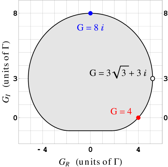
Figure 2: The stability phase map: outside the gray area the system can be bistable. Solid line represents the phase boundary given by Eq. (9). See text for more details.

Only two of the solutions of the biquadratic equation (8a) satisfy the constraint (6). Analyzing the roots of Eq. (4) in the vicinity of the solution to Eqs. (8b) and (7), one finds that the system can be bistable below the line given by $G_{\mathrm{I}}=-1$, while being critical (i. e., $Z_{1,2}=-1$) on the line for $|G_{\mathrm{R}}|\leq\sqrt{3}$. Finally, the absolute bistability threshold is:

$$G_{\mathrm{R}}^{2}=8+4\,G_{\mathrm{I}}-G_{\mathrm{I}}^{2}+8\sqrt{1+G_{\mathrm{I}}}, \;-1<G_{\mathrm{I}}\leq 8$$ (9a)

$$-\sqrt{3}\leq G_{\mathrm{R}}\leq\sqrt{3}, \qquad\;\;G_{\mathrm{I}}=-1$$ (9b)

For completeness, we provide also the expression for the corresponding detuning:

$$\Delta=\frac{|G|^{4}-4\,G_{\mathrm{R}}^{2}\,(G_{\mathrm{I}}+3)-4\,G_{\mathrm{I}}^{2}\,(G_{\mathrm{I}}-1)}{|G|^{4}+8\,G_{\mathrm{I}}\,\left[\,G_{\mathrm{I}}^{3}+G_{\mathrm{R}}^{2}\,(G_{\mathrm{I}}+2)\,\right]}\;G_{\mathrm{R}}\ .$$ (10)

Equation (9) provides the condition of existence of three real roots of Eq. (3a). We studied the stability of these by analyzing Lyapunov exponents of Eqs. (1) in the vicinity of a stationary solution and calculated the stability phase map numerically. Figure 2 shows such phase diagram in the space of the feedback parameter $G$. Three different real solutions of Eq. (3a) exist within the white area, two of them being stable. The line dividing the two phases represents the analytical condition Eq. (9) which gives also the bistability threshold. The general criterion Eq. (9) recovers both reported exact results: $G_{\mathrm{I}}>8$ for $G_{\mathrm{R}}=0$ Zakharov88 and $G_{\mathrm{R}}>4$ for $G_{\mathrm{I}}=0$ Friedberg89 (the corresponding threshold values of $G$ are marked by full circles in Fig. 2). Note the mirror symmetry of the bistability map with respect to the line $G_{\mathrm{R}}=0$, which reflects the invariance of Eq. (3a) under the simultaneous change of signs of $G_{\mathrm{R}}$ and $\Delta$ Orayevsky94 .

Eqs. (5) and (10) give the full solution of the steady state problem at a bistability threshold, while Eq. (9) is the bistability condition, which constitute the main result of the paper.

Finally, we note that novel hybrid plasmonic nano systems, such as a SQD and a metal nanoparticle complex (see Ref. Malyshev11, and references therein) or a SQD embedded in a stratified medium are excellent model systems with adjustable nonlinearity. The self-action field in these complexes is the secondary reflected field of the SQD optical transition dipole moment acting back upon the SQD. In the most general case such environment feedback results in a complex self-action parameter $G$ which can be engineered by an appropriate choice of materials, geometry and/or external control parameters. Thus, if the SQD transition frequency is far from the plasmon resonance of the system then, typically, $|G_{\mathrm{R}}|\gg|G_{\mathrm{I}}|$ and the dominant mechanism of the bistability is the nonlinear Lorentz shift Friedberg89 . If the excitation frequency is near the surface plasmon resonance then the feedback can be almost purely imaginary: $|G_{\mathrm{I}}|\gg|G_{\mathrm{R}}|$ with $G_{\mathrm{I}}>0$. Algebraically, this case is equivalent to the one of the radiation induced self-action Zakharov88 . A very interesting case is $G_{\mathrm{I}}<0$ which can hardly be realized in the traditional extended 3D or 2D systems of two-level atoms. Nanoscopic hybrids are much more promising from this point of view due to their greater diversity. In the latter case various instabilities such as auto-oscillations can be expected under steady-state excitation. However, the detailed study of these instabilities goes beyond the scope of the present contribution and will be analyzed elsewhere.

Summarizing, we addressed the mirrorless resonant optical bistability of a two-level system in an environment by considering the relationship between the population difference and the intensity of the excitation field. The feedback of the environment was introduced in a general from via the surface part of the Green’s dyadic. We derived the analytical bistability condition and obtained the exact steady state solution of the Maxwell-Bloch equations at the absolute bistability threshold. Our findings open the possibility to easily analyze diverse physical systems, determine experimental conditions (such as, the appropriate detuning from the bare resonance and the intensity of the external field) necessary to observe the bistability and other nonlinear optical effects, as well as design and engineer new systems with desirable nonlinear optical properties.

I Acknowledgments

Support from the project MOSAICO (FIS2006-01485), fruitful discussions with V. A. Malyshev and the hospitality of the University of Groningen are gratefully acknowledged.

References

- (1) E. Abraham and S. D. Smith, Rep. Prog. Phys. 45, 815 (1982)
- (2) H. M. Gibbs, Optical bistability: controlling light with light (Academic Press, New York, 1985)
- (3) A. Szöke, V. Danen, J. Goldhar, and N. A. Kurnit, Appl. Phys. Lett. 15, 376 (1969).
- (4) J. W. Austin and L. G. DeShazer, J. Opt. Soc. Am. 61, 650 (1971).
- (5) E. Spiller, J. Opt. Soc. Am. 61, 699 (1971).
- (6) S. L. McCall, Phys. Rev. A 9, 1515 (1974).
- (7) R. Bonifacio and L. A. Lugiato, Opt. Commun. 19, 172 (1976).
- (8) H. M. Gibbs, S. L. McCall, and T. N. C. Venkatesan, Phys. Rev. Lett. 36, 1135 (1976).
- (9) C. M. Bowden and C. C. Sung, Phys. Rev. A 19, 2392 (1979).
- (10) I. Abram and A. Maruani, Phys. Rev. B 26, 4759 (1982).
- (11) F. A. Hopf, C. M. Bowden, and W. H. Louisell, Phys. Rev. A 29, 2591 (1984)
- (12) Y. Ben-Aryeh, C. M. Bowden, and J. C. Englund, Phys. Rev. A 34, 3917 (1986).
- (13) M. E. Crenshaw, M. Scalora, and C. M. Bowden, Phys. Rev. Lett. 68, 911 (1992).
- (14) R. Friedberg, S. R. Hartmann, and J. T. Manassah, Phys. Rev. A 39, 3444 (1989).
- (15) M. P. Hehlen, H. U. Güdel, Q. Shu, J. Rai and S. C.Rand, Phys. Rev. Lett. 73, 1103 (1994).
- (16) A. A. Afanas’ev, A. G. Cherstvy, R. A. Vlasov, and V. M. Volkov, Phys. Rev. A 60, 1523 (1999).
- (17) A. E. Kaplan and S. N. Volkov, Phys. Rev. Lett. 101, 133902 (2008).
- (18) A. E. Kaplan and S. N. Volkov, Phys. Rev. A 79, 53834 (2009).
- (19) S. N. Volkov and A. E. Kaplan, Phys. Rev. A 81, 43801 (2010).
- (20) W. Zhang, A. O. Govorov, and G.W. Bryant, Phys. Rev. Lett. 97, 146804 (2006).
- (21) R. D. Artuso and G. V. Bryant, Nano Lett. 8, 2106 (2008).
- (22) S. M. Sadeghi, Nanotechnology 21, 455401 (2010).
- (23) A. V. Malyshev and V. A. Malyshev, Phys. Rev. B , in press (2011); arXiv:1106.1598v1.
- (24) M. G. Benedict, V. A. Malyshev, E. D. Trifonov, and A. I. Zaitsev, Phys. Rev. A 43, 3845 (1991).
- (25) S. M. Zakharov and E. A. Manykin, Poverkhnost’ 2, 137 (1988).
- (26) V. Malyshev and P. Moreno, Phys. Rev. A 53, 416 (1996).
- (27) Joost A. Klugkist, Victor A. Malyshev, and Jasper Knoester, J. Chem. Phys. 127, 164705 (2007).
- (28) Joost A. Klugkist, Victor A. Malyshev, and Jasper Knoester, J. Chem. Phys. 128, 084706 (2008).
- (29) A. N. Orayevsky, D. J. Jones and D. K. Bandy, Opt. Comm. 111, 163 (1994).
- (30) G. S. Agarwal, Phys. Rev. A 11, 230 (1975).
- (31) G. S. Agarwal, Phys. Rev. A 12, 1475 (1975).
- (32) Girish S. Agarwal and S. Dutta Gupta, Phys. Rev. A 57, 667 (1998).