Mixed LICORS: A Nonparametric Algorithm for Predictive State Reconstruction

Abstract

We introduce mixed LICORS, an algorithm for learning nonlinear, high-dimensional dynamics from spatio-temporal data, suitable for both prediction and simulation. Mixed LICORS extends the recent LICORS algorithm (Goerg and Shalizi, 2012) from hard clustering of predictive distributions to a non-parametric, EM-like soft clustering. This retains the asymptotic predictive optimality of LICORS, but, as we show in simulations, greatly improves out-of-sample forecasts with limited data. The new method is implemented in the publicly-available R package LICORS.

1 Introduction

Recently Goerg and Shalizi (2012) introduced light cone reconstruction of states (LICORS), a nonparametric procedure for recovering predictive states from spatio-temporal data. Every spatio-temporal process has an associated, latent prediction process, whose measure-valued states are the optimal local predictions of the future at each point in space and time (Shalizi, 2003). LICORS consistently estimates this prediction process from a single realization of the manifest space-time process, through agglomerative clustering in the space of predictive distributions; estimated states are clusters. This converges on the minimal set of states capable of optimal prediction of the original process.

Experience with other clustering problems shows that soft-threshold techniques often predict much better than hard-threshold methods. Famously, while $k$-means (Lloyd, 1982) is very fast and robust, the expectation maximization (EM) algorithm (Dempster et al., 1977) in Gaussian mixture models gives better clustering results. Moreover, mixture models allow clusters to be interpreted probabilistically, and new data to be assigned to old clusters.

With this inspiration, we introduce mixed LICORS, a soft-thresholding version of (hard) LICORS. This embeds the prediction process framework of Shalizi (2003) in a mixture-model setting, where the predictive states correspond to the optimal mixing weights on extremal distributions, which are themselves optimized for forecasting. Our proposed nonparametric, EM-like algorithm then follows naturally.

After introducing the prediction problem and fixing notation, we explain the mixture-model and hidden-state-space interpretations of predictive states (§2). We then present our nonparametric EM algorithm for estimation, with automatic selection of the number of predictive states (§3), and the corresponding prediction algorithm (§4). After demonstrating that mixed LICORS predicts better out of sample than hard-clustering procedures (§5), we review the proposed method and discuss future work (§6).

2 A Predictive States Model for Spatio-temporal Processes

We fix notation and the general set-up for predicting spatio-temporal processes, following Shalizi (2003). We observe a random field $X\left(\mathbf{r},t\right)$, discrete- or continuous-valued, at each point $\mathbf{r}$ on a regular spatial lattice $\mathbf{S}$, at each moment $t$ of discrete time $\mathbb{T}=1:T$, or $N=T|\mathbf{S}|$ observational in all. The field is $(d+1)D$ if space $\mathbf{S}$ is $d$ dimensional (plus $1$ for time); video is $(2+1)D$. $\lVert\mathbf{r}-\mathbf{u}\rVert$ is a norm (e.g., Euclidean) on the spatial coordinates $\mathbf{r},\mathbf{u}\in\mathbf{S}$.

To optimally predict an unknown (future) $X\left(\mathbf{r},t\right)$ given (past) observed data $\mathcal{D}=\{X\left(\mathbf{s},u\right)\}_{\mathbf{s}\in\mathbf{S},u\in\mathbb{T}}$, we need to know $\mathbb{P}\left(X\left(\mathbf{r},t\right)\mid\mathcal{D}\right)$. Estimating this conditional distribution is quite difficult if $X\left(\mathbf{r},t\right)$ can depend on all variables in $\mathcal{D}$. Since information in a physical system can typically only propagate at a finite speed $c$, $X\left(\mathbf{r},t\right)$ can only depend on a subset of $\mathcal{D}$. We therefore only have to consider local, spatio-temporal neighborhoods of $\left(\mathbf{r},t\right)$ as possibly relevant for prediction.

2.1 Light Cones

The past light cone (PLC) of $\left(\mathbf{r},t\right)$ is all past events that could have influenced $\left(\mathbf{r},t\right)$,

$$L^{-}\left(\mathbf{r},t\right)=\left\{X\left(\mathbf{u},s\right)\mid s\leq t,\lVert\mathbf{r}-\mathbf{u}\rVert\leq c(t-s)\right\}.$$ (1)

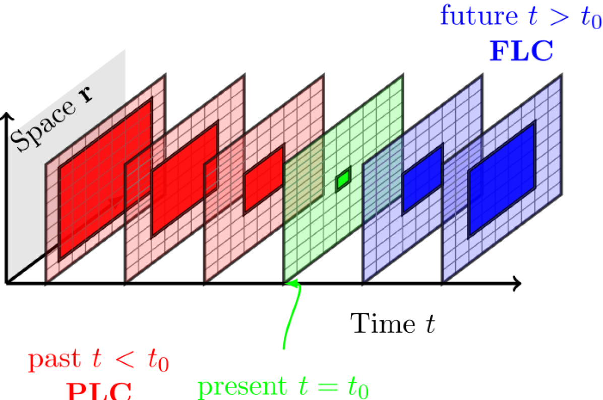
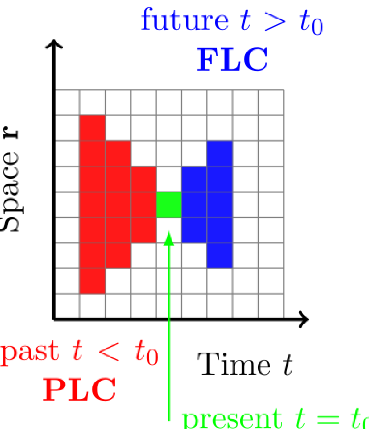
Analogously the future light cone (FLC) $L^{+}\left(\mathbf{r},t\right)$ is all future events which could be influenced by $\left(\mathbf{r},t\right)$. In practice, we limit PLCs and FLCs to finite horizons $h_{p}$ and $h_{f}$; together with $c$, these fix the dimensionality of light-cones; see Figure 1 for an illustration.

(a) $(1+1)D$ field

(b) $(2+1)D$ field

Figure 1: Geometry of past ( $\ell^{-}\left(\mathbf{r},t\right)$) and future ($\ell^{+}\left(\mathbf{r},t\right)$) light cones, with $h_{p}=3$, $h_{f}=2$, $c=1$.

For physically-plausible processes, then, we only have to find the conditional distribution of $X\left(\mathbf{r},t\right)$ given its PLC $\left(\ell^{-},\left(\mathbf{r},t\right)\right)$. Doing this for every $\left(\mathbf{r},t\right)$ in space-time, however, is still excessive. Not only do spatio-temporal patterns recur, but different histories can have similar predictive consequences. Thus we need not find $\mathbb{P}\left(X\left(\mathbf{r},t\right)\mid\left(\ell^{-},\left(\mathbf{r},t\right)\right)\right)$ for each $\left(\mathbf{r},t\right)$ separately, but can first summarize PLCs by predictively sufficient statistics, $\epsilon\left(\ell^{-},\left(\mathbf{r},t\right)\right)$, and then only find $\mathbb{P}\left(X\left(\mathbf{r},t\right)\mid\epsilon\left(\ell^{-},\left(\mathbf{r},t\right)\right)\right)$.

We now construct the minimal sufficient statistic, $\epsilon(\ell^{-}\left(\mathbf{r},t\right))$, following Shalizi (2003), to which we refer for some mathematical details, and references on predictive sufficiency.

Definition 2.1 (Equivalent configurations).

The past configurations $\ell_{i}^{-}$ at $\left(\mathbf{r},t\right)$ and $\ell_{j}^{-}$ at $\left(\mathbf{u},s\right)$ are predictively equivalent, $(\ell_{i}^{-},\left(\mathbf{r},t\right))\sim(\ell_{j}^{-},\left(\mathbf{u},s\right))$, if they have the same conditional distributions for FLCs, i.e.,

$$\mathbb{P}\left(L^{+}\left(\mathbf{r},t\right)\mid L^{-}\left(\mathbf{r},t\right)=\ell_{i}^{-}\right)=\mathbb{P}\left(L^{+}\left(\mathbf{u},s\right)\mid L^{-}\left(\mathbf{u},s\right)=\ell_{j}^{-}\right).$$

Let $\left[(\ell^{-},\left(\mathbf{r},t\right))\right]$ be the equivalence class of $(\ell^{-},\left(\mathbf{r},t\right))$, the set of all past configurations and coordinates that predict the same future as $\ell^{-}$ does at $\left(\mathbf{r},t\right)$. Let

$$\epsilon(\ell^{-},\left(\mathbf{r},t\right))\equiv\left[\ell^{-}\right].$$ (2)

be the function mapping each $(\ell^{-},\left(\mathbf{r},t\right))$ to its predictive equivalence class. The values $\epsilon$ can take are predictive states; they are the minimal statistics which are sufficient for predicting $L^{+}$ from $L^{-}$ (Shalizi, 2003).

Assumption 2.2 (Conditional invariance).

The predictive distribution of a PLC configuration $\ell^{-}$ does not change over time or space. That is, for all $\mathbf{r},t$, all $\mathbf{u},s$, and all past light-cone configurations $\ell^{-}$,

$$(\ell^{-},\left(\mathbf{r},t\right))\sim(\ell^{-},\left(\mathbf{u},s\right))$$ (3)

We may thus regard $\sim$ as an equivalence relation among PLC configurations, and $\epsilon$ as a function over $\ell^{-}$ alone.

Assumption 2.2 enables inference from a single realization of the process (as opposed to multiple independent realizations). For readability, we encode the space-time index $\left(\mathbf{r},t\right)$ by a single index $i=1,\ldots,N$.

The future is independent of the past given the predictive state (Shalizi, 2003),

$$\mathbb{P}\left(L^{+}_{i}\mid\ell^{-}_{i},\epsilon(\ell^{-}_{i})\right)=\mathbb{P}\left(L^{+}_{i}\mid\epsilon(\ell^{-}_{i})\right)$$ (4)

and, by construction,

$$\mathbb{P}\left(L^{+}_{i}\mid\ell^{-}_{i}\right)=\mathbb{P}\left(L^{+}_{i}\mid\epsilon(\ell^{-}_{i})\right).$$ (5)

Thus the prediction problem simplifies to estimating $\mathbb{P}\left(X_{i}\mid\epsilon(\ell^{-}_{i})\right)$ for each $i$.

2.2 A Statistical Predictive-States Model

The focus on predictive distributions in constructing the predictive states does not prevent us from using them to model the joint distribution.

Proposition 2.3.

The joint pdf of $X_{1},\ldots,X_{\tilde{N}}$ satisfies

$$\mathbb{P}\left(X_{1},\ldots,X_{\tilde{N}}\right)=\mathbb{P}\left(\mathbf{M}\right)\prod_{i=1}^{\tilde{N}}\mathbb{P}\left(X_{i}\mid\ell^{-}_{i}\right),$$ (6)

where $\mathbf{M}$ is the margin of the spatio-temporal process, i.e., all points in the field that do not have a completely observed PLC.

Proof.

See Supplementary Material, §A. ∎

Proposition 2.3 shows that the focus on conditional predictive distributions does not restrict the applicability of the light cone setup to forecasts alone, but is in fact a generative representation for any spatio-temporal process.

2.2.1 Minimal Sufficient Statistical Model

Given $\epsilon(\ell^{-}_{i})$ Eq. (6) simplifies to (omitting $\mathbb{P}\left(\mathbf{M}\right)$)

$$\mathbb{P}\left(X_{1},\ldots,X_{N}\mid\mathbf{M},\epsilon\right) =\prod_{i=1}^{N}\mathbb{P}\left(X_{i}\mid\ell_{i}^{-};\epsilon(\ell^{-}_{i})\right)$$

$$=\prod_{i=1}^{N}\mathbb{P}\left(X_{i}\mid\epsilon(\ell^{-}_{i})\right),$$ (7)

using (4). Any particular $\epsilon$ implicitly specifies the number of predictive states $K$, and all $K$ predictive distributions $\mathbb{P}\left(X_{i}\mid\epsilon(\ell^{-}_{i})\right)$. However, in practice only $X_{i}$ and $\ell^{-}_{i}$ are observed; the mapping $\epsilon$ is exactly what we are trying to estimate.

2.3 Predictive States as Hidden Variables

Since there is a one-to-one correspondence between the mapping $\epsilon$ and the set of equivalence classes / predictive states $\epsilon(\ell^{-})$ which are its range, Shalizi (2003) and Goerg and Shalizi (2012) do not formally distinguish between them. Here, however, it is important to keep distinction between the predictive state space $\mathcal{S}$ and the mapping $\epsilon:\ell^{-}_{i}\rightarrow\mathcal{S}$. Our EM algorithm is based on the idea that the predictive state is a hidden variable, $S_{i}$, taking values in the finite state space $\mathcal{S}=\{s_{1},\ldots,s_{K}\}$, and the mixture weights of PLC $\ell^{-}_{i}$ are the soft-threshold version of the mapping $\epsilon(\ell^{-}_{i})$. It is this hidden variable interpretation of predictive states that we use to estimate the minimal sufficient statistic $\epsilon$, the hidden state space $\mathcal{S}$, and the predictive distributions $\mathbb{P}\left(X_{i}\mid S_{i}=s_{j}\right)$.

Introducing the abbreviation $\mathbb{P}_{j}\left(\cdot\right)$ for $\mathbb{P}\left(\cdot\mid S_{i}=s_{j}\right)$, the latent variable approach lets (7) be written as

$$\prod_{i=1}^{N}\mathbb{P}\left(X_{i}\mid S_{i}\right)=\prod_{i=1}^{N}{\sum_{j=1}^{K}{\mathbf{1}\left(S_{i}=s_{j}\right)\mathbb{P}_{j}\left(X_{i}\right)}}.$$ (8)

Eq. (8) is the pdf of a $K$ component mixture model with complete data, and $\mathbf{1}\left(S_{i}=s_{j}\right)$ is a randomized version of $\epsilon:\ell^{-}_{i}\mapsto S_{i}$.

2.4 Log-likelihood of $\epsilon$

From (8) the complete data log-likelihood is, neglecting a $\log{\mathbb{P}\left(\mathbf{M}\right)}$ term,

$$\ell(\epsilon;\mathcal{D},S_{1}^{N}) =\sum_{i=1}^{N}\log\left(\sum_{j=1}^{K}\mathbf{1}\left(S_{i}=s_{j}\right)\mathbb{P}\left(X_{i}\mid\epsilon(\ell^{-}_{i})=s_{j}\right)\right)$$

$$=\sum_{i=1}^{N}\sum_{j=1}^{K}\mathbf{1}\left(S_{i}=s_{j}\right)\log\mathbb{P}\left(X_{i}\mid\epsilon(\ell^{-}_{i})=s_{j}\right),$$ (9)

where $S_{1}^{N}:=\{S_{1},\ldots,S_{N}\}$ and the second equality follows since $\mathbf{1}\left(S_{i}=s_{j}\right)=1$ for one and only one $j$, and $0$ otherwise.

The “parameters” in (9) are $\epsilon$ and $K$; $X_{i}$ and $\ell^{-}_{i}$ are observed, and $S_{i}$ is a hidden variable. The optimal mapping $\epsilon:L^{-}\rightarrow\mathcal{S}$ is the one that maximizes (9):

$$\epsilon^{*}=\operatorname*{arg\,max}_{\epsilon}{\ell(\epsilon;\mathcal{D},S_{i})}.$$ (10)

Without any constraints on $K$ or $\epsilon$ the maximum is obtained for $K=N$ and $\epsilon(\ell^{-}_{i})=\ell^{-}_{i}$; “the most faithful description of the data is the data”. As this tells us nothing about the underlying dynamics, we must put some constraints on $K$ and/or $\epsilon$ to get a useful solution. For now, assume that $K\ll N$ is fixed and we only have to estimate $\epsilon$; in Section 3.3, we will give a data-driven procedure to choose $K$.

2.5 Nonparametric Likelihood Approximation

To solve (10) with $K\ll N$ we need to evaluate (9) for candidate solutions $\epsilon$. We cannot do this directly, since (9) involves the unobserved $S_{i}$. Moreover, predictive distributions can have arbitrary shapes, so we want to use nonparametric methods, but this inhibits direct evaluation of the component distributions $\mathbb{P}\left(X_{i}\mid\epsilon(\ell^{-}_{i})=s_{j}\right)$.

We solve both difficulties together by using a nonparametric variant of the expectation-maximization (EM) algorithm (Dempster et al., 1977). Following the recent nonparametric EM literature (Hall et al., 2005; Benaglia et al., 2011; Bordes et al., 2007), we approximate the $\mathbb{P}\left(X_{i}\mid\epsilon(\ell^{-}_{i})=s_{j}\right)$ in the log-likelihood with kernel density estimators (KDEs) using a previous estimate $\widehat{\epsilon}^{(n)}$. That is we approximate (9) with $\widehat{\ell}^{(n)}(\epsilon;\mathcal{D},S_{i})$:

$$\sum_{i=1}^{N}{\sum_{j=1}^{K}{\mathbf{1}\left(S_{i}=s_{j}\right)\log\widehat{f}\left({X_{i}\mid\widehat{\epsilon}^{(n)}(\ell^{-}_{i})=s_{j}}\right)}},$$ (11)

where an equivalent version of $\widehat{f}\left({X_{i}\mid\widehat{\epsilon}^{(n)}(\ell^{-}_{i})=s_{j}}\right)$ is given below in (20).

3 EM Algorithm for Predictive State Space Assignment

Since $\epsilon$ maps to $\mathcal{S}$, the hidden state variable $S_{i}$ and the “parameter” $\epsilon$ play the same role. This in turn results in similar E and M steps. Figure 2 gives an overview of the proposed algorithm.

3.1 Expectation Step

The E-step requires the expected log-likelihood

$$Q(\epsilon\mid\epsilon^{(n)})=\mathbb{E}_{\mathcal{S}\mid\mathcal{D};\epsilon^{(n)}}\ell(\epsilon;\mathcal{D},S_{i}),$$ (12)

where expectation is taken with respect to $\mathbb{P}\left(S_{i}=s_{j}\mid\mathcal{D};\epsilon^{(n)}\right)$, the conditional distribution of the hidden variable $S_{i}$ given the data $\mathcal{D}$ and the current estimate $\epsilon^{(n)}$. Using (9) we obtain

$$\begin{split}Q(\epsilon\mid\epsilon^{(n)})=\sum_{i=1}^{N}\sum_{j=1}^{K}&\,\mathbb{P}\left(S_{i}=s_{j}\mid X_{i},\ell^{-}_{i};\epsilon^{(n)}(\ell^{-}_{i})\right)\\ &\times\log\mathbb{P}\left(X_{i}\mid\epsilon^{(n)}(\ell^{-}_{i})=s_{j}\right).\end{split}$$ (13)

As for $\ell(\epsilon;\mathcal{D})$ we use KDEs and obtain an approximate expected log-likelihood

$$\begin{split}\widehat{Q}^{(n)}(\epsilon\mid\epsilon^{(n)})=\sum_{i=1}^{N}\sum_{j=1}^{K}&\,\mathbb{P}\left(S_{i}=s_{j}\mid X_{i},\ell^{-}_{i};\epsilon^{(n)}(\ell^{-}_{i})\right)\\ &\times\log\widehat{f}\left(X_{i}\mid\widehat{\epsilon}^{(n)}(\ell^{-}_{i})=s_{j}\right)\end{split}$$ (14)

The conditional distribution of $S_{i}$ given its FLC and PLC, $\{X_{i},\ell^{-}_{i}\}$, comes from Bayes’ rule,

$$\mathbb{P}\left(S_{i}=s_{j}\mid X_{i},\ell^{-}_{i}\right) \propto\mathbb{P}\left(X_{i},\ell^{-}_{i}\mid S_{i}=s_{j}\right)\mathbb{P}\left(S_{i}=s_{j}\right)$$

$$=\mathbb{P}_{j}\left(X_{i}\right)\mathbb{P}_{j}\left(\ell^{-}_{i}\right)\mathbb{P}\left(S_{i}=s_{j}\right),$$ (15)

the second equality following from the conditional independence of $X_{i}$ and $\ell^{-}_{i}$ given the state $S_{i}$.

For brevity, let $w_{ij}:=\mathbb{P}\left(S_{i}=s_{j}\mid X_{i},\ell^{-}_{i}\right)$, an $N\times K$ weight matrix $\mathbf{W}$, whose rows are probability distributions over states. This $\mathbf{w}_{i}$ is the soft-thresholding version of $\epsilon(\ell^{-}_{i})$, so we can write the expected log-likelihood in terms of $\mathbf{W}$,

$$\widehat{Q}^{(n)}(\mathbf{W}\mid\widehat{\mathbf{W}}^{(n)}) =\sum_{i=1}^{N}\sum_{j=1}^{K}{w_{ij}\cdot\log\mathbb{P}\left(X_{i}\mid\widehat{\mathbf{W}}^{(n)}_{j}\right)}$$ (16)

The current $\widehat{\mathbf{W}}^{(n)}$ can be used to update (conditional) probabilities in (15) by

$$\widehat{w}_{ij}^{(n+1)}\propto \quad\widehat{f}(x_{i}\mid S_{i}=s_{j};\widehat{\mathbf{W}}^{(n)})$$ (17)

$$\times\mathcal{N}\left(\ell_{i}^{-}\mid\widehat{\boldsymbol{\mu}}_{j}^{(n)},\widehat{\boldsymbol{\Sigma}}_{j}^{(n)};\widehat{\mathbf{W}}^{(n)}\right)$$ (18)

$$\times\frac{\widehat{N}_{j}^{(n)}}{N},$$ (19)

where i) $\widehat{N}_{j}^{(n)}=\sum_{i=1}^{N}\widehat{\mathbf{W}}^{(n)}_{ij}$is the effective sample size of state $s_{j}$, ii) $\widehat{\boldsymbol{\mu}}_{j}^{(n)}$and $\widehat{\boldsymbol{\Sigma}}_{j}^{(n)}$ are weighted mean and covariance matrix estimators of the PLCs using the $j$th column of $\widehat{\mathbf{W}}^{(n)}$, and iii) the FLC distribution is estimated with a weighted KDE (wKDE) $$\widehat{f}(x\mid S=s_{j};\widehat{\mathbf{W}}^{(n)})=\frac{1}{\widehat{N}_{j}^{(n)}}\sum_{r=1}^{N}\widehat{\mathbf{W}}_{rj}^{(n)}K_{h_{j}}(\lVert x_{r}-x\rVert),$$ (20) Here the weights are again the $j$th column of $\widehat{\mathbf{W}}^{(n)}$, and $K_{h_{j}}$ is a kernel function with a state-dependent bandwidth $h_{j}$. We used a Gaussian kernel, and to get a good, cluster-adaptive bandwidth $h_{j}$, we pick out on those $x_{i}$ for which $\operatorname*{arg\,max}_{k}{w_{ik}}=j$ (hard-thresholding of weights; cf. Benaglia et al. 2011) and apply Silverman’s rule-of-thumb-bandwidth (bw.ndr0 in the R function density). After estimation, we normalize each $\widehat{\mathbf{w}}_{i}$ in (17), $\widehat{w}_{ij}^{(n+1)}\leftarrow\frac{\widehat{w}_{ij}^{(n+1)}}{\sum_{j=1}^{K}{\widehat{w}_{ij}^{(n+1)}}}$.

Ideally, we would use a non-parametric estimate for the PLC distribution, e.g., forest density estimators (Liu et al., 2011; Chow and Liu, 1968). Currently, however, such estimators are too slow to handle many iterations at large $N$, so we model state-conditional PLC distributions as multivariate Gaussians. Simulations suggest that this is often adequate in practice.

3.2 Approximate Maximization Step

In parametric problems, the M-step solves

$$\epsilon^{(n+1)}=\operatorname*{arg\,max}_{\epsilon}{\widehat{Q}^{(n)}(\epsilon\mid\epsilon^{(n)})},$$ (21)

to improve the estimate. Starting from a guess $\epsilon^{(0)}$, the EM algorithm iterates (12) and (21) to convergence.

In nonparametric problems, finding an $\epsilon^{(n+1)}$ that increases $\widehat{Q}^{(n)}(\epsilon\mid\epsilon^{(n)})$ is difficult, since wKDEs with non-zero bandwidth are not maximizing the likelihood; they are not even guaranteed to increase it. Optimizing (14) by brute force isn’t computationally feasible either, as it would mean searching $K^{N}$ state assignments (cf. Bordes et al. 2007).

0. Initialization: Set $n=0$. Split data $\mathcal{D}=\{X_{i},\ell_{i}^{-}\}_{i=1}^{N}$ in $\mathcal{D}_{train}$ and $\mathcal{D}_{test}$. Initialize states randomly from $\{s_{1},\ldots,s_{K}\}$ $\rightarrow$ Boolean $\widehat{\mathbf{W}}^{(0)}$. 1. E-step: Obtain updated $\widehat{\mathbf{W}}^{(n+1)}$ via (17). 2. Approximate M-step: Update mixture pdfs $\mathbb{P}\left(x_{i}\mid S_{i}=s_{j}\right)$ via (20) with $\widehat{\mathbf{W}}^{(n+1)}$. 3. Out-of-sample Prediction: Evaluate out-of-sample MSE for $\widehat{\mathbf{W}}^{(n+1)}$ by predicting FLCs from PLCs in $\mathcal{D}_{test}$. Set $n=n+1$. 4. Temporary convergence: Iterate 1 - 3 until $$\lVert\widehat{\mathbf{W}}^{(n)}-\widehat{\mathbf{W}}^{(n-1)}\rVert<\delta$$ (22) 5. Merging: Estimate pairwise distances (or test) $$\widehat{d}_{jk}=\operatorname{dist}\left(\widehat{f}^{(n)}_{j},\widehat{f}^{(n)}_{k}\right)\forall j,k=1,\ldots,K.$$ (23) (a) If $K>1$: determine $(j^{(\min)},k^{(\min)})=\operatorname*{arg\,min}_{j\neq k}\widehat{d}_{jk}$ and merge these columns $$\mathbf{W}^{(n)}_{j^{(\min)}}\leftarrow\mathbf{W}^{(n)}_{j^{(\min)}}+\mathbf{W}^{(n)}_{k^{(\min)}}$$ (24) Omit column $k^{(\min)}$ from $\mathbf{W}^{(n)}_{k^{(\min)}}$, set $K=K-1$, and re-start iterations at 1. (b) If $K=1$: return $\widehat{\mathbf{W}}^{*}$ with lowest out-of-sample MSE.

Figure 2: Mixed LICORS: nonparametric EM algorithm for predictive state recovery.

However, in our particular setting the parameter space and the expectation of the hidden variable coincide, since $\widehat{\mathbf{w}}_{i}$ is a soft-thresholding version of $\epsilon(\ell^{-}_{i})$. Furthermore, none of the estimates above requires a deterministic $\epsilon$ mapping; they are all weighted MLEs or KDEs. Thus, like Benaglia et al. (2009), we take the weights from the E-step, $\widehat{\mathbf{W}}^{(n+1)}$, to update each component distribution using (20). This in turn can then be plugged into (11) to update the likelihood function, and in (17) for the next E-step.

The wKDE update does not solve (21) nor does it provably increase the log-likelihood (although in simulations it often does so). We thus use cross-validation (CV) to select the best $\widehat{\mathbf{W}}^{*}$, and henceforth do not rely on an ever-increasing log-likelihood as the usual stopping rule in EM algorithms (see Section 5 for details).

3.3 Data-driven Choice of $K$: Merge States To Obtain Minimal Sufficiency

One advantage of the mixture model in (8) is that predictive states have, by definition, comparable conditional distributions. Since conditional densities can be tested for equality by a nonparametric two-sample test (or using a distribution metric), we can merge nearby classes. We thus propose a data-driven automatic selection of $K$, which solves this key challenge in fitting mixture models: 1) start with a sufficiently large number of clusters, $K_{\max}<N$; 2) test for equality of predictive distribution each time the EM reaches a (local) optimum; 3) merge until $K=1$ (iid case) – step 5 in Fig. 2; 4) choose the best model $\widehat{\mathbf{W}}^{*}$ (and thus $K^{*}$) by CV.

4 Forecasting Given New Data

The estimate $\widehat{\mathbf{W}}^{*}$ can be used to forecast $\tilde{X}$ given a new $\tilde{\ell}^{-}$. Integrating out $S_{i}$ yields a mixture

$$\mathbb{P}\left(\tilde{X}\mid\tilde{\ell}^{-}\right) =\sum_{j=1}^{K}\mathbb{P}\left(\tilde{S}=s_{j}\mid\tilde{\ell}^{-}\right)\cdot\mathbb{P}_{j}\left(\tilde{X}\right).$$ (25)

As $\mathbb{P}_{j}\left(\tilde{X}\right)=\mathbb{P}\left(\tilde{X}=x\mid\tilde{S}=s_{j}\right)$ is independent of $\tilde{\ell}^{-}$ we do not have to re-estimate them for each $\tilde{\ell}^{-}$, but can use the wKDEs in (20) from the training data.

The mixture weights $\tilde{w}_{j}:=\mathbb{P}\left(\tilde{S}=s_{j}\mid\tilde{\ell}^{-}\right)$ are in general different for each PLC and can again be estimated using Bayes’s rule (with the important difference that now we only condition on $\tilde{\ell}^{-}$, not on $\tilde{X}$):

$$\widehat{\mathbf{w}}_{j}(\tilde{\ell}^{-};\widehat{\mathbf{W}}^{*}) \propto\widehat{\mathbb{P}}\left(\tilde{\ell}^{-}\mid\tilde{S}=s_{j};\widehat{\mathbf{W}}^{*}\right)\times\widehat{\mathbb{P}}\left(\tilde{S}=s_{j};\widehat{\mathbf{W}}^{*}\right)$$

$$=\mathcal{N}\left(\tilde{\ell}^{-};\widehat{\boldsymbol{\mu}}_{(j)}^{*},\widehat{\boldsymbol{\Sigma}}_{(j)}^{*};\widehat{\mathbf{W}}^{*}\right)\times\frac{\widehat{N}_{j}^{*}}{N}.$$ (26)

After re-normalization of $\widehat{\tilde{\mathbf{w}}}=(\widehat{\tilde{w}}_{1}^{*},\ldots,\widehat{\tilde{w}}_{K}^{*})$, the predictive distribution (25) can be estimated via

$$\widehat{\mathbb{P}}\left(\tilde{X}=x\mid\tilde{\ell}^{-}\right) =\sum_{j=1}^{K}\widehat{\tilde{w}}_{j}^{*}\cdot\widehat{f}\left(\tilde{X}=x\mid S_{i}=s_{j};\widehat{\mathbf{W}}^{(*)}\right).$$ (27)

A point forecast can then be obtained by a weighted combination of point estimates in each component (e.g. weighted mean), or by the mode of the full distribution. In the simulations we use the weighted average from each component as the prediction of $\tilde{X}$.

5 Simulations

To evaluate the predictive ability of mixed LICORS in a practical, non-asymptotic context we use the following simulation. The continuous-valued $(1+1)D$ field $X\left(\mathbf{r},t\right)$ has a discrete latent state space $d\left(\mathbf{r},t\right)$. The observable field $X\left(\mathbf{r},t\right)$ evolves according to a conditional Gaussian distribution,

$$\mathbb{P}\left(X\left(\mathbf{r},t\right)\mid d\left(\mathbf{r},t\right)\right) =\begin{cases}\mathcal{N}(d\left(\mathbf{r},t\right),1),&\text{ if }|d\left(\mathbf{r},t\right)|<4,\\ \mathcal{N}(0,1),&\text{otherwise},\end{cases}$$ (28)

and initial conditions: $$X\left(\mathbf{\cdot},1\right)=X\left(\mathbf{\cdot},2\right)=\boldsymbol{0}\in\mathbb{R}^{|S|}.$$ (29)

The state space $d\left(\mathbf{r},t\right)$ evolves with the observable field,

$$\begin{split}d\left(\mathbf{r},t\right)=&\left[\frac{\sum_{i=-2}^{2}{X\left(\mathbf{(r+i)\bmod|S|},t-2\right)}}{5}\right.\\ &-\left.\frac{\sum_{i=-1}^{1}{X\left(\mathbf{(r+i)\bmod|S|},t-1\right)}}{3}\right]\end{split}$$ (30)

where $[x]$ is the closest integer to $x$. In words, Eq. (30) says that the latent state $d\left(\mathbf{r},t\right)$ is the rounded difference between the sample average of the $5$ nearest sites at $t-2$ and the sample average of the $3$ nearest sites at $t-1$. Thus $h_{p}=2$ and $c=1$.

If we include the present in the FLC, (28) gives $h_{f}=0$, making FLC distributions one-dimensional. As $d\left(\mathbf{r},t\right)$ is integer-valued and the conditional distribution becomes $\mathcal{N}(0,1)$ if $|d\left(\mathbf{r},t\right)|>4$, the system has $7$ predictive states, $\{s_{-3},s_{-2},\ldots,s_{2},s_{3}\}$, distinguished by the conditional mean $\mathbb{E}\left(X\left(\mathbf{r},t\right)\mid s_{k}\right)=k$. Thus $X\left(\mathbf{r},t\right)\mid s_{k}=\mathcal{N}(k,1)$, $k=-3,-2,\ldots,2,3$.

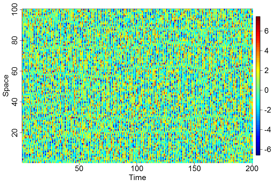
(a) observed field $X\left(\mathbf{r},t\right)$

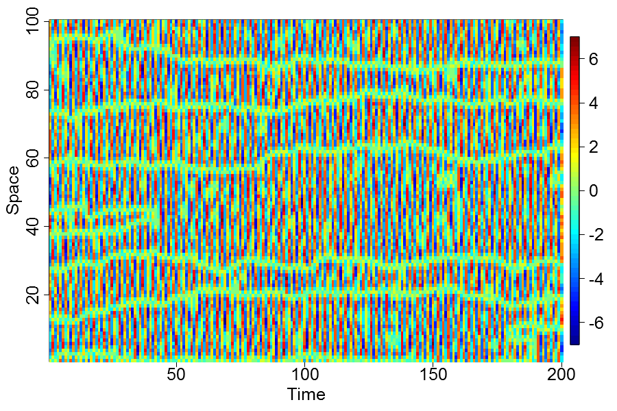
(b) state-space $d\left(\mathbf{r},t\right)$

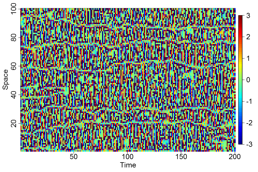
Figure 3: Simulation of (28) – (30).

Figure 4: Mixed LICORS with $h_{p}=2$ and $K_{\max}=15$ starting states. Nonparametric estimates of conditional predictive distributions $\mathbb{P}\left(X=x\mid S=s_{j}\right)$ (top-left); trace plots for log-likelihood and MSE (right).

Figure 3 shows one realization of (28) – (30) for $\mathbf{S}=\{1,\ldots,100\}$ (vertical) and $t=1,\ldots,T=200$ (left to right), where we discarded the first $100$ time steps as burn-in to avoid too much dependence on the initial conditions (29). While the (usually unobserved) state space has distinctive green temporal traces and also alternating red and blue patches, the observed field is too noisy to clearly see any of these patterns.

(a) estimated predictive states $\widehat{S}\left(\mathbf{r},t\right)$

(b) true predictive states $S\left(\mathbf{r},t\right)$

(c) residuals

Figure 5: Mixed LICORS model fit and residual check.

Figure 4 summarizes one run of mixed LICORS with $K=15$ initial states, $h_{p}=2$, and $L_{1}$ distance in (23). The first $100$ time steps were used as training data, and the second half as test data. The optimal $\widehat{\mathbf{W}}^{*}$, which minimized the out-of-sample weighted MSE, occurred at iteration $502$, with $\widehat{K}=9$ estimated predictive states. The trace plots show large temporary drops (increases) in the log-likelihood (MSE) whenever the EM reaches a local optimum and merges two states. After merging, the forecasting performance and log-likelihood quickly return to — or even surpass — previous optima.

The predictions from $\widehat{\mathbf{W}}^{*}$ in Fig. 5(a) show that mixed LICORS is practically unbiased – compare to the visually indistinguishable true state space in Fig. 5(b). The residuals in Fig. 5(c) show no obvious patterns except for a larger variance in the right half (training vs. test data).

5.1 Mixed versus Hard LICORS

Mixed LICORS does better than hard LICORS at forecasting. We use $100$ independent realizations of (28) – (30) and for each one we train the model on the first half, and test it on the second (future) half. Lower out-of-sample future MSEs are, of course, better.

We use EM as outlined in Fig. 2 with $K_{\max}=15$ states, $10^{3}$ maximum number of iterations. We keep the estimate $\widehat{\mathbf{W}}^{*}$ with the lowest out-of-sample MSE over $10$ independent runs. The first run is initialized with a K-means++ clustering (Arthur and Vassilvitskii, 2007) on the PLC space; state initializations in the remaining nine runs were uniformly at random from $\mathcal{S}=\{s_{1},\ldots,s_{15}\}$.

To test whether mixed LICORS accurately estimates the mapping $\epsilon:\ell^{-}\mapsto\mathcal{S}$, we also predict FLCs of an independently generated realization of the same process. If the out-of-sample MSE for the independent field is the same as the out-of-sample MSE for the future evolution of the training data, then mixed LICORS is not just memorizing fluctuations in any given realization, but estimates characteristics of the random field. We calculated both weighted-mixture forecasts, and the forecast of the state with the highest weight.

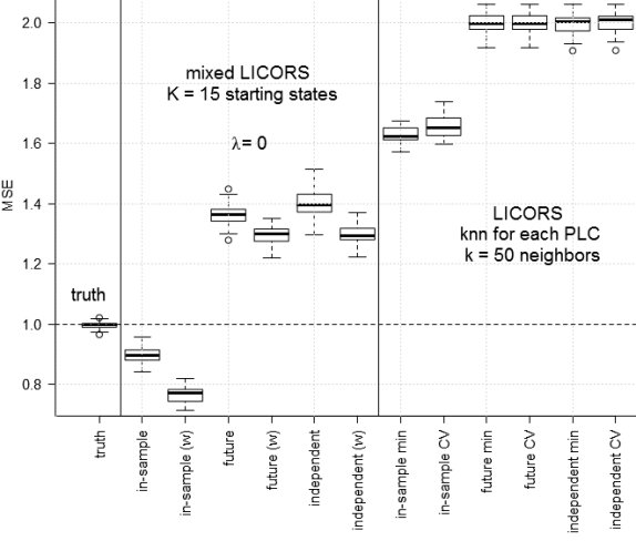
Figure 6: Comparing mixed and hard LICORS by forecast MSEs.

Figure 6 shows the results. Mixed LICORS greatly improves upon the hard LICORS estimates, with up to $34\%$ reduction in out-of-sample MSE. As with hard LICORS, the MSE for future and independent realizations are essentially the same, showing that mixed LICORS generalizes from one realization to the whole process. As the weights often already are $0$/$1$ assignments, weighted-mixture prediction is only slightly better than using the highest-weight state.

5.2 Simulating New Realizations of The Underlying System

Recall that all simulations use (29) as initial conditions. If we want to know the effect of different starting conditions, then we can simply use Eqs. (28) & (30) to simulate that process, since they fully specify the evolution of the stochastic process. In experimental studies, however, researchers usually lack such generative models; learning one is often the point of the experiment in the first place.

Since mixed LICORS estimates joint and conditional predictive distributions, and not only the conditional mean, it is possible to simulate a new realization from an estimated model. Figure 7 outlines this simulation procedure. We will now demonstrate that mixed LICORS can be used instead to simulate from different initial conditions without knowing Eqs. (28) & (30).

0. Initialize field $\{X\left(\mathbf{\cdot},1-\tau\right)\}_{\tau=1}^{h_{p}}$. Set $t=1$. 1. Fetch all PLCs at time $t$: $P_{t}=\{\ell^{-}\left(\mathbf{r},t\right)\}_{\mathbf{r}\in\mathbf{S}^{\operatorname{new}}}$ 2. For each $\ell^{-}\left(\mathbf{r},t\right)\in P_{t}$: (a) draw state $s_{j}\sim\mathbb{P}\left(S=s_{j}\mid\ell^{-}\left(\mathbf{r},t\right)\right)$ (b) draw $X\left(\mathbf{r},t\right)\sim\mathbb{P}\left(x\mid S=s_{j}\right)$ 3. If $t<t_{\max}$, set $t=t+1$ and go to step 1. Otherwise return simulation $\{X\left(\mathbf{\cdot},t\right)\}_{t=1}^{t_{\max}}$.

Figure 7: Simulate new realization from spatio-temporal process on $\mathbf{S}^{\operatorname{new}}\times\{1,\ldots,t_{\max}\}$ using true and estimated dynamics (use (4) in 2a; (20) in 2b).

(a) simulations from true dynamics

(b) simulations from estimated dynamics

Figure 8: Simulating another realization of (28) & (30) but with different starting conditions.

For example, Fig. 8(a) shows a simulation using the true mechanisms in (28) & (30) with starting conditions $X\left(\mathbf{\cdot},1\right)=-\boldsymbol{1}$ and $X\left(\mathbf{\cdot},2\right)=\pm\boldsymbol{3}\in\mathbb{R}^{|\mathbf{S}|}$ in alternating patches of ten times $3$, ten times $-3$, ten times $3$, etc. (total of $10$ patches since $|\mathbf{S}|=100$). The first couple of columns (on the left) are influenced by different starting conditions, but the initial effect dies out soon (since $h_{p}=2$) and similar structures (left to right traces) as in simulations with (29) emerge (Fig. 3).

Figure 8(b) shows simulations solely using the mixed LICORS estimates in Fig. 4. While the patterns are quantitatively different (due to random sampling), the qualitative structures are strikingly similar. Thus mixed LICORS can not only accurately estimate $S\left(\mathbf{r},t\right)$, but also learn the optimal prediction rule (28) solely from the observed data $X\left(\mathbf{r},t\right)$.

6 Discussion

Mixed LICORS attacks the problem of reconstructing the predictive state space of a spatio-temporal process through a nonparametric, EM-like algorithm, softly clustering observed histories by their predictive consequences. Mixed LICORS is a probabilistic generalization of hard LICORS and can thus be easily adapted to other statistical settings such as classification or regression. Simulations show that it greatly outperforms its hard-clustering predecessor.

However, like other state-of-the-art nonparametric EM-like algorithms (Hall et al., 2005; Bordes et al., 2007; Mallapragada et al., 2010), theoretical properties of our procedure are not yet well understood. In particular, the nonparametric estimation of mixture models poses identifiability problems (Benaglia et al., 2009, §2 and references therin). Here, we demonstrated that in practice mixed LICORS does not suffer from identifiability problems, and outperforms (identifiable) hard-clustering methods.

We also demonstrate that mixed LICORS can learn spatio-temporal dynamics from data, which can then be used for simulating new experiments, whether from the observed initial conditions or from new ones. Simulating from observed conditions allows for model checking; simulating from new ones makes predictions about unobserved behavior. Thus mixed LICORS can in principle make a lot of expensive, time- and labor-intensive experimental studies much more manageable and easier to plan. In particular, mixed LICORS can be applied to e.g., functional magnetic resonance imaging (fMRI) data to analyze and forecast complex, spatio-temporal brain activity. Due to space limits we refer to future work.

Acknowledgments

We thank Stacey Ackerman-Alexeeff, Dave Albers, Chris Genovese, Rob Haslinger, Martin Nilsson Jacobi, Heike Jänicke, Kristina Klinkner, Cristopher Moore, Jean-Baptiste Rouquier, Chad Schafer, Rafael Stern, and Chris Wiggins for valuable discussion, and Larry Wasserman for detailed suggestions that have improved all aspects of this work. GMG was supported by an NSF grant (# DMS 1207759). CRS was supported by grants from INET and from the NIH (# 2 R01 NS047493).

APPENDIX – SUPPLEMENTARY MATERIAL

Appendix A Proofs

Here we will show that the joint pdf of the entire field conditioned on its margin (Figure 9, gray area) equals the product of the predictive conditional distributions.

Proof of Proposition 2.3.

To simplify notation, we assign index numbers $i\in 1,\ldots N$ to the space-time grid $\left(\mathbf{s},t\right)$ to ensure that the PLC of $i_{1}$ cannot contain $X_{i_{2}}$ if $i_{2}>i_{1}$. We can do this by iterating through space and time in increasing order over time (and, for fixed $t$, any order over space):

$$\begin{split}\left(\mathbf{s},t\right),\mathbf{s}\in\mathbf{S},t\in\mathbb{T}&\rightarrow\left(i_{(t-1)\cdot|\mathbf{S}|+1},\ldots,i_{(t-1)\cdot|\mathbf{S}|+|\mathbf{S}|)}\right)\\ &=(t-1)\cdot|S|+(1,\ldots,{|S|}).\end{split}$$ (31)

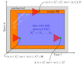
Figure 9: Margin of spatio-temporal field in $(1+1)D$.

We assume that the process we observed is part of a larger field on an extended grid $\tilde{\mathbf{S}}\times\tilde{\mathbb{T}}$, with $\tilde{\mathbf{S}}\supset\mathbf{S}$ and $\tilde{\mathbb{T}}=\{-(h_{p}-1),\ldots,0,1,\ldots T$, for a total of $\tilde{N}>N$ space-time points, $X_{1},\ldots,X_{\tilde{N}}$. The margin $\mathbf{M}$ are all points $X\left(\mathbf{s},u\right)$, $\left(\mathbf{s},u\right)\in\tilde{\mathbf{S}}\times\tilde{\mathbb{T}}$ that do not have a fully observed past light cone. Formally,

$$\mathbf{M}=\{X\left(\mathbf{s},u\right)\mid\ell^{-}\left(\mathbf{s},u\right)\notin\{X\left(\mathbf{r},t\right),\left(\mathbf{r},t\right)\in\mathbf{S}\times\mathbb{T}\}\},$$ (32)

The size of $\mathbf{M}$ depends on the past horizon $h_{p}$ as well as the speed of propagation $c$, $\mathbf{M}=\mathbf{M}\left(h_{p},c\right)$.

In Figure 9, the part of the field with fully observed PLCs are marked in red. Points in the margin, in gray, have PLCs extending into the fully unobserved region (blue). Points in the red area have a PLC that lies fully in the red or partially in the gray, but never in the blue area. As can be see in Fig. 9 the margin at each $t$ is a constant fraction of space, thus overall $\mathbf{M}$ grows linearly with $T$; it does not grow with an increasing $\mathbf{S}$, but stays constant.

For simplicity, assume that $X_{1},\ldots,X_{N}$ are from the truncated (red) field, such that all their PLCs are observed (they may lie in $\mathbf{M}$), and the remaining $\tilde{N}-N$ $X_{j}$s lie in $\mathbf{M}$ (with a PLC that is only partially unobserved). Furthermore let $X_{1}^{k}:=\{X_{1},\ldots,X_{k}\}$. Thus

$$\mathbb{P}\left(\{X\left(\mathbf{s},t\right)\mid\left(\mathbf{s},t\right)\in\tilde{\mathbf{S}}\times\tilde{\mathbb{T}}\}\right) =\mathbb{P}\left(X_{1}^{\tilde{N}}\right)$$

$$=\mathbb{P}\left(X_{1}^{N},\mathbf{M}\right)$$

$$=\mathbb{P}\left(X_{1}^{N}\mid\mathbf{M}\right)\mathbb{P}\left(\mathbf{M}\right)$$

The first term factorizes as

$$\mathbb{P}\left(X_{1}^{N}\mid\mathbf{M}\right)$$

$$=\mathbb{P}\left(X_{N}\mid X_{1}^{N-1},\mathbf{M}\right)\mathbb{P}\left(X_{1}^{N-1}\mid\mathbf{M}\right)$$

$$=\mathbb{P}\left(X_{N}\mid\ell^{-}_{N}\cup\{X_{1}^{N-1},\mathbf{M}\}\setminus\{\ell^{-}_{N}\}\right)\mathbb{P}\left(X_{1}^{N-1}\mid\mathbf{M}\right)$$

$$=\mathbb{P}\left(X_{N}\mid\ell^{-}_{N}\right)\mathbb{P}\left(X_{1}^{N-1}\mid\mathbf{M}\right)$$

where the second-to-last equality follows since by (31), $\ell^{-}_{N}\subset\{X_{k}\mid 1\leq k<N\}\cup\mathbf{M}$, and the last equality holds since $X_{i}$ is conditional independent of the rest given its own PLC (due to limits in information propagation over space-time).

By induction,

$$\mathbb{P}\left(X_{1},\ldots,X_{N}\mid\mathbf{M}\right) =\prod_{j=0}^{N-1}\mathbb{P}\left(X_{N-j}\mid\ell^{-}_{N-j}\right)$$ (33)

$$=\prod_{i=1}^{N}\mathbb{P}\left(X_{i}\mid\ell^{-}_{i}\right)$$ (34)

This shows that the conditional log-likelihood maximization we use for our estimators is equivalent (up to a constant) to full joint maximum likelihood estimation. ∎

Appendix B Predictive States and Mixture Models

Another way to understand predictive states is as the extremal distributions of an optimal mixture model (Lauritzen, 1974, 1984).

To predict any variable $L^{+}$, we have to know its distribution $\mathbb{P}\left(L^{+}\right)$. If, as often happens, that distribution is very complicated, we may try to decompose it into a mixture of simpler “base” or “extremal” distributions, $\mathbb{P}\left(L^{+}\mid\theta\right)$, with mixing weights $\pi(\theta)$,

$$\mathbb{P}\left(L^{+}\right)=\int{\pi(\theta)\mathbb{P}\left(L^{+}\mid\theta\right)d\theta}~{}.$$ (35)

The familiar Gaussian mixture model, for instance, makes the extremal distributions to be Gaussians (with $\theta$ indexing both expectations and variances), and makes the mixing weights $\pi(\theta)$ a combination of delta functions, so that $\mathbb{P}\left(L^{+}\right)$ becomes a weighted sum of finitely-many Gaussians.

The conditional predictive distribution of $L^{+}\mid\ell^{-}$ in (35) is a weighted average over the extremal conditional distributions $\mathbb{P}\left(L^{+}\mid\theta,\ell^{-}\right)$,

$$\mathbb{P}\left(L^{+}\mid\ell^{-}\right)=\int{\pi(\theta|\ell^{-})\mathbb{P}\left(L^{+}\mid\theta,\ell^{-}\right)d\theta}~{}$$ (36)

This only makes the forecasting problem harder, unless $\mathbb{P}\left(L^{+}\mid\theta,\ell^{-}\right)\pi(\theta\mid\ell^{-})=\mathbb{P}\left(L^{+}\mid\hat{\theta}(\ell^{-})\right)\delta(\theta-\hat{\theta}(\ell^{-}))$, that is, unless $\hat{\theta}(\ell^{-})$ is a predictively sufficient statistic for $L^{+}$. The most parsimonious mixture model is the one with the minimal sufficient statistic, $\theta=\epsilon(\ell^{-})$. This shows that predictive states are the best “parameters” in (35) for optimal forecasting. Using them,

$$\mathbb{P}\left(L^{+}\right) =\sum_{j=1}^{K}\mathbb{P}\left(\epsilon(\ell^{-})=s_{j}\right)\mathbb{P}\left(L^{+}\mid\epsilon(\ell^{-})=s_{j}\right)$$ (37)

$$=\sum_{j=1}^{K}{\pi_{j}(\ell^{-})\cdot\mathbb{P}_{j}\left(L^{+}\right)}~{},$$ (38)

where $\pi_{j}(\ell^{-})$ is the probability that the predictive state of $\ell^{-}$ is $s_{j}$, and $\mathbb{P}_{j}\left(L^{+}\right)=\mathbb{P}\left(L^{+}\mid S=s_{j}\right)$. Since each light cone has a unique predictive state,

$$\pi_{j}(\ell^{-})=\begin{cases}1,&\text{ if }\epsilon(\ell^{-})=s_{j},\\ 0&\text{ otherwise}.\end{cases}$$ (39)

Thus the predictive distribution given $\ell^{-}_{i}$ is just

$$\mathbb{P}\left(L^{+}\mid\ell^{-}_{i}\right) =\sum_{j=1}^{K}{\pi_{j}(\ell^{-}_{i})\cdot\mathbb{P}_{j}\left(L^{+}\right)}=\mathbb{P}_{\epsilon(\ell^{-}_{i})}\left(L^{+}\right).$$ (40)

Now the forecasting problem simplifies to mapping $\ell^{-}_{i}$ to its predictive state, $\epsilon(\ell^{-}_{i})=s_{j}$; the appropriate distribution-valued forecast is $p_{j}(L^{+})$, and point forecasts are derived from it as needed.

This mixture-model point of view highlights how prediction benefits from grouping points by their predictive consequences, rather than by spatial proximity (as a Gaussian mixture would do). For us, this means clustering past light-cone configurations according to the similarity of their predictive distributions, not according to (say) the Euclidean geometry. Mixed LICORS thus learns a new geometry for the system, which is optimized for forecasting.

References

• Arthur and Vassilvitskii (2007) D.ย Arthur and S.ย Vassilvitskii. k-means++: The advantages of careful seeding. In H.ย Gabow, editor, Proceedings of the 18th Annual ACM-SIAM Symposium on Discrete Algorithms [SODA07], pages 1027โ€“1035, Philadelphia, 2007. Society for Industrial and Applied Mathematics. URL http://www.stanford.edu/~darthur/kMeansPlusPlus.pdf.
• Benaglia etย al. (2009) T.ย Benaglia, D.ย Chauveau, and D.ย R. Hunter. An EM-like algorithm for semi- and non-parametric estimation in multivariate mixtures. Journal of Computational and Graphical Statistics, 18:505โ€“526, 2009. URL http://sites.stat.psu.edu/~dhunter/papers/mvm.pdf.
• Benaglia etย al. (2011) T.ย Benaglia, D.ย Chauveau, and D.ย R. Hunter. Bandwidth selection in an EM-like algorithm for nonparametric multivariate mixtures. In D.ย R. Hunter, D.ย S.ย P. Richards, and J.ย L. Rosenberger, editors, Nonparametric Statistics and Mixture Models: A Festschrift in Honor of Thomas P. Hettmansperger. World Scientific, Singapore, 2011. URL http://hal.archives-ouvertes.fr/docs/00/35/32/97/PDF/npEM_bandwidth.pdf.
• Bordes etย al. (2007) L.ย Bordes, D.ย Chauveau, and P.ย Vandekerkhove. A stochastic EM algorithm for a semiparametric mixture model. Computational Statistics and Data Analysis, 51:5429โ€“5443, 2007. doi: 10.1016/j.csda.2006.08.015.
• Chow and Liu (1968) C.ย K. Chow and C.ย N. Liu. Approximating discrete probability distributions with dependence trees. IEEE Transactions on Information Theory, IT-14:462โ€“467, 1968.
• Dempster etย al. (1977) A.ย P. Dempster, N.ย M. Laird, and D.ย B. Rubin. Maximum likelihood from incomplete data via the EM algorithm. Journal of the Royal Statistical Society B, 39:1โ€“38, 1977. URL http://www.jstor.org/pss/2984875.
• Goerg and Shalizi (2012) G.ย M. Goerg and C.ย R. Shalizi. LICORS: Light cone reconstruction of states for non-parametric forecasting of spatio-temporal systems. Technical report, Department of Statistics, Carnegie Mellon University, 2012. URL http://arxiv.org/abs/1206.2398.
• Hall etย al. (2005) P.ย Hall, A.ย Neeman, R.ย Pakyari, and R.ย Elmore. Nonparametric inference in multivariate mixtures. Biometrika, 92:667โ€“678, 2005.
• Lauritzen (1974) S.ย L. Lauritzen. Sufficiency, prediction and extreme models. Scandinavian Journal of Statistics, 1:128โ€“134, 1974. URL http://www.jstor.org/pss/4615564.
• Lauritzen (1984) S.ย L. Lauritzen. Extreme point models in statistics. Scandinavian Journal of Statistics, 11:65โ€“91, 1984. URL http://www.jstor.org/pss/4615945. With discussion and response.
• Liu etย al. (2011) H.ย Liu, M.ย Xu, H.ย Gu, A.ย Gupta, J.ย Lafferty, and L.ย Wasserman. Forest density estimation. Journal of Machine Learning Research, 12:907โ€“951, 2011. URL http://jmlr.csail.mit.edu/papers/v12/liu11a.html.
• Lloyd (1982) S.ย Lloyd. Least squares quantization in PCM. Information Theory, IEEE Transactions on, 28(2):129 โ€“ 137, 1982. ISSN 0018-9448. doi: 10.1109/TIT.1982.1056489.
• Mallapragada etย al. (2010) P.ย K. Mallapragada, R.ย Jin, and A.ย K. Jain. Non-parametric mixture models for clustering. In E.ย R. Hancock, R.ย C. Wilson, T.ย Windeatt, I.ย Ulusoy, and F.ย Escolano, editors, Structural, Syntactic, and Statistical Pattern Recognition [SSPR//SPR 2010], pages 334โ€“343, New York, 2010. Springer-Verlag. doi: 10.1007/978-3-642-14980-1ห™32.
• R Development Core Team (2010) R Development Core Team. R: A Language and Environment for Statistical Computing. R Foundation for Statistical Computing, Vienna, Austria, 2010. URL http://www.R-project.org/. ISBN 3-900051-07-0.
• Shalizi (2003) C.ย R. Shalizi. Optimal nonlinear prediction of random fields on networks. Discrete Mathematics and Theoretical Computer Science, AB(DMCS):11โ€“30, 2003. URL http://arxiv.org/abs/math.PR/0305160.
APPENDIX โ€“ SUPPLEMENTARY MATERIAL