DO-TH 12/22
-Flavor Anatomy of Non-Leptonic Charm Decays
Abstract
We perform a comprehensive -flavor analysis of charmed mesons decaying to two pseudoscalar -octet mesons. Taking into account -breaking effects induced by the splitting of the quark masses, , we find that existing data can be described by -breaking of the order . The requisite penguin enhancement to accommodate all data on CP violation tends to be even larger than the one extracted from alone, strengthening explanations beyond the standard model. Despite the large number of matrix elements, correlations between CP asymmetries allow potentially to differentiate between different scenarios for the underlying dynamics, as well as between the standard model and various extensions characterized by symmetry and its subgroups. We investigate how improved measurements of the direct CP asymmetries in singly-Cabibbo-suppressed decays can further substantiate the interpretation of the data. We show that particularly informative are the asymmetries in versus , versus , , , and .
I Introduction
The recent measurements of direct CP violation in non-leptonic charm decays Aaij:2011in ; Collaboration:2012qw ; ICHEP12:Ko have been among the most exciting results in flavor physics in recent years. The combined significance of CP violation in charm decays is Amhis:2012bh ,
| (1) | |||||
where
| (2) |
for a decay of a meson, where denotes the weak decay amplitude of the flavor eigenstates. This measurement, together with the plethora of available charm data, makes an -flavor symmetry analysis worthwhile, aiming at an understanding within or beyond the standard model (SM). The basics of such an analysis were laid out some time ago Kingsley:1975fe ; Einhorn:1975fw ; Altarelli:1974sc ; Voloshin:1975yx ; Quigg:1979ic ; however, the present situation allows for a much more complete analysis than was possible before.
The symmetry is known to be broken rather severely in charm decays, the most striking example given by . However, as first pointed out in Savage:1991wu , this does not necessarily imply breaking on the amplitude level beyond the expected order of (see also Chau:1991gx for a similar analysis in the diagrammatic approach). Indeed, for a subset of decays it has been shown again recently that “nominal” breaking is sufficient to explain this ratio Pirtskhalava:2011va ; Feldmann:2012js ; Brod:2012ud .
Here we address the following questions:
-
i
How large is the requisite breaking in charm decays?
-
ii
How large is the requisite penguin, i.e., triplet matrix element enhancement to explain the observed CP violation?
-
iii
Can we distinguish between new physics (NP) contributing to operators in different representations of ? Which measurements would be particularly useful?
In our analysis we take into account -breaking induced by the splitting in the quark masses to first order; we compare our findings to the most complete, relevant data set of decays into two octet pseudoscalars and employ no further dynamical assumptions, the combination of which is where we go beyond previous works on SM CP violation, e.g., recently Brod:2011re ; Pirtskhalava:2011va ; Cheng:2012wr ; Bhattacharya:2012ah ; Feldmann:2012js ; Li:2012cfa ; Franco:2012ck ; Brod:2012ud , besides a detailed assessment of the -flavor anatomy of non-leptonic charm decays.
The plan of the paper is as follows: The -structure of hadronic two-body charm decays is given in Section II. In Section III we present fits to the data assuming the SM. In particular, all CP violation is induced by the Cabibbo-Kobayashi-Maskawa (CKM) mixing matrix. This analysis hence holds more generally in all models with this minimally flavor violating (MFV)-feature. In Section IV we allow for CP violation from NP characterized by different representations. We identify patterns in observables that can guide towards an identification of the underlying flavor dynamics. We conclude in Section V. In several appendices we give Clebsch-Gordan tables and subsidiary information.
II -decomposition
We present the -decomposition of various two-body charm decay amplitudes. The requisite Clebsch-Gordan coefficients are obtained using the tables and the program from Refs. de Swart:1963gc ; Kaeding:1995vq ; Kaeding:1995re .
II.1 -limit
-flavor symmetry allows to express the amplitudes of the various decays in terms of reduced matrix elements as
| (3) | |||||
where
| (4) |
We employ the commonly used classification for non-leptonic two-body charm decays according to the CKM hierarchy of their decay amplitudes: Cabibbo-favored (CF) at order one, singly-Cabibbo-suppressed (SCS) at order and doubly-Cabibbo-suppressed (DCS) at order in the Wolfenstein expansion, where .
In Eq. (3) label the representation of the final state and the interaction Hamiltonian, respectively. The relevant tensor product of the latter is written as
| (5) |
The initial -meson () is an anti-triplet. The two pseudoscalar octets in the final state can be decomposed as , where we symmetrized to account for Bose statistics and removed the dependence on the order of the final state mesons. The resulting coefficients are given in Table 1, where we introduced , which characterizes the CKM suppression of direct CP violation in decays. Note furthermore that we combined the coefficients of the and , as they have identical quantum numbers and therefore enter each amplitude with identical relative weight. Our findings are in agreement with Ref. Quigg:1979ic ; we disagree with a recent calculation Pirtskhalava:2011va in the sign of the amplitude111The authors of Ref. Pirtskhalava:2011va informed us that they agree with our expressions. The apparent sign differences are due to typos in their coefficient tables. . The inclusion of decays into pseudoscalar singlets is left for future work hjs13 .
| Decay | |||||
|---|---|---|---|---|---|
| SCS | |||||
| CF | |||||
| DCS | |||||
II.2 Breaking
Including -breaking through , i.e., leaving isospin symmetry intact, leads to breaking by a single representation , see also Savage:1991wu ; Hinchliffe:1995hz ; Pirtskhalava:2011va . The effective Hamiltonian contains at lowest order in the breaking the following decompositions:
| (6) | |||||
We consider the CKM-leading terms in the flavor-breaking only222One should revisit this assumption once CP data become more precise., hence the does not contribute. A notable exception is the decay , where the omission of would induce a spurious CP asymmetry. However, in the absence of new isospin violating interactions, the latter vanishes, see, e.g., Buccella:1992sg ; Grossman:2012eb . Furthermore, there are no non-zero matrix elements with the . The decay amplitudes can then be written as
| (7) |
where the denote the flavor-breaking contributions. We express them in terms of reduced matrix elements ,
| (8) | |||||
| (9) | |||||
| (10) |
analogous to Eq. (3).
Our findings for the coefficients are given in Table 4. We confirm the results given in Ref. Pirtskhalava:2011va except for the sign of the -terms in the -breaking part of the amplitude and the overall sign of the amplitude333See footnote 1..
For , the flavor structure of Eq. (II.2) leads to 15 -breaking matrix elements in addition to the three from the -limit. However, the coefficient matrix of Clebsch-Gordan coefficients does not have full rank, implying that not all matrix elements are physical. Since in fact the coefficient matrix has rank 11, we go on and reduce the number of matrix elements by 7. Specifically, the two representations have again the same quantum numbers, allowing us to combine the corresponding coefficients. Using Gaussian elimination we can further remove , , , , and . We do not mix leading elements in the process, and keep their normalizations when subleading matrix elements are absorbed. The -suppressed -breaking matrix elements that appear in the course of the redefinitions are again neglected as they are of higher order in the power counting employed in this work. Due to the reparametrizations, the sub- and superscripts on the cease to correspond to the -representations of the interaction and the final states. The appearing combinations have been normalized according to , in order not to change the relative normalization of the matrix elements. The resulting coefficients of the physical decomposition are given in Table 5. As anticipated, we end up with in total 13 independent matrix elements. In the following analyses we use Eqs. (8)-(10) with the coefficients from Table 5.
II.3 -breaking resistent sum rules
For the SCS 811 submatrix of Clebsch-Gordan coefficients including breaking in the physical parametrization has rank 7. Therefore, we know a priori that there is only one linear sum rule among the SCS amplitudes that remains valid after breaking. This sum rule is the well-known isospin relation Kwong:1993ri 444The apparent discrepancy between Eq. (11) and previous works Quigg:1979ic ; Kwong:1993ri is due to the different conventions used, specifically and .
| (11) |
One may ask whether there are also approximate sum rules which are broken by a single matrix element only. By calculating the rank of the corresponding matrices of Clebsch-Gordan coefficients, we find that among the SCS decays there is exactly one such sum rule. It is given by the (quasi-)triangle relation
| (12) |
which generalizes Ref. Kwong:1993ri , where breaking by triplet matrix elements only was considered. Setting the sides of the triangle have to obey , i.e., the longest of the three sides has to be smaller than the sum of the other two. This relation, if broken, would prove the necessity for ; it is, however, fulfilled by the data, given in Table 2. In the system before reparametrizations the right-hand side of Eq. (12) involves two matrix elements, and , and there is no sum rule with just one breaking matrix element.
In case the matrix element can be neglected and assuming MFV/SM, Eq. (12) allows to extract the size of the penguin contributions by measuring the involved branching ratios and CP-asymmetries by the usual triangle construction. It involves a common base for the triangle and its CP-conjugate one; the requisite weak phase can be taken from global CKM fits. A finite induces a correction to this procedure of the order of the -breaking, which however, is not so small.
Note that once CF and DCS modes are considered as well, further sum rules arise, see Brod:2012ud .
III SM/MFV Fits
We confront the -analysis from the previous section to data. The relevant measurements are compiled in Table 2. The fits are carried out using the augmented lagrangian conn1991globally ; birgin2008improving and Sbplx/Subplex algorithms Rowan1990 ; NLopt that are implemented in the “NLopt” code NLopt .
Our goal is to see whether gives a reasonable expansion for the full set of two-body decays of charm to pseudoscalar octet mesons, as shown possible for Savage:1991wu ; Pirtskhalava:2011va ; Feldmann:2012js ; Brod:2012ud . Our framework is MFV, which includes the SM. In these models CP violation is suppressed by , the relative weak phase is order one, .
To obtain the sizable CP violation observed in SCS decays, the triplet matrix elements, or , need to be sufficiently large, as they are the only ones not severely restricted by the branching ratio data. In terms of the low energy effective theory, this concerns penguin contractions of tree operators, the chromomagnetic dipole operator , where denotes the gluon field strength tensor, and the QCD penguins , all of which are purely triplets; we neglect the contributions from electroweak penguin operators. On the other hand, matrix elements involving the and representations receive contributions from the CKM-leading tree operators only.
Given the lack of a dynamical theory for hadronic charm decays, we have to resort to order-of-magnitude arguments when judging the fit results. The penguins (triplet matrix elements) are generically expected to be suppressed by a factor of compared to their tree counterparts. While this estimate cannot be expected to hold literally, in the past an upper bound of one for this ratio was widely considered conservative, leading to rather strong upper limits for SM CP violation. Possible enhancements have been discussed from an early stage on Abbott:1979fw ; Golden:1989qx , and recently, e.g., in Brod:2012ud ; Franco:2012ck . Note that the widely used analogy to the rule in kaon decays seems questionable, as the effect is expected to scale as Abbott:1979fw . However, enhancements, e.g., from rescattering cannot be excluded, but the necessary size for reaching the present central value seems a stretch, even in these analyses. Below, we introduce measures to quantify penguin enhancement for our analysis, and discuss the results obtained with present data.
III.1 Observables vs. degrees of freedom
The branching ratio of a decay into two pseudoscalars in terms of its amplitude is given as
| (13) |
with the phase space and normalization factor
| (14) |
We take the lifetimes and masses of the involved mesons from Beringer:1900zz .
For decays involving or , the direct CP asymmetry defined in Eq. (2) is not measured directly in the experiment. The corresponding indirect contributions are subtracted before fitting, see Appendix A for details.
We further employ differences and sums of direct CP asymmetries of SCS decays to final states , defined as
| (15) | |||
| (16) |
respectively. Considering instead of the individual asymmetries is experimentally advantageous; furthermore, to a very good accuracy, indirect contributions cancel in the difference.
We consider now the parameter budget of the ansatz including breaking effects at leading order versus the available experimental data. The 17 decay modes correspond in principle to 26 observables, i.e., 17 branching ratios, 8 (direct) CP asymmetries of SCS decays, and the strong phase difference between and . Since, however, the branching ratio is not measured yet, we are left with 25 observables.
On the parameter side within MFV/SM, there are three -limit matrix elements that come with a factor of and two -limit matrix elements that come with a factor of only. Of the five resulting matrix elements one can be chosen real as we are only sensitive to differences of strong phases. In the -limit there are hence nine real parameters. Taking into account -breaking, we end up with 13 independent matrix elements, see Section II.2, i.e., 25 real parameters.
III.2 The fate of unbroken
The need for flavor-breaking in SCS decays is most obvious in the large difference in the rates of the and modes, and in the enhanced branching ratio for , whose contribution vanishes in the limit. Fitting in this limit CF and DCS modes only also returns a very large , indicating sizable flavor breaking in these modes as well. This is seen, e.g., in .
Fits in unbroken using CF modes alone are not possible without additional assumptions, as the respective decay amplitudes have too much of a linear dependence, see also the observations made in Falk:2001hx . One may entertain the possibility of a CF-only fit by including -singlets in the final states. While this leads to additional observables and constraints, it also leads to additional matrix elements. The fit presented in Ref. Bhattacharya:2009ps yields for 1 degree of freedom () at the price of an additional dynamical assumption, which effectively relates matrix elements involving singlets and octets.
III.3 Fitting flavor-breaking
Including linear -breaking, we generically obtain good fits for a multitude of configurations. We find that a reasonable requires at least two -breaking matrix elements present. However, a fit with the assumption of triplet enhancement, as proposed in Abbott:1979fw ; Kwong:1993ri , and recently investigated in Pirtskhalava:2011va , does not yield acceptable results (), as no breaking enters the CF/DCS sector, see Table 5. Therefore, at least one matrix element other than is needed to describe the data; using, for instance, and we obtain . Note that a fit with to the SCS modes alone does work, .
To evaluate the convergence of the -expansion, we quantify the size of the flavor-breaking with the following measures: The size of the -breaking matrix elements, defined as
| (17) |
and the size of the -breaking amplitude, written as
| (18) |
To avoid a bias in the latter definition, we exclude the decay for which the amplitude in the limit is . We use both measures, as ignores the possibility of a suppression of -breaking from Clebsch-Gordan coefficients, while ignores the possibility of large cancellations.
We find that the data can be described by an -expansion with , see Fig. 1, where we show 68% (dark red) and 95% (light orange) confidence level (C.L.) contours relative to the best fit point, see Section III.4.
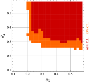
While solutions with larger breaking are not excluded by the data, we take this result as confirmation that the expansion works as good as could be expected. We therefore assume its validity in the following, and exclude solutions with cancellations by imposing in most fits.
Having established that with the current data the -expansion can be applied, we study the anatomy of the fit solutions. With the upper bound on , we obtain a fairly good fit to the full data set with for the configuration mentioned above, which consists of only the two matrix elements and . We stress that the minimal number of is two. A nicer fit, however, is obtained if at least three flavor-breaking matrix elements are present. Such examples are the configurations with , , or , , , both of which give . In the following we do not look at specific configurations with a minimal number of flavor breaking matrix elements but rather fit the full system with all .
| Observable | Measurement | References |
| SCS CP asymmetries | ||
| Amhis:2012bh ; Aubert:2007if ; Aaij:2011in ; Staric:2008rx ; Collaboration:2012qw ; ICHEP12:Ko | ||
| †ICHEP12:Ko ; Aubert:2007if ; Aaij:2011in ; Aaltonen:2011se ; Collaboration:2012qw | ||
| Bonvicini:2000qm | ||
| Bonvicini:2000qm | ||
| Mendez:2009aa | ||
| CKM12:Ko ; Cenci:2012uy ; Mendez:2009aa ; Link:2001zj | ||
| †Cenci:2012uy ; Ko:2010ng ; Mendez:2009aa | ||
| Mendez:2009aa | ||
| Indirect CP Violation | ||
| Amhis:2012bh | ||
| Beringer:1900zz | ||
| strong phase difference | ||
| ‡Amhis:2012bh | ||
| SCS branching ratios | ||
| Beringer:1900zz | ||
| Beringer:1900zz | ||
| Beringer:1900zz | ||
| Beringer:1900zz | ||
| Beringer:1900zz | ||
| Beringer:1900zz | ||
| Beringer:1900zz | ||
| Beringer:1900zz | ||
| CF∗ branching ratios | ||
| Beringer:1900zz | ||
| Beringer:1900zz | ||
| Beringer:1900zz | ||
| Beringer:1900zz | ||
| Beringer:1900zz | ||
| †Beringer:1900zz ; ICHEP12:Wang | ||
| DCS branching ratios | ||
| Beringer:1900zz | ||
| Beringer:1900zz | ||
III.4 Penguin enhancement
Next we turn to analyze the penguin enhancement. One possible definition is the following ratio:
| (19) |
In order to inspect also here the possibility of cancellations, we further define the penguin-to-tree fraction of a specific decay as
| (20) |
and its maximum
| (21) |
Here, for the same reason as in the case of , the decay is not taken into account.
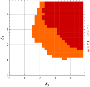
At the best fit point we obtain for 25 real fit parameters and an equal number of observables, obtained without a constraint on . The residual is caused by , which is measured nonzero at , but impossible to accommodate in the SM as it vanishes therein. We observe that is driven to huge values of in the fit. The reason for this strong enhancement lies not so much in the measurement for , but is due to the CP asymmetries , , and , which presently have very large central values, see Table 2. Their uncertainties are very large as well, rendering the effect insignificant for each single measurement. Together however, while still allowing for solutions with at C.L., they shift the C.L. region to very large values. Numerically, we obtain for , and for , in both cases saturating the bound. The latter value is slightly increased to when additionally imposing , indicating a very small correlation between the two measures. These observations are illustrated in Figs. 2 and 3. In the latter we show the influence of the largish measured CP asymmetries explicitly by excluding them from the fit. As a result, values of become allowed at C.L., consistent with Refs. Isidori:2011qw ; Feldmann:2012js ; Brod:2012ud , where these asymmetries have not been taken into account either.
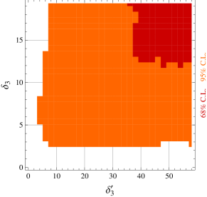
Closer inspection exhibits common features among the presented fits: The penguin matrix elements tend to be largely enhanced; there are large hierarchies between , depending on whether both triplet matrix elements and are present, as is the case in the decays , and , or not. In the latter modes indeed cancellations take place, yielding a smaller penguin amplitude with , and typically .
The maximum value of , on the other hand, usually comes from the decays where only is present, i.e., , or . Since furthermore typically , and the ratio of the Clebsch-Gordan coefficients of and in the latter modes equals , we understand why generically .
Taking into account the full dataset, we therefore find indications of even stronger enhanced penguin amplitudes than previous analyses relying on only. On the other hand, given the present uncertainties, the large central values responsible for this additional enhancement might be assigned to experimental fluctuations. As the enhancement indicated by is already very difficult to explain within the SM, any additional enhancement challenges this option further, making more precise measurements of the corresponding CP asymmetries extremely important.
IV Patterns of New Physics
In the absence of a dynamical theory or further input we still cannot make a definite statement on whether the enhanced penguins observed in Section III stem from physics within or beyond the SM. Note that knowing the weak phase precisely in MFV/SM is of no help as there is an approximate parametrization invariance: because of the smallness of , the rate measurements are not sensitive to the terms . The CP asymmetries are proportional to , however, they always involve unknown matrix elements not constrained by the rates. As a result, a shift in (e.g., a different weak phase) can in the fit always be absorbed by a shift in the magnitude of the respective matrix elements, as long as extreme values are avoided. Therefore, we set in the following , even when the NP model does not require a specific value. The potential enhancement factors from the Wilson coefficients are then identified by enhanced NP matrix elements, where we assume the absence of very large enhancement factors from QCD. Furthermore, we assume the validity of the expansion, using again the upper limit .
To investigate the interplay of NP and breaking, we study the following -limit relations involving CP asymmetries:
| (22) | ||||
| (23) | ||||
| (24) | ||||
| (25) |
The first three relations follow in the -spin limit, while the last one is an isospin relation. All relations can be obtained by inspecting, for instance, Table 1. Eqs. (22) and (23) can be rewritten as
| (26) | ||||
| (27) |
with corrections of the order , which are completely negligible compared to -breaking corrections. In addition, the -breaking representations and do not yield corrections to these relations, either.
The -expansion allows to quantify corrections to the above relations. Further deviations then indicate the presence of - and isospin changing interactions beyond the SM, models of which are discussed in the next section.
IV.1 New physics scenarios
We recall the -limit Hamiltonian for SCS decays within MFV/SM:
| (28) |
and involving the representations and , which, however, do not contribute significantly due to our assumption of “well-behaved” hadronic matrix elements, and are therefore neglected in the following. Here and in the following the subscript to the representation labels the shift in total isospin .
We discuss scenarios , which can be classified according to the contributing -representations. We use .
Very similar to the SM/MFV are models based on new physics in the alone (“triplet model”),
| (29) |
At the quark level, the corresponding operators are the chromomagnetic dipole operator and the QCD penguin operators. They have been discussed in supersymmetric Grossman:2006jg ; Giudice:2012qq ; Hiller:2012wf and extradimensional models DaRold:2012sz in the context of CP violation in charm.
We further consider a interaction
| (30) |
which arises from an operator with flavor structure (“HN model”). Those have been investigated recently in a peculiar variant of a 2-Higgs doublet model (2HDM) that links the top sector to charm Hochberg:2011ru . While the flavor structure is identical to the corresponding SM tree operator, it can have a different Dirac structure. As a result, the matrix elements of the -representation are independent of those appearing with a coefficient , and therefore not constrained by the data on the rates.
Finally, we allow for terms (“ model”),
| (31) |
The corresponding operators have flavor content . This structure may arise from tree level scalar exchanges as in 2HDMs or a color octet, see Altmannshofer:2012ur for a list. The appearance of a third representation carrying a weak phase different from the leading contributions implies significantly less correlation between different CP violating observables. This makes this scenario especially difficult to identify in patterns.
All models contribute to SCS decays only. We do not consider potential constraints on the scenarios with NP from 4-Fermi operators by mixing and Isidori:2011qw .
As QCD preserves -flavor, the irreducible representations form subsets which renormalize only among themselves Golden:1989qx . While such effects often have numerical relevance, they do not for our analysis, as we fit matrix elements rather then calculating them. We still ask whether the -anatomy of the NP models considered is radiatively stable.
A NP contribution in the does not “spread out” by mixing onto other representations. The situation for the scalar operators is likewise simple: They mix, together with their scalar and tensor color-flipped partners with the same flavor content at leading order only among themselves. The mixing onto the dipole operators vanishes for Buras:2000if ; Altmannshofer:2012ur . The total contribution to the amplitude therefore remains .
The scalar mixes among itself, color-flipped partners and onto chirality-flipped QCD-penguins; hence, renormalization group (RG) running modifies the weight between the and the set at the NP scale by Clebsch-Gordan coefficients. However, an explicit calculation of the leading order running between the weak and the charm scale shows that this effect is , and can be safely neglected for the purpose of our analysis. Anomalous dimensions can be taken from, e.g., Hiller:2003js .
The RG stability depends in general on the Dirac structure. We use in the following the corresponding -classifications, but have in mind the model examples where RG effects can be neglected.
IV.2 Patterns
In this section we investigate if and how the different NP scenarios can be distinguished from each other and MFV/SM. To that end, we perform fits to the full data set in each scenario and look for specific correlations.
Given the fact that only one combination of CP asymmetries is measured significantly non-zero so far, the differentiation of models with present data is extremely difficult. We therefore consider in our analysis in addition a future data set, see Table 3 and Appendix C for details.
Note that within our framework we are not able to distinguish a NP from the SM. A recent idea to resolve this is to measure radiative charm decays, where the sensitivity to enhanced dipole operators is enhanced w.r.t hadronic decays Isidori:2012yx .
We start by analyzing some generic features of Eqs. (22)-(25). The most clearcut relation is the isospin one, Eq. (25); it holds even in the presence of breaking, as long as no operator with a representation different from the SM one is present, see also Grossman:2012eb . Therefore, it serves as an extremely clean “smoking gun” signal for the HN model.
The unique feature of Eq. (24) is the vanishing of the CKM-leading part of the amplitude in the limit. The size of the rate is determined by the -breaking contribution; the corresponding CP asymmetry is therefore enhanced at . This enhancement might roughly be estimated as
| (32) |
implying for . While this might be considered an upper limit for the SM, as the asymmetry in the charged final state is already larger than expected therein, further enhancements are possible within the NP scenarios. The sole difference between the NP models is how strongly is correlated to other CP asymmetries. In the MFV/SM and the triplet scenario it is determined by the triplet matrix elements alone, while in the other two NP scenarios the can give a significant contribution as well.
| Observable | Future data |
|---|---|
| SCS CP asymmetries | |
| strong phase difference | |
The remaining two relations Eqs. (26)-(27) are broken differently in different NP models. In MFV/SM, as well as in the triplet and HN scenarios, the sum of the CP asymmetries receives two contributions at : one is proportional to , driven by the relative rate difference of the two modes, i.e., the contribution simply stems from the different normalization of the two CP asymmetries. The other contribution stems from the interference of the breaking part of the amplitude with the part . The sign of the total contribution can not trivially be extracted from the ratio of the rates.
In addition to these -breaking contributions, in the model the relations Eqs. (26)-(27) are broken at by NP. The reason for that is that in this model there is no discrete -spin symmetry of the Hamiltonian under exchanging all down and strange quarks anymore. Therefore, generically the contributions of the model are expected to be larger than in the other NP scenarios.
Not unexpectedly, all scenarios fit the current data well, with a minimal . The main difference lies in the interpretation of the enhancements of the various matrix elements. In addition, as mentioned above, the HN model has the advantage of being able to explain the CP asymmetry in as well, leading to . Excluding this measurement, all scenarios have a vanishing minimal .
In the HN model we get good fits with which is essentially determined by the 1 measurement of , because the is the only contributing NP matrix element to this mode. As generic size of the to tree enhancement we obtain
| (33) |
where we accounted for the Clebsch-Gordan coefficients. This value is in agreement with Hochberg:2011ru . It also fits the recent results on the forward-backward production asymmetry from the full data set from the CDF experiment Aaltonen:2012it . The related bound from the LHC on the charge asymmetry ATLAS:2012an ; CMS-PAS-TOP-11-014 can “presumably” be evaded by the HN model Drobnak:2012rb .
We learn that with present data a clear separation between different NP models is not possible. There are two paths to obtain a clearer picture. Either we gain insights in the dynamics of breaking, which would, e.g., allow us to identify certain matrix elements as leading in the breaking, or we wait for more precise data to see if the patterns of NP discussed above become significant.
To demonstrate how an improved understanding of breaking would improve our fits, we consider one of the scenarios mentioned above with only three additional matrix elements, , and . As for this case MFV/SM already fits the data well, so do the NP scenarios. We obtain in MFV/SM and the triplet model, for the HN model, and for the model. The slightly worse result for the model is due to the fact that the additional degrees of freedom introduced are not necessary to fit the CP asymmetries, given that only is measured significantly different from zero.
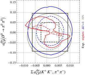
We find that for such an -breaking scenario, the different NP models start to imply different patterns. This is illustrated in Fig. 4, where we observe a correlation between the signs of and in the triplet model.
The capability to differentiate between the different models will improve significantly with future data. With present data, however, it is already possible to exclude many scenarios for breaking, as the exclusion of the pure triplet enhancement demonstrated in Section III.3.
The future data scenario is designed having in mind the model being realized. The goal is to determine whether this model can be distinguished from the others by data, despite its many CP violating contributions. We find that all NP models remain capable of fitting the future data set well, despite its somewhat specific construction, with for the HN model and for the others. In Fig. 5, we show exemplarily correlations for the various models as in Fig. 4.
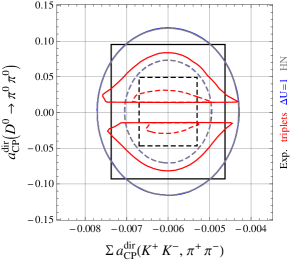
While for the shown observables the model cannot be distinguished from the HN model, in MFV/SM and the triplet model a clear prediction of a sizable CP asymmetry in emerges. This serves as a confirmation that in principle the various scenarios are distinguishable within our framework. However, as is obvious comparing Figs. 4 and 5, further dynamical input on breaking would facilitate this task enormously.
V Conclusions
We performed a comprehensive -flavor analysis using the complete set of data on two-body decays of -mesons to pseudoscalar octet mesons. The results are based on plain ; in particular, we did not make any assumptions about decay topologies nor assumed factorizable -breaking. We find
-
i
The -expansion can describe the CF, SCS and DCS data set with breaking of .
-
ii
-breaking matrix elements involving higher representations cannot be neglected.
-
iii
Current data imply significantly enhanced penguin matrix elements with respect to the non-triplet ones, see Figure 2. If the measured largish CP asymmetries in , and decays are excluded from the fit the penguin enhancement is shifted to smaller but still significantly enhanced values at , see Figure 3, favoring interpretations within NP models. Improved data could clarify how large the penguin enhancement actually needs to be.
The model-independence of the -expansion leads to a large number of -breaking matrix elements, and the outcome of the fits currently does not allow an unambiguous interpretation regarding the underlying electroweak physics. In more minimal scenarios, where -breaking is limited to a smaller number of matrix elements, clearer patterns exist, see Figure 4. In addition, it is possible already with present data to differentiate between various -breaking structures.
Keeping all matrix elements, the following measurements of direct CP violation are found to be informative for discriminating scenarios:
- iv
-
v
An observation of a finite would signal new physics. The current hint with large central value already favors the Hamiltonian, an example of which is provided by Hochberg:2011ru . The operator enhancement from the current fit is, given the uncertainties, in the ballpark of what is required to explain the current anomalies in the top sector.
-
vi
We predict that is enhanced with respect to , see Eq. (32).
Future fits with improved data on charm CP violation Bediaga:2012py ; Aushev:2010bq ; O'Leary:2010af ; Asner:2008nq will shed light on the origin of CP and flavor violation in charm.
Note added: While this work has been completed, a related study appeared Grossman:2012ry .
Acknowledgements.
This project is supported in part by the German-Israeli foundation for scientific research and development (GIF) and the Bundesministerium für Bildung und Forschung (BMBF). GH gratefully acknowledges the kind hospitality of the theory group at DESY Hamburg, where parts of this work have been done. StS thanks Christian Hambrock for useful exchanges.Appendix A Subtracting indirect CP asymmetries
Decays with a in the final state receive an additional contribution to the CP asymmetry from kaon mixing. To isolate the direct CP asymmetry, we subtract the mixing contribution . For a decay with a () in the flavor final state, the mixing contribution to its CP asymmetry is given by () Cenci:2012uy . Therefore,
| (34) | ||||
| (35) |
As pointed out in Grossman:2011zk , the actual influence of kaon mixing depends on the experiment, due to its dependence on the kaon decay time. In the most recent analyses Cenci:2012uy ; CKM12:Ko this effect is accounted for.
To obtain , we took into account the effect of mixing in the same way as kaon mixing and subtracted .
Indirect CP violation in both kaon and charm mixing is discarded in , as for this mode the experimental uncertainties are much larger than these effects.
To calculate , we average the data from CDF and the B-factories, taking into account the correlations between and . In order to obtain , we subtract the contribution from indirect CP violation. We find the correlation coefficient between and to be only , which we can safely neglect in our analysis. The reason for the small correlation lies in the small impact of the -factory results and on the average of .
Appendix B Amplitudes including breaking
In this appendix, the coefficient tables for the -breaking parts of the amplitudes are given. In Table 4 we list the coefficients for the full set of matrix elements, before reducing the basis to include only physical ones. The coefficients for the latter are given in Table 5.
| Decay | |||||||||||||||
| SCS | |||||||||||||||
| CF | |||||||||||||||
| DCS | |||||||||||||||
| Decay | ||||||||
|---|---|---|---|---|---|---|---|---|
| SCS | ||||||||
| CF | ||||||||
| DCS | ||||||||
Appendix C Future data scenario
To obtain estimates for the experimental uncertainties in the future data scenario, we make the following assumptions: we assume that the systematic uncertainty on given in Aaij:2011in improves by a factor and dominates the statistical uncertainty; furthermore, we assume several CP asymmetries to be measured with the same precision as , see Table 3. The prospect for the uncertainty of the strong phase is taken from CKM12:Asner .
As in the model there is NP in the coupling, we assume that and are enhanced, whereas and . Furthermore, in the triplet model the observables , and are all determined uniquely by , whereas does not contribute here. It is therefore difficult in the triplet model to account for these three CP asymmetries not being of the same order of magnitude. Consequently, we assume to stay large. All assumed central values are within the interval of the current measurements listed in Table 2.
Note that the expectation that the operator in the model contributes mainly to matrix elements with kaons is not a statement from . It would amount to additional dynamical input, which we avoid in this work. Such assumptions could be implemented by assuming relations between matrix elements.
References
- (1) R. Aaij et al. [LHCb Collaboration], Phys. Rev. Lett. 108, 111602 (2012) [arXiv:1112.0938 [hep-ex]].
- (2) T. Aaltonen et al. [CDF Collaboration], Phys. Rev. Lett. 109, 111801 (2012) [arXiv:1207.2158 [hep-ex]].
- (3) B. R. Ko for the Belle Collaboration, Talk at the 36th International Conference for High Energy Physics (ICHEP), 4-11 July 2012 Melbourne, Australia.
- (4) Y. Amhis et al. [Heavy Flavor Averaging Group Collaboration], arXiv:1207.1158 [hep-ex] and online update http://www.slac.stanford.edu/xorg/hfag/charm from April 2012.
- (5) R. L. Kingsley, S. B. Treiman, F. Wilczek and A. Zee, Phys. Rev. D 11 (1975) 1919.
- (6) M. B. Einhorn and C. Quigg, Phys. Rev. D 12, 2015 (1975).
- (7) G. Altarelli, N. Cabibbo and L. Maiani, Nucl. Phys. B 88, 285 (1975).
- (8) M. B. Voloshin, V. I. Zakharov and L. B. Okun, JETP Lett. 21, 183 (1975) [Pisma Zh. Eksp. Teor. Fiz. 21, 403 (1975)].
- (9) C. Quigg, Z. Phys. C 4, 55 (1980).
- (10) M. J. Savage, Phys. Lett. B 257 (1991) 414.
- (11) L. -L. Chau and H. -Y. Cheng, Phys. Lett. B 280, 281 (1992).
- (12) D. Pirtskhalava and P. Uttayarat, Phys. Lett. B 712, 81 (2012) [arXiv:1112.5451 [hep-ph]].
- (13) T. Feldmann, S. Nandi and A. Soni, JHEP 1206, 007 (2012) [arXiv:1202.3795 [hep-ph]].
- (14) J. Brod, Y. Grossman, A. L. Kagan and J. Zupan, JHEP 1210, 161 (2012) [arXiv:1203.6659 [hep-ph]].
- (15) J. Brod, A. L. Kagan and J. Zupan, Phys. Rev. D 86, 014023 (2012) [arXiv:1111.5000 [hep-ph]].
- (16) H. -Y. Cheng and C. -W. Chiang, Phys. Rev. D 85, 034036 (2012) [arXiv:1201.0785 [hep-ph]].
- (17) B. Bhattacharya, M. Gronau and J. L. Rosner, Phys. Rev. D 85, 054014 (2012) [arXiv:1201.2351 [hep-ph]].
- (18) H. -n. Li, C. -D. Lu and F. -S. Yu, Phys. Rev. D 86, 036012 (2012) [arXiv:1203.3120 [hep-ph]].
- (19) E. Franco, S. Mishima and L. Silvestrini, JHEP 1205, 140 (2012) [arXiv:1203.3131 [hep-ph]].
- (20) J. J. de Swart, Rev. Mod. Phys. 35, 916 (1963) [Erratum-ibid. 37, 326 (1965)].
- (21) T. A. Kaeding, nucl-th/9502037.
- (22) T. A. Kaeding and H. T. Williams, Comput. Phys. Commun. 98, 398 (1996) [nucl-th/9511025].
- (23) G. Hiller, M. Jung and S. Schacht, in preparation.
- (24) I. Hinchliffe and T. A. Kaeding, Phys. Rev. D 54, 914 (1996) [hep-ph/9502275].
- (25) F. Buccella, M. Lusignoli, G. Mangano, G. Miele, A. Pugliese and P. Santorelli, Phys. Lett. B 302, 319 (1993) [hep-ph/9212253].
- (26) Y. Grossman, A. L. Kagan and J. Zupan, Phys. Rev. D 85, 114036 (2012) [arXiv:1204.3557 [hep-ph]].
- (27) W. Kwong and S. P. Rosen, Phys. Lett. B 298, 413 (1993).
- (28) A.R. Conn, N.I.M. Gould and P. Toint, SIAM J. Numer. Anal. 28,2 (1991) 545–572.
- (29) E. G. Birgin and J. M. Martínez, Optimization Methods and Software 23,2 (2008) 177–195.
- (30) S. G. Johnson, http://ab-initio.mit.edu/nlopt.
- (31) T. Rowan, PhD thesis, Department of Computer Sciences, University of Texas at Austin, 1990.
- (32) L. F. Abbott, P. Sikivie and M. B. Wise, Phys. Rev. D 21, 768 (1980).
- (33) M. Golden and B. Grinstein, Phys. Lett. B 222, 501 (1989).
- (34) J. Beringer et al. [Particle Data Group Collaboration], Phys. Rev. D 86, 010001 (2012).
- (35) A. F. Falk, Y. Grossman, Z. Ligeti and A. A. Petrov, Phys. Rev. D 65, 054034 (2002) [hep-ph/0110317].
- (36) B. Bhattacharya and J. L. Rosner, Phys. Rev. D 81, 014026 (2010) [arXiv:0911.2812 [hep-ph]].
- (37) B. Aubert et al. [BaBar Collaboration], Phys. Rev. Lett. 100, 061803 (2008) [arXiv:0709.2715 [hep-ex]].
- (38) M. Staric et al. [Belle Collaboration], Phys. Lett. B 670, 190 (2008) [arXiv:0807.0148 [hep-ex]].
- (39) T. Aaltonen et al. [CDF Collaboration], Phys. Rev. D 85, 012009 (2012) [arXiv:1111.5023 [hep-ex]].
- (40) G. Bonvicini et al. [CLEO Collaboration], Phys. Rev. D 63, 071101 (2001) [hep-ex/0012054].
- (41) H. Mendez et al. [CLEO Collaboration], Phys. Rev. D 81, 052013 (2010) [arXiv:0906.3198 [hep-ex]].
- (42) R. Cenci [on behalf of the BaBar Collaboration], arXiv:1209.0138 [hep-ex].
- (43) J. M. Link et al. [FOCUS Collaboration], Phys. Rev. Lett. 88, 041602 (2002) [Erratum-ibid. 88, 159903 (2002)] [hep-ex/0109022].
- (44) B. R. Ko for the Belle Collaboration, Talk at the 7th International Workshop on the CKM Unitarity Triangle, 28 September - 2 October 2012, Cincinnati, Ohio, USA.
- (45) B. R. Ko et al. [Belle Collaboration], Phys. Rev. Lett. 104, 181602 (2010) [arXiv:1001.3202 [hep-ex]].
- (46) M.-Z. Wang for the Belle Collaboration, Talk at the 36th International Conference for High Energy Physics (ICHEP), 4-11 July 2012 Melbourne, Australia.
- (47) G. Isidori, J. F. Kamenik, Z. Ligeti and G. Perez, Phys. Lett. B 711, 46 (2012) [arXiv:1111.4987 [hep-ph]].
- (48) Y. Grossman, A. L. Kagan, Y. Nir, Phys. Rev. D75, 036008 (2007) [hep-ph/0609178].
- (49) G. F. Giudice, G. Isidori and P. Paradisi, JHEP 1204, 060 (2012) [arXiv:1201.6204 [hep-ph]].
- (50) G. Hiller, Y. Hochberg and Y. Nir, Phys. Rev. D 85, 116008 (2012) [arXiv:1204.1046 [hep-ph]].
- (51) L. Da Rold, C. Delaunay, C. Grojean and G. Perez, arXiv:1208.1499 [hep-ph].
- (52) Y. Hochberg and Y. Nir, Phys. Rev. Lett. 108, 261601 (2012) [arXiv:1112.5268 [hep-ph]].
- (53) W. Altmannshofer, R. Primulando, C. -T. Yu and F. Yu, JHEP 1204, 049 (2012) [arXiv:1202.2866 [hep-ph]].
- (54) A. J. Buras, M. Misiak and J. Urban, Nucl. Phys. B 586, 397 (2000) [hep-ph/0005183].
- (55) G. Hiller and F. Kruger, Phys. Rev. D 69, 074020 (2004) [hep-ph/0310219].
- (56) G. Isidori and J. F. Kamenik, Phys. Rev. Lett. 109, 171801 (2012) [arXiv:1205.3164 [hep-ph]].
- (57) T. Aaltonen et al. [CDF Collaboration], arXiv:1211.1003 [hep-ex].
- (58) G. Aad et al. [ATLAS Collaboration], Eur. Phys. J. C 72, 2039 (2012) [arXiv:1203.4211 [hep-ex]].
- (59) [CMS Collaboration], CMS-PAS-TOP-11-014.
- (60) J. Drobnak, A. L. Kagan, J. F. Kamenik, G. Perez and J. Zupan, arXiv:1209.4872 [hep-ph].
- (61) I. Bediaga et al. [LHCb Collaboration], arXiv:1208.3355 [hep-ex].
- (62) T. Aushev, W. Bartel, A. Bondar, J. Brodzicka, T. E. Browder, P. Chang, Y. Chao and K. F. Chen et al., arXiv:1002.5012 [hep-ex].
- (63) B. O’Leary et al. [SuperB Collaboration], arXiv:1008.1541 [hep-ex].
- (64) D. M. Asner, T. Barnes, J. M. Bian, I. I. Bigi, N. Brambilla, I. R. Boyko, V. Bytev and K. T. Chao et al., Int. J. Mod. Phys. A 24, S1 (2009) [arXiv:0809.1869 [hep-ex]].
- (65) Y. Grossman and D.J. Robinson, arXiv:1211.3361 [hep-ph].
- (66) Y. Grossman and Y. Nir, JHEP 1204, 002 (2012) [arXiv:1110.3790 [hep-ph]].
- (67) D. Asner for the Belle II Collaboration, Talk at the 7th International Workshop on the CKM Unitarity Triangle, 28 September - 2 October 2012, Cincinnati, Ohio, USA.