Constraints on a MOND effect for isolated aspherical systems in deep Newtonian regime from orbital motions

Abstract

The dynamics of non-spherical systems described by MOND theories arising from generalizations of the Poisson equation is affected by an extra MONDian quadrupolar potential $\phi_{\rm Q}$ even if they are isolated (no EFE effect) and if they are in deep Newtonian regime. In general MOND theories quickly approaching Newtonian dynamics for accelerations beyond $A_{0}$, $\phi_{\rm Q}$ is proportional to a coefficient $\alpha\sim 1$, while in MOND models becoming Newtonian beyond $\kappa A_{0},\ \kappa\gg 1,$ it is enhanced by $\kappa^{2}$. We analytically work out some orbital effects due to $\phi_{\rm Q}$ in the framework of QUMOND, and compare them with the latest observational determinations of Solar System’s planetary dynamics, exoplanets, double lined spectroscopic binary stars and binary radio pulsars. The current admissible range for the anomalous perihelion precession of Saturn $-0.5$ milliarcseconds per century $\leq\Delta\dot{\varpi}\leq 0.8$ milliarcseconds per century yields $|\kappa|\leq{\color[rgb]{0,0,0}3}.5\times 10^{{\color[rgb]{0,0,0}3}}$, while the radial velocity of $\alpha$ Cen AB allows to infer $|\kappa|\leq 6.2\times 10^{4}\ ({\rm A})$ and $|\kappa|\leq 4.2\times 10^{4}\ ({\rm B})$.

PACS: 04.80.-y; 04.80.Cc; 95.1O.Ce; 95.10.Km; 97.80.-d

1 Introduction

The MOdified Newtonian Dynamics (MOND) (see [1] for a recent review) is a theoretical framework proposed by Milgrom [2, 3, 4] to modify the laws of the gravitational interaction in a suitably defined low acceleration regime to explain the observed anomalous kinematics of certain astrophysical systems such as various kinds of galaxies [5, 6, 7]. Indeed, their behaviour does not agree with the predictions made with the usual Newtonian inverse-square law applied to the electromagnetically detected baryonic matter whose quantity appears to be insufficient. In the case of the mass discrepancy occurring in clusters of galaxies [8], MOND actually faces difficulties in explaining it [9, 10, 11]. In almost all its relativistic formulations, MOND implies a single acceleration scale [13] $A_{0}=(1.2\pm 0.27)\times 10^{-10}$ m s^-2 below which the laws of gravitation would suffer notable modifications mimicking the effect of the additional non-baryonic Dark Matter which is usually invoked to explain the observed discrepancy within the standard theoretical framework.

In this paper, we propose to constrain a recently predicted strong-field effect of MOND [14] by using various observables pertaining different astronomical scenarios. In the following we will briefly outline the main features of such a novel prediction of MOND which occurs even if the system under consideration is isolated and if its characteristic accelerations are quite larger than $A_{0}$.

Let us consider an isolated, strongly gravitating system $\mathcal{S}$ of total mass $M_{\rm tot}$ and extension

$$R\ll d_{\rm M}\doteq\sqrt{{GM_{\rm tot}\over A_{0}}},$$ (1)

where $G$ is the Newtonian constant of gravitation. Let us also assume that the mass distribution of $\mathcal{S}$, characterized by a generally anisotropic matter density $\varrho(\boldsymbol{r})$, varies over timescales much larger than $t_{\rm M}\doteq d_{\rm M}/c,$ where $c$ is the speed of light in vacuum. According to formulations of MOND based on extensions of the Poisson equation such as the nonlinear Poisson model by Bekenstein and Milgrom [15] and QUMOND [17], it turns out [14] that, if on the one hand, the MOND field equations of $\mathcal{S}$ coincide with the usual linear Poisson equation for $r\leq R$ depending on how the MOND interpolating function $\mu$ is close to unity, on the other hand, they differ from it for $r\geq d_{\rm M}$. This is a crucial feature since it implies that the solution $\phi$ of the Poisson equation for $r\leq R$ is, in general, different from the usual Newtonian one $\phi_{\rm N}$, thus affecting the internal dynamics of $\mathcal{S}$ even if it is in the strong gravity regime. It is as if a hollow “phantom” matter distribution, characterized by a phantom matter density $\varrho_{\rm ph}(\boldsymbol{r})$, was present at $r\geq d_{\rm M}$ in such a way that, in the quasi-static limit previously defined, $\varrho(\boldsymbol{r})$ instantaneously controls $\varrho_{\rm ph}(\boldsymbol{r})$ by fixing its symmetry properties. If $\varrho=\varrho(r)$, i.e. if $\mathcal{S}$ is spherically symmetric, then the phantom matter density is spherically symmetric as well. In this case, the internal dynamics of $\mathcal{S}$ would not be affected by the peculiar boundary conditions on the MOND field equations at $r\geq d_{\rm M}$ or, equivalently, by the phantom matter. Indeed, it would be arranged in a hollow spherical shell; the dynamics of $\mathcal{S}$ would be Newtonian to the extent that the MOND interpolating function $\mu$ matches the unity. On the contrary, if $\varrho=\varrho(\boldsymbol{r})$, i.e. if $\mathcal{S}$ is not spherically symmetric, the same occurs to the phantom matter as well. Thus, it does have an influence on the internal dynamics of $\mathcal{S}$ which, to the lowest order, can be approximated by an additional quadrupolar potential $\phi_{Q}=\phi-\phi_{\rm N}$.

By assuming $\mu=1$ to the desired accuracy everywhere within $\mathcal{S}$ and by using QUMOND [17], Milgrom [14] obtained

$$\phi_{Q}({\boldsymbol{r}}_{F})=-{\alpha G\over{\color[rgb]{0,0,0}d}^{5}_{\rm M}}x_{F}^{i}x_{F}^{j}Q_{ij}$$ (2)

with

$$Q_{ij}\doteq{1\over 2}\int_{\mathcal{S}}\varrho\left({\boldsymbol{r}}^{{}^{\prime}}\right)\left(r^{{}^{\prime}2}\delta_{ij}-3x_{i}^{{}^{\prime}}x_{j}^{{}^{\prime}}\right)d{\boldsymbol{r}}^{{}^{\prime}};$$ (3)

$x_{F}^{i},i=1,2,3$ in eq. (2) are the components of the position vector ${\boldsymbol{r}}_{F}$ of a generic point F with respect to the barycenter of $\mathcal{S}$, while $x^{{}^{\prime}}_{j},j=1,2,3$ in eq. (3) determine the barycentric position of the system’s mass elements. The coefficient $\alpha$ depends on the specific form of the interpolating function chosen. Milgrom [14], by considering also the case in which the strong field regime is obtained in terms of a second, dimensionless constant $\kappa\gg 1$ when the Newtonian acceleration is as large as $\sim\kappa A_{0}$, picked up an interpolating function yielding

$$\alpha_{\kappa}=\kappa^{2}\alpha_{\kappa=1},\ \alpha_{\kappa=1}\sim 1.$$ (4)

In general, there should be many other interpolating functions that could be used with $\kappa\gg 1$; in this paper, we will focus on eq. (4). Finally, we remark that Milgrom [14] felt that theories with $\kappa\gg 1$ cannot be considered as generic MOND results.

As stressed by Milgrom [14], the quadrupolar MOND effect of eq. (2) has not to be confused with some other MONDian features occurring in the strong acceleration regime which were previously examined in literature. In particular, it is not the quadrupolar effect [18, 19] due to the External Field Effect (EFE) [2, 15, 20] arising when the system under consideration is immersed in an external background field; indeed, here the system is considered isolated. Even so, residual MONDian effects in the strong acceleration regime exist, in general, because of the remaining departure of $\mu(q)$ from 1 when $q\gg 1$; their consequences on orbital motions of Solar System objects were treated in, e.g., [2, 21, 22, 18]. Nonetheless, they are different from the presently studied effect, for which it was posed $\mu=1$ to the desired accuracy. Finally, Milgrom [14] showed that the impact of the zero-gravity points [23, 24, 25] existing in high acceleration regions on the dynamics of the mass sources themselves is negligible with respect to the effect considered here.

The plan of the paper is as follows. In Section 2 we analytically work out some orbital effects caused by eq. (2) to an isolated two-body system in the case of eq. (4). In Section 3 our results are compared to latest observations on Solar System planetary motions, extrasolar planets, and spectroscopic binary stars. Section 4 is devoted to summarizing our findings.

2 Calculation of some orbital effects

Let us consider a typical non-spherical system such as a localized binary made of two point masses $M$ and $m$ with $M_{\rm b}\doteq M_{\rm tot}=M+m$. In a barycentric frame, its mass density $\varrho\left({{\boldsymbol{r}}_{F}}\right)$ at a generic point F can be posed

$${\color[rgb]{0,0,0}\varrho}\left({{\boldsymbol{r}}_{F}}\right)=M\delta^{3}\left({{\boldsymbol{r}}_{F}}-{\boldsymbol{r}}_{M}\right)+m\delta^{3}\left({{\boldsymbol{r}}_{F}}-{\boldsymbol{r}}_{m}\right),$$ (5)

where ${\boldsymbol{r}}_{m}$ and ${\boldsymbol{r}}_{M}$ are the barycentric position vectors of $m$ and $M$, respectively.

After having calculated $\phi_{Q}({\boldsymbol{r}}_{F})$ for eq. (5), its gradient with respect to ${\boldsymbol{r}}_{F}$ yields the extra-acceleration ${\boldsymbol{A}}_{F}$ of an unit mass at a generic point $F$. The extra-accelerations ${\boldsymbol{A}}_{m}$ and ${\boldsymbol{A}}_{M}$ experienced by $m$ and $M$ can be obtained by calculating ${\boldsymbol{A}}_{F}$ for ${\boldsymbol{r}}_{m}=MM_{\rm b}^{-1}\boldsymbol{r}$ and for ${\boldsymbol{r}}_{M}=-mM_{\rm b}^{-1}\boldsymbol{r}$, respectively, where $\boldsymbol{r}\doteq{\boldsymbol{r}}_{m}-{\boldsymbol{r}}_{M}$ is the relative position vector directed from $M$ to $m$. It turns out that the accelerations felt by $m$ and $M$ are

$${\boldsymbol{A}}_{m} =-{2\alpha A_{0}mM^{2}\over M^{3}_{\rm b}d^{3}_{\rm M}}r^{2}\boldsymbol{r},$$ (6)

$${\boldsymbol{A}}_{M} ={2\alpha A_{0}Mm^{2}\over M^{3}_{\rm b}d^{3}_{\rm M}}r^{2}\boldsymbol{r}.$$ (7)

The relative extra-acceleration is, thus, [14]

$$\boldsymbol{A}=-{2\alpha A_{0}\over d^{3}_{\rm M}}\left({\mu_{\rm b}\over M_{\rm b}}\right)r^{2}\boldsymbol{r},$$ (8)

where $\mu_{\rm b}\doteq mMM_{\rm b}^{-1}$ is the binary’s reduced mass. For the following developments, it is useful to remark that, formally, eq. (8) can be derived from the effective potential

$$U_{\rm M}={\alpha A_{0}\over 2d^{3}_{\rm M}}\left({\mu_{\rm b}\over M_{\rm b}}\right)r^{4}.$$ (9)

2.1 The pericenter rate for a two-body MOND quadrupole

The longitude of pericenter $\varpi\doteq\mathit{\Omega}+\omega$ is a “broken” angle since the longitude of the ascending node $\mathit{\Omega}$ lies in the reference $\left\{x,y\right\}$ plane from the reference $x$ direction to the line of the nodes, while the argument of pericenter $\omega$ reckons the position of the point of closest approach in the orbital plane with respect to the line of the nodes. The angle $\varpi$ is usually adopted in Solar System studies to put constraints on putative modifications of standard Newtonian/Einsteinian dynamics [26]. Its Lagrange perturbation equation is [27]

$$\left\langle\frac{{{d}}{\varpi}}{{{d}}{t}}\right\rangle=-{1\over n_{\rm b}a^{2}}\left[\left({\sqrt{1-e^{2}}\over e}\right){\partial{\left\langle U_{\rm pert}\right\rangle}\over\partial{e}}+{\tan\left({I\over 2}\right)\over\sqrt{1-e^{2}}}{\partial{\left\langle U_{\rm pert}\right\rangle}\over\partial{I}}\right],$$ (10)

where $U_{\rm pert}$ is a small correction to the Newtonian potential; $a$ is the relative semimajor axis, $e$ is the orbital eccentricity, and $I$ is the inclination of the orbital plane to the reference $\left\{x,y\right\}$ plane. The brackets $\left\langle\ldots\right\rangle$ in eq. (10) denote the average over one full orbital period $P_{\rm b}=2\pi n_{\rm b}^{-1}=2\pi\sqrt{a^{3}G^{-1}M_{\rm b}^{-1}}$. By adopting eq. (9) as perturbing potential $U_{\rm pert}$ in eq. (10), one gets

$$\left\langle\frac{{{d}}{\varpi}}{{{d}}{t}}\right\rangle=-{5\alpha A_{0}P_{\rm b}\over 2\pi d_{\rm M}}\left({\mu_{\rm b}\over M_{\rm b}}\right)\left({a\over d_{\rm M}}\right)^{2}\sqrt{1-e^{2}}\left(1+{3\over 4}e^{2}\right).$$ (11)

It should be remarked that eq. (9) and, thus, eq. (11) are valid just for a two-body MOND quadrupole $Q_{ij}$.

As a cross-check of the validity of our result, we repeated the calculation of the long-term precession of $\varpi$ by using eq. (8) as perturbing acceleration and the Gauss equations for the variations of the elements: we re-obtained eq. (11).

2.2 The timing in binary radiopulsars

The basic observable in binary pulsar systems is the periodic change $\delta\tau_{\rm p}$ in the time of arrivals (TOAs) $\tau_{\rm p}$ of the pulsar p due to the fact that it is gravitationally bounded to a generally unseen companion c, thus describing an orbital motion around the common barycenter. In a binary hosting an emitting radiopulsar, the Keplerian expression of $\delta\tau_{\rm p}$ is obtained by taking the ratio of the component $\rho_{\rm p}$ of the barycentric pulsar’s orbit along the line of sight to the speed of light $c$. Thus, one has

$$\delta\tau_{\rm p}={\rho_{\rm p}\over c}.$$ (12)

Since the line of sight is customarily assumed as reference $z$ axis, in eq. (12) it is

$$\rho_{\rm p}\equiv z_{\rm p},\ z_{\rm p}=r_{\rm p}\sin I\sin(\omega+f),$$ (13)

as it can be inferred from the standard expressions for the orientation of the Keplerian ellipse in space. In eq. (13), $r_{\rm p}$ is the distance of the pulsar from the system’s center of mass, $I$ is the inclination of the orbit to the plane of the sky, assumed as reference $\{x,y\}$ plane, and $f$ is the true anomaly reckoning the instantaneous position of the pulsar with respect to the periastron position. By using

$$r_{\rm p} =a_{\rm p}(1-e\cos E),$$ (14)

$$\cos f ={\cos E-e\over 1-e\cos E},$$ (15)

$$\sin f ={\sqrt{1-e^{2}}\sin E\over 1-e\cos E},$$ (16)

where $a_{\rm p}$ is the semimajor axis of the the pulsar’s barycentric orbit and $E$ is the eccentric anomaly, from eq. (12)-eq. (13) one straightforwardly gets [28, 29]

$$\delta\tau_{\rm p}={\rm x}_{\rm p}\left[\left(\cos E-e\right)\sin\omega+\sqrt{1-e^{2}}\sin E\cos\omega\right].$$ (17)

In eq. (17), ${\rm x}_{\rm p}\doteq a_{\rm p}\sin I/c$ is the projected semimajor axis of the pulsar’s barycentric orbit and has dimensions of time; by posing $m_{\rm p}\doteq M,m_{\rm c}\doteq m$, it is $a_{\rm p}{\color[rgb]{0,0,0}\doteq}a_{M}=mM^{-1}_{\rm b}a,$ where $a$ is the semimajor axis of the pulsar-companion relative orbit.

In general, the shift per orbit $\Delta Y$ of an observable $Y$ with respect to its classical expression due to the action of a perturbing acceleration such as either eq. (6) or eq. (7) can be computed as

$$\Delta Y=\int_{0}^{P_{\rm b}}\left(\frac{{{d}}{Y}}{{{d}}{t}}\right)dt=\int_{0}^{2\pi}\left[{\partial{Y}\over\partial{E}}\frac{{{d}}{E}}{{{d}}{\mathcal{M}}}\frac{{{d}}{\mathcal{M}}}{{{d}}{t}}+\sum_{\psi}{\partial{Y}\over\partial{\psi}}\frac{{{d}}{\psi}}{{{d}}{t}}\right]\left(\frac{{{d}}{t}}{{{d}}{E}}\right)dE,$$ (18)

where ${\mathcal{M}}$ is the mean anomaly and $\psi$ collectively denotes the other Keplerian orbital elements. The rates $\dot{\mathcal{M}},\dot{\psi}$ entering eq. (18) are due to the perturbation and are instantaneous. As such, they are obtained by computing the right-hand-sides of either the Lagrange equations or the Gauss equations onto the unperturbed Keplerian ellipse without averaging them over $P_{\rm b}$. The derivatives $\partial Y/\partial E,\partial Y/\partial\psi$ in eq. (18) are computed by using the unperturbed expression for $Y$.

By using eq. (18) and

$${dt\over dE}={1-e\cos E\over n_{\rm b}},$$ (19)

the MOND time shift perturbation can be computed as

$$\Delta\delta\tau_{\rm p}=-{7\alpha A_{0}P^{2}_{\rm b}\over 8\pi c}\left({m\mu_{\rm b}\over M_{\rm b}^{2}}\right)\left({a\over d_{\rm M}}\right)^{3}e\sqrt{1-e^{2}}\left(1+{e^{2}\over 2}\right)\cos\omega\sin I.$$ (20)

It is important to notice that eq. (20) is proportional to $P^{2}_{\rm b}$ and to $e$. At a first sight, it may be weird to see in eq. (20) a dependence on the speed of light $c$ in a non-relativistic theory such as QUMOND; actually, it is not so because of the definition of $\tau_{\rm p}$ in eq. (12).

2.3 The radial velocity

The radial velocity $V_{\rho_{\rm lc}}$ [30] is a standard observable in spectroscopic studies of binaries [31]. Up to the radial velocity of the binary’s center of mass $V_{0}$, the Keplerian expression of the radial velocity of the component of the binary whose light curve (lc) is available can be obtained by taking the time derivative of the projection $\rho_{\rm lc}$ of the barycentric orbit of the visible component onto the line of sight. Thus, from eq. (13), it can be posed

$$V_{\rho_{\rm lc}}=\frac{{{d}}{\rho_{\rm lc}}}{{{d}}{t}}\equiv\frac{{{d}}{z_{\rm lc}}}{{{d}}{t}}={\partial{z_{\rm lc}}\over\partial{f}}{\partial{f}\over\partial{{\mathcal{M}}}}n_{\rm b}.$$ (21)

By using the standard Keplerian expressions

$${\partial{f}\over\partial{{\mathcal{M}}}} =\left({a_{\rm lc}\over r_{\rm lc}}\right)^{2}\sqrt{1-e^{2}},$$ (22)

$$r_{\rm lc} ={a_{\rm lc}(1-e^{2})\over 1+e\cos f},$$ (23)

where $r_{\rm lc}$ and $a_{\rm lc}$ refer to the barycentric orbit of the visible partner, eq. (21) straightforwardly yields

$$V_{\rho_{\rm lc}}=K\left[e\cos\omega+\cos\left(\omega+f\right)\right]={n_{\rm b}a_{\rm lc}\sin I\over\sqrt{1-e^{2}}}\left[e\cos\omega+\cos\left(\omega+f\right)\right].$$ (24)

In eq. (24), $K$ is the semi-amplitude of the radial velocity. In the case of extrasolar planetary systems, the light curve is usually available only for the hosting star; thus, $a_{\rm lc}{\color[rgb]{0,0,0}\doteq}a_{M}=mM^{-1}_{\rm b}a$. In the case of spectroscopic binary stars, it may happen that the light curves of both the components (double lined spectroscopic binary stars) are available.

As for $\Delta\delta\tau_{\rm p}$, also the perturbation $\Delta V_{\rho_{\rm lc}}$ of the radial velocity due to a disturbing extra-acceleration can be calculated from eq. (18). In this case, it is computationally more convenient to replace $E$ with $f$ throughout eq. (18); as a consequence,

$$\frac{{{d}}{t}}{{{d}}{f}}={\left(1-e^{2}\right)^{3/2}\over n_{\rm b}\left(1+e\cos f\right)^{2}}$$ (25)

must be used. The MOND perturbation of $V_{\rho_{\rm lc}}$ turns out to be

$$\Delta V_{\rho_{\rm lc}}={17\over 2}\alpha A_{0}P_{\rm b}\left({m\mu_{\rm b}\over M_{\rm b}^{2}}\right)\left({a\over d_{\rm M}}\right)^{3}e\left(1+{8\over 17}e^{2}\right)\sin I\sin\omega.$$ (26)

It is important to note the proportionality of eq. (26) to $P_{\rm b}$ and to $e$.

3 Confrontation with the observations

3.1 Planets of the Solar System

As far as the Solar System is concerned, $t_{\rm M}=39$ d; thus the quasi-staticity condition is fully satisfied by the gaseous giant planets for which it is $P_{\rm b}\gtrsim 4300$ d.

Among them, Saturn, whose orbital period is as large as $P_{\rm b}=10759$ d, is the most suitable to effectively constrain $\alpha$ since its orbit is nowadays known with $\approx 20$ m accuracy [26] in view of the multi-year record of accurate radio-technical data from the Cassini spacecraft. Looking at its perihelion, any deviation of its secular precession from the rate predicted by the standard Newtonian/Einsteinian dynamics can nowadays be constrained down to sub-milliarcseconds per century (mas cty^-1) level, as shown by Table 1.

Table 1: Supplementary precessions $\Delta\dot{\mathit{\Omega}},\Delta\dot{\varpi}$ of the longitudes of the node and of the perihelion for some planets of the Solar System estimated by Fienga et al. [26] with the INPOP10a ephemerides. Data from Messenger and Cassini were used. Fienga et al. [26] fully modeled all standard Newtonian/Einsteinian dynamics, apart from the Solar Lense-Thirring effect, which, however, is relevant only for Mercury; MOND was not modelled. The reference $\{x,y\}$ plane is the mean Earth’s equator at J$2000.0$. The units are milliarcseconds per century (mas cty^-1).

	$\Delta\dot{\mathit{\Omega}}$ (mas cty-1)	$\Delta\dot{\varpi}$ (mas cty-1)
Mercury	$1.4\pm 1.8$	$0.4\pm 0.6$
Venus	$0.2\pm 1.5$	$0.2\pm 1.5$
Earth	$0.0\pm 0.9$	$-0.2\pm 0.9$
Mars	$-0.05\pm 0.13$	$-0.04\pm 0.15$
Saturn	$-0.1\pm 0.4$	$0.15\pm 0.65$

If the case $\alpha_{\kappa}=\kappa^{2}\alpha_{\kappa=1}$, with $\alpha_{\kappa=1}\sim 1$ is considered, the two-body expression of eq. (11) and Table 1 yield

$$|\kappa|\leq 2.5\times 10^{5};$$ (27)

larger values for $|\kappa|$ would yield an anomalous secular perihelion precession exceeding the allowed bounds in Table 1.

Actually, our analysis is incomplete since it is limited to a two-body scenario. As remarked by Milgrom himself [14], also the contribution of the other planets, especially the more massive ones, should be taken into account in the mass density $\varrho$ of $\mathcal{S}$ in eq. (3). The resulting constraints on $\kappa$ may, thus, be altered with respect to eq. (27). We will face this issue in a numerical way by integrating the barycentric equations of motion of the Sun, Jupiter, Saturn, Uranus and Neptune modified with the inclusion of the accelerations due to eq. (2). Moreover, eq. (3) will be calculated by taking into account the contributions of Jupiter, Uranus and Neptune as well. The result is depicted in Figure 1.

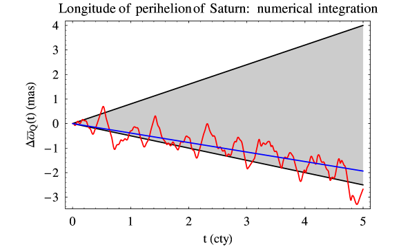
Figure 1: Gray-shaded area: allowed region for any anomalous perihelion precession $\Delta\dot{\varpi}$ of Saturn according to the constraints in Table 1. The black straight lines delimiting it represent the secular perihelion shifts of Saturn corresponding to $\Delta\dot{\varpi}_{\rm min}=-0.5$ mas cty^-1 and $\Delta\dot{\varpi}_{\rm max}=0.8$ mas cty^-1 of Table 1. Red curve: time series of the perihelion shift $\Delta\varpi_{Q}(t)$ of Saturn, in milliarcseconds (mas), due to the MOND planetary quadrupolar potential of eq. (2) caused by the Sun, Jupiter, Uranus and Neptune. It was numerically obtained by simultaneously integrating the equations of motion of the Sun, Jupiter, Saturn, Uranus and Neptune with and without the accelerations induced by $\phi_{Q}$ over 5 centuries in a Solar System barycentric coordinate system with the ICRF equator as reference $\{x,y\}$ plane. Both the integration shared the same initial conditions which were retrieved from the WEB interface HORIZONS by NASA/JPL. The long time interval of the plot was chosen just for illustrative purposes since it allows to clearly show the secular trend of the perihelion caused by the full MOND planetary quadrupole. The values $\kappa=3.5\times 10^{3},\alpha_{\kappa=1}=1$ were used. Blue straight line: linear fit of the time series of $\Delta\varpi_{Q}(t)$. It has a slope as large as $\Delta\dot{\varpi}_{Q}=-0.38$ mas cty^-1, and falls within the gray-shaded allowed region. Larger values of $\kappa$ would yield a MONDian secular trend falling outside it.

It shows that the inclusion of the other major bodies of the Solar System in the MOND planetary quadrupole of eq. (3) actually enhances its effect on the perihelion of Saturn. Thus, more stringent constraints on $\kappa$ can be inferred:

$$|\kappa|\leq 3.5\times 10^{3},$$ (28)

which is two orders of magnitude better than eq. (27). Remaining in the Solar System, other authors obtained looser constraints on $\kappa$ from a different class of MOND phenomena occurring in the strong-field regime, i.e. the boundaries of the MOND domains around the zero-gravity points. Bekenstein and Magueijo [23] found $\kappa=1.75\times 10^{5}$, while Magueijo and Mozaffari [25] inferred $\kappa\gtrsim 1.6\times 10^{6}$.

In principle, it may be argued that such constraints might be optimistic. Indeed, MOND was not included in the dynamical force models which were fitted to the real observations used to produce the INPOP10a ephemerides; thus, the putative MOND signature may have been partly removed from the real residuals in the estimation of, say, the planetary initial conditions. As a consequence, it would be more correct to reprocess the same data record by explicitly modeling the MOND dynamics and determine some dedicated solve-for parameters. On the other hand, it should be considered that, even in such a case, nothing would assure that the resulting constraints on $\kappa$ would necessarily be more trustable than ours. Indeed, it could always be argued that some other mismodelled/unmodeled dynamical feature, either of classical or of exotic nature, may somehow creep into the estimated MOND parameter(s). About the issue of the potential partial removal of an unmodelled signature from the real residuals, it is difficult to believe that it may be a general feature valid in every circumstances for every force models. Otherwise, it would be difficult to realize how Le Verrier [33] could have positively measured the general relativistic perihelion precession of Mercury [34] by processing the observations with purely Newtonian models for both the planetary dynamics and for the propagation of light. Here we are not even engaged in measuring some effects; more modestly, we are looking just for upper bounds. As another example, let us consider the Pioneer anomaly [35, 36]. In that case, we concluded [37] that it could not be due to a gravitational anomalous acceleration directed towards the Sun by comparing the predicted planetary perihelion precessions caused by it with the limits of the anomalous planetary perihelion precessions obtained by some astronomers without explicitly modeling such a putative acceleration. Our conclusions were substantially confirmed later by dedicated analyses of independent teams of astronomers. Indeed, either ad-hoc modified dynamical planetary theories were fitted by them to data records of increasing length and quality with quite negative results for values of the anomalous radial acceleration as large as the Pioneer one [38, 39, 40, 41], or they explicitly modeled and solved for a constant, radial acceleration getting admissible upper bounds [42] not weaker than those obtained by us [43]. On the other hand, Blanchet and Novak [19] inferred their constraints on the EFE-induced MONDian quadrupole effect [18] with the same approach followed by us in this paper in obtaining eq. (27): they confronted their analytically calculated perihelion precessions with the admissible ranges for the anomalous precessions obtained by some astronomers without modeling MOND. Finally, our results support the guess by Milgrom [14] that values of $\kappa>10^{5}$ might be excluded.

The outer planets (Uranus, Neptune, Pluto) are not yet suitable for such kind of analyses: indeed, their orbits are still poorly known because of a lack of extended records of radio-technical data. As far as their perihelia are concerned, their anomalous precessions are constrained to a $4-5$ arcseconds per century (^′′ cty^-1) level [44]. To be more quantitative, a preliminary two-body analysis is adequate for them. From eq. (11) for moderate eccentricities it turns out

$$\kappa\propto{M_{\rm b}\over a^{7/4}}\left({\Delta\dot{\varpi}\over m}\right)^{1/2}.$$ (29)

In addition to Saturn ($m=5.7\times 10^{26}$ kg, $a=9.5$ au), let us consider Pluto ($m=1.3\times 10^{22}$ kg, $a=39.2$ au); Pitjeva [44] yields $\Delta\varpi=2.84\pm 4.51\ ^{\prime\prime}$ cty^-1 for its anomalous perihelion precession. Thus,

$${\kappa_{\rm Pluto}\over\kappa_{\rm Saturn}}\sim\left({m_{\rm Saturn}\over m_{\rm Pluto}}\right)^{1/2}\left({a_{\rm Saturn}\over a_{\rm Pluto}}\right)^{7/4}\left({\Delta\dot{\varpi}_{\rm Pluto}\over\Delta\dot{\varpi}_{\rm Saturn}}\right)^{1/2}\sim 1460;$$ (30)

the constraint on $\kappa$ from Pluto would be 1460 times less tight than eq. (27) inferred from Saturn. Although the orbit determination of Pluto will be improved by the ongoing New Horizons mission [45] to its system, its perihelion precession should be constrained down to a totally unrealistic $0.001$ mas cty^-1 level in order to yield constraints competitive with eq. (27). An analogous calculation for Neptune ($m=1\times 10^{26}$ kg, $a=30.1$ au, $\Delta\dot{\varpi}=-4.44\pm 5.40\ ^{\prime\prime}$ cty^-1 [44]) yields $\kappa_{\rm Neptune}\sim 28\kappa_{\rm Saturn}$. It implies that the anomalous perihelion precession of Neptune should be improved down to a $0.1$ mas cty^-1 level. At present, no missions to the Neptunian system are scheduled. Nonetheless, the OSS (Outer Solar System) mission [46], aimed to test fundamental and planetary physics with Neptune, Triton and the Kuiper Belt, has been recently proposed; further studies are required to investigate the possibility that, as a potential by-product of OSS, the orbit determination of Neptune can reach the aforementioned demanding level of accuracy.

The situation for Jupiter ($m=1.898\times 10^{27}$ kg, $a=5.2$ au) is, in perspective, more promising. At present, its perihelion precession is modestly constrained at a $-41\pm 42$ mas cty^-1 level [26]; thus it is currently not competitive with Saturn. A $0.1$ mas cty^-1 level would be required: such a goal may, perhaps, not be too unrealistic in view of the ongoing Juno mission [47], which should reach Jupiter in 2016 for a year-long scientific phase, and of the approved JUICE mission [48], to be launched in 2022, whose expected lifetime in the Jovian system is 3.5 yr.

3.2 Radial velocities in binaries

In general, according to eq. (26), the most potentially promising binaries are necessarily those orbiting slowly enough to fulfil the quasi-staticity condition. Moreover, they should move in highly elliptical, non-face-on orbits, and their masses should be comparable. Finally, the data records should cover at least one full orbital revolution.

3.2.1 Exoplanets

The wealth of exoplanets discovered so far allows, at least in principle, to select some of them for our purposes.

Let us consider 55 Cnc d [49] which is a Jupiter-like planet ($m\sin I=3.835m_{\rm J}$) orbiting a Sun-like star ($M=0.94M_{\odot}$; $t_{\rm M}=38$ d) along a moderately elliptic orbit ($e=0.025$) with a period $P_{\rm b}=14.28\ {\rm yr}=5218$ d; the other relevant parameters are $\omega=181.3^{\circ},I=53^{\circ}$. It was discovered spectroscopically; the accuracy in measuring the amplitude $K$ of its radial velocity is [49]

$$\sigma_{K}=1.8\ {\rm m\ s}^{-1}.$$ (31)

By using eq. (26) for 55 Cnc d and eq. (31), it turns out

$$|\kappa|\leq 7\times 10^{8},$$ (32)

which is 3 orders of magnitude weaker than the constraint of eq. (27) inferred from the perihelion precession of Saturn. It should be noticed that the use of eq. (26), which refers to the shift of the radial velocity over one full orbital revolution, is fully justified since Fischer et al. [49] analyzed 18 years of Doppler shift measurements of 55 Cnc.

Other wide systems may yield better constraints, although not yet competitive with those from our Solar System. For example, HD 168443c [50] ($M=0.995M_{\odot}$, $m\sin I=17.193m_{\rm J}$, $t_{\rm M}=39.8$ d, $P_{\rm b}=4.79\ {\rm yr}=1749.83$ d, $e=0.2113$, $a=2.8373$ au, $\omega=64.87^{\circ}$, $\sigma_{K}=0.68$ m s^-1) yields

$$|\kappa|\leq 3\times 10^{7}$$ (33)

by assuming $I=50^{\circ}$. Also in this case the use of eq. (26) is justified since the spectroscopic Doppler measurements cover more than one orbital period. A similar result may occur for 47 Uma d [51] ($M=1.03M_{\odot}$, $m\sin I=1.6m_{\rm J}$, $t_{\rm M}=40$ d, $P_{\rm b}=38.3\ {\rm yr}=14002$ d, $e=0.16$, $a=11.6$ au, $\omega=110^{\circ}$, $\sigma_{K}=2.9$ m s^-1), but, in this case, the data used by Gregory et al. [51] span a period of just $21.6$ years.

3.2.2 Spectroscopic stellar binaries

Looking at double lined spectroscopic binary stars, an interesting candidate is the $\alpha$ Cen AB system [52]. It is constituted by two Sun-like main sequence stars A ($M=1.105M_{\odot}$) and B ($m=0.934M_{\odot}$) revolving along a wide ($a=23.52$ au) and eccentric ($e=0.5179$) orbit with $P_{\rm b}=79.91\ {\rm yr}=29187.12\ {\rm d}\gg t_{\rm M}=56.35$ d. The standard deviations of their radial velocities are [52] $\sigma_{V_{\rho}^{\rm(A)}}=7.6$ m s^-1, $\sigma_{V_{\rho}^{\rm(B)}}=4.3$ m s^-1. Thus, from eq. (26) we obtain the tight constraints

$$|\kappa| \leq 6.2\times 10^{4}\ ({\rm A}),$$ (34)

$$|\kappa| \leq 4.2\times 10^{4}\ ({\rm B}).$$ (35)

Such bounds are one order of magnitude tighter than the two-body limit of eq. (27) inferred from the perihelion precession of Saturn, but, on the other hand, the multi-body constraint of eq. (28) from Saturn’s perihelion is better than eq. (34)-eq. (35) by about one order of magnitude.

Other aspects of MOND, different from the effect treated here, were investigated with Proxima Centauri ($\alpha$ Cen C) [54, 55, 56].

3.3 Pulsars

In order to fruitfully use eq. (20), the orbital period of the binary chosen should be larger than $t_{\rm M}\approx 46.7$ d, obtained by using the standard value for the pulsar’s mass $M=1.4M_{\odot}$; this implies that wide orbits are required. Moreover, they should be rather eccentric as well, and the mass $m$ of the companion should not be too small with respect to the pulsar’s one. Finally, timing observations should cover at least one full orbital revolution. As a consequence, most of the currently known binaries hosting at least one radiopulsar are to be excluded because they are often tight systems with very short periods.

A partial exception is represented by the Earth-like planets [57] C ($P_{\rm b}=66.5$ d, $m=0.0163m_{\rm J}$, $a=0.36$ au, $e=0.0186$, $I=53^{\circ}$, $\omega=250.4$) and D ($P_{\rm b}=98.2$ d, $m=0.0164m_{\rm J}$, $a=0.46$ au, $e=0.0252$, $I=47^{\circ}$, $\omega=108.3$) discovered in 1991 around the PSR 1257+12 pulsar ($M=1.4M_{\odot}$) [58]; the post-fit residuals for the TOAs was $\sigma_{\delta\tau_{\rm p}}=3.0\ \mu$s [57]. Applying eq. (20) to D yields

$$|\kappa|\leq 1.5\times 10^{12}.$$ (36)

Such a constraints is far not competitive with those inferred from Saturn (Section 3.1) and $\alpha$ Cen AB (Section 3.2.2).

4 Summary and conclusions

We looked at the newly predicted quadrupolar MOND effect occurring in non-spherical, isolated and quasi-static $\left(P_{\rm b}\gg t_{\rm M}=\sqrt{GM_{\rm tot}A_{0}^{-1}c^{-2}}\right)$ systems in deep Newtonian regime, and calculated some orbital effects for a localized binary system in the framework of the QUMOND theory.

In particular, we worked out the secular precession of the pericenter, the radial velocity and timing shifts per revolution for a two-body system. Our results are exact in the sense that no simplifying assumptions about the orbital geometry were used.

By using the latest orbital determinations of the planets of the Solar System, we inferred $|\kappa|\leq 2.5\times 10^{5}$ from the supplementary precession of the perihelion of Saturn. Such a bound is based on an expression for the MOND quadrupole which takes into account only the contributions of the Sun and of Saturn itself. Actually, the contributions of the other giant planets of the Solar System do have a non-negligible impact. We evaluated it by numerically integrating the planetary equations of motion. As a result, we found a tighter constraint from Saturn: $|\kappa|\leq 3.5\times 10^{3}$. The double lined spectroscopic binary $\alpha$ Cen AB allowed to obtain $|\kappa|\leq 6.2\times 10^{4}\ ({\rm A}),|\kappa|\leq 4.2\times 10^{4}\ ({\rm B})$ from our prediction for the shift in the radial velocity. The bounds that can be obtained by extrasolar planets, including also those orbiting pulsars, are not yet competitive. In general, the best candidates are binary systems made of comparable masses moving along accurately determined wide and highly eccentric orbits.

Our constraints are to be intended as somewhat preliminary because, strictly speaking, they did not come from a targeted data processing in which the MOND dynamics was explicitly modeled in processing the real observations and a dedicated solve-for MOND parameter such as $\kappa$ was determined along with the other ones. Nonetheless, they are useful as indicative of the potentiality offered by the systems considered, and may focus the attention just to them for more refined analyses.

References

- [1] B. Famaey and S. S. McGaugh, “Modified newtonian dynamics (mond): Observational phenomenology and relativistic extensions,” Living Reviews in Relativity 15 no. 10, (2012) . http://www.livingreviews.org/lrr-2012-10.
- [2] M. Milgrom, “A modification of the Newtonian dynamics as a possible alternative to the hidden mass hypothesis,” The Astrophysical Journal 270 (July, 1983) 365–370.
- [3] M. Milgrom, “A modification of the Newtonian dynamics - Implications for galaxies,” The Astrophysical Journal 270 (July, 1983) 371–383.
- [4] M. Milgrom, “A Modification of the Newtonian Dynamics - Implications for Galaxy Systems,” The Astrophysical Journal 270 (July, 1983) 384–389.
- [5] V. C. Rubin, W. K. J. Ford, and N. . Thonnard, “Rotational properties of 21 SC galaxies with a large range of luminosities and radii, from NGC 4605 /R = 4kpc/ to UGC 2885 /R = 122 kpc/,” The Astrophysical Journal 238 (June, 1980) 471–487.
- [6] S. S. Vogt, M. Mateo, E. W. Olszewski, and M. J. Keane, “Internal kinematics of the Leo II dwarf spherodial galaxy,” The Astronomical Journal 109 no. 1669, (Jan., 1995) 151–163.
- [7] F. Walter, E. Brinks, W. J. G. de Blok, F. Bigiel, R. C. Kennicutt, Jr., M. D. Thornley, and A. Leroy, “THINGS: The H I Nearby Galaxy Survey,” The Astronomical Journal 136 no. 6, (Dec., 2008) 2563–2647, arXiv:0810.2125.
- [8] F. Zwicky, “Die Rotverschiebung von extragalaktischen Nebeln,” Helvetica Physica Acta 6 (1933) 110–127.
- [9] R. H. Sanders, “The Virial Discrepancy in Clusters of Galaxies in the Context of Modified Newtonian Dynamics,” The Astrophysical Journal Letters 512 (Feb., 1999) L23–L26, arXiv:astro-ph/9807023.
- [10] P. Natarajan and H. Zhao, “MOND plus classical neutrinos are not enough for cluster lensing,” Monthly Notices of the Royal Astronomical Society 389 (Sept., 2008) 250–256, arXiv:0806.3080.
- [11] G. W. Angus and A. Diaferio, “Resolving the timing problem of the globular clusters orbiting the Fornax dwarf galaxy,” Monthly Notices of the Royal Astronomical Society 396 (June, 2009) 887–893, arXiv:0903.2874 [astro-ph.CO].
- [12] J. D. Bekenstein, “Relativistic gravitation theory for the modified Newtonian dynamics paradigm,” Physical Review D 70 no. 8, (Oct., 2004) 083509, arXiv:astro-ph/0403694.
- [13] K. G. Begeman, A. H. Broeils, and R. H. Sanders, “Extended rotation curves of spiral galaxies - Dark haloes and modified dynamics,” Monthly Notices of the Royal Astronomical Society 249 (Apr., 1991) 523–537.
- [14] M. Milgrom, “A novel MOND effect in isolated high-acceleration systems,” Monthly Notices of the Royal Astronomical Society 426 no. 1, (Oct., 2012) 673–678, arXiv:1205.1317 [astro-ph.CO].
- [15] J. Bekenstein and M. Milgrom, “Does the missing mass problem signal the breakdown of Newtonian gravity?,” The Astrophysical Journal 286 (Nov., 1984) 7–14.
- [16] M. Milgrom, “Bimetric MOND gravity,” Physical Review D 80 no. 12, (Dec., 2009) 123536, arXiv:0912.0790 [gr-qc].
- [17] M. Milgrom, “Quasi-linear formulation of MOND,” Monthly Notices of the Royal Astronomical Society 403 no. 2, (Apr., 2010) 886–895, arXiv:0911.5464 [astro-ph.CO].
- [18] M. Milgrom, “MOND effects in the inner Solar system,” Monthly Notices of the Royal Astronomical Society 399 no. 1, (Oct., 2009) 474–486, arXiv:0906.4817 [astro-ph.CO].
- [19] L. Blanchet and J. Novak, “External field effect of modified Newtonian dynamics in the Solar system,” Monthly Notices of the Royal Astronomical Society 412 no. 4, (Apr., 2011) 2530–2542, arXiv:1010.1349 [astro-ph.CO].
- [20] M. Milgrom, “Solutions for the modified Newtonian dynamics field equation,” The Astrophysical Journal 302 (Mar., 1986) 617–625.
- [21] M. Sereno and P. Jetzer, “Dark matter versus modifications of the gravitational inverse-square law: results from planetary motion in the Solar system,” Monthly Notices of the Royal Astronomical Society 371 no. 2, (Sept., 2006) 626–632, arXiv:astro-ph/0606197.
- [22] L. Iorio, “Constraining MOND with Solar System Dynamics,” Journal of Gravitational Physics 2 no. 1, (Feb., 2008) 26–32, arXiv:0711.2791 [gr-qc].
- [23] J. Bekenstein and J. Magueijo, “Modified Newtonian dynamics habitats within the solar system,” Physical Review D 73 no. 10, (May, 2006) 103513, arXiv:astro-ph/0602266.
- [24] P. Galianni, M. Feix, H. Zhao, and K. Horne, “Testing quasilinear modified Newtonian dynamics in the Solar System,” Physical Review D 86 no. 4, (Aug., 2012) 044002, arXiv:1111.6681 [astro-ph.EP].
- [25] J. Magueijo and A. Mozaffari, “Case for testing modified Newtonian dynamics using LISA pathfinder,” Physical Review D 85 no. 4, (Feb., 2012) 043527, arXiv:1107.1075 [astro-ph.CO].
- [26] A. Fienga, J. Laskar, P. Kuchynka, H. Manche, G. Desvignes, M. Gastineau, I. Cognard, and G. Theureau, “The INPOP10a planetary ephemeris and its applications in fundamental physics,” Celestial Mechanics and Dynamical Astronomy 111 no. 3, (Nov., 2011) 363–385, arXiv:1108.5546 [astro-ph.EP].
- [27] B. Bertotti, P. Farinella, and D. Vokrouhlický, Physics of the Solar System. Kluwer Academic Press, Dordrecht, 2003.
- [28] T. Damour and G. Schäfer, “New tests of the strong equivalence principle using binary-pulsar data,” Physical Review Letters 66 no. 20, (May, 1991) 2549–2552.
- [29] M. Konacki, A. J. Maciejewski, and A. Wolszczan, “Improved Timing Formula for the PSR B1257+12 Planetary System,” The Astrophysical Journal 544 no. 2, (Dec., 2000) 921–926, arXiv:astro-ph/0007335.
- [30] D. Latham, “Radial velocities,” in Encyclopedia of Astronomy and Astrophysics, P. Murdin, ed. Institute of Physics, November, 2000. Article number 1864.
- [31] A. Batten, “Spectroscopic binary stars,” in Encyclopedia of Astronomy and Astrophysics, P. Murdin, ed. Institute of Physics, November, 2000. Article number 1629.
- [32] A. Hees, B. Lamine, S. Reynaud, M.-T. Jaekel, C. Le Poncin-Lafitte, V. Lainey, A. Füzfa, J.-M. Courty, V. Dehant, and P. Wolf, “Radioscience simulations in general relativity and in alternative theories of gravity,” Classical and Quantum Gravity 29 no. 23, (Dec., 2012) 235027, arXiv:1201.5041 [gr-qc].
- [33] U.-J. Le Verrier, “Lettre de M. Le Verrier à M. Faye sur la Théorie de Mercure et sur le Mouvement du Périhélie de cette Planète,” Comptes rendus hebdomadaires des séances de l’Académie des sciences 49 (July-december, 1859) 379–383.
- [34] A. Einstein, “Erklarung der Perihelionbewegung der Merkur aus der allgemeinen Relativitatstheorie,” Sitzungsber. preuss.Akad. Wiss. 47 (1915) 831–839.
- [35] J. D. Anderson, P. A. Laing, E. L. Lau, A. S. Liu, M. M. Nieto, and S. G. Turyshev, “Indication, from Pioneer 10/11, Galileo, and Ulysses Data, of an Apparent Anomalous, Weak, Long-Range Acceleration,” Physical Review Letters 81 (Oct., 1998) 2858–2861, arXiv:gr-qc/9808081.
- [36] J. D. Anderson, P. A. Laing, E. L. Lau, A. S. Liu, M. M. Nieto, and S. G. Turyshev, “Study of the anomalous acceleration of Pioneer 10 and 11,” Physical Review D 65 no. 8, (Apr., 2002) 082004, arXiv:gr-qc/0104064.
- [37] L. Iorio, “The Lense-Thirring Effect and the Pioneer Anomaly:. Solar System Tests,” in The Eleventh Marcel Grossmann Meeting On Recent Developments in Theoretical and Experimental General Relativity, Gravitation and Relativistic Field Theories, H. Kleinert, R. T. Jantzen, and R. Ruffini, eds., pp. 2558–2560. Sept., 2008. arXiv:gr-qc/0608105.
- [38] E. M. Standish, “Planetary and Lunar Ephemerides: testing alternate gravitational theories,” in Recent Developments in Gravitation and Cosmology, A. Macias, C. Lämmerzahl, and A. Camacho, eds., vol. 977 of American Institute of Physics Conference Series, pp. 254–263. Mar., 2008.
- [39] A. Fienga, J. Laskar, P. Kuchynka, H. Manche, M. Gastineau, and C. Le Poncin-Lafitte, “Gravity tests with INPOP planetary ephemerides.,” in SF2A-2009: Proceedings of the Annual meeting of the French Society of Astronomy and Astrophysics, M. Heydari-Malayeri, C. Reyl’E, and R. Samadi, eds., pp. 105–109. Nov., 2009.
- [40] E. M. Standish, “Testing alternate gravitational theories,” in IAU Symposium, S. A. Klioner, P. K. Seidelmann, and M. H. Soffel, eds., vol. 261 of IAU Symposium, pp. 179–182. Jan., 2010.
- [41] A. Fienga, J. Laskar, A. Verma, H. Manche, and M. Gastineau, “INPOP: Evolution, applications, and perspective,” in SF2A-2012: Proceedings of the Annual meeting of the French Society of Astronomy and Astrophysics, S. Boissier, P. de Laverny, N. Nardetto, R. Samadi, D. Valls-Gabaud, and H. Wozniak, eds., pp. 25–33. Dec., 2012.
- [42] W. M. Folkner, “Relativistic Aspects of the JPL Planetary Ephemeris,” in IAU Symposium #261, American Astronomical Society, S. A. Klioner, P. K. Seidelmann, and M. H. Soffel, eds., vol. 261, pp. 155–158. May, 2009.
- [43] L. Iorio, “Solar system constraints on a Rindler-type extra-acceleration from modified gravity at large distances,” Journal of Cosmology and Astroparticle Physics 5 (May, 2011) 19, arXiv:1012.0226 [gr-qc].
- [44] E. V. Pitjeva, “EPM ephemerides and relativity,” in IAU Symposium, S. A. Klioner, P. K. Seidelmann, and M. H. Soffel, eds., vol. 261 of IAU Symposium, pp. 170–178. Jan., 2010.
- [45] A. Stern and J. Spencer, “New Horizons: The First Reconnaissance Mission to Bodies in the Kuiper Belt,” Earth Moon and Planets 92 no. 1, (June, 2003) 477–482.
- [46] B. Christophe, L. J. Spilker, J. D. Anderson, N. André, S. W. Asmar, J. Aurnou, D. Banfield, A. Barucci, O. Bertolami, R. Bingham, P. Brown, B. Cecconi, J.-M. Courty, H. Dittus, L. N. Fletcher, B. Foulon, F. Francisco, P. J. S. Gil, K. H. Glassmeier, W. Grundy, C. Hansen, J. Helbert, R. Helled, H. Hussmann, B. Lamine, C. Lämmerzahl, L. Lamy, R. Lehoucq, B. Lenoir, A. Levy, G. Orton, J. Páramos, J. Poncy, F. Postberg, S. V. Progrebenko, K. R. Reh, S. Reynaud, C. Robert, E. Samain, J. Saur, K. M. Sayanagi, N. Schmitz, H. Selig, F. Sohl, T. R. Spilker, R. Srama, K. Stephan, P. Touboul, and P. Wolf, “OSS (Outer Solar System): a fundamental and planetary physics mission to Neptune, Triton and the Kuiper Belt,” Experimental Astronomy 34 no. 2, (Oct., 2012) 203–242, arXiv:1106.0132 [gr-qc].
- [47] S. Matousek, “The Juno New Frontiers mission,” Acta Astronautica 61 (Nov., 2007) 932–939.
- [48] M. K. Dougherty, O. Grasset, E. Bunce, A. Coustenis, D. V. Titov, C. Erd, M. Blanc, A. J. Coates, A. Coradini, P. Drossart, L. Fletcher, H. Hussmann, R. Jaumann, N. Krupp, O. Prieto-Ballesteros, P. Tortora, F. Tosi, T. van Hoolst, and J.-P. Lebreton, “JUICE (JUpiter ICy moon Explorer): a European-led mission to the Jupiter system,” in EPSC-DPS Joint Meeting 2011, p. 1343. Oct., 2011.
- [49] D. A. Fischer, G. W. Marcy, R. P. Butler, S. S. Vogt, G. Laughlin, G. W. Henry, D. Abouav, K. M. G. Peek, J. T. Wright, J. A. Johnson, C. McCarthy, and H. Isaacson, “Five Planets Orbiting 55 Cancri,” The Astrophysical Journal 675 no. 1, (Mar., 2008) 790–801, arXiv:0712.3917.
- [50] G. Pilyavsky, S. Mahadevan, S. R. Kane, A. W. Howard, D. R. Ciardi, C. de Pree, D. Dragomir, D. Fischer, G. W. Henry, E. L. N. Jensen, G. Laughlin, H. Marlowe, M. Rabus, K. von Braun, J. T. Wright, and X. X. Wang, “A Search for the Transit of HD 168443b: Improved Orbital Parameters and Photometry,” The Astrophysical Journal 743 no. 2, (Dec., 2011) 162, arXiv:1109.5166 [astro-ph.EP].
- [51] P. C. Gregory and D. A. Fischer, “A Bayesian periodogram finds evidence for three planets in 47UrsaeMajoris,” Monthly Notices of the Royal Astronomical Society 403 no. 2, (Apr., 2010) 731–747, arXiv:1003.5549 [astro-ph.EP].
- [52] D. Pourbaix, D. Nidever, C. McCarthy, R. P. Butler, C. G. Tinney, G. W. Marcy, H. R. A. Jones, A. J. Penny, B. D. Carter, F. Bouchy, F. Pepe, J. B. Hearnshaw, J. Skuljan, D. Ramm, and D. Kent, “Constraining the difference in convective blueshift between the components of alpha Centauri with precise radial velocities,” Astronomy & Astrophysics 386 (Apr., 2002) 280–285, arXiv:astro-ph/0202400.
- [53] J. G. Wertheimer and G. Laughlin, “Are Proxima and Centauri Gravitationally Bound?,” The Astronomical Journal 132 no. 5, (Nov., 2006) 1995–1997, arXiv:astro-ph/0607401.
- [54] M. Beech, “Proxima Centauri: a transitional modified Newtonian dynamics controlled orbital candidate?,” Monthly Notices of the Royal Astronomical Society 399 no. 1, (Oct., 2009) L21–L23.
- [55] M. Beech, “The orbit of Proxima Centauri: a MOND versus standard Newtonian distinction,” Astrophysics and Space Science 333 no. 2, (June, 2011) 419–426.
- [56] V. V. Makarov, “Stability, chaos and entrapment of stars in very wide pairs,” Monthly Notices of the Royal Astronomical Society 421 no. 1, (Mar., 2012) L11–L13, arXiv:1111.4485 [astro-ph.GA].
- [57] M. Konacki and A. Wolszczan, “Masses and Orbital Inclinations of Planets in the PSR B1257+12 System,” The Astrophysical Journal Letters 591 no. 2, (July, 2003) L147–L150, arXiv:astro-ph/0305536.
- [58] A. Wolszczan, “Discovery of pulsar planets,” New Astronomy Reviews 56 no. 1, (Jan., 2012) 2–8.