Color scales that are effective in both color and grayscale

Abstract

We consider the problem of finding a color scale which performs well when converted to a grayscale. We assume that each color is converted to a shade of gray with the same intensity as the color. We also assume that the color scales have a linear variation of intensity and hue, and find scales which maximize the average chroma (or “colorfulness”) of the colors. We find two classes of solutions, which traverse the color wheel in opposite directions. The two classes of scales start with hues near cyan and red. The average chroma of the scales are 65-77% those of the pure colors.

It is often desirable to present quantitative results in both color and grayscale formats. In the black-and-white or grayscale format, an interval of numerical values maps to a scale of grays which increase uniformly in lightness. Color is usually represented as a three-dimensional object, and could thus be used to represent a three-dimensional region of numerical values. More typically, a color scale is used to represent a one-dimensional interval of numerical values. Colors are usually easier to distinguish than grays because of the additional dimensions along which colors vary. Thus a color scale is generally preferable to a grayscale.

However, black and white printing is less costly than color printing, so it is useful to be able to print color images in black and white and obtain readable images. Such images are also readable by those with some degree of color blindness, which includes about 10% of males and a much smaller percentage of females.

A color can be defined in different ways. Here we use the common RGB color model plataniotis2000color ; kang2006computational . A color is defined by a three-component vector, $[R,G,B]$, where the components represent the values of red, green, and blue in the color. The components $R,G,B$ lie on the interval $[0,1]$, so a color corresponds to a point in the unit cube, $[0,1]^{3}$, in RGB space. For example, pure red is $[1,0,0]$, pure green is $[0,1,0]$, and pure blue is $[0,0,1]$. Black is $[0,0,0]$, white is $[1,1,1]$, and grays are of the form $[g,g,g]$, $0<g<1$.

Colors can also be represented in terms of three other quantities: hue, chroma, and intensity. We define

$$M =\mbox{max}(R,G,B),$$ (1)

$$m =\mbox{min}(R,G,B).$$ (2)

$$L =R+G+B-M-m.$$ (3)

Here $L$ is the middle of the components in order of magnitude. The chroma $C$ is

$$C =M-m,$$ (4)

and represents the colorfulness of a given color. For the pure colors already mentioned $C=1$, and $C=0$ for any shade of gray. Hue is a cyclical quantity, represented by angles $\theta$ ranging from 0 to 360 degrees. Hue is defined piecewise:

$$\theta =\begin{cases}\text{undefined}&\text{if }C=0\\ 60\frac{G-B}{C}\;\text{mod}\;360&\text{if }M=R\\ 60\frac{B-R}{C}+120&\text{if }M=G\\ 60\frac{R-G}{C}+240&\text{if }M=B.\\ \end{cases}$$ (5)

Red corresponds to 0 (and 360) degrees, green to 120 degrees, and blue to 240 degrees. At intermediate angles we have intermediate colors: at 60 degrees is pure yellow ($[1,1,0]$ in $R,G,B$), at 180 degrees is pure cyan ($[0,1,1]$), and at 300 degrees is pure magenta ($[1,0,1]$).

The intensity $I$ (or luma) is a weighted average of $R,G,B$ based on their contribution to the perceived lightness of the color:

$$I=0.299R+0.587G+0.114B.$$ (6)

The particular weights in (6) correspond to the National Television System Committee (NTSC) standard, and have to do with how color is perceived by the eye and brain. Thus pure blue is darker than pure red, which is darker than pure green.

A color scale is represented as a grayscale by converting each color $[R,G,B]$ to $[I,I,I]$ (from 6), which yields a shade of gray with the same intensity as the color. We now define certain properties which are desirable for color scales to perform well both as color scales and as grayscales with this conversion. First, the intensity should vary linearly from the minimum intensity $I_{min}$ to the maximum intensity $I_{max}$. Second, $I_{min}$ should be close to 0 and $I_{max}$ should be close to 1, to obtain good resolution with the grayscale. Third, the hues should range over a large portion of $[0,360]$, to obtain good hue resolution with the color scale. Fourth, the hues should increase or decrease monotonically over the whole color scale to make the colors easy to identify uniquely by avoiding replication of hues. We further assume that the hues should increase or decrease linearly in the color scale. This assumption is perhaps less necessary than linear variation of intensity, but it simplifies our calculations by restricting the range of possible color scales to a low-dimensional space. Also, the chroma of the color scale should be as large as possible on average, to make colors less gray and thus easier to distinguish. With these properties and assumptions, a color scale is represented by curves in both the $R,G,B$ and $\theta,C,I$ spaces. As a curve parametrized by $s$, $0\leq s\leq 1$ in ($\theta,C,I$)-space, the color scale satisfies

$$\theta(s) =\theta_{i}+s(\theta_{f}-\theta_{i}),$$ (7)

$$I(s) =I_{min}+s(I_{max}-I_{min}).$$ (8)

With these choices for $\theta$ and $I$, $C$ is chosen to be as large as possible on average. By (5), the set of colors with a given hue (i.e. $\theta$) is the intersection of a plane with the $R,G,B$ cube. The set of $R,G,B$ with a given $I$ is also the intersection of the plane (6) with the $R,G,B$ cube. The intersection of these planes is a straight line, on which $C$ varies. $C$ is a linear function of $M$ and $m$, and for a given hue, a linear function of $R,G,$ and $B$ also. Thus the maximum of $C$ occurs at one of the end points of the line, at the boundaries of the cube. On the boundaries of the cube, either $m$ = 0 or $M$ = 1 (or both). To determine which of $m$ = 0 or $M$ = 1 holds, we consider the following facts. If the hue is fixed, then by (5) so is the ratio $(L-m)/(M-m)=k$. Imagine we set $m$ = 0 and increase both $L$ and $M$ from zero, keeping the ratio $(L-m)/(M-m)=L/M$ fixed and equal to $k$. Then the chroma and intensity both increase monotonically for a fixed hue. The chroma has its maximum when $m=0,M=1,$ and $L=k$. Now imagine we set $M$ = 1 and decrease both $L$ and $m$ from 1, keeping the ratio $(L-m)/(M-m)=(L-m)/(1-m)$ fixed and equal to $k$. The chroma increases monotonically while the intensity decreases monotonically. The chroma again has its maximum when $m=0,M=1,$ and $L=k$. Thus the set of points of a given hue and either $m=0$ and $M=1$ is a union of two intervals which meet at a common point with $m=0,M=1,$ and $L=k$. The intensity increases monotonically on this interval and thus equals a given intensity $I$ exactly once. If we know both the hue $\theta$ and the intensity $I$, we can determine $m,L,$ and $M$ at this point, and also $R,G,B$. We proceed as follows. We use the hue to find $k$ since $R,G,B$ correspond uniquely to $m,L,$ and $M$ for a given hue. Let $I_{0}$ be the intensity when $m=0,M=1,$ and $L=k$. If $I\leq I_{0}$, we set $m=0$ and find $L$ and $M$ by solving the two equations (6) and $(L-m)/(M-m)=k$ for the two unknowns $L$ and $M$. Knowing the hue, we first express (6) in terms of $m,L,$ and $M$. If $I>I_{0}$, we set $M=1$ and find $m$ and $L$ by solving the same two equations. In this way we obtain the unique $m$, $L$, and $M$ with a given $k$ and $I$ and with either $m$ = 0 and $M$ = 1. This is the same as the point with a given hue and intensity for which the chroma is maximized. Having $m$, $L$, and $M$, and knowing the hue, we can obtain $R$, $G$, and $B$.

Once we have defined $\theta_{i}$, $\theta_{f}$, $I_{min}$ and $I_{max}$, the preceding algorithm defines a color scale. A simple choice is to use the full ranges of hues and intensities. We also use slightly less than the full ranges to see how the optimal color scales are affected. The range of hues can be traversed in either the direction of increasing or decreasing $\theta$. Thus we use $\theta_{f}-\theta_{i}=\pm 360$, as well as the slightly smaller ranges $\theta_{f}-\theta_{i}=\pm 300$ for comparison. For the intensity range, we use $I_{min}=0$ or $0.1$ and $I_{max}=0.9$ or $1$. These four hue ranges and four intensity ranges yield 16 combinations. For each combination, we vary $\theta_{i}$ over $[0,360]$ and find the corresponding color scales. We compute the average chroma for each color scale:

$$\langle C\rangle=\frac{1}{\theta_{f}-\theta_{i}}\int_{\theta_{i}}^{\theta_{f}}Cd\theta.$$ (9)

We define an optimal color scale as that which maximizes $\langle C\rangle$ over $\theta_{i}$ for a given $\theta_{f}-\theta_{i}$, $I_{min}$ and $I_{max}$.

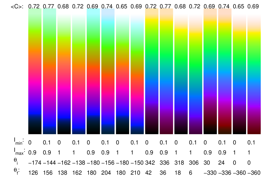
Figure 1: Color scales which maximize the average chroma $\langle C\rangle$, with the assumption of linear variation in hue and intensity, and 16 combinations of $I_{min}$ (0 or 0.1), $I_{max}$ (0.9 or 1), and $\theta_{f}-\theta_{i}$ (-360, -300, 300, or 360). For these 16 parameter sets, $\langle C\rangle$ is maximized over $\theta_{i}$.

Figure 1 gives the color scales that maximize the average chroma for the 16 combinations of parameters. The first eight start near cyan on the hue scale and move to blue, then magenta, red, yellow, green and cyan. The second eight move oppositely around the hue scale, and start at red, followed by magenta, blue, cyan, green, yellow, and red. The average chroma are the same in corresponding members of the two sets.

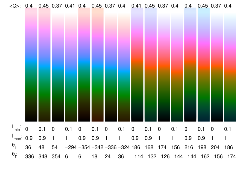
Figure 2: Color scales which minimize the average chroma over $\theta_{i}$, for the same parameters as in figure 1.

It is useful to know how much better the optimal color scales are in comparison to non-optimal scales. For a point of reference, in figure 2 we show the chroma-minimizing color scales at the same 16 parameters. These color scales are nearly (but not exactly) opposite in phase with respect to the chroma-maximizing scales in terms of hue. The first eight start near red, followed by yellow, green, cyan, blue, magenta, and red. The second eight start near cyan followed by green, yellow, red, magenta, blue, and cyan. The average chroma are 55-60% of those for the optimal scales at the same parameters. It is apparent that the colors in figure 2 are grayer than those in figure 1.

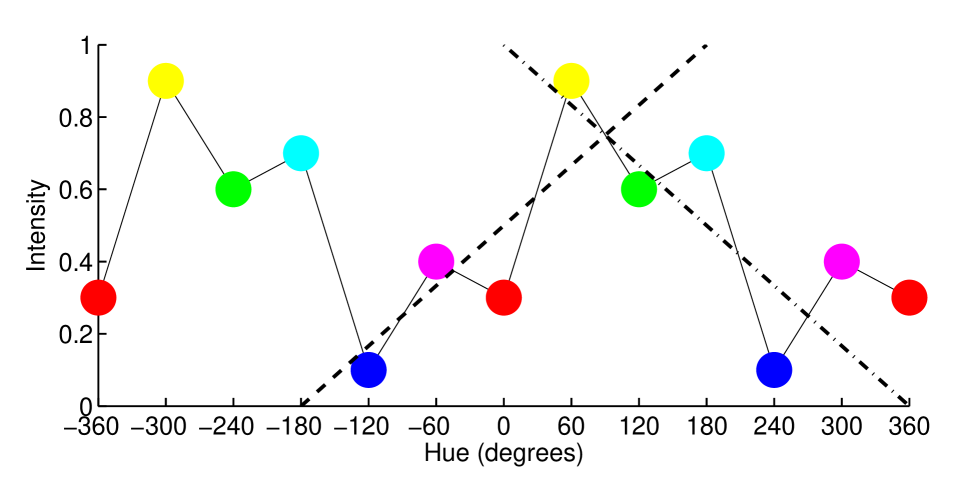
Figure 3: The chroma-maximizing scales with intensity plotted against hue, for $I_{min}=0$, $I_{max}=1$, and $\theta_{f}-\theta_{i}=$ 360 (dashed line) or -360 (dashed-dotted line). Also plotted are the intensities of the colors with chroma of 1 for each hue. These intensities linearly interpolate those of the six pure colors red, yellow, green, cyan, blue, and magenta.

One way of understanding these results is to plot the chroma-maximizing scales with their intensities versus their hues. We plot 2 of the 16 scales from figure 1 in this way in figure 3. At each hue, the intensity of the color with chroma equal to 1 is plotted as a piecewise linear black solid line which interpolates the six basic colors. The chroma-maximizing scales are plotted as dashed and dashed-dotted lines. Shifting these lines horizontally corresponds to changing $\theta_{i}$. With the $\theta_{i}$ shown (-180 and 360 degrees), the scales correlate most closely with the chroma-one colors. In both cases, blue occurs near the low-intensity end of the scale, and yellow near the high intensity end. Thus the scales incorporate the natural intensities of the pure colors.

References

- (1) K.N. Plataniotis and A.N. Venetsanopoulos. Color image processing and applications. Springer, 2000.
- (2) H.R. Kang. Computational color technology, volume 159. Society of Photo Optical Instrumentation Engineers, 2006.